1. Introduction
Reynolds-averaged Navier–Stokes (RANS) turbulence models such as the
 $k{-}{\it\epsilon}$
closure scheme (Launder & Spalding Reference Launder and Spalding1972) commonly use the turbulent-viscosity hypothesis (hereafter TVH) to simulate wall-bounded flows. In these models, the Reynolds stresses are linked with the mean shear rate (
 $S$
) through the turbulent (eddy) viscosity (
 ${\it\nu}_{t}$
). For a one-dimensional shear flow,
 ${\it\nu}_{t}$
is given by
 $$\begin{eqnarray}{\it\nu}_{t}=\frac{-\overline{u^{\prime }v^{\prime }}}{\text{d}\overline{U}/\text{d}y},\end{eqnarray}$$
where
 $\overline{U}$
is the mean streamwise velocity and
 $y$
is the vertical distance from the wall. Within the context of the TVH, dimensional reasoning can be used to recast
 ${\it\nu}_{t}$
in terms of characteristic scales of velocity
 $(U_{TVH})$
, length
 $(L_{TVH})$
and time
 $(T_{TVH})$
as
 $$\begin{eqnarray}{\it\nu}_{t}=U_{TVH}\cdot L_{TVH}=U_{TVH}^{2}\cdot T_{TVH}=L_{TVH}^{2}/T_{TVH}.\end{eqnarray}$$
Pope (Reference Pope2000) suggested that a favourable velocity scale for turbulent flows is
 $U_{TVH}=(-\overline{u^{\prime }v^{\prime }})^{1/2}$
, which consequently results in the characteristic length scale as
 $L_{TVH}=(-\overline{u^{\prime }v^{\prime }})^{1/2}/S$
and the characteristic time scale as
 $T_{TVH}=T_{S}=1/S$
. It should be noted that these derived scales are only the relevant scales of the flow within the framework of the TVH and should not be interpreted as the scales of turbulence.
In some turbulence closure schemes such as the standard
 $k{-}{\it\epsilon}$
model, which is the most commonly used two-equation closure scheme (Pope Reference Pope2000; Durbin & Pettersson Reif Reference Durbin and Pettersson Reif2011), the turbulent viscosity (
 ${\it\nu}_{t}$
) is derived by assuming local and approximate equilibrium between the production rate of the turbulent kinetic energy (
 $P$
) and the dissipation rate of the turbulent kinetic energy (
 ${\it\epsilon}$
) in a fully developed wall-bounded turbulent flow. This assumption implies that the transport terms that result due to the presence of the solid wall are negligible and hence simplifies analysis of the wall-bounded turbulence.
In addition to assuming equilibrium (i.e.
 $P\approx {\it\epsilon}$
), the turbulent viscosity of the
 $k{-}{\it\epsilon}$
model (
 ${\it\nu}_{t(k{-}{\it\epsilon})}$
) is developed by using the proposition of Kolmogorov (Reference Kolmogorov1942) to base the characteristic velocity scale on the turbulent kinetic energy
 $(k)$
such that
 $U_{TVH}=(-\overline{u^{\prime }v^{\prime }})^{1/2}=ck^{1/2}$
. Hence,
 ${\it\nu}_{t(k{-}{\it\epsilon})}$
is given by
 $$\begin{eqnarray}{\it\nu}_{t}\approx {\it\nu}_{t(k{-}{\it\epsilon})}=c^{4}\frac{k^{2}}{{\it\epsilon}}=C_{{\it\mu}}\frac{k^{2}}{{\it\epsilon}}.\end{eqnarray}$$
Here,
 $c$
is the square root of the stress-intensity ratio (i.e.
 $c=(|\overline{u^{\prime }v^{\prime }}|/k)^{1/2}$
) and is usually assumed to be constant in the log-law region. In the standard
 $k{-}{\it\epsilon}$
model,
 $c\approx 0.55$
or
 $c^{2}\approx 0.3$
is employed on the basis of empirical measurements, which implies that
 $C_{{\it\mu}}\approx 0.09$
.
For the
 $k{-}{\it\epsilon}$
model to work properly in the near-wall region, the turbulent (eddy) viscosity shown in (1.3) needs to be the same as the turbulent viscosity defined in (1.1). However, it is well known that this formulation (1.3) breaks down in the near-wall region of canonical wall-bounded flows and over-predicts the exact turbulent viscosity (
 ${\it\nu}_{t}$
). This failure is normally attributed to the fact that the stress-intensity ratio (
 $c^{2}$
) is not a constant in the near-wall region. Efforts to overcome this severe shortcoming have focused on modifications to the transport equations for
 $k$
and
 ${\it\epsilon}$
in conjunction with empirical damping functions to reduce
 ${\it\nu}_{t(k{-}{\it\epsilon})}$
in the near-wall region (see, e.g. Jones & Launder Reference Jones and Launder1973; Launder & Sharma Reference Launder and Sharma1974; Lam & Bremhorst Reference Lam and Bremhorst1981; Rodi & Mansour Reference Rodi and Mansour1993). These functions are not universal and tend to be ineffective when tested with different sets of DNS data.
Attempts have been made to model the near-wall turbulence without employing such damping functions. Durbin (Reference Durbin1991) proposed a model that solves for wall-bounded turbulence without recourse to a damping function. He argued that the wall-normal velocity fluctuation (
 $\overline{v^{\prime 2}}$
) is responsible for transport from the wall and not the total turbulent kinetic energy
 $(k)$
, as is assumed in the
 $k{-}{\it\epsilon}$
model. Hence, he developed a fourth-order turbulence closure scheme, namely the
 $k{-}{\it\epsilon}{-}\overline{v^{2}}$
model, where
 $\overline{v^{2}}$
represents
 $\overline{v^{\prime 2}}$
. Considering the model time scale as
 $T_{L}=k/{\it\epsilon}$
, the turbulent viscosity (
 ${\it\nu}_{t}$
) in Durbin’s model is computed as
 $$\begin{eqnarray}{\it\nu}_{t}=c_{{\it\mu}}^{\prime }\overline{v^{\prime 2}}\frac{k}{{\it\epsilon}},\end{eqnarray}$$
where
 $c_{{\it\mu}}^{\prime }$
is a constant taken as 0.20 by Durbin (Reference Durbin1991). Recently, Karimpour & Venayagamoorthy (Reference Karimpour and Venayagamoorthy2013) have shown that the
 ${\it\nu}_{t}$
formulation of Durbin’s model is insensitive to
 $c_{{\it\mu}}^{\prime }$
in the near-wall region. This is also in agreement with the experimental observations of Schultz & Flack (Reference Schultz and Flack2013), where they concluded that
 $-\overline{u^{\prime }v^{\prime }}$
and
 $\overline{v^{\prime 2}}$
are independent of the Reynolds number in the near-wall region. Durbin’s model has been extensively verified with both ‘a priori’ and ‘a posteriori’ tests, with remarkably good results.
In the current work, our main aim is to highlight the drawbacks of using the equilibrium assumption in conjunction with the use of the turbulent kinetic energy (
 $k$
) to infer the pertinent velocity scale in formulating a suitable turbulent viscosity. We also derive the appropriate scales within the framework of the TVH by analysing the turbulent viscosity formulation of Durbin (Reference Durbin1991). In § 2, a dimensional analysis of the turbulent viscosity formulation of the standard
 $k{-}{\it\epsilon}$
model (
 ${\it\nu}_{t(k{-}{\it\epsilon})}$
) is presented to derive the relevant scales inherent in this formulation and highlight the consequence of assuming equilibrium for inferring
 ${\it\nu}_{t(k{-}{\it\epsilon})}$
. The correlation of the turbulent kinetic energy (
 $k$
) with the anisotropic Reynolds stress (
 $\overline{u^{\prime }v^{\prime }}$
) is revisited in § 3, followed by a discussion on the appropriate scales for predicting near-wall turbulence. Finally, conclusions are given in § 4. In this study, different channel flow DNS datasets of Kim, Moin & Moser (Reference Kim, Moin and Moser1987) for
 $\mathit{Re}_{{\it\tau}}\approx 180$
, Moser, Kim & Mansour (Reference Moser, Kim and Mansour1999) for
 $\mathit{Re}_{{\it\tau}}\approx 395$
and 590, del Álamo et al. (Reference del Álamo, Jiménez, Zandonade and Moser2004) for
 $\mathit{Re}_{{\it\tau}}\approx 934$
and Hoyas & Jiménez (Reference Hoyas and Jiménez2006) for
 $\mathit{Re}_{{\it\tau}}\approx 2003$
are used together with the boundary layer experimental data of Marusic & Perry (Reference Marusic and Perry1995), for performing ‘a priori’ tests.
2. Assessment of the
 $k{-}{\it\epsilon}$
model turbulent viscosity

In this section, we derive the inherent scales in the turbulent viscosity formulation of the standard
 $k{-}{\it\epsilon}$
closure scheme and also discuss the possibility of introducing a universal
 $c$
. We use ‘a priori’ tests to reinforce our discussion.
2.1. Revisit of relevant characteristic scales and stress intensity
Using (1.3) and the proposition of Kolmogorov (Reference Kolmogorov1942) for the velocity scale (i.e.
 $U_{k{-}{\it\epsilon}}=ck^{1/2}$
), the relevant length scale inherent in
 ${\it\nu}_{t(k{-}{\it\epsilon})}$
can be derived as
 $$\begin{eqnarray}L_{k{-}{\it\epsilon}}=\frac{{\it\nu}_{t(k{-}{\it\epsilon})}}{U_{k{-}{\it\epsilon}}}=c^{4}\frac{k^{2}/{\it\epsilon}}{ck^{1/2}}=c^{3}\frac{k^{3/2}}{{\it\epsilon}}.\end{eqnarray}$$
Using
 $c=(-\overline{u^{\prime }v^{\prime }}/k)^{1/2}$
and
 $P=-\overline{u^{\prime }v^{\prime }}S$
, (2.1) can be rewritten as
 $$\begin{eqnarray}\displaystyle L_{k{-}{\it\epsilon}} & = & \displaystyle c^{3}\frac{k^{3/2}}{{\it\epsilon}}=\left(\frac{-\overline{u^{\prime }v^{\prime }}}{k}\right)^{3/2}\frac{k^{3/2}}{{\it\epsilon}}=\left(\frac{-\overline{u^{\prime }v^{\prime }}S}{{\it\epsilon}}\right)^{3/2}\left(\frac{{\it\epsilon}}{S^{3}}\right)^{1/2}\nonumber\\ \displaystyle & = & \displaystyle \left(\frac{P}{{\it\epsilon}}\right)^{3/2}\left(\frac{{\it\epsilon}}{S^{3}}\right)^{1/2}=\left(\frac{P}{{\it\epsilon}}\right)^{3/2}L_{c},\end{eqnarray}$$
where
 $L_{c}=({\it\epsilon}/S^{3})^{1/2}$
is the Corrsin scale, introduced for the first time by Corrsin (Reference Corrsin1958).
 $L_{c}$
shows the smallest eddy size that is deformed by the mean shear rate. The ratio
 $P/{\it\epsilon}$
can be expressed in terms of length scales as
 $$\begin{eqnarray}\frac{P}{{\it\epsilon}}=\frac{-\overline{u^{\prime }v^{\prime }}S}{{\it\epsilon}}=\frac{-\overline{u^{\prime }v^{\prime }}/S^{2}}{{\it\epsilon}/S^{3}}=\left(\frac{L_{TVH}}{L_{c}}\right)^{2}.\end{eqnarray}$$
Using (2.3), we can rewrite (2.1) as
 $$\begin{eqnarray}L_{k{-}{\it\epsilon}}=\left(\frac{P}{{\it\epsilon}}\right)^{3/2}\left(\frac{{\it\epsilon}}{S^{3}}\right)^{1/2}=\left(\frac{P}{{\it\epsilon}}\right)\frac{L_{TVH}}{L_{c}}\left(\frac{{\it\epsilon}}{S^{3}}\right)^{1/2}=\left(\frac{P}{{\it\epsilon}}\right)L_{TVH}.\end{eqnarray}$$
Equation (2.4) highlights the fact that while in the log-law region, where
 $P\approx {\it\epsilon}$
,
 $L_{k{-}{\it\epsilon}}$
is equal to
 $L_{TVH}$
and consequently
 $L_{c}$
, in the near-wall region both the length scale and therefore the turbulent viscosity
 $({\it\nu}_{t(k{-}{\it\epsilon})})$
are incorrect. Put another way, the turbulent viscosity from the standard
 $k{-}{\it\epsilon}$
model can be expressed in terms of the characteristic scales and the exact turbulent viscosity as
 $$\begin{eqnarray}{\it\nu}_{t(k{-}{\it\epsilon})}=c^{4}\frac{k^{2}}{{\it\epsilon}}=\left(ck^{1/2}\right)\left(c^{3}\frac{k^{3/2}}{{\it\epsilon}}\right)=\left(\frac{P}{{\it\epsilon}}\right)U_{TVH}L_{TVH}=\left(\frac{P}{{\it\epsilon}}\right){\it\nu}_{t}.\end{eqnarray}$$
Equation (2.5) clearly shows that in the near-wall region this formulation breaks down, as it is a function of
 $P/{\it\epsilon}$
. This implies that the failure of
 ${\it\nu}_{t(k{-}{\it\epsilon})}$
is independent of the fact that the exact value of
 $c$
is ambiguous and hence damping
 $c$
is not sufficient to make
 ${\it\nu}_{t(k{-}{\it\epsilon})}$
suitable for modelling the near-wall turbulence.
Furthermore, using
 $U_{k{-}{\it\epsilon}}=ck^{1/2}$
and
 $L_{k{-}{\it\epsilon}}$
the relevant time scale can be deduced as
 $$\begin{eqnarray}T_{k{-}{\it\epsilon}}=\frac{L_{k{-}{\it\epsilon}}}{U_{k{-}{\it\epsilon}}}=c^{2}\frac{k}{{\it\epsilon}},\end{eqnarray}$$
which can also be rewritten as
 $$\begin{eqnarray}T_{k{-}{\it\epsilon}}=c^{2}\frac{k}{{\it\epsilon}}=\frac{-\overline{u^{\prime }v^{\prime }}}{k}\frac{k}{{\it\epsilon}}=\left(\frac{-\overline{u^{\prime }v^{\prime }}S}{{\it\epsilon}}\right)\frac{1}{S}=\left(\frac{P}{{\it\epsilon}}\right)\frac{1}{S},\end{eqnarray}$$
which again shows that the time scale is only correct where equilibrium holds. This finding also shows that the traditionally assumed time scale
 $T_{L}=k/{\it\epsilon}$
in the standard
 $k{-}{\it\epsilon}$
model should be modified with
 $c^{2}$
.
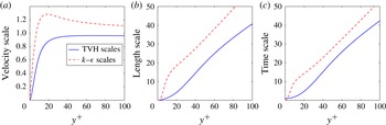
The comparisons of the standard
 $k{-}{\it\epsilon}$
model scales with the TVH scales are shown in figure 1, using
 $c\approx 0.55$
. It is obvious that (even in the log-law region) the standard
 $k{-}{\it\epsilon}$
model scales highly over-predict the corresponding characteristic scales, which raises the doubt about the suitability of assuming a constant
 $c\approx 0.55$
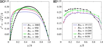
in the log-law region. To assess this issue further, figure 2 shows profiles of
 $c^{2}=-\overline{u^{\prime }v^{\prime }}/k$
obtained from direct numerical simulations (DNS) data of channel flows as well as high-Reynolds-number experimental boundary layer data. In figure 2,
 $\mathit{Re}_{{\it\tau}}=u_{{\it\tau}}h/{\it\nu}$
is the friction Reynolds number, where
 $h$
is half of the channel depth. Also,
 $\mathit{Re}_{{\it\theta}}=U_{e}{\it\theta}/{\it\nu}$
is the momentum thickness Reynolds number, with
 ${\it\theta}$
defined as the momentum thickness,
 $U_{e}$
as 99 % of the maximum velocity and
 ${\it\delta}$
as the boundary layer thickness. The profiles clearly show that assuming
 $c\approx 0.55$
or
 $c^{2}\approx 0.3$
is wrong. In fact, the profiles suggest that
 $c$
decreases with increasing Reynolds number in the log-law region, at least for this range of Reynolds numbers.
Comparison of (a)
 $U_{k{-}{\it\epsilon}}$
with
 $U_{TVH}$
; (b)
 $L_{k{-}{\it\epsilon}}$
with
 $L_{TVH}$
and (c)
 $T_{k{-}{\it\epsilon}}$
with
 $T_{TVH}$
; in a turbulent channel flow, computed from the DNS data of Hoyas & Jiménez (Reference Hoyas and Jiménez2006) for
 $\mathit{Re}_{{\it\tau}}=2003$
.

Comparison of
 $c^{2}=-\overline{u^{\prime }v^{\prime }}/k$
for different Reynolds numbers, using (a) DNS data of turbulent channel flows for
 $\mathit{Re}_{{\it\tau}}=2003,934,590,395$
and 180; and (b) experimental data of boundary layer flow of Marusic & Perry (Reference Marusic and Perry1995).

Now, we revisit the behaviour of
 $c$
. In a preliminary attempt, Karimpour & Venayagamoorthy (Reference Karimpour and Venayagamoorthy2013) have shown that by using the equilibrium assumption all the way to the wall, a turbulent viscosity formulation can be derived as
 ${\it\nu}_{t}\approx {\it\epsilon}/S^{2}$
, which implies that
 $c\approx 1/(ST_{L})^{1/2}$
. The comparison of their propositions with exact DNS computations showed small differences. However, it is clear that their formulation is not appropriate for modelling.
Here, we reassess the possibility of independently describing
 $c$
by relaxing the equilibrium assumption that Karimpour & Venayagamoorthy (Reference Karimpour and Venayagamoorthy2013) made. The square root of the stress-intensity ratio (
 $c=(-\overline{u^{\prime }v^{\prime }}/k)^{1/2}$
) can be recast as follows:
 $$\begin{eqnarray}c=\left(\frac{-\overline{u^{\prime }v^{\prime }}}{k}\right)^{1/2}=\left(\frac{-\overline{u^{\prime }v^{\prime }}S/{\it\epsilon}}{Sk/{\it\epsilon}}\right)^{1/2}=\left(\frac{P}{{\it\epsilon}}\right)^{1/2}\left(\frac{1}{ST_{L}}\right)^{1/2}=\frac{L_{TVH}}{L_{c}}\left(\frac{1}{ST_{L}}\right)^{1/2}.\end{eqnarray}$$
 $ST_{L}$
is the ratio of the turbulence (decay) time scale (
 $T_{L}$
) to the mean shear time scale (
 $1/S$
) and can be considered to be a measure of the linearization of the turbulent flow (Jiménez Reference Jiménez2013). Equation (2.8) clearly shows that
 $c$
and therefore the proposed velocity scale of Kolmogorov (Reference Kolmogorov1942) inherently depend on the behaviour of
 $P/{\it\epsilon}$
and hence
 $L_{TVH}$
. It can be inferred from figure 2 and (2.8) that
 $k$
cannot be an appropriate parameter of choice to describe
 $\overline{u^{\prime }v^{\prime }}$
. This highlights the reason for the lack of success in formulating a universal damping function to appropriately decrease
 $c$
in the near-wall region.
3. Correlation of the Reynolds stresses
In this section, we assess the correlation of the anisotropic Reynolds stress (
 $\overline{u^{\prime }v^{\prime }}$
) with isotropic Reynolds stresses. In his valuable work, Lumley (Reference Lumley1978) has discussed that the wall-normal velocity fluctuation (
 $\overline{v^{\prime 2}}$
) is a more appropriate velocity scale, since it mimics the behaviour of (
 $-\overline{u^{\prime }v^{\prime }}$
) better compared to
 $k$
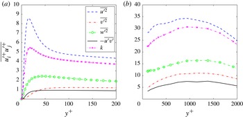
. Figure 3 confirms his assertion, and it can be seen that
 $k$
behaves similarly to the streamwise velocity fluctuation (
 $\overline{u^{\prime 2}}$
), while
 $\overline{v^{\prime 2}}$
closely matches
 $-\overline{u^{\prime }v^{\prime }}$
. As discussed in § 1, Durbin (Reference Durbin1991) made a similar argument and introduced the turbulent viscosity as
 ${\it\nu}_{t}=c_{{\it\mu}}^{\prime }\overline{v^{\prime 2}}(k/{\it\epsilon})$
.
Comparison of Reynolds stresses and the turbulent kinetic energy (
 $k$
) computed from (a) DNS data of Hoyas & Jiménez (Reference Hoyas and Jiménez2006) for
 $\mathit{Re}_{{\it\tau}}=2003$
; and (b) experimental boundary layer data of Marusic & Perry (Reference Marusic and Perry1995) for
 $\mathit{Re}_{{\it\theta}}=19\,133$
.

Durbin’s proposition for
 ${\it\nu}_{t}$
is widely used and its good comparison with exact
 ${\it\nu}_{t}$
is already shown in several works. Here, we test its efficacy for predicting
 $P/{\it\epsilon}$
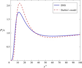
in the near-wall region. Figure 4 presents the comparison of
 $P/{\it\epsilon}$
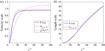
using Durbin’s formulation with the exact value from DNS data. While there is a slight mismatch, the comparison is still favourable and confirms the suitability of the turbulent viscosity formulation proposed by Durbin (Reference Durbin1991) for predicting the near-wall turbulence. This implies that the appropriate relevant scales in the context of the TVH are inherent in Durbin’s model. Therefore, it is instructive to derive the scales inherent in his model within the context of the TVH framework.
Comparison of Durbin’s model
 $P/{\it\epsilon}$
and the exact value computed from DNS data of Hoyas & Jiménez (Reference Hoyas and Jiménez2006) for
 $\mathit{Re}_{{\it\tau}}=2003$
.

Comparison of (a)
 $U_{k{-}{\it\epsilon}{-}v^{2}}$
and
 $(\overline{v^{\prime 2}})^{1/2}$
with
 $U_{TVH}$
; and (b)
 $L_{k{-}{\it\epsilon}{-}v^{2}}$
with
 $L_{TVH}$
computed from DNS data of Hoyas & Jiménez (Reference Hoyas and Jiménez2006) for
 $\mathit{Re}_{{\it\tau}}=2003$
.

Durbin (Reference Durbin1991) considered
 $T_{L}=k/{\it\epsilon}$
as the relevant time scale for his model with a lower bound set by a factor of the Kolmogorov time scale
 $({\it\nu}/{\it\epsilon})^{1/2}$
, where
 ${\it\nu}$
is the kinematic viscosity. However, as discussed earlier in this paper, the characteristic time scale in the context of the TVH is
 $T_{TVH}=T_{S}=1/S$
. Using
 $-\overline{u^{\prime }v^{\prime }}={\it\nu}_{t}S$
, the relevant velocity and length scales inherent in his model can be derived respectively, as follows:
 $$\begin{eqnarray}\displaystyle & \displaystyle U_{TVH}=\left(-\overline{u^{\prime }v^{\prime }}\right)^{1/2}\approx U_{k{-}{\it\epsilon}{-}v^{2}}={c^{\prime }}_{{\it\mu}}^{1/2}(ST_{L})^{1/2}\left(\overline{v^{\prime 2}}\right)^{1/2}, & \displaystyle\end{eqnarray}$$
 $$\begin{eqnarray}\displaystyle & \displaystyle L_{TVH}=\frac{\left(-\overline{u^{\prime }v^{\prime }}\right)^{1/2}}{S}\approx L_{k{-}{\it\epsilon}{-}v^{2}}=\left(\frac{{c^{\prime }}_{{\it\mu}}}{ST_{L}}\right)^{1/2}\left(\overline{v^{\prime 2}}\right)^{1/2}\frac{k}{{\it\epsilon}}. & \displaystyle\end{eqnarray}$$
 $L_{TVH}$
) and velocity (
 $U_{TVH}$
) are excellent, as shown in figure 5. Also, in figure 5(a),
 $(\overline{v^{\prime 2}})^{1/2}$
is shown for comparison. Moreover, it is clear that
 $T_{k{-}{\it\epsilon}{-}v^{2}}=L_{k{-}{\it\epsilon}{-}v^{2}}/U_{k{-}{\it\epsilon}{-}v^{2}}=1/S$
, which is equal to
 $T_{TVH}=1/S$
, and hence no comparison between the time scales is required. In figures 4 and 5,
 $c_{{\it\mu}}^{\prime }\approx 0.18$
is used, since it provides a better prediction of the overall turbulent viscosity across the channel depth for this set of DNS data.
In (3.1) and (3.2),
 $ST_{L}$
serves as an anisotropic correction to
 $\overline{v^{\prime 2}}$
(which can also be considered as a non-equilibrium correction in the near-wall region), while it is absent in the
 ${\it\nu}_{t}$
formulation given in (1.4). The reason for this is simply because
 $\overline{v^{\prime 2}}$
is less than
 $-\overline{u^{\prime }v^{\prime }}$
in the near-wall region (see figure 3), while
 $T_{L}=k/{\it\epsilon}$
is greater than
 $1/S$
in the near-wall region (see figure 1
c). These effects cancel out identically when computing the turbulent viscosity (i.e.
 ${\it\nu}_{t}=U_{k{-}{\it\epsilon}{-}v^{2}}\times L_{k{-}{\it\epsilon}{-}v^{2}}$
).
4. Concluding remarks
In this study, the validity of the equilibrium assumption in the near-wall region was revisited. Using dimensional reasoning, we have shown that the equilibrium assumption leads to incorrect prediction of the characteristic scales in the near-wall region and highlighted some of the shortcomings of using damping functions to model the near-wall turbulence. This was followed by a detailed discussion on the importance of introducing an appropriate velocity scale rather than the traditionally assumed scale
 $ck^{1/2}$
. To this end, the successful model of Durbin (Reference Durbin1991), which makes use of
 $\overline{v^{\prime 2}}$
instead of
 $k$
, was analysed and the relevant length and velocity scales were derived. Our analysis shows that inherently there is an anisotropic correction of
 $ST_{L}$
to Durbin’s model constant
 $(c_{{\it\mu}}^{\prime })$
that is not explicit in the original turbulent viscosity formulation in his model. ‘A priori’ comparisons of these relevant scales using DNS data are excellent and indicate their relevance in capturing the characteristic scales. Furthermore, the predicted behaviour of
 $P/{\it\epsilon}$
using Durbin’s turbulent viscosity formulation shows favourable comparison with the exact profile obtained from DNS data. Overall, this study highlights the fidelity of Durbin’s model in capturing the characteristic scales of turbulence (within the framework of the TVH) in the near-wall region.
Acknowledgements
The authors thank the three anonymous referees for their constructive comments and recommendations. We also wish to thank Professors I. Marusic, S. Hoyas, J. Jiménez and R. Moser for providing their detailed data for various wall-bounded flows. The support of the National Science Foundation under CAREER grant OCE-1151838 (Program Director: Dr E. Itsweire) is gratefully acknowledged. S.K.V. also gratefully acknowledges the support of the Office of Naval Research (Scientific officers: Dr T. Paluszkiewicz and Dr S. Harper).