1. Introduction
The ongoing COVID-19 pandemic (The Novel Coronavirus Pneumonia Emergency Response Epidemiology Team 2020) creates the need to measure and track mortality shocks in portfolios managed by actuaries. The intense nature of the first COVID-19 mortality shock in many countries means that traditional methods based around annual
 $q_x$
-style mortality rates are inadequate: mixing periods of shock and non-shock mortality will under-state the true intensity of a mortality spike. Furthermore, risk managers and decision-makers cannot wait until a full year’s experience becomes available, while administration functions need to plan staffing levels from week to week for processing surges in death notifications. Something akin to real-time mortality reporting is therefore needed, so continuous-time methodologies are strongly preferred.
There are two related practical issues. First, the short-term nature of the COVID-19 shock in some territories carries the risk of confounding with normal seasonal variation; see Rau (Reference Rau2007) for a comprehensive overview of human seasonal mortality and Richards et al. (Reference Richards, Ramonat, Vesper and Kleinow2020) for the specifics of seasonal mortality among pensioners and annuitants. Any assessment of the impact of COVID-19 on an insured portfolio must therefore take into account typical seasonal variation. Second, the most up-to-date available data will be affected by unreported deaths, so any methodology must handle the inherent delays in death reporting.
We present a simple, semi-parametric estimator that tracks portfolio mortality levels by operating on intervals defined by the gaps between dates of death. This means daily estimation of portfolio mortality levels where the data support it. We illustrate our approach by applying the estimator to annuitant portfolios in three countries, revealing the timing and impact of the first COVID-19 shock and comparing the size of the shock against past seasonal variation in those same portfolios. We further present a fully parametric model for delays in death reporting and show how this provides continuous forecasts of emerging portfolio mortality.
The plan of the rest of this paper is as follows: section 2 describes the data sets used in the paper, while section 3 defines and illustrates a semi-parametric estimator for the portfolio-level mortality hazard. Section 4 considers delays in reporting and recording of deaths. Section 5 presents a parametric model for such delays, and section 6 considers its effectiveness in terms of fit; section 7 examines the ability of the parametric OBNR (occurred but not reported) term to forecast unreported mortality, and how to use it to improve the semi-parametric estimator of section 3; section 8 concludes.
2. Data Description
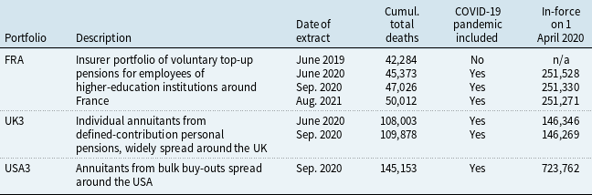
The data sets used in this paper comprise individual records from the insurer annuity portfolios described in Table 1. Due to the financial interest in not paying longer than necessary, administrators maintain accurate records of when annuities commence and when they cease. Such portfolios are like longitudinal studies with continuous recruitment: new benefit records are set up as people retire, but also when the death of the primary annuitant triggers an annuity to a surviving spouse.
Overview of portfolios and data extracts available. The naming convention is consistent with Richards et al. (Reference Richards, Ramonat, Vesper and Kleinow2020), as some of the same portfolios are used.

Direct extracts were made from the administration systems for the FRA and UK3 portfolios, as recommended by Macdonald et al. (Reference Macdonald, Richards and Currie2018, Section 2.2) to get the most up-to-date data. Extracts were taken at different times, and the corresponding cumulative death counts are shown in Table 1. The September 2020 extracts will be used for estimating the impact of the COVID-19 mortality shock in section 3, while earlier extracts for the same portfolio will be used for assessing delays in death reporting and recording in section 4.
Policy records were validated using the checks described in Macdonald et al. (Reference Macdonald, Richards and Currie2018, Sections 2.3 and 2.4). Insurer annuity portfolios often contain two or more policies per person, and so a data-preparation stage of deduplication is normally required for statistical modelling; see Macdonald et al. (Reference Macdonald, Richards and Currie2018, Section 2.5) for discussion of various approaches. The UK3 portfolio in particular contains many such duplicates. However, the FRA portfolio did not contain enough detail in two of the extracts to permit deduplication, so we will use the policy-level records without deduplication in this paper. This means that our mortality data are over-dispersed (Djeundje & Currie Reference Djeundje and Currie2011) due to some individuals receiving more than one annuity. As a result, the AICs in Tables 4 and 5 are somewhat over-stated, as they are computed using benefit records instead of lives.
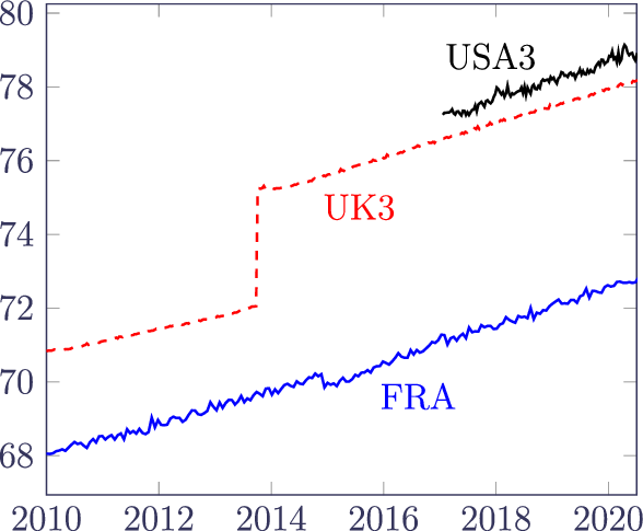
Figure 1 shows that the average age increased over the exposure period in all three portfolios, indicating that the numbers of new policies are not enough to stop the portfolios ageing. The large step increase in average age for UK3 is due to the transfer out of a block of annuities, while the small step decrease in average age for FRA is due to a batch of 9,572 new annuities in December 2014. We will therefore restrict our attention to experience data on or after 1 January 2015 to avoid step changes in the age composition of portfolios.
Average age over time of in-force annuitants in Table 1.

A key step in reinsurance transactions is the validation of the data available, and individual policy records enable particularly thorough data-quality checks (Macdonald et al., Reference Macdonald, Richards and Currie2018, Chapter 2). However, data-protection and privacy laws in many territories often restrict the sharing and processing of personal data; examples include GDPR in the EU and UK (Council of European Union 2016), CCPA in California (State of California Office of Legislative Counsel 2018) and PIPEDA in Canada (Minister of Justice for Canada 2018). Data-protection laws typically apply to personally identifiable data, i.e. data that could be used to identify a living person. However, Canadian laws are even stricter and further protect the personal data of the deceased for up to twenty years. Such laws tend to reduce the detail in data shared between counterparties for bulk annuities, longevity swaps and reinsurance treaties. This unfortunately also limits those counterparties’ ability to validate the experience data. Particularly problematic are cases where risk and therefore data are transferred between jurisdictions, e.g. from an insurer covered by the EU’s GDPR directive to a reinsurer outside the European Union. This forces the consideration of new techniques and tools for checking the validity of mortality-experience data (see Appendix 9).
A further issue for the accepting (re)insurer lies in deciding what data to discard due to the impact of reporting delays. Macdonald et al. (Reference Macdonald, Richards and Currie2018, p. 41) suggest discarding the six months of data prior to the extract date, but portfolios are likely to vary in the impact of national laws and administrative practices. A portfolio-specific measure of the impact of reporting delays would be better, which is considered in section 4. However, very few administration systems record data on reporting delays. An alternative is to compare closely spaced extracts, but this is less straightforward than it might seem, even for internal purposes. Many pension schemes and insurers outsource their administration, which can mean that data extracts have a cash cost. Also, when a reinsurance transaction is being considered, the ceding insurer will typically provide only a single extract of experience data. The same applies to pension schemes looking to transact a bulk annuity or longevity swap. A method of estimating reporting delays from a single data extract would therefore be useful, which is considered in section 5.
3. A Semi-parametric Estimator for Portfolio-Level Mortality
The mortality hazard,
 $\mu_{x,y}$
, is a function of age, x and calendar time, y, plus other risk factors such as gender, pension size and others; see Madrigal et al. (Reference Madrigal, Matthews, Patel, Gaches and Baxter2011) and Richards et al. (Reference Richards, Kaufhold and Rosenbusch2013) for examples. Various non-parametric estimators of mortality functions exist, but they typically only have one time-varying element (usually age). For example, the Nelson-Aalen estimator (Nelson, Reference Nelson1958) of the integrated mortality hazard and the Kaplan-Meier estimator of the survivor function (Kaplan & Meier Reference Kaplan and Meier1958) are usually defined with respect to age, leaving unmodelled heterogeneity with respect to calendar time. In this section, we consider non-parametric estimators defined with respect to calendar time, leaving age and other factors as unmodelled sources of heterogeneity. We note that such estimators will be in no sense useful for estimating the mortality of a portfolio for tasks like pricing and reserving. However, over short periods of time most portfolios do not change much in composition, and so such estimators might reveal insights into short-term variation in mortality levels.
Adapting the notation of Macdonald et al. (Reference Macdonald, Richards and Currie2018, p. 140), we consider a Nelson-Aalen estimator,
 $\hat\Lambda_{y,t}$
, of the cumulative hazard from calendar time y to
 $y+t$
. We turn dates into real numbers by taking the year and adding the number of days elapsed divided by the number of days in that year. For example, 2020 is a leap year, so the date 2020-03-14 is represented as 2020.199454 (=
 $2020+73/366$
). We create a set
 $\{y+t_i\}$
of
 $n_y$
distinct times (dates) of death. We define
 $d_{y+t_i}$
as the number of deaths occurring at time
 $y+t_i$
and define
 $l_{y+t_i^-}$
as the number of lives immediately before time
 $y+t_i$
. Our non-parametric estimator of the aggregate integrated hazard from time y to
 $y+t$
is shown in equation (1):
 \begin{equation} \hat\Lambda_{y,t} = \sum_{t_i\le t} \frac{d_{y+t_i}}{l_{y+t_i^-}}\end{equation}
An example of
 $\hat\Lambda_{y+t}$
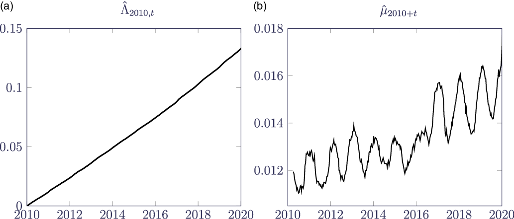
for the FRA portfolio is shown in Figure 2(a). The number of comparisons required for
 $\big\{l_{y+t_i^-}\big\}$
grows with the product of
 $n_y$
and the number of lives, so we use parallel processing over 63 threads to reduce calculation time (Butenhof Reference Butenhof1997).
(a) Nelson-Aalen estimate
 $\hat\Lambda_{2010,t}$
, (b) estimate
 $\hat\mu_{2010+t}$
with
 $c=0.5$
. Mortality is revealed to be a highly time-dependent process, with material swings based on the season. Source: own calculations using August 2021 extract of FRA portfolio described in Table 1.

We then use the Nelson-Aalen estimator in equation (1) to create a semi-parametric estimator of the mortality hazard in time,
 $\hat\mu_{y+t}$
, as per equation (2):
 \begin{equation} \hat\mu_{y+t} = \frac{1}{c}\left(\hat\Lambda_{y,t+c/2} - \hat\Lambda_{y,t-c/2}\right)\end{equation}
Equation (2) is a central difference around
 $\hat\Lambda_{y,t}$
with a bandwidth parameter of
 $c>0$
years. The result is shown in Figure 2(b) for the FRA portfolio. Equation (2) is essentially a uniform kernel estimator, and more sophisticated kernel estimators are available; see Anderson et al. (Reference Anderson, Borgan, Gill and Keiding1992), Section IV.2.1. In this paper, c is set subjectively, i.e. c is varied so that volatility is dampened enough to reveal underlying patterns. Larger values of c apply more smoothing, and setting
 $c>0.5$
will start to smooth out even seasonal variation. Equations (1) and (2) lend themselves to implementation in a spreadsheet or R, and thus for interactive setting of c. Appendix B contains R source for implementing equations (1) and (2) and plotting Figure 2.
Despite the major sources of unmodelled heterogeneity, the estimator in equation (2) is useful for revealing short-term fluctuations of mortality, as shown in Figure 2. Although
 $\hat\Lambda_{2010,t}$
appears linear to the naked eye,
 $\hat\mu_{2010+t}$
reveals the strong seasonality observed in many pensioner populations (Richards et al., Reference Richards, Ramonat, Vesper and Kleinow2020). The overall rising trend in Figure 2(b) is due to the increasing average age of the FRA portfolio shown in Figure 1, a reminder of why the semi-parametric approach is an exploratory tool and not a pricing tool. The amplitude of seasonal fluctuations increases with the increasing average age, a phenomenon measured in the FRA portfolio and others in Richards et al. (Reference Richards, Ramonat, Vesper and Kleinow2020, Section 5).
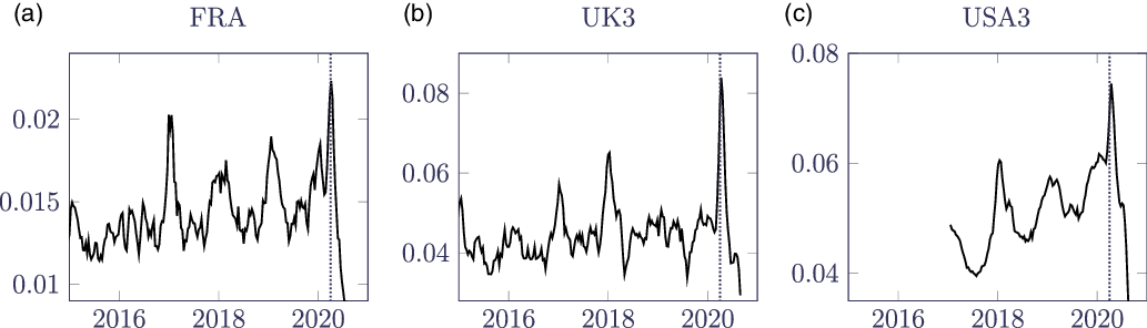
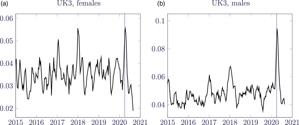
Equation (2) works best where there are several reported deaths per day. This applies to all three annuity portfolios in this paper, and even the modest-sized pension schemes in Appendix A have one or more deaths every day. However, term-assurance portfolios would have to be much larger, due to the younger average age and relative scarcity of deaths compared to annuity portfolios. Although the UK3 portfolio is the smallest in terms of policy counts (Table 1), its higher average age (see Figure 1) means there are more deaths per day than the much larger FRA portfolio. More deaths per day means that a portfolio can support a smaller value of c to reveal greater detail, as in Figure 3 where we can see the COVID-19 mortality spike in April 2020 for the FRA, UK3 and USA3 portfolios. The COVID-19 spike is lower for the FRA portfolio for three potential reasons: first, the portfolio has a lower average age (see Figure 1), and the mortality rate of those infected with SARS-CoV-2 increases strongly with age; see CCAES (2020) and Istat (2020); second, the portfolio is of highly educated individuals with a presumably higher socio-economic status and perhaps lower exposure risk (or better health behaviours); third, the FRA portfolio has longer delays in death notification (see section 4). Figure 3 also benchmarks the COVID-19 shocks against past seasonal variation: for the FRA portfolio, the COVID-19 spike is marginally higher than the winter period at the start of 2017, whereas for the UK3 portfolio the COVID-19 spike is at least a third higher than the 2017/2018 winter. For the UK3 portfolio, the death rate peaked at 19.6 per 100,000 annuities in the second week of January 2018, whereas it peaked at 26.8 in the first week of April 2020.
 $\hat\mu_{y+t}$
for September 2020 extracts of FRA, UK3 and USA3 portfolios with
 $c=0.1$
. 1 April 2020 is marked with a dotted vertical line. The vertical scales are different because of the younger average age of the FRA portfolio. y varies by portfolio, but only values of
 $y+t$
since 1 January 2015 are shown for comparability.

Figure 4 shows
 $\hat\mu_{2015+t}$
separately for males and females in the UK3 portfolio. The females in Figure 4(a) experienced a COVID-19 spike in April 2020 that is comparable to the spike in the winter of 2017/2018. In contrast, Figure 4(b) shows that males experienced far worse COVID-19 mortality, with a peak death rate of 29.8 per 100,000 in the first week of April 2020 against a prior peak death rate of 23.8 per 100,000 in the first week of January 2018. The heavier COVID-19 mortality of males was also present in the data of CCAES (2020) and Istat (2020).
 $\hat\mu_{2015+t}$
with
 $c=0.1$
separately for males and females in UK3 portfolio. 1 April 2020 is marked with a dotted vertical line. The vertical scales are different because males have a higher mortality rate than females.

The contrast between Figures 3(b) and 4(a) and (b) shows a drawback of the semi-parametric method: stratifying the UK3 data set by gender leads to a weaker signal and thus greater noise for a given value of c, or else the need for a higher value of c to compensate for the extra volatility.
Equation (2) is useful for exploratory analysis, and graphs like Figure 3 are useful for communication with non-experts. One practical aspect of equation (1) is that only three data items for each annuity are required for its computation: (i) the annuity commencement date, (ii) the date of cessation of observation (death, early withdrawal or the extract date) and (iii) whether the cessation is a death. This means that no personal data are required for the calculation of equation (2). This is a useful feature when modern data-protection and privacy laws restrict both the use and sharing of personally identifiable information (PII); indeed, the data for USA3 could only be shared for this research precisely because they contained no PII. Data privacy and further applications of the semi-parametric approach are discussed in Appendix A.
However, there are some drawbacks of equation (2). One is that
 $\hat\mu_{y+t}$
is not defined for the last
 $c/2$
years of the experience data. For smaller portfolios requiring larger values of c (see Figure A.2), this reduces the usefulness of the semi-parametric estimator as a timely statement of recent mortality. Furthermore, even where
 $\hat\mu_{y+t}$
is defined, the most recently calculated values are affected by unreported deaths – the FRA and USA3 portfolios in Figure 3 show particularly pronounced drops in reported mortality levels in mid-2020 caused by such delays. We therefore need a methodology that can produce results that are both up-to-date and adjust for reporting delays. Before this, however, we first explore the nature and extent of late-reported deaths in the FRA and UK3 portfolios, as these portfolios have more than one data extract.
4. Reporting Delays (OBNR)
Figures 3(a) and (c) show a dramatic fall in apparent mortality after the peak in April 2020, far below the level of pre-pandemic mortality. This is due to delays in the reporting and recording of deaths, i.e. occurred but not reported (OBNR) to use the terminology of Lawless (Reference Lawless1994). Such OBNR effects make the estimator in equation (2) less useful for the period leading up to the extract date. This is in addition to the loss of the
 $c/2$
years prior to the extract date due to the nature of equation (2). This gives rise to a trio of practical questions: (i) how extensive is the OBNR effect, (ii) how far back does the OBNR effect matter, and (iii) can we adjust for OBNR to compensate?
We assume that a death takes a time
 $v>0$
to be notified to the insurer. v is referred to as secondary data, i.e. information about the death reporting rather than about the underlying life. For the FRA and UK3 data sets, we each have two separate extracts at times
 $u_1$
and
 $u_2$
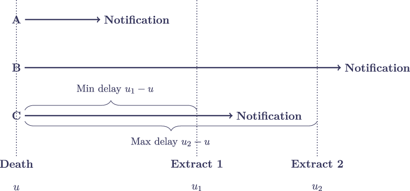
in 2020. Figure 5 shows the three different ways in which a death at time
 $u<u_1$
can be related to the two extracts. Type A deaths both occur and are reported before
 $u_1$
. Without separate recording of the notification date, such deaths tell us only that
 $v\in(0, u_1-u]$
. Type B deaths occur before
 $u_1$
but are still unreported by
 $u_2$
. Such deaths are unknown to us, and so our delay data are right-truncated. Type C deaths occur before
 $u_1$
, but are only reported between
 $u_1$
and
 $u_2$
; here the delay data are interval-censored (Collett Reference Collett2003, Chapter 9) and all we can say about the reporting delay is that
 $v\in(u_1-u, u_2-u]$
.
Three deaths A, B, and C occurring on the same date, u, and how their notification relates to data extracts at times
 $u_1$
and
 $u_2$
(
 $u<u_1<u_2$
).

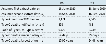
We do not know the exact date of each extract, so we assume it is the day after the last date of death. This simplifying assumption has a significant impact on the AICs in the likes of Tables 4 and 5, although it does not change the conclusion that the OBNR effect is statistically significant. Table 2 shows summary details of the late-reported deaths observed between two successive extracts of the FRA and UK3 portfolios.
Summary of observed reporting delays between successive extracts.

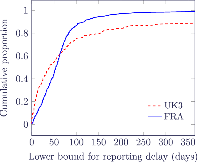
Table 2 shows that the FRA portfolio has a bigger OBNR issue than the UK3 portfolio, as the ratio of Type C deaths to Type A deaths in 2020 is much higher. We also see that both portfolios have occasional delays lasting more than a decade. Figure 6 shows the ogives of the minimum reporting delays for Type C deaths, i.e.
 $u_1-u$
. Although Figure 6 makes it appear that the UK3 portfolio has a worse reporting delay due to the lower cumulative proportion, Table 2 shows that this is actually because the Type C deaths for UK3 are the most seriously delayed cases.
Ogives of lower bound for Type C reporting delays in days. The horizontal axis is restricted, as the presence of decade-long delays otherwise distorts the plot.

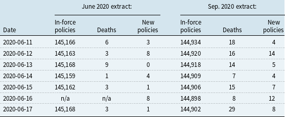
To illustrate the impact of OBNR deaths, Table 3 shows a week in June 2020 for the UK3 portfolio. As noted in Dodd et al. (Reference Dodd, Streftaris, Waters and Stott2015, p. 108), there are numerous effects of OBNR deaths on the likes of equation (2). There are three direct ways for missing deaths to have an impact: (i) there are more distinct death times than the
 $n_y$
ones observed in a given extract, as demonstrated by the row for 16 June 2020, (ii) the
 $d_{y+t_i}$
death counts are higher, and (iii)
 $l_{y+t_i}^-$
counts are lower due to other late-reported deaths for the period before 11 June 2020. This effect stretches back months prior to the extract, as can be seen in the in-force policy counts at 1 April 2020 in Table 1. Points (ii) and (iii) both act on equation (2) to progressively under-state the mortality hazard closer to the extract date.
Impact of late-reported deaths comparing two extracts of UK3 portfolio in Table 1. The later extract not only contains more deaths due to reporting delays, but reduced in-force counts as well. In the June 2020 extract, there were no deaths on 16 June and so no policy count was calculated for that date.

For portfolios like UK3, there is an indirect fourth impact on policy counts from late-reported deaths: upon the death of a primary annuitant, a surviving spouse’s annuity may be set up. In addition to past death counts increasing due to reporting delays, policy counts may also increase if a back-dated spouse’s annuity is set up. Such a case would lead to
 $d_{y+t_i}$
increasing by 1 at the time of death of the primary annuitant, but the corresponding
 $l_{y+t_i^-}$
count would be unchanged due to the new spouse’s annuity offsetting the main annuitant’s death. The columns of new policy counts in Table 3 illustrate the impact of retrospective spouse annuities being set up.
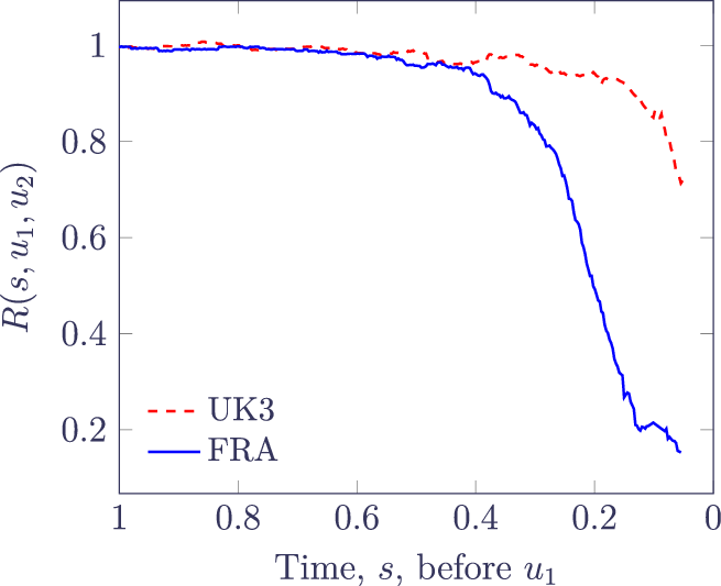
The impact of OBNR can be expressed as a function,
 $R(s, u_1, u_2)$
, of the time
 $s>0$
prior to the extract at
 $u_1$
.
 $R(s, u_1, u_2)$
is the ratio of the
 $\hat\mu_y$
estimates using extracts at times
 $u_1$
and
 $u_2$
, as in equation (3):
 \begin{equation} R(s, u_1, u_2) = \frac{\hat\mu_{u_1-s} {\rm\ using\ extract\ at\ time\ } u_1}{\hat\mu_{u_1-s} {\rm\ using\ extract\ at\ time\ } u_2} \end{equation}
R is only defined for
 $s>c/2$
and is plotted in Figure 7 for the FRA and UK3 portfolios. Both portfolios happen to have extracts for June 2020 (
 $u_1$
) and September 2020 (
 $u_2$
), and there is a steady fall in reported mortality in the months leading up to the June 2020 extract in each case (dramatically so for the FRA portfolio).
 $R(s, u_1, u_2)$
for FRA and UK3 portfolios. The horizontal axis is reversed.

Figure 7 shows that OBNR most affects the recent mortality estimates. Indeed, the most recent FRA ratio in Figure 7(a) is probably unreliable due to very small numbers of deaths. This is partly due to different insurer administration processes, but also to national differences in death registration and probate handling. In the UK, for example, insurers can use monthly feeds of deaths from the General Registrar’s Office to match possible deaths among their annuitants instead of waiting for notification.
The semi-parametric estimates of OBNR in Figure 7 are not wholly smooth, and they are undefined for the period
 $c/2$
years prior to the extract at time
 $u_1$
. R is also dependent on the second extract at time
 $u_2$
picking up all the late-reported deaths, which is at best an approximation due to Type B deaths – Table 2 shows that decade-long delays can occur.
A better approach would be a parametric model, especially one that operated on a single data extract, since there are many scenarios where only one extract is available; examples include reinsurance pricing, bulk annuities and longevity swaps, where the ceding pension scheme or insurer only makes available a single data extract. However, even actuaries working within an insurer can sometimes find it difficult to get closely spaced extracts, particularly if administration is outsourced to a third party.
5. A Parametric Model for Reporting Delays
We first note that we are interested in reporting delays only (OBNR), rather the combined delay-and-cost insurance models (IBNR) of Haastrup & Arjas (Reference Haastrup and Arjas1996) and Dodd et al. (Reference Dodd, Streftaris, Waters and Stott2015). Such IBNR models are “cost-orientated, discrete-time models” (Jewell Reference Jewell1989), whereas we require a pure delay model operating in continuous time.
There are numerous delay-only models, including for AIDS surveillance (Lawless Reference Lawless1994), HIV incubation time (Kalbfleisch & Lawless), cancer diagnosis and reporting to a central registry (Midthune et al., Reference Midthune, Fay, Clegg and Feuer2005) and even delays in detecting bugs in software (Jewell Reference Jewell1985). A common theme in these models is the availability of secondary data, specifically the date of notification of death in addition to the date of death itself. Delay data are necessarily right-truncated (Midthune et al., Reference Midthune, Fay, Clegg and Feuer2005), and in some cases, missing dates of notification can be accurately determined retrospectively (Kalbfleisch & Lawless). However, in the examples of the FRA and UK3 portfolios our delay data are additionally interval-censored (Collett Reference Collett2003, Chapter 9) as well as right-truncated.
Jewell (Reference Jewell1989) presents four classifications based on the availability of secondary data on delays and concludes that categories with missing dates of notification are “uninformative and useless” with respect to Bayesian methods. However, interval-censored delays are not entirely missing and are therefore neither uninformative nor useless, as shown in the distribution of lower bounds for reporting delays in Figure 6. Nevertheless, inference using interval-censored, right-truncated data is tricky, and for many insurers taking two extracts might not be practical. We therefore seek an approach that can infer OBNR from a single data extract.
We model OBNR-affected observed mortality,
 $\mu_{x,y}^{OBNR}(u_j)$
, which is related to actual mortality,
 $\mu_{x,y}^{*}$
, as in equation (4):
 \begin{equation} \mu_{x,y}^{OBNR}(u_j) = \mu_{x,y}^{*}\rho(u_j-y, \lambda_1) \end{equation}
where
 $\rho(s, \lambda_1)$
is an OBNR scaling factor reflecting the fact that not all mortality is reported in a timely manner. s is the positive-valued time before the date of extract,
 $u_j$
, and
 $\lambda_1$
is the decay parameter reflecting how quickly the OBNR effect changes with s.
 $\rho(s, \lambda_1)$
implicitly allows for unreported deaths of both Type B and Type C in Figure 5 by modelling the shortfall in mortality as y approaches the extract date,
 $u_j$
(see for example the shortfall demonstrated by the large negative residuals in Figure 10(a)). In most ordinary business circumstances, there will just be a single extract (
 $j=1$
), but we use the index j to allow for the circumstances where a second extract is available, as for the FRA and UK3 portfolios. We note an important difference between equation (4) on one hand and existing IBNR models and pure delay models on the other: the OBNR in our data is a nuisance effect and we only want to eliminate it. Both the function
 $\rho$
and the parameter
 $\lambda_1$
are therefore used in estimation, but neither plays any role in applications of the parameterised model
 $\mu^{*}_{x,y}$
, such as pricing or reserving. The approach in equation (4) assumes that mortality reporting at any age is presumed delayed by a function of time before the extract, whereas Black et al. (Reference Black, Hsu, Sanders, Schofield and Taylor2017), pp. 2016–2017 assume that some deaths at advanced ages are never reported (and never will be).
 \begin{equation} {\rm Logistic} \;:\; se^{\lambda_1}/(1+se^{\lambda_1}) \end{equation}
 \begin{equation} {\rm Exponential} \;:\; 1-\exp(-se^{\lambda_1})\end{equation}
 \begin{equation} {\rm Inverse\ tangent} \;:\; \frac{2}{\pi}\tan^{-1}(se^{\lambda_1})\end{equation}
 \begin{equation} {\rm Gaussian} \;:\; 2\Phi\left(se^{\lambda_1}\right)-1\end{equation}
 \begin{equation} {\rm Inverse\ exponential} \;:\; 2\left(1+\exp\left(-se^{\lambda_1}\right)\right)^{-1}-1\end{equation}
 \begin{equation} {\rm Squared\ exponential} \;:\; 1-\exp(\!-s^2e^{\lambda_1}) \end{equation}
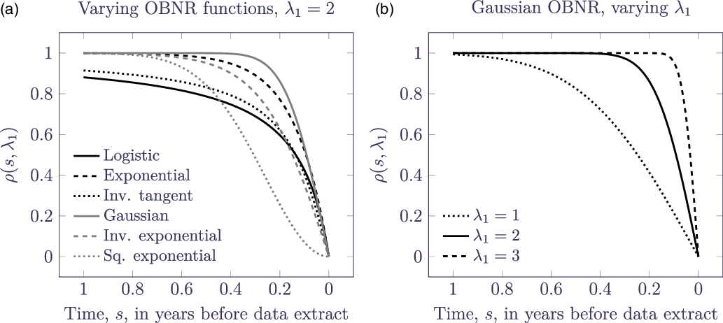
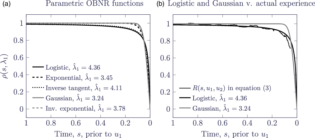
Some candidate single-parameter functions for
 $\rho$
are listed in equations (5)–(10) and plotted in Figure 8 for a specimen value of
 $\lambda_1$
; alternative functions with two or more parameters would be possible, although we arguably achieve an approximation of two-parameter flexibility by having a wide choice of single-parameter functions. Figure 8(a) shows the variety of shapes possible, allowing the choice of function and parameter
 $\lambda_1$
to fit the delay shape of a given portfolio. Figure 8(b) shows the role of the decay parameter,
 $\lambda_1$
, with lower values meaning more OBNR.
(a) OBNR functions with
 $\lambda_1=2$
, (b) Gaussian OBNR function with varying
 $\lambda_1$
. The horizontal axis is reversed for comparison with Figure 7.

One aspect of equation (4) is vulnerability to confounding (Midthune et al., Reference Midthune, Fay, Clegg and Feuer2005, p. 69). The choice of a function that is close to 1 until near the extract date forces the parameter
 $\lambda_1$
to pick up mostly OBNR effects. However, confounding of OBNR effects with seasonal effects could happen when
 $s<0.5$
, say because
 $u_j$
was in the summer and so mortality would be falling from the winter peak (Richards et al., Reference Richards, Ramonat, Vesper and Kleinow2020); equally, if
 $u_j$
were in the winter, the rising mortality since the summer would lead to under-stated OBNR effects. For
 $s\gg 0.5,$
there is also the risk of confounding OBNR effects with a time trend (Midthune et al., Reference Midthune, Fay, Clegg and Feuer2005, p. 62). To reduce the impact of confounding, any model attempting to allow for OBNR effects should therefore include both a time trend and a seasonal component, albeit strong correlations may remain between estimates (see Table B.3 in Appendix B). To address the seasonal aspect of mortality, we use the cosine model from Richards et al. (Reference Richards, Ramonat, Vesper and Kleinow2020, Section 8), as shown in equation (11):
 \begin{equation} \log\mu^*_{x,y} = \log \mu_{x,y}+e^\zeta\cos\left(2\pi(y-\tau)\right)\end{equation}
where
 $\tau\in [0,1)$
represents the proportion of the year after January
 $1^{\rm }$
when mortality peaks and
 $e^\zeta$
is the peak additional mortality at that time (on a logarithmic scale). The two-parameter model for seasonal mortality in equation (11) simultaneously identifies (i) the amplitude of the average-to-peak seasonal variation (
 $e^\zeta$
) and (ii) the point after January 1st corresponding to the winter mortality peak (
 $\tau$
). The full trough-to-peak variation is
 $2e^\zeta$
, and the definition of equation (11) forces
 $\tau$
to identify the winter peak, as opposed to the summer trough; we also assume that the peak is coincident in each of the years covered by a particular data set.
 $\mu_{x,y}$
is the non-seasonal component to the mortality hazard. The specific form of
 $\mu_{x,y}$
will depend on the age range under study,
 $x\in [x_0, x_1]$
say. Here we will use a variant of the Hermite II model of Richards (Reference Richards2020), as shown in equation (12):
 \begin{equation} \log\mu_{x,y} = (\alpha + \delta(y-2000))h_{00}(t) + m_0 h_{10}(t) + \omega h_{01}(t)\end{equation}
where
 $t=(x-x_0)/(x_1-x_0)$
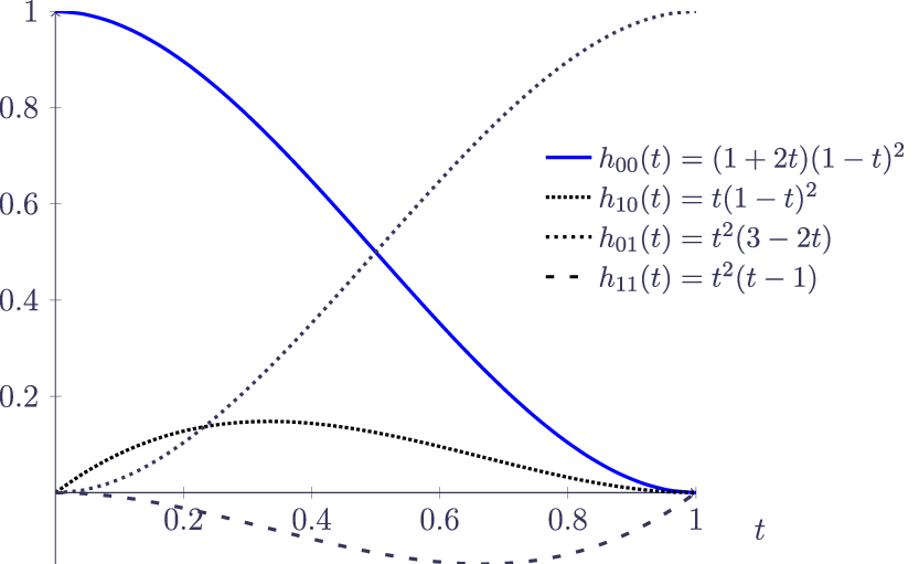
and the h functions are the cubic Hermite polynomials (Kreyszig Reference Kreyszig1999, p. 868) shown in Figure 9.
 $\delta$
is a time-trend parameter that allows mortality levels to rise or fall evenly over the exposure period; the modulation of
 $\delta$
by multiplying with
 $h_{00}(t)$
reduces the impact with age and means that mortality levels can change at younger ages, but are largely invariant at the oldest ages.
Hermite basis splines for
 $t\in[0, 1]$
.

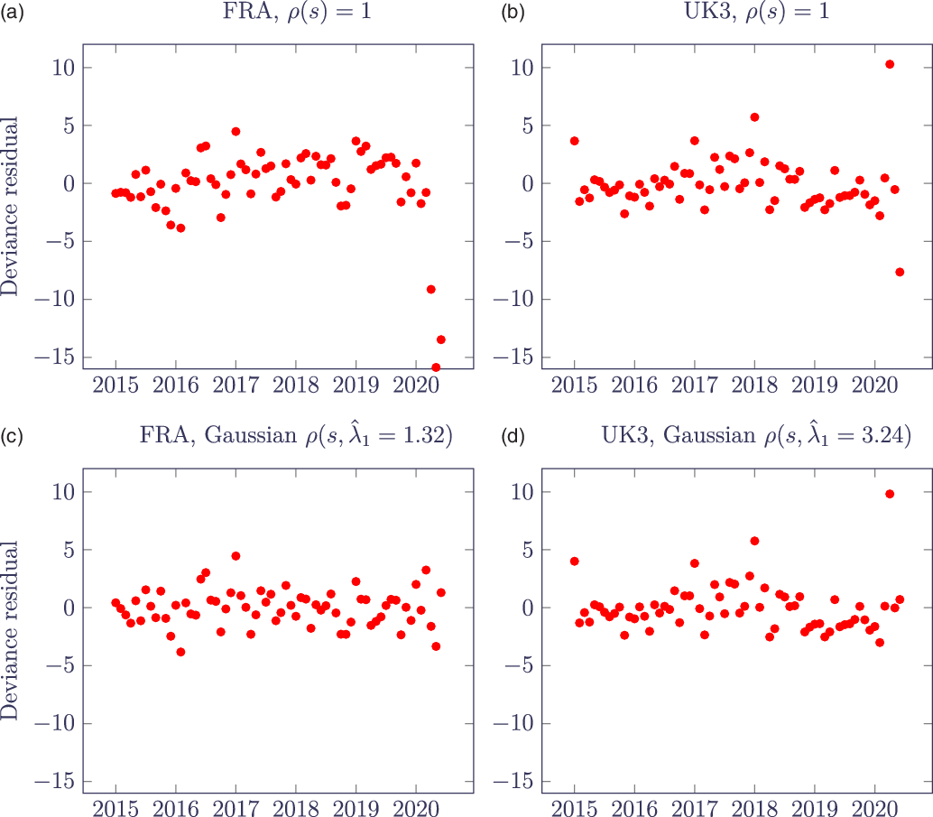
Monthly deviance residuals from model fits to June 2020 data for FRA and UK3 portfolio with and without a Gaussian OBNR term.

To fit a survival model to individual data, we maximise the log-likelihood function in equation (13) (Macdonald et al., Reference Macdonald, Richards and Currie2018, Section 5.3) for the OBNR-affected mortality hazard,
 $\mu_{x,y}^{OBNR}(u_j)$
, at age x at calendar time y using an extract at time
 $u_j$
. Each life i enters observation at age
 $x_i$
at calendar time
 $y_i$
and is observed for
 $t_i$
years.
 $d_i$
is an indicator variable taking the value 1 if life i is reported to have died at age
 $x_i+t_i$
, or 0 otherwise. The potential for bias due to OBNR lies in the fact that cases with
 $d_i=1$
are by definition unaffected by reporting delays, while cases with
 $d_i=0$
may be affected.
 $H_{x,y}(t;\;u_j)$
is the integrated hazard function in equation (14). We refer to Richards et al. (Reference Richards, Ramonat, Vesper and Kleinow2020, Appendix A) for implementation details of numerical integration of seasonally fluctuating hazard functions.
 \begin{equation} \ell = -\sum_{i\,=\,1}^n H_{x_i,y_i}(t_i;\;u_j) + \sum_{i\,=\,1}^n d_i \log\mu_{x_i,y_i}^{OBNR}(u_j)\end{equation}
 \begin{equation} H_{x,y}(t;\;u_j) = \int_0^t \mu_{x+s,y+s}^{OBNR}(u_j)ds\end{equation}
Equation (13) is the log-likelihood for a survival model with left-truncated data; see Macdonald et al. (Reference Macdonald, Richards and Currie2018, Section 4.3). This contrasts with survival models used in medical research, where left-truncation is rare and where likelihoods are usually for non-left-truncated data (Collett Reference Collett2003, Chapter 6). Note also that the structure of equation (4) means that OBNR effects are allowed for without having to deal with the interval-sensored, right-truncated nature of reported delays, i.e. we do not need any secondary data on delays.
6. Effectiveness of the Parametric OBNR Model
In this section, we look at the effectiveness of the parametric OBNR model in terms of model fit. Figure 10 shows the deviance residuals (McCullagh & Nelder, Reference McCullagh and Nelder1989, p. 39) without an OBNR term (upper panels,
 $\rho(s)=1$
) and with a Gaussian OBNR term (lower panels). Both portfolios have large negative residuals due to OBNR leading up to the extract date in June 2020, although Figure 10(a) shows that the FRA portfolio has a more severe OBNR effect with very large negative residuals.
Figure 10(d) shows that the UK3 portfolio has been affected more strongly by COVID-19 mortality, with a residual of +10 for the fourth month of 2020 (+10.3 without the OBNR term and +9.8 with it). The three next largest positive residuals in Figure 10(d) are all for January, reflecting (i) the excess winter mortality beyond the simple cosine model of equation (11) and (ii) that the COVID-19 mortality is worse than the worst recent winter excess. The lower value of
 $\hat\lambda_1$
for FRA indicates a slower OBNR decay rate, and thus a larger OBNR effect.
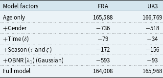
Table 4 shows the stepwise development of the AIC (Akaike Reference Akaike1987), dispensing with the small-sample correction as the number of lives is very large (Macdonald et al., Reference Macdonald, Richards and Currie2018, p. 98). For both portfolios, the inclusion of a time trend makes the smallest improvement in model fit, while the larger change in fit due to the OBNR effect in the FRA portfolio reflects the stark change between panels (a) and (c) in Figure 10. The OBNR functions in equations (5)–(10) do not allow for a (quite reasonable) link between reporting delays and age. However, they do allow for interactions between
 $\lambda_1$
and categorical factors, and we find that neither the FRA nor the UK3 portfolio has significant variation in OBNR by gender.
Development of AIC for models fitted stepwise to experience data spanning 1st Jan. 2015 to June 2020.

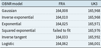
Table 5 shows the differences in fit for the various OBNR models in equations (5)–(10). Although these two portfolios differ in the extent and timing of their OBNR, the various OBNR functions have a similar order with respect to the AIC, with the Gaussian OBNR model providing the best (or best-equal) fit. The exception is the squared-exponential OBNR model, which failed to fit properly as the seasonal component of the model would not fit. Refitting the model with
 $m_0=0$
in equation (12) however worked, suggesting an occasionally problematic interplay between parameters.
AICs for OBNR models fitted to experience data spanning 1st January 2015 to June 2020.

7. “Nowcasting” Unreported Deaths
In this section, we look at the ability of a parametric OBNR model fitted to a single data extract to predict unreported deaths. We borrow the term “nowcasting” from economics (Bańbura et al. Reference BaŃbura, Giannone, Modugno, Reichlin, Elliott and Timmermann2013), as economists often also find themselves in the analogous position of predicting the current and recent state of a variable (such as GDP) that is typically only known after a time lag. We will fit the model for the OBNR-affected mortality of section 5 to the data for the June extract, and then we compare these OBNR functions to the effect of pre-June deaths reported by September. For the actual delay effect, we will use the semi-parametric R function of equation (7); this will not be a complete statement of OBNR due to still-unreported Type B deaths, but it will be a useful comparison.
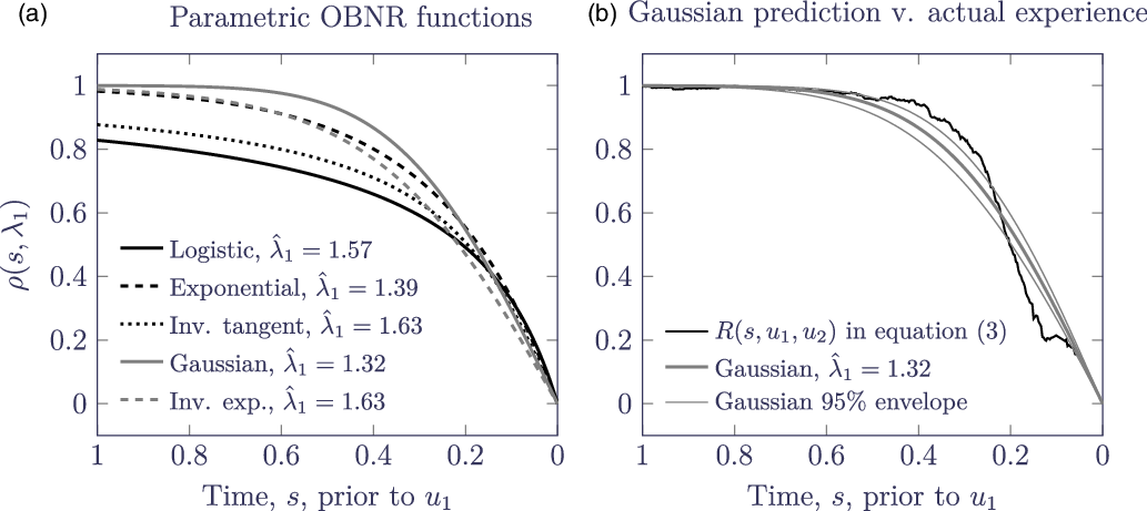
Figure 11(a) shows the fitted OBNR curves,
 $\rho(s, \lambda_1)$
, for the FRA portfolio, while Figure 11(b) shows the best-fitting Gaussian OBNR curve versus the semi-parametric
 $R(s, u_1, u_2)$
from Figure 7(a). Figure 11(b) shows that it is possible to make workable estimates of mortality OBNR for a portfolio based on just a single extract of data, i.e. without any secondary data on the delays themselves – the fitted OBNR adjustment based on data up to time
 $u_1$
follows the broad shape and trajectory of the OBNR in the subsequent experience after
 $u_1$
. In this sense, the OBNR function is actually a short-term forecast based on patterns leading up to the extract date.
(a) Estimated OBNR functions for June 2020 extract for FRA portfolio, (b) comparison of June OBNR estimates with OBNR function with lowest AIC against subsequent estimated OBNR using September 2020 extract. Panel (b) shows that the best-fitting parametric OBNR function using the June extract proved to be a workable overall forecast of the OBNR; this is despite the fact that the precise trajectory of the actual OBNR lies outside the 95% confidence envelope for the estimated OBNR function. The horizontal axes are reversed.

(a) Estimated OBNR functions for June 2020 extract for UK3 portfolio, (b) comparison of OBNR estimates with highest and lowest AICs against subsequent estimated OBNR using September 2020 extract. The OBNR functions with the joint-equal lowest AIC in the June extract proved to be poor projections of what the estimated OBNR was using the September extract; in fact, the OBNR functions with the highest AIC (logistic and inverse tangent) would have been better forecasts. The horizontal axes are reversed.

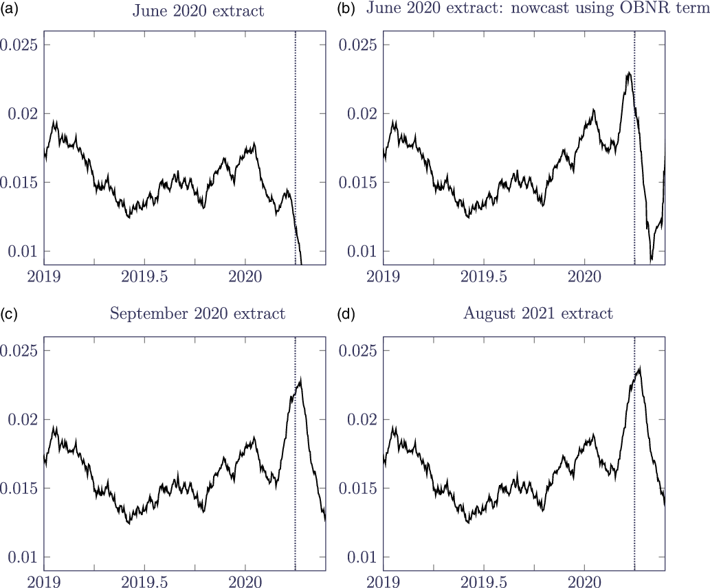
 $\hat\mu_{2019+t}$
for FRA portfolio with
 $c=0.1$
: (a) calculated using June 2020 extract; (b) nowcast using Gaussian OBNR function estimated from June 2020 extract; (c) calculated using September 2020 extract; (d) calculated using August 2021 extract. The vertical dotted line in each panel is at 1st April 2020.

In contrast, Figure 12(b) shows that for the UK3 portfolio the best-fitting of the OBNR functions in June proved to be a poorer forecast of the actual experience represented by the semi-parametric estimate using the late-reported deaths to September. In fact, the two poorest-fitting OBNR functions would have done a better job. This contrast can perhaps be explained by the fact that the UK3 portfolio has a much smaller OBNR issue, as shown in Figure 7. A possible reason for the better performance of the parametric OBNR function for the FRA portfolio is that the OBNR issue is both larger and affects a longer period of time leading up to the extract. This is suggested by the pattern of residuals in Figure 11(a). The parametric OBNR functions therefore work best where they are most needed. Equally, where they are least needed, the precise choice of OBNR function is less critical.
The final step is to make use of the fitted OBNR function to “nowcast” recent mortality. An illustration of this is given in Figure 13: panel (a) shows
 $\hat\mu_{2019+t}$
from equation (2) using the extract in June 2020, where the OBNR issue means that the COVID-19 shock in April 2020 (marked with the vertical dotted line) is entirely absent. Panel (b) shows
 $\hat\mu_{2019+t}/\rho(s, \hat\lambda_1)$
for the Gaussian
 $\rho$
function in equation (8), where
 $\hat\lambda_1=1.32332$
(s.e. 0.0508) is estimated from the same June 2020 extract; the resulting adjustment makes little difference to the pre-2020 mortality, but both the January winter peak and the COVID-19 spike now appear. Panel (c) shows
 $\hat\mu_{2019+t}$
calculated using the extract from September 2020, i.e. with three months additional reporting of delayed deaths. Finally, panel (d) shows
 $\hat\mu_{2019+t}$
calculated using the extract from August 2021, by which time the vast majority of deaths in April 2020 will have been reported. We can see that the OBNR adjustment in Figure 13(b) has done a creditable job of predicting the COVID-19 spike in April 2020, albeit it has slightly over-stated the January 2020 winter peak. The parametric OBNR model therefore allows actuaries to estimate OBNR effects from a single extract, thus providing “nowcasts” of what portfolio mortality levels actually are, even in the face of material reporting delays.
8. Conclusions
Portfolio data handled by actuaries contain individual records observed over a number of years. This paper presents a semi-parametric estimator for the mortality hazard that illustrates short-term fluctuations in time, such as seasonal variation and the COVID-19 mortality shock. Using this estimator, we find that the initial COVID-19 shock peaked in the same week in April 2020 for three separate portfolios in France, the UK and the US. The visual nature of the estimator makes it a practical tool not just for actuarial work analysing portfolio data but also in communicating with non-specialists.
However, the semi-parametric estimator has various limitations, not least its vulnerability to reporting delays for deaths. Indeed, this vulnerability can be exploited to use the semi-parametric estimator as an indicator of the extent of reporting delays. We further present a parametric model that allows for the effect of these delays and quantify the extent and impact of such delays on the most recent stated mortality rates. The model permits the estimation of an OBNR adjustment from a single data extract, thus providing a means for continuous, up-to-date reporting. When combined with a model allowing for seasonal variation, this allows actuaries to quantify recent and current mortality levels as they happen, even in the presence of major reporting delays.
Acknowledgments
The author thanks the following for their support in providing data: Alex Oleksandr Zavershynskyy; Clément Frappier and Hélène Queau; Joseph England and Anil Gandhi; Denis Dupont and Murray Wright. The author also thanks Gavin Ritchie, Torsten Kleinow, Stefan Ramonat, Angus Macdonald and two anonymous reviewers for helpful comments on earlier drafts of this paper. Any errors or omissions remain the responsibility of the author. Calculations were performed using the Longevitas survival-modelling system and bespoke programs written in R and C++. Graphs were produced in tikz and pgfplots, while typesetting was done in LaTeX.
A. Detecting Data Issues with the Semi-parametric Estimator
The estimator in equation (2) is primarily for investigating short-term fluctuations in time, especially seasonal variation, mortality spikes and OBNR. However, we have found that the estimator also has application to the identification of data-quality issues. This appendix demonstrates some examples.
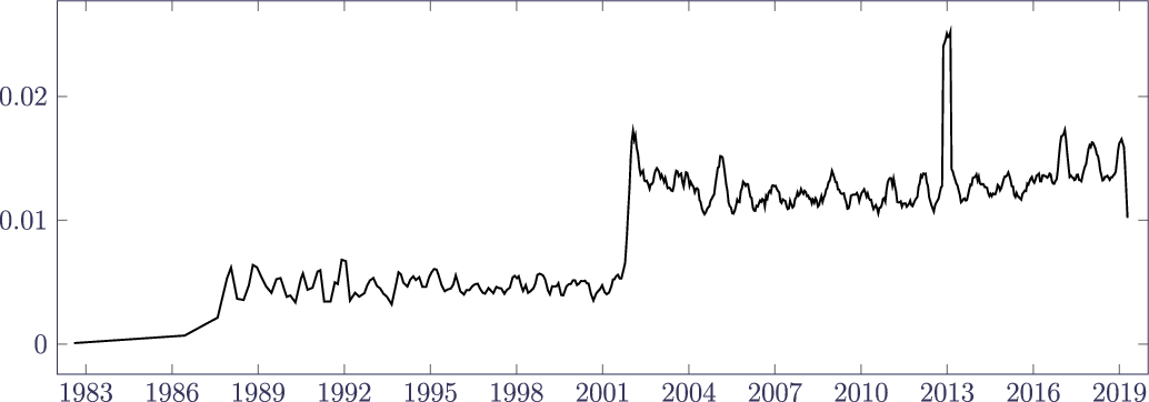
Figure A.1. shows that the June 2019 extract for the FRA portfolio in Table 1 has three phases: (i) some sparse deaths data for a period up to around 1987 that clearly cannot be used for mortality analysis, (ii) a period of stable experience over 1988–2001, and (iii) a period post-2002 also with stable experience, but with a far higher mortality level. The first question is what caused the jump between the second and third phases? We could be dealing with a portfolio that was merged with another portfolio with a substantially higher age, or else the removal of a block of annuities with higher average age as in Figure 1 for UK3. However, in this case the policy counts represented by
 $l_{y+t_i^-}$
(not shown) demonstrate steady growth and no discontinuity, which means that the 1988–2001 phase of experience data must be systematically missing death records, regardless of its apparent stability. The estimator in equation (2) reveals the usable part of the exposure period to be post-2002 for the FRA portfolio.
Plot of
 $\hat\mu_{1982+t}$
using June 2019 extract for FRA portfolio in Table 1. Source: own calculations using equation (2) with
 $c=0.3$
. Only the period from 2002 onwards has complete death data for analysis, although the spike at the start of 2013 suggests some invalidly processed deaths.

The spike in mortality level at the start of 2013 in Figure A.1 is also of interest. This was traced to 670 “deaths” on 1 January 2013, which was clearly not the actual date of death for these annuitants. This sort of data issue would also be caught by the tabulation of the most commonly occurring field values (Macdonald et al., Reference Macdonald, Richards and Currie2018, Section 2.7). However, the estimator in equation (2) provides a clear visual indicator that something is amiss with the data at the start of 2013.
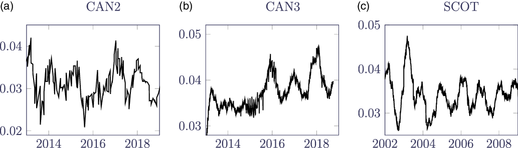
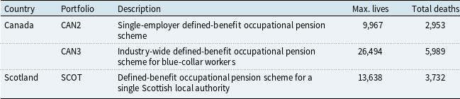
The estimator in equation (2) can also highlight periods of potentially suspect data beyond the two examples in Figure A.1 Table A.1 summarises the data available for three medium-sized pension schemes, while Figure A.2 shows the estimator in equation (2) for each. Figure A.2(a) shows what happens when the dates of death are not accurately recorded – the unclear signal is due to most deaths for CAN2 being recorded as happening in the middle of each month, rather than on the actual date of death. Figure A.2(b) shows that the expected seasonal pattern is present for CAN3 in 2016–2019, but that it is missing from late 2013 to early 2015; the record counts are consistent and have no discontinuity (not shown), so something is probably amiss with the death recording prior to mid-2015. In contrast, Figure A.2(c) shows a reliable seasonal pattern for the SCOT portfolio, indicating that the data have no obvious time-based issues.
Plot of
 $\hat\mu_{2013+t}$
for CAN2 and CAN3 portfolios and
 $\hat\mu_{2002+t}$
for SCOT in Table A.1. Source: own calculations using equation (2) with
 $c=0.5$
. The lack of a clear signal for CAN2 is caused by most deaths being logged as occurring in the middle of the month. The CAN3 portfolio is missing the expected seasonal pattern from late 2013 to early 2015, raising questions over the accuracy of the experience data during that period. In contrast, the SCOT portfolio has a clear recurring seasonal signal throughout, indicating that the data have no obvious time-based issues for the period shown.

Overview of three medium-sized pension schemes, none of which contains mortality experience including the COVID-19 pandemic. The naming convention is consistent with Richards et al. (Reference Richards, Ramonat, Vesper and Kleinow2020), who use two of the same portfolios.

Section 2 highlighted the challenge in validating experience data when certain fields are missing due to data-protection and privacy laws. However, the estimator in equation (2) requires no personal data for its computation. There is therefore no reason for a risk cedant not to share the minimum data fields required, making equation (2) a useful data-quality check in an environment of strict data protection and privacy.
B. Parameters
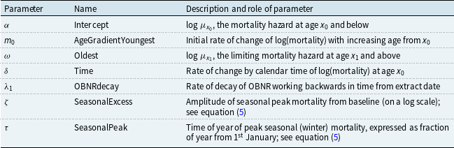
There are two kinds of parameters for a Hermite-spline model (Richards, 2020) of mortality: (i) configuration parameters, whose values are decided in advance by the analyst, and (ii) parameters whose values are estimated from the data.
B.1 Parameters set by the analyst
Table B.1 sets out the configuration parameters set in advance by the analyst, i.e. they are not estimated from the data. The values used in the main body of the paper are given.
Configuration parameters for the Hermite model family.

In addition, the analyst must also choose an OBNR function from equations (5)–(10).
B.2 Parameters estimated from the data
Table B.2 sets out the parameters whose values are estimated from the data by maximum likelihood.
Overview of seasonal and OBNR parameters.

B.3 Parameter correlations
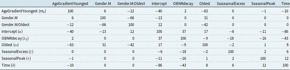
Confounding is a potential issue with the parametric model in section 5. Under normal circumstances, a parametric OBNR term may be confounded with seasonal effects. For this reason we should include a seasonal term in an OBNR model, as per equation (11). However, the data extracts for the FRA and UK3 portfolios were also taken at a time of dramatic short-term changes in mortality levels caused by COVID-19, so there remains potential for confounding even with a seasonal mortality model. Table B.3 shows the percentage correlations between the parameters for the best-fitting OBNR model fitted to the FRA data set (this being the portfolio with the most pronounced OBNR effect). The OBNRdecay estimate,
 $\hat\lambda_1$
, has a strong negative correlation of
 $-43\%$
with the time trend,
 $\delta$
, albeit this correlation is not as strong as some other parameter pairings.
Percentage correlations between parameter estimates in the model in Table 4 fitted to FRA data with an AIC of 164,008. Of note is the absence of any correlation between gender and any of OBNR, season or time trend.

Another question is the robustness of the correlations in Table B.3. Table B.4 shows the correlations between OBNRdecay and other parameter estimates when varying the length of the exposure period. The estimate and standard error of the OBNR decay parameter
 $\lambda_1$
are both robust to the length of the exposure period: from 1.3442 (s.e. 0.0532) with 4.5 years to 1.33501 (s.e. 0.0479) with 8.5 years of experience data (with
 $\hat\lambda_1=1.32332$
(s.e. 0.0508) using 5.5 years as in the main body of the paper).
Percentage correlations between OBNRdecay (
 $\hat\lambda_1$
) and other parameter estimates with varying exposure periods. FRA portfolio with June 2020 extract, Gaussian OBNR function from equation (8).

C. R Code for Semi-parametric Estimator
# Bandwidth parameter for equation (2).
c <- 0.5
# Read in CSV data file with (i) calendar time, (ii) lives (or policies) and
# (iii) deaths (or cessations). Rows are assumed sorted by ascending time.
d <- read.csv(file="SCOT_April_2010.csv”, header=TRUE, skip=1)
# Calculate Nelson-Aalen cumulative hazard in time as per equation (1).
d$NelsonAalen <- cumsum(d$Deaths/d$Lives)
# Calculate smoothed hazard in time as per equation (2).
n <- length(d$Time)
d$Mu <- rep(NA, n)
for (y in 2:n)
{
interval <- findInterval(c(d$Time[y]-c/2, d$Time[y]+c/2), d$Time)
if (interval[1]*interval[2] > 0)
d$Mu[y] <- (d$NelsonAalen[interval[2]] - d$NelsonAalen[interval[1]])/c
}
# Plot Nelson-Aalen cumulative hazard and c-smoothed hazard as per Figure 2.
par(mfrow=c(1,2), mar=c(2, 3, 0, 0))
plotter <- function(time, response, label)
{
plot(time, response, xlim=range(2001, 2009), type="n”, axes=FALSE, xlab="”, ylab="”)
axis(1, las=1)
axis(2, las=1)
lines(time, response)
legend(“bottomright”, legend=label, bty="n”)
}
plotter(d$Time, d$NelsonAalen, “Nelson-Aalen estimate”)
plotter(d$Time, d$Mu, paste0(“Hazard estimate with c=”, c))