




1 Introduction
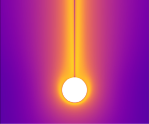
A spherical particle sinking at intermediate Reynolds number through a chemical gradient draws fluid downward, disturbing the local composition field without generating turbulence. If the diffusivity of the chemical is small compared to the particle’s size and speed, the particle leaves behind a trail in which the chemical gradient is intensified in some regions and weakened in others. This gradient deformation is evident in figure 1, modified from Yick et al. (Reference Yick, Torres, Peacock and Stocker2009), which shows a microscale schlieren image of a sphere sinking at low Reynolds number in a salinity-stratified tank. The schlieren technique visualizes changes in the background linear density gradient; here the gradient is enhanced around the sphere and in two tracks that extend 20 sphere diameters downstream. Variation in the gradient across chemical isosurfaces must also result in changes in the diffusive flux in the vicinity of the trail. Yick et al. (Reference Yick, Torres, Peacock and Stocker2009) focused on the increased drag on a sphere due to stratification and did not characterize gradients in the trail or the diffusive flux.
A number of studies have depicted disturbance of stratification by falling spheres in order to describe increased drag (Eames & Hunt Reference Eames and Hunt1997; Srdić-Mitrović, Mohamed & Fernando Reference Srdić-Mitrović, Mohamed and Fernando1999; Yick et al. Reference Yick, Torres, Peacock and Stocker2009; Zhang, Mercier & Magnaudet Reference Zhang, Mercier and Magnaudet2019; Magnaudet & Mercier Reference Magnaudet and Mercier2020), settling speed anomalies (Abaid et al. Reference Abaid, Adalsteinsson, Agyapong and McLaughlin2004; Camassa et al. Reference Camassa, Falcon, Lin, McLaughlin and Parker2009, Reference Camassa, Falcon, Lin, McLaughlin and Mykins2010, Reference Camassa, Khatri, McLaughlin, Prairie, White and Yu2013; Doostmohammadi, Dabiri & Ardekani Reference Doostmohammadi, Dabiri and Ardekani2014), internal wave generation (Mowbray & Rarity Reference Mowbray and Rarity1967) and buoyant jets behind the sphere (Ochoa & Van Woert Reference Ochoa and Van Woert1977; Torres et al. Reference Torres, Hanazaki, Ochoa, Castillo and Van Woert2000; Hanazaki, Kashimoto & Okamura Reference Hanazaki, Kashimoto and Okamura2009a; Hanazaki, Konishi & Okamura Reference Hanazaki, Konishi and Okamura2009b; Hanazaki, Nakamura & Yoshikawa Reference Hanazaki, Nakamura and Yoshikawa2015). These studies indicate that perturbations of the compositional field by a sphere depend on viscosity, diffusivity and buoyancy, which we parameterize by the Reynolds number  $Re=Wl/\unicode[STIX]{x1D708}$, the Péclet number
 $\mathit{Pe}=ReSc=Wl/\unicode[STIX]{x1D705}$ and the Froude number
 $\mathit{Fr}=W/Na$, where
 $W$ is the velocity of the sphere,
 $l$ is the sphere diameter,
 $a$ is the sphere radius,
 $\unicode[STIX]{x1D708}$ is the kinematic viscosity,
 $\unicode[STIX]{x1D705}$ is the diffusivity,
 $N$ is the Brunt–Väisälä frequency and
 $Sc=\unicode[STIX]{x1D708}/\unicode[STIX]{x1D705}$ is the Schmidt number. The purpose of this work is to quantify gradient deformation and diffusive flux enhancement by a sphere descending through a general chemical gradient in terms of the Reynolds, Froude and Péclet numbers. At low
 $\mathit{Fr}$, disturbance of the compositional gradient generates buoyancy forces, but when
 $\mathit{Fr}$ is sufficiently large, buoyancy forces are negligible and the chemical behaves as a passive, diffusive substance advected by the sphere. Both cases are examined in this work.
Alteration of diffusive fluxes by gradient deformation is relevant to any system with objects moving through inhomogeneities at low to intermediate Reynolds numbers, such as particles sinking in the ocean and atmosphere. Sinking detritus and swimming plankton drag fluid and may generate small-scale fluxes of nutrients and other chemicals important for microscale ocean ecology (Katija & Dabiri Reference Katija and Dabiri2009; Noss & Lorke Reference Noss and Lorke2014; Wang & Ardekani Reference Wang and Ardekani2015; Houghton & Dabiri Reference Houghton and Dabiri2019), although there is some debate as to whether plankton mix vertical stratification at large scales (Dewar et al. Reference Dewar, Bingham, Iverson, Nowacek, St. Laurent and Wiebe2006; Visser Reference Visser2007; Houghton et al. Reference Houghton, Koseff, Monismith and Dabiri2018). Dust and bacteria are ubiquitous in the atmosphere and act as a substrate for ice nucleation and cloud formation (DeMott et al. Reference DeMott, Sassen, Poellot, Baumgardner, Rogers, Brooks, Prenni and Kreidenweis2003; Bowers et al. Reference Bowers, Lauber, Wiedinmyer, Hamady, Hallar, Fall, Knight and Fierer2009). Microscale stirring by these particles could influence nucleation rates and factor into the ecology of airborne bacteria (Grover & Pruppacher Reference Grover and Pruppacher1985; Lighthart Reference Lighthart1997). Another potential application concerns the precipitation of heavy solids at the top of terrestrial planetary cores. Falling iron generates convective motions that have been linked to the generation of the ancient magnetic fields of the Moon (Laneuville et al. Reference Laneuville, Wieczorek, Breuer, Aubert, Morard and Rückriemen2014) and Mars (Davies & Pommier Reference Davies and Pommier2018) and the present magnetic field of Ganymede (Rückriemen, Breuer & Spohn Reference Rückriemen, Breuer and Spohn2015). The influence of this ‘iron snow’ on background stratification in the planetary core is not known but may affect the nature and vigour of convection.
The factors that characterize the extent of gradient deformation are the thickness of the chemical boundary layer  $\unicode[STIX]{x1D6FF}_{\unicode[STIX]{x1D70C}}$, the distance over which chemical isosurfaces are dragged
 $\mathit{L}_{Def}$, the chemical flux through the boundary layer
 $\mathit{Sh}$ and a new quantity
 $\mathit{M}$ describing the Lagrangian flux.
Microscale schlieren image of a sphere sinking through salinity stratification for  $Re\approx 2$,
 $\mathit{Fr}\approx 10$ and
 $\mathit{Pe}\approx 10^{3}$ (reproduced from Yick et al. (Reference Yick, Torres, Peacock and Stocker2009)). The greyscale intensity indicates the absolute value of the magnitude of the gradient of the salinity anomaly. Superimposed curves are isosurfaces of salinity from our simulation using equivalent parameters. The scale bar is 3 mm.

Deformation of a plane of dye by a sphere was first described by Darwin (Reference Darwin1953), who derived the position of dye particles in potential flow after the sphere travelled an infinite distance. Lighthill (Reference Lighthill1956) found asymptotic solutions for the location of the dye at finite times during the passage of the sphere. For a sphere moving through a linear gradient of dye, the positions of a single dye isosurface at time increments  $\unicode[STIX]{x0394}t$ are equivalent to isosurfaces of the dye field at concentration increments
 $\unicode[STIX]{x0394}\unicode[STIX]{x1D70C}$, in the frame of reference of the sphere. Eames & Hunt (Reference Eames and Hunt1997) used this equivalence to calculate the composition and flow fields for a sphere moving in weak stratification at high
 $Re$. In the absence of diffusion, isosurfaces pile up at the stagnation point upstream of the sphere as they are stretched infinitely far. The composition and its gradient are then singular on the surface of the sphere, which they predicted would generate a downstream jet.
Numerical simulations conducted by Torres et al. (Reference Torres, Hanazaki, Ochoa, Castillo and Van Woert2000) for  $Re>25$ demonstrated that stratification collapses the standing vortices that normally appear in the wake of a sphere, and the displaced isosurfaces generate a buoyant jet on their return. In addition to confirming the prediction from Eames & Hunt (Reference Eames and Hunt1997), they showed that diffusion allows the sphere to pass through isosurfaces so that they are only dragged a finite distance, allowing steady solutions to be found. The maximum vertical distance an isosurface can be dragged,
 $\mathit{L}_{Def}$, is correlated with the extent of gradient deformation, as we will show later. Hanazaki et al. (Reference Hanazaki, Nakamura and Yoshikawa2015) employed a dimensional analysis of the buoyancy time scale to estimate this distance as
 $l\unicode[STIX]{x03C0}\mathit{Fr}$ for
 $Re\geqslant 200$,
 $1\leqslant \mathit{Fr}\leqslant 10$ and
 $Pe>10^{5}$. Yick et al. (Reference Yick, Torres, Peacock and Stocker2009) combined experiments and numerical results to empirically estimate the dragged distance as
 $l\sqrt{\mathit{Fr}}$ for
 $Re<1$,
 $\mathit{Fr}<1$ and
 $\mathit{Pe}<10^{3}$. Both they and Hanazaki et al. (Reference Hanazaki, Konishi and Okamura2009b) suggested that
 $\mathit{L}_{Def}$ should increase with decreasing diffusivity, but neither provided
 $\mathit{Sc}$ or
 $\mathit{Pe}$ scalings.
Compositional isosurfaces that are dragged downward by the sphere constitute a chemical boundary layer near the surface that is analogous to the classic problem of mass transfer from a sphere. For  $Re\rightarrow \infty$ and
 $Sc\rightarrow 0$, the thickness of the chemical boundary layer is described by
 $\unicode[STIX]{x1D6FF}_{\unicode[STIX]{x1D70C}}/l\sim \mathit{Pe}^{-1/2}$ (Schlichting Reference Schlichting1968; Yih Reference Yih1969). Previous studies of spheres sinking through salinity gradients have used this relation to justify the grid spacing in their numerical models but noted that it underestimates the chemical boundary layer thickness for finite
 $Re$ and
 $\mathit{Sc}$ (Torres et al. Reference Torres, Hanazaki, Ochoa, Castillo and Van Woert2000; Hanazaki et al. Reference Hanazaki, Kashimoto and Okamura2009a, Reference Hanazaki, Nakamura and Yoshikawa2015; Doostmohammadi et al. Reference Doostmohammadi, Dabiri and Ardekani2014). In this work, we derive a new scaling for
 $\unicode[STIX]{x1D6FF}_{\unicode[STIX]{x1D70C}}$ in the
 $10^{-2}\leqslant Re\leqslant 10^{2}$ and
 $\mathit{Pe}>10$ regime. We show that this scaling is critical for determining
 $\mathit{L}_{Def}$,
 $\mathit{Sh}$ and
 $\mathit{M}$.
Here we present a combined analytical and numerical study of gradient deformation and diffusive flux enhancement by a sphere descending through a linear chemical gradient. Methods are detailed in § 2. In § 3.1, we describe the general process of gradient deformation with a representative case and define the quantities  $\unicode[STIX]{x1D6FF}_{\unicode[STIX]{x1D70C}}$,
 $\mathit{L}_{Def}$,
 $Sh$ and
 $\mathit{M}$ that are used in the subsequent analysis to characterize the influence of diffusion (§ 3.2), viscosity (§ 3.3) and buoyancy (§ 3.4). Previous work on spheres sinking through salinity gradients has focused on
 $Re\geqslant 200$ or
 $Re<10$,
 $Fr<10$ and
 $Sc=7,700$ (Torres et al. Reference Torres, Hanazaki, Ochoa, Castillo and Van Woert2000; Yick et al. Reference Yick, Torres, Peacock and Stocker2009; Hanazaki et al. Reference Hanazaki, Nakamura and Yoshikawa2015). The parameter range considered here is
 $10^{-2}\leqslant Re\leqslant 10^{2}$,
 $10^{-1}\leqslant \mathit{Fr}\leqslant 10^{3}$ and
 $10^{2}<\mathit{Pe}\leqslant 10^{6}$. This regime is relevant to particles and plankton in the ocean. The potential for sinking ocean particles to deform ambient chemical gradients is discussed in § 4.
2 Methods
2.1 Governing equations
We consider a sphere sinking through a linear, vertical gradient of a diffusive chemical, such as the nutrient nitrate in the upper ocean. At low Froude numbers, disturbance of the compositional gradient induces buoyancy forces. When  $\mathit{Fr}\geqslant 10^{3}$, buoyancy forces are negligible and the sphere can then be envisioned as travelling in the direction of a gradient of passive, dilute chemical. Both cases are examined in this work and explicit reference to the Froude number is made to distinguish them. In the stationary reference frame of a sphere falling with speed
 $W$, the dimensional forms of the governing equations are
 $$\begin{eqnarray}\displaystyle & \displaystyle \unicode[STIX]{x1D70C}\frac{\text{D}\boldsymbol{u}}{\text{D}t}=-\unicode[STIX]{x1D735}p-\unicode[STIX]{x1D70C}g\,\hat{\boldsymbol{z}}+\unicode[STIX]{x1D707}\unicode[STIX]{x1D6FB}^{2}\boldsymbol{u}, & \displaystyle\end{eqnarray}$$
 $$\begin{eqnarray}\displaystyle & \displaystyle \frac{\text{D}\unicode[STIX]{x1D70C}}{\text{D}t}=\unicode[STIX]{x1D705}\unicode[STIX]{x1D6FB}^{2}\unicode[STIX]{x1D70C} & \displaystyle\end{eqnarray}$$
and
 $$\begin{eqnarray}\unicode[STIX]{x1D735}\boldsymbol{\cdot }\boldsymbol{u}=0,\end{eqnarray}$$
where  $\unicode[STIX]{x1D70C}$ is the density of the fluid,
 $t$ is time,
 $\boldsymbol{u}$ is the velocity vector,
 $p$ is the pressure,
 $g$ is the acceleration due to gravity,
 $\unicode[STIX]{x1D707}$ is the dynamic viscosity of the fluid and
 $\unicode[STIX]{x1D705}$ is the diffusivity coefficient of the chemical. The Boussinesq approximation is used and it is assumed that variation in
 $\unicode[STIX]{x1D70C}$ is due to differences in chemical concentration alone. Therefore spatial gradients of
 $\unicode[STIX]{x1D70C}$ are referred to as chemical gradients. The flow is assumed to be axisymmetric and so
 $\hat{\boldsymbol{z}}$ is the unit vector in the direction of the vertical axis of symmetry and
 $\boldsymbol{u}=(u,w)$, with
 $u$ the radial and
 $w$ the vertical components of velocity in cylindrical coordinates. Laboratory experiments with spheres descending through both stratified and unstratified fluids have exhibited axisymmetric flow patterns when
 $Re<200$ (Taneda Reference Taneda1956; Ochoa & Van Woert Reference Ochoa and Van Woert1977; Yick et al. Reference Yick, Torres, Peacock and Stocker2009; Hanazaki et al. Reference Hanazaki, Kashimoto and Okamura2009a; Okino, Akiyama & Hanazaki Reference Okino, Akiyama and Hanazaki2017).
Numerical simulations are conducted in the reference frame of the sphere such that isosurfaces of chemical appear to move upward past the sphere at constant speed  $W$. The background, unperturbed chemical field and hydrostatic pressure are functions of
 $z$ and
 $t$:
 $$\begin{eqnarray}\bar{\unicode[STIX]{x1D70C}}(z,t)=\unicode[STIX]{x1D70C}_{0}+\frac{\unicode[STIX]{x2202}\bar{\unicode[STIX]{x1D70C}}}{\unicode[STIX]{x2202}z}(z-Wt)\end{eqnarray}$$
and
 $$\begin{eqnarray}\bar{p}(z,t)=-\int \bar{\unicode[STIX]{x1D70C}}(z,t)g\,\text{d}z,\end{eqnarray}$$
where  $\unicode[STIX]{x2202}\bar{\unicode[STIX]{x1D70C}}/\unicode[STIX]{x2202}z$ is the undisturbed vertical gradient of chemical and
 $\unicode[STIX]{x1D70C}_{0}$ is a reference value of the total fluid density at
 $z=0$ and
 $t=0$.
The total density and total pressure are decomposed into the background states and respective perturbations  $\unicode[STIX]{x1D70C}^{\prime }$ and
 $p^{\prime }$:
 $$\begin{eqnarray}\unicode[STIX]{x1D70C}=\bar{\unicode[STIX]{x1D70C}}(z,t)+\unicode[STIX]{x1D70C}^{\prime }(r,z,t)\end{eqnarray}$$
and
 $$\begin{eqnarray}p=\bar{p}(z,t)+p^{\prime }(r,z,t).\end{eqnarray}$$
Substituting the  $\unicode[STIX]{x1D70C}$ and
 $p$ decompositions in (2.6) and (2.7) into (2.1), subtracting the background state and applying the Boussinesq approximation produce
 $$\begin{eqnarray}\frac{\text{D}\boldsymbol{u}}{\text{D}t}=-\frac{1}{\unicode[STIX]{x1D70C}_{0}}\unicode[STIX]{x1D735}p^{\prime }-\frac{\unicode[STIX]{x1D70C}^{\prime }}{\unicode[STIX]{x1D70C}_{0}}g\,\hat{\boldsymbol{z}}+\unicode[STIX]{x1D708}\unicode[STIX]{x1D6FB}^{2}\boldsymbol{u},\end{eqnarray}$$
where  $\unicode[STIX]{x1D708}=\unicode[STIX]{x1D707}/\unicode[STIX]{x1D70C}_{0}$ is the kinematic viscosity. A similar substitution of (2.6) into (2.2) gives
 $$\begin{eqnarray}\frac{\text{D}\unicode[STIX]{x1D70C}^{\prime }}{\text{D}t}=-\frac{\unicode[STIX]{x2202}\bar{\unicode[STIX]{x1D70C}}}{\unicode[STIX]{x2202}z}(w-W)+\unicode[STIX]{x1D705}\unicode[STIX]{x1D6FB}^{2}\unicode[STIX]{x1D70C}^{\prime }.\end{eqnarray}$$
The non-dimensional forms of (2.8) and (2.9) are obtained by scaling distances by the diameter of the sphere  $l=2a$, velocities by the background flow
 $W$, pressure perturbation by
 $\unicode[STIX]{x1D70C}_{0}W^{2}$ and chemical perturbation by
 $-l(\unicode[STIX]{x2202}\bar{\unicode[STIX]{x1D70C}}/\unicode[STIX]{x2202}z)$ as follows:
 $$\begin{eqnarray}\frac{\text{D}\boldsymbol{u}}{\text{D}t}=-\unicode[STIX]{x1D735}p^{\prime }-\frac{4}{\mathit{Fr}^{2}}\unicode[STIX]{x1D70C}^{\prime }\hat{\boldsymbol{z}}+\frac{1}{\mathit{Re}}\unicode[STIX]{x1D6FB}^{2}\boldsymbol{u}\end{eqnarray}$$
and
 $$\begin{eqnarray}\frac{\text{D}\unicode[STIX]{x1D70C}^{\prime }}{\text{D}t}=w-1+\frac{1}{\mathit{Pe}}\unicode[STIX]{x1D6FB}^{2}\unicode[STIX]{x1D70C}^{\prime }.\end{eqnarray}$$
The non-dimensional parameters in (2.10) and (2.11) are the Froude number  $\mathit{Fr}=W/Na$, Reynolds number
 $Re=Wl/\unicode[STIX]{x1D708}$ and Péclet number
 $\mathit{Pe}=Wl/\unicode[STIX]{x1D705}$, where
 $N$ is the Brunt–Väisälä frequency defined by
 $$\begin{eqnarray}N^{2}=-\frac{g}{\unicode[STIX]{x1D70C}_{0}}\frac{\unicode[STIX]{x2202}\bar{\unicode[STIX]{x1D70C}}}{\unicode[STIX]{x2202}z}.\end{eqnarray}$$
When  $\mathit{Fr}$ is small,
 $\unicode[STIX]{x1D70C}^{\prime }$ enters the momentum equation (2.10) through the buoyancy term, and disturbance of the chemical gradient generates buoyancy forces. When
 $\mathit{Fr}\geqslant 10^{3}$, the buoyancy term is negligible compared to the other terms for the parameter range studied and
 $\unicode[STIX]{x1D70C}^{\prime }$ no longer has an influence on the momentum equation (i.e. (2.10) and (2.11) are decoupled). This is confirmed by comparing
 $\mathit{Fr}=10^{3}$ simulations to test cases where the buoyancy term is set to zero. Therefore,
 $\unicode[STIX]{x1D70C}^{\prime }$ signifies a passive, dilute substance at
 $\mathit{Fr}=10^{3}$. In this case,
 $\unicode[STIX]{x1D70C}^{\prime }$ diffuses away over time through the last term in (2.11) because
 $w-1\rightarrow 0$ away from the sphere and
 $\unicode[STIX]{x1D70C}^{\prime }=0$ is the background state (2.6) which is enforced on the outer boundary as described below. In other words, diffusion allows the chemical field to assume its background state following a perturbation, in the absence of buoyancy forces.
Because (2.3), (2.10) and (2.11) do not explicitly include the time development of pressure, we employ a diagnostic Poisson equation for pressure. Taking the divergence of (2.10) gives
 $$\begin{eqnarray}\unicode[STIX]{x1D6FB}^{2}p^{\prime }=-\frac{4}{\mathit{Fr}^{2}}\unicode[STIX]{x1D735}\boldsymbol{\cdot }(\unicode[STIX]{x1D70C}^{\prime }\hat{\boldsymbol{z}})-\unicode[STIX]{x1D735}\boldsymbol{\cdot }[(\boldsymbol{u}\boldsymbol{\cdot }\unicode[STIX]{x1D735})\boldsymbol{u}]+\frac{1}{\mathit{Re}}\unicode[STIX]{x1D6FB}^{2}D-\frac{\unicode[STIX]{x2202}D}{\unicode[STIX]{x2202}t},\end{eqnarray}$$
where  $D=\unicode[STIX]{x1D735}\boldsymbol{\cdot }\boldsymbol{u}$. The time discretization of the diagnostic pressure equation satisfies the divergence-free requirement in (2.3), as described in the next section.
Boundary conditions on the surface of the sphere ( $z^{2}+r^{2}=a^{2}$) are no-slip and no chemical flux:
 $$\begin{eqnarray}\boldsymbol{u}=(u,w)=(0,0)\end{eqnarray}$$
and
 $$\begin{eqnarray}\unicode[STIX]{x1D735}\unicode[STIX]{x1D70C}\boldsymbol{\cdot }\hat{\boldsymbol{n}}=0,\end{eqnarray}$$
where  $\hat{\boldsymbol{n}}$ is the unit vector normal to the sphere surface. The non-dimensional form of the no-flux boundary condition (2.14) is
 $$\begin{eqnarray}z\frac{\unicode[STIX]{x2202}\unicode[STIX]{x1D70C}^{\prime }}{\unicode[STIX]{x2202}z}+r\frac{\unicode[STIX]{x2202}\unicode[STIX]{x1D70C}^{\prime }}{\unicode[STIX]{x2202}r}=z.\end{eqnarray}$$
Inserting (2.13) into (2.10), the boundary condition for pressure on the surface of the sphere becomes
 $$\begin{eqnarray}\unicode[STIX]{x1D735}p^{\prime }=-\frac{4}{\mathit{Fr}^{2}}\unicode[STIX]{x1D70C}^{\prime }\hat{\boldsymbol{z}}+\frac{1}{\mathit{Re}}\unicode[STIX]{x1D6FB}^{2}\boldsymbol{u}.\end{eqnarray}$$
Physical quantities are assumed to asymptote to their unperturbed values far from the sphere because of viscosity, diffusivity and geometrical spreading effects. Accordingly, the compositional perturbation is extinguished on the outer edge of the computed domain
 $$\begin{eqnarray}\unicode[STIX]{x1D70C}^{\prime }=0\end{eqnarray}$$
and a zero normal derivative is enforced for the pressure
 $$\begin{eqnarray}\frac{\unicode[STIX]{x2202}p^{\prime }}{\unicode[STIX]{x2202}n}=0.\end{eqnarray}$$
Entering the upstream (lower) boundary, velocities are fixed as
 $$\begin{eqnarray}\boldsymbol{u}=(u,w)=(0,1)\end{eqnarray}$$
and exiting the downstream (upper) boundary, the velocities are extrapolated assuming no vertical derivative
 $$\begin{eqnarray}\frac{\unicode[STIX]{x2202}u}{\unicode[STIX]{x2202}z}=\frac{\unicode[STIX]{x2202}w}{\unicode[STIX]{x2202}z}=0.\end{eqnarray}$$
2.2 Numerical methods
The numerical methods used to solve (2.10)–(2.12) are based on Torres et al. (Reference Torres, Hanazaki, Ochoa, Castillo and Van Woert2000) and Yick et al. (Reference Yick, Torres, Peacock and Stocker2009). Solutions for the pressure, velocities and chemical concentration are calculated each time step on a computational grid using finite differences with the marker and cell (MAC) method (Harlow & Welch Reference Harlow and Welch1965). The MAC method has been modified for incompressible stratified fluids (Hanazaki Reference Hanazaki1988) and density diffusion (Torres et al. Reference Torres, Hanazaki, Ochoa, Castillo and Van Woert2000), and is adjusted here for  $Re<200$ and chemical gradients with diminishing buoyancy forces.
The time evolution of the flow is discretized using an explicit Euler method. Dropping the primes that denote non-dimensional variables for clarity in this section only, equations (2.10)–(2.12) are rewritten as
 $$\begin{eqnarray}\displaystyle & \displaystyle \frac{\boldsymbol{u}^{n+1}-\boldsymbol{u}^{n}}{\unicode[STIX]{x0394}t}+(\boldsymbol{u}^{n}\boldsymbol{\cdot }\unicode[STIX]{x1D735})\boldsymbol{u}^{n}=-\unicode[STIX]{x1D735}p^{n}-\frac{4}{\mathit{Fr}^{2}}\unicode[STIX]{x1D70C}^{n}\hat{\boldsymbol{z}}+\frac{1}{\mathit{Re}}\unicode[STIX]{x1D6FB}^{2}\boldsymbol{u}^{n}, & \displaystyle\end{eqnarray}$$
 $$\begin{eqnarray}\displaystyle & \displaystyle \frac{\unicode[STIX]{x1D70C}^{n+1}-\unicode[STIX]{x1D70C}^{n}}{\unicode[STIX]{x0394}t}+(\boldsymbol{u}^{n}\boldsymbol{\cdot }\unicode[STIX]{x1D735})\unicode[STIX]{x1D70C}^{n}=w^{n}-1+\frac{1}{\mathit{Pe}}\unicode[STIX]{x1D6FB}^{2}\unicode[STIX]{x1D70C}^{n} & \displaystyle\end{eqnarray}$$
and
 $$\begin{eqnarray}\unicode[STIX]{x1D6FB}^{2}p^{n}=-\frac{4}{\mathit{Fr}^{2}}\unicode[STIX]{x1D735}\boldsymbol{\cdot }(\unicode[STIX]{x1D70C}^{n}\hat{\boldsymbol{z}})-\unicode[STIX]{x1D735}\boldsymbol{\cdot }[(\boldsymbol{u}^{n}\boldsymbol{\cdot }\unicode[STIX]{x1D735})\boldsymbol{u}^{n}]+\frac{1}{\mathit{Re}}\unicode[STIX]{x1D6FB}^{2}D^{n}-\frac{D^{n+1}-D^{n}}{\unicode[STIX]{x0394}t},\end{eqnarray}$$
where  $n$ is the current time step corresponding to an integration time of
 $t=n\unicode[STIX]{x0394}t$. The initial condition is an impulsive start in which
 $\unicode[STIX]{x1D70C}=0$,
 $u=0$ and
 $w=W$ everywhere except at the boundary of the sphere where
 $w=0$ as per (2.13). At time step
 $n$, the Poisson equation for pressure (2.23) is solved with given values for
 $\boldsymbol{u}^{n}$ and
 $\unicode[STIX]{x1D70C}^{n}$ using the successive over-relaxation method. In accordance with the MAC method,
 $D^{n+1}$ is set equal to zero to preserve the incompressibility condition (2.3) and
 $D^{n}$ is retained to prevent the accumulation of numerical round-off errors. Inserting
 $p^{n}$ into (2.21),
 $\boldsymbol{u}$ and
 $\unicode[STIX]{x1D70C}$ are then calculated for the next time point
 $n+1$. This process is repeated for each subsequent time step until a steady-state criterion is reached (see § 2.4).
The curvilinear grid used in this study. Every fifth arc and ray are drawn, for clarity. Arcs are clustered towards the sphere to resolve the boundary layer. Rays are clustered towards the downstream axis of symmetry, the positive  $z$ axis. Rays are perpendicular close to the surface of the sphere, and then curve slightly towards the
 $z$ axis to preserve resolution at great distances downstream.

2.3 Curvilinear grid
Equations (2.21)–(2.23) are transformed from the physical plane  $(r,z)$ – represented by the curvilinear grid in figure 2 – to a rectilinear computational domain
 $(\unicode[STIX]{x1D709},\unicode[STIX]{x1D702})$ as described in Torres et al. (Reference Torres, Hanazaki, Ochoa, Castillo and Van Woert2000):
 $$\begin{eqnarray}z=z(\unicode[STIX]{x1D709},\unicode[STIX]{x1D702}),\quad r=r(\unicode[STIX]{x1D709},\unicode[STIX]{x1D702}).\end{eqnarray}$$
A novel curvilinear grid was developed for this work in order to resolve the chemical gradient both near the sphere as well as hundreds of sphere diameters downstream (figure 2). Curvilinear grid rays and arcs correspond to computational coordinates  $\unicode[STIX]{x1D709}$ and
 $\unicode[STIX]{x1D702}$, respectively. As in Torres et al. (Reference Torres, Hanazaki, Ochoa, Castillo and Van Woert2000) and Hanazaki et al. (Reference Hanazaki, Nakamura and Yoshikawa2015), grid arcs (constant
 $\unicode[STIX]{x1D702}$) are clustered towards the sphere to better resolve the thin chemical boundary layer. Using
 $\mathit{Pe}^{-1/2}$ to estimate the thickness of the boundary layer (Schlichting Reference Schlichting1968; Yih Reference Yih1969), the number of grid points in this layer is three for
 $\mathit{Pe}=10^{6}$. The
 $\mathit{Pe}^{-1/2}$ estimate is overly conservative for high Péclet numbers as will be demonstrated in § 3.2. This is comparable to the grid used in Hanazaki et al. (Reference Hanazaki, Nakamura and Yoshikawa2015) for
 $Re=200$ and
 $\mathit{Sc}=700$. Near the sphere, grid rays (constant
 $\unicode[STIX]{x1D709}$) are normal to its surface to accurately implement the no-flux and no-slip boundary conditions on a curve. Rays are clustered towards the forward (upstream) end of the sphere where chemical isosurfaces collect before being punctured by the sphere. As in Hanazaki et al. (Reference Hanazaki, Nakamura and Yoshikawa2015), rays are also clustered towards the rear (downstream) stagnation point to improve resolution of wake structures.
In the large-Péclet-number regime of interest for this study, variation of chemical perturbations is primarily transverse to and concentrated near the  $z$ axis far downstream of the sphere (figure 1). The goal, then, in generating a grid is to maintain high
 $\unicode[STIX]{x1D709}$ resolution transverse to the downstream
 $z$ axis over a very large domain while remaining computationally tractable. Straight rays cause a loss in resolution near the axis of symmetry with increasing
 $z$; instead, at some distance from the sphere the rays are curved from their initial sphere-normal trajectory to become parallel with the
 $z$ axis using a quadratic Bézier scheme. This preserves both
 $\unicode[STIX]{x1D709}$ and
 $\unicode[STIX]{x1D702}$ resolution near the sphere and provides excellent
 $\unicode[STIX]{x1D709}$ resolution at great distances downstream.
The computational grid used in this work is 720  $\unicode[STIX]{x1D709}$ by 1226
 $\unicode[STIX]{x1D702}$ grid points and extends 1200 sphere diameters (
 $l$) to the outer boundary. The smallest grid spacing normal to the sphere is
 $\unicode[STIX]{x0394}\unicode[STIX]{x1D702}=4.39\times 10^{-4}l$. For the extreme case
 $\mathit{Pe}=10^{6}$, there are 25 grid points within a chemical boundary layer of thickness
 $1.89\times 10^{-2}l$, calculated using the method displayed in figure 4. At the downstream edge of the domain ray curvature provides a smallest
 $\unicode[STIX]{x1D709}$ grid spacing of
 $\unicode[STIX]{x0394}\unicode[STIX]{x1D709}=6\times 10^{-3}l$ and 11 grid points within a sphere radius (
 $a$) of the
 $z$ axis. The simulation can run up to a time
 $Wt/2a=1200$ before isosurfaces that started at the sphere reach the boundary. The grid-independence of results is demonstrated in the Appendix.
2.4 Steady state
As the flow develops, the perturbation variables  $u^{\prime }$,
 $w^{\prime }$,
 $p^{\prime }$ and
 $\unicode[STIX]{x1D70C}^{\prime }$ can asymptote towards a steady state after an amount of time that depends on the non-dimensional parameters chosen. All results presented in this work are steady state in the frame of reference of the sphere, meaning that the spatial structure of perturbation variables
 $u^{\prime },w^{\prime },\unicode[STIX]{x1D70C}^{\prime }$ and gradients of total variables such as
 $\unicode[STIX]{x1D735}\unicode[STIX]{x1D70C}$ do not change with time. Because we are interested in the structure of chemical gradients that can propagate hundreds of sphere diameters downstream, simulations are run until a steady-state criterion of
 $|f^{t+1}-f^{t}|_{max}/(f_{max}^{t}-f_{min}^{t})\leqslant 10^{-5}$ is met, where
 $f$ is
 $\unicode[STIX]{x1D735}\unicode[STIX]{x1D70C}\geqslant 0.01\unicode[STIX]{x1D735}\unicode[STIX]{x1D70C}_{max}$. This criterion ensures that 99 % of the gradient structure is steady while simultaneously satisfying
 $|g^{n+1}-g^{n}|_{max}/(g_{max}^{n}-g_{min}^{n})\leqslant 10^{-6}$, where
 $g$ represents
 $\boldsymbol{u}$,
 $p$ and
 $\unicode[STIX]{x1D70C}$ (cf. Torres et al. Reference Torres, Hanazaki, Ochoa, Castillo and Van Woert2000). Simulations with parameters
 $Re\geqslant 10$ and
 $Fr=10^{-1}$ display unsteady, periodic behaviour. These simulations fail the steady-state criterion and are excluded from the results.
Note that the basic chemical field  $\bar{\unicode[STIX]{x1D70C}}(z,t)$ and total fluid density
 $\unicode[STIX]{x1D70C}$ increase linearly with time (equations (2.4) and (2.6)), so that the shapes of all isosurfaces
 $\unicode[STIX]{x1D70C}+(\unicode[STIX]{x2202}\bar{\unicode[STIX]{x1D70C}}/\unicode[STIX]{x2202}z)Wt$ are constant, but the value associated with each advances monotonically. In this way isosurfaces separated by
 $\unicode[STIX]{x0394}\unicode[STIX]{x1D70C}=1$ also represent the time development of a single isosurface with time intervals of
 $\unicode[STIX]{x0394}t=1$ as it moves past the sphere (Hanazaki et al. Reference Hanazaki, Nakamura and Yoshikawa2015). When reference is made to the shape of an isosurface at a given time, the initial time
 $t^{\prime }=Wt/2a=0$ is defined as the time when the portion of the isosurface far from the sphere is located at
 $z=0$.
3 Results
3.1 Deformation of chemical gradients by sinking spheres
We begin by describing deformation of a linear chemical gradient by a sinking sphere and defining the  $\unicode[STIX]{x1D6FF}_{\unicode[STIX]{x1D70C}}$,
 $\mathit{L}_{Def}$,
 $Sh$ and
 $\mathit{M}$ variables that will be used to quantify the influence of diffusivity, viscosity and buoyancy in subsequent sections. For now, we will treat a representative case where the chemical gradient induces negligible buoyancy forces:
 $Re=1$,
 $\mathit{Fr}=10^{3}$ and
 $\mathit{Sc}=\mathit{Pe}=10^{3}$. As explained in § 2.1, equation (2.11) is decoupled from (2.10) at large
 $\mathit{Fr}$ and
 $\unicode[STIX]{x1D70C}$ behaves as a passive chemical subject to diffusion. A dimensional realization of the representative case is a 1 mm diameter particle sinking at
 $1~\text{mm}~\text{s}^{-1}$ through a weak salinity gradient
 $\unicode[STIX]{x2202}\bar{\unicode[STIX]{x1D70C}}/\unicode[STIX]{x2202}z\approx 10^{-4}~\text{kg}~\text{m}^{-4}$ with diffusivity
 $10^{-9}~\text{m}^{2}~\text{s}^{-1}$ in a tank of water with viscosity
 $10^{-6}~\text{m}^{2}~\text{s}^{-1}$. The buoyancy frequency is
 $N=10^{-3}~\text{s}^{-1}$ with gravity
 $g\approx 9.8~\text{m}~\text{s}^{-2}$ and reference density
 $\unicode[STIX]{x1D70C}_{0}=1025~\text{kg}~\text{m}^{-3}$.
A sinking sphere sets the surrounding fluid into motion, dragging isosurfaces of chemical concentration downward (figure 3). An isosurface that began upstream will stretch and wrap around the sphere until the divergence of the concentration gradient reaches a critical threshold  $\unicode[STIX]{x1D6FB}^{2}\unicode[STIX]{x1D70C}^{\prime }=Pe$ (Hanazaki et al. Reference Hanazaki, Nakamura and Yoshikawa2015). This threshold is derived from the steady-state form of (2.11) applied at the sphere surface where
 $(u,w)=0$. Molecular diffusivity then creates a hole in the isosurface at the leading edge of the sphere, which occurs just after
 $t^{\prime }=5$ in this example (figure 3b). As the sphere punches through, the attached portion of the isosurface migrates rearward on the sphere and stretches vertically (figure 3c).
Although there is no flux of material through the surface of the sphere, wrapped isosurfaces form a thin boundary layer next to the sphere (figure 4a). This resembles the concentration boundary layer in the classic problem of mass transfer from a sphere, an analogy that will prove useful for explaining scalings in the next section. The thickness of the chemical boundary layer,  $\unicode[STIX]{x1D6FF}_{\unicode[STIX]{x1D70C}}$, is calculated as shown in figure 4(a). Because the gradient normal to the surface is zero, a line of best fit is drawn at the inflection point of the
 $\unicode[STIX]{x1D70C}^{\prime }$ profile. The intersection of the fitted line and the maximum value of
 $\unicode[STIX]{x1D70C}^{\prime }$ gives the local thickness of
 $\unicode[STIX]{x1D6FF}_{\unicode[STIX]{x1D70C}}$ (Verzicco & Camussi Reference Verzicco and Camussi1999; Breuer et al. Reference Breuer, Wessling, Schmalzl and Hansen2004; Zhou & Xia Reference Zhou and Xia2010). Local values
 $\pm 30^{\circ }$ of the equator are averaged to calculate
 $\unicode[STIX]{x1D6FF}_{\unicode[STIX]{x1D70C}}$, avoiding the region of flow separation when
 $Re\gtrapprox 20$. We also calculated the boundary layer thickness using methods based on percentage of outer
 $\unicode[STIX]{x1D70C}^{\prime }$ (Schlichting Reference Schlichting1968), the inverse of the Sherwood number (Kiørboe, Ploug & Thygesen Reference Kiørboe, Ploug and Thygesen2001) and the second moment of
 $\unicode[STIX]{x1D70C}^{\prime }$ (Weyburne Reference Weyburne2006), and found them all to give similar results. An empirical viscous layer thickness
 $\unicode[STIX]{x1D6FF}_{u}$ is calculated in a similar manner to the chemical boundary layer, as shown in figure 4(b).
Deformation of a chemical isosurface  $S$ by a sphere for
 $Re=1$,
 $\mathit{Fr}=10^{3}$ and
 $\mathit{Pe}=10^{3}$. The colour mapped onto the isosurface is
 $\unicode[STIX]{x1D6FB}^{2}\unicode[STIX]{x1D70C}^{\prime }$. Time is adjusted so that
 $t^{\prime }=0$ when an undisturbed chemical isosurface would have crossed the
 $z=0$ plane. Deformation is shown for (a)
 $t^{\prime }=1$, (b)
 $t^{\prime }=5$ and (c)
 $t^{\prime }=9$.

(a) Profile of local  $\unicode[STIX]{x1D70C}^{\prime }$ outward from the equator, in the
 $n$ direction normal to the surface, for
 $Re=1$,
 $\mathit{Pe}=10^{3}$ and
 $\mathit{Fr}=10^{3}$. The surface of the sphere is located at
 $n=0.5$. Because of the no-flux boundary condition, a line is fitted to the inflection point of
 $\unicode[STIX]{x1D70C}^{\prime }$ (dashed). The intersection of the fitted line and the maximum value of
 $\unicode[STIX]{x1D70C}^{\prime }$ (dotted line) gives the local boundary layer thickness, indicated by the shaded area. The local thickness normal to the sphere averaged within
 $\pm 30^{\circ }$ of the equator is
 $\unicode[STIX]{x1D6FF}_{\unicode[STIX]{x1D70C}}$. (b) Profile of local velocity anomaly parallel to the sphere at the equator. An empirical thickness of the viscous layer is calculated in a similar manner to the calculation of
 $\unicode[STIX]{x1D6FF}_{\unicode[STIX]{x1D70C}}$ using the first 100 grid points for the fitted line.

Simulation of  $Re=1$,
 $\mathit{Fr}=10^{3}$ and
 $\mathit{Pe}=10^{3}$. (a) Isosurfaces of chemical concentration at steady state,
 $\unicode[STIX]{x0394}\unicode[STIX]{x1D70C}=2$. Far from the
 $z$ axis, these isosurfaces are separated by two sphere diameters,
 $\unicode[STIX]{x0394}z=2l$. The isosurface dragged the farthest,
 $\unicode[STIX]{x1D70C}_{Def}$, is indicated by the red dashed line. Here
 $\mathit{L}_{Def}\approx 15$ is the vertical distance from the undisturbed portion of
 $\unicode[STIX]{x1D70C}_{Def}$ far from the
 $z$ axis to the attachment point on the sphere. (b) The change in the magnitude of the chemical gradient from the basic state,
 $G$. (c) The vertical velocity anomaly,
 $w-1$. Bottom panels show the origin and top panels a section 200 sphere diameters downstream.

From initial upstream contact to detachment downstream, a  $\unicode[STIX]{x1D70C}$ isosurface is dragged and deformed by the sphere from its initial unperturbed position to a maximum vertical length
 $\mathit{L}_{Def}$. In this case, this length is
 $\mathit{L}_{Def}\approx 15$ sphere diameters for the isosurface with value
 $\unicode[STIX]{x1D70C}_{Def}=\unicode[STIX]{x1D70C}+(\unicode[STIX]{x2202}\bar{\unicode[STIX]{x1D70C}}/\unicode[STIX]{x2202}z)Wt\approx -15$ (dashed line in figure 5a). After
 $\mathit{L}_{Def}$ is reached, the isosurface either detaches from the rear of the sphere, or pinches off downstream near the sphere and the hole in the isosurface closes. Reformed isosurfaces return to their unperturbed (flat) state at some distance downstream determined by a combination of molecular diffusion and buoyancy, the latter of which is negligible in this case. The slow relaxation of isosurfaces by diffusion is evident 200 sphere diameters downstream where isosurfaces are still vertically deformed by 7 sphere diameters (figure 5, top panel). The entire trail of chemical disturbance is therefore much longer than the maximum deformed distance
 $\mathit{L}_{Def}$.
The magnitude of the chemical gradient  $|\unicode[STIX]{x1D735}\unicode[STIX]{x1D70C}|$ normal to isosurfaces increases above the background state where contours come together and decreases where they spread apart during deformation by the sphere. The deviation of the magnitude of the gradient from the background state is here defined as
 $$\begin{eqnarray}\mathit{G}\equiv \frac{|\unicode[STIX]{x1D735}\unicode[STIX]{x1D70C}|-{\displaystyle \frac{\unicode[STIX]{x2202}\bar{\unicode[STIX]{x1D70C}}}{\unicode[STIX]{x2202}z}}}{{\displaystyle \frac{\unicode[STIX]{x2202}\bar{\unicode[STIX]{x1D70C}}}{\unicode[STIX]{x2202}z}}}.\end{eqnarray}$$
Enhancement of the gradient is visible in the chemical boundary layer and two downstream tracks where the isosurfaces have tilted towards vertical (figure 5a,b). In this case,  $\mathit{G}$ is enhanced by a factor of
 ${\sim}40$ over the background gradient. On the
 $z$ axis, the gradient is reduced from the background state downstream; here isosurfaces pinch off from the sphere and begin to return to their unperturbed state. In three dimensions, the tracks of deformed gradient form a cylindrical plume of gradient enhancement that surrounds a core of gradient reduction. These features stretch for hundreds of sphere diameters downstream until they are erased by diffusion (figure 5, top panel). This gradient deformation trail constitutes a standing structure like a wake, except that it persists to a greater degree in time and space than the velocity perturbations due to large
 $\mathit{Sc}$.
(a) The flow of material,  $F=\int _{S}G\,\text{d}S$, across an isosurface as a function of time. Time
 $t^{\prime }=0$ when the undisturbed portion of the isosurface crosses
 $z=0$. (b) The outer (time) integral of
 $\mathit{M}$, moving from the sphere to the downstream boundary. The line indicates the time when the isosurface has been dragged a distance
 $\mathit{L}_{Def}$.

Gradient enhancement is not balanced by gradient reduction over the course of the deformation event depicted in figure 5. This results in a net increase in the diffusive flux of chemical across isosurfaces that can be evaluated in two ways. Near the sphere, flux through the boundary layer is measured by the Sherwood number:
 $$\begin{eqnarray}\mathit{Sh}=\frac{\displaystyle \frac{1}{A}\int \frac{\unicode[STIX]{x2202}\unicode[STIX]{x1D70C}^{\prime }}{\unicode[STIX]{x2202}n}\,\text{d}A}{\displaystyle \frac{1}{A}\int a^{-1}(\unicode[STIX]{x1D70C}_{\infty }^{\prime }-\unicode[STIX]{x1D70C}_{0}^{\prime })\,\text{d}A},\end{eqnarray}$$
where integration is performed over the surface of the sphere  $A$,
 $\unicode[STIX]{x2202}\unicode[STIX]{x1D70C}^{\prime }/\unicode[STIX]{x2202}n$ is the gradient normal to the sphere surface in the chemical boundary layer (see figure 4a),
 $\unicode[STIX]{x1D70C}_{\infty }^{\prime }=0$ is the value far from the sphere and
 $\unicode[STIX]{x1D70C}_{0}^{\prime }$ is the value at the surface of the sphere (Friedlander Reference Friedlander1957, Reference Friedlander1961; Sherwood, Pigford & Wilke Reference Sherwood, Pigford and Wilke1975; Clift, Grace & Weber Reference Clift, Grace and Weber1978; Karp-Boss, Boss & Jumars Reference Karp-Boss, Boss and Jumars1996). The numerator is the total flux through the thin chemical boundary layer where the velocity becomes vanishingly small at high
 $Sc$. Since there is no flux at the surface, we must calculate the values of
 $\unicode[STIX]{x1D70C}_{0}^{\prime }$ from the simulation. The denominator is the steady-state diffusive flux in the absence of motion. For the case shown in figure 5, the boundary layer flux is increased by a factor of
 $Sh\approx 4$ compared to a stationary sphere.
The total flux including the trail can be calculated in the Lagrangian frame of reference following an isosurface  $S$ that starts upstream, is deformed by the sphere and then returns to an unperturbed state downstream. Note that
 $S$ is the chemical isosurface displayed in figure 3 at different times
 $t^{\prime }$. Because the gradient vector of magnitude
 $\mathit{G}$ is always normal to an isosurface, and because the diffusivity is constant,
 $\mathit{G}$ is proportional to the local net increase or decrease of chemical flux across an isosurface. Integrating
 $\mathit{G}$ over isosurface
 $S$ gives the flow rate
 $F$ of material across the isosurface at a given time,
 $F=\int _{S}G\,\text{d}S$. A time course of
 $F$ following a single isosurface is shown in figure 6(a). The flow rate increases until
 $t^{\prime }=\mathit{L}_{Def}/W$, after which the isosurface is no longer deformed by the sphere and diffusion slowly flattens the isosurface for another
 ${\sim}450$ time units. The total Lagrangian flux is summarized by
 $$\begin{eqnarray}\mathit{M}\equiv \frac{1}{l^{2}T}\int F\,\text{d}t=\frac{1}{l^{2}T}\int _{T}\int _{S}\mathit{G}\,\text{d}S\text{d}t,\end{eqnarray}$$
where  $\mathit{G}$ is integrated over isosurface
 $S$ out to the horizontal edge of the domain and over the time
 $T$ for the isosurface to move from the sphere to the downstream boundary. Because
 $\mathit{G}\rightarrow 0$ away from the deformation trail, the varying width of the curvilinear domain does not influence the calculation. The cumulative outer (time) integral of
 $\mathit{M}$ is shown in figure 6(b). Deformations at times
 $t^{\prime }<\mathit{L}_{Def}/W$ contribute only 12 % of the total
 $\mathit{M}$, which emphasizes the importance of the long trail to the total flux in the system. For the representative case,
 $\mathit{M}$ is an order of magnitude higher than the background, unperturbed state.
To separate the influences of viscosity, diffusivity and buoyancy forces on gradient deformation, we will compare simulations covering combinations of the three-dimensional parameter space  $10^{-2}\leqslant Re\leqslant 10^{2}$,
 $10^{-1}\leqslant \mathit{Fr}\leqslant 10^{3}$ and
 $10\leqslant \mathit{Pe}\leqslant 10^{6}$. The Péclet number was chosen instead of the Schmidt number in order to treat viscous and diffusive effects separately. Over the full parameter space, the variables
 $\unicode[STIX]{x1D6FF}_{\unicode[STIX]{x1D70C}}$,
 $\mathit{L}_{Def}$,
 $Sh$ and
 $\mathit{M}$ show the greatest dependence on the Péclet number. As such, we address the influence of diffusivity on gradient deformation before moving on to viscosity and buoyancy.
3.2 The Péclet number dependence of gradient deformation
In the absence of buoyancy forces ( $\mathit{Fr}\geqslant 10^{3}$), equation (2.11) is decoupled from (2.10) and
 $\unicode[STIX]{x1D70C}$ behaves as a passive chemical. The Péclet number then controls the deformation of chemical isosurfaces and gradients based on the balance of terms in (2.11). We posit that the chemical boundary layer surrounding a sphere sinking through a linear gradient of chemical is analogous to the compositional boundary layer in the classic problem of mass transfer from a falling sphere. The
 $\mathit{Pe}$ dependence of
 $\unicode[STIX]{x1D6FF}_{\unicode[STIX]{x1D70C}}$,
 $\mathit{L}_{Def}$,
 $\mathit{Sh}$ and
 $\mathit{M}$ can be explained using a boundary layer analysis similar to that of the mass transfer problem. As
 $\mathit{Pe}$ increases, the chemical boundary layer near the equator thins (figure 7a). At low
 $\mathit{Pe}$, the
 $w-1$ term of (2.11) is balanced by diffusion and the chemical boundary layer is weak or absent. For
 $\mathit{Pe}>10^{2}$, diffusion is small and the convective term
 $\boldsymbol{u}\boldsymbol{\cdot }\unicode[STIX]{x1D735}\unicode[STIX]{x1D70C}^{\prime }$ dominates, strengthening the gradient normal to the sphere and decreasing
 $\unicode[STIX]{x1D6FF}_{\unicode[STIX]{x1D70C}}$. The thickness of the boundary layer is estimated well by
 $\mathit{Pe}^{-1/3}$ in the high-
 $\mathit{Pe}$ regime (figure 7a). This scaling can be rationalized through dimensional analysis of the chemical boundary layer equation.
(a) The value of  $\unicode[STIX]{x1D6FF}_{\unicode[STIX]{x1D70C}}/l$ as a function of
 $\mathit{Pe}$ for
 $\mathit{Fr}=10^{3}$ and
 $10^{-2}\leqslant Re\leqslant 10^{2}$. The chemical boundary layer thins as
 $Pe$ increases. At large
 $Pe$,
 $\unicode[STIX]{x1D6FF}_{\unicode[STIX]{x1D70C}}/l$ tends towards
 $Pe^{-1/3}$ (dashed line). (b) No such relation exists for the viscous layer thickness versus
 $Re$ for
 $\mathit{Fr}=10^{3}$ and
 $10\leqslant \mathit{Pe}\leqslant 10^{6}$. (c) The terms of the vertical momentum equation (2.10) along streamline
 $\unicode[STIX]{x1D713}=a$ for
 $Re=1$,
 $\mathit{Fr}=10^{3}$ and
 $10\leqslant \mathit{Pe}\leqslant 10^{6}$. The advective terms are subdominant and the pressure gradient is balanced by the viscous term.

At steady state, the chemical distribution very close to the sphere is determined by the standard boundary layer equation with an additional source term:
 $$\begin{eqnarray}u\frac{\unicode[STIX]{x2202}\unicode[STIX]{x1D70C}^{\prime }}{\unicode[STIX]{x2202}x}+v\frac{\unicode[STIX]{x2202}\unicode[STIX]{x1D70C}^{\prime }}{\unicode[STIX]{x2202}n}=\unicode[STIX]{x1D6FE}+\unicode[STIX]{x1D705}\frac{\unicode[STIX]{x2202}^{2}\unicode[STIX]{x1D70C}^{\prime }}{\unicode[STIX]{x2202}n^{2}},\end{eqnarray}$$
where  $u$ is the velocity in the
 $x$ direction parallel to the surface,
 $v$ is the velocity in the
 $n$ direction perpendicular to the surface and the source term
 $\unicode[STIX]{x1D6FE}$ is the dimensional form of
 $w-1$ transformed into the
 $(x,n)$ coordinate system (Landau & Lifshitz Reference Landau and Lifshitz1959; Levich Reference Levich1962; Acrivos & Goddard Reference Acrivos and Goddard1965; Grossmann & Lohse Reference Grossmann and Lohse2000). This is in the frame of reference of the chemical boundary layer, close to the surface of the sphere. The advection, source and diffusion terms are all of the same order of magnitude in the chemical boundary layer for
 $\mathit{Pe}\geqslant 10^{2}$ (figure 8a). We begin our analysis by balancing the advection and diffusion terms.
(a) An equatorial profile of the advection, source and diffusion terms of (2.11) for  $Re=1$,
 $\mathit{Fr}=10^{3}$ and
 $\mathit{Pe}=10^{3}$. The terms are of the same order of magnitude within
 $\unicode[STIX]{x1D6FF}_{\unicode[STIX]{x1D70C}}$, indicated by the shaded area. (b) The velocity parallel to the surface scales as
 $v\sim u\unicode[STIX]{x1D6FF}_{\unicode[STIX]{x1D70C}}/l$ at large
 $\mathit{Pe}$, which confirms that
 $\unicode[STIX]{x2202}u/\unicode[STIX]{x2202}x\sim U\unicode[STIX]{x1D6FF}_{\unicode[STIX]{x1D70C}}/\unicode[STIX]{x1D6FF}_{u}l$ is of the same order of magnitude as
 $\unicode[STIX]{x2202}v/\unicode[STIX]{x2202}n\sim v/\unicode[STIX]{x1D6FF}_{\unicode[STIX]{x1D70C}}$ in the chemical boundary layer. The line represents one-to-one correspondence.

When  $Sc$ is large,
 $\unicode[STIX]{x1D6FF}_{\unicode[STIX]{x1D70C}}<\unicode[STIX]{x1D6FF}_{u}$ and the parallel velocity is estimated by
 $u\sim U\unicode[STIX]{x1D6FF}_{\unicode[STIX]{x1D70C}}/\unicode[STIX]{x1D6FF}_{u}$, where
 $\unicode[STIX]{x1D6FF}_{u}$ is the thickness of the viscous boundary layer and
 $U\sim W$ is the velocity parallel to the surface at
 $\unicode[STIX]{x1D6FF}_{u}$ (Levich Reference Levich1962; Grossmann & Lohse Reference Grossmann and Lohse2000). The incompressibility condition (2.3) requires that
 $\unicode[STIX]{x2202}u/\unicode[STIX]{x2202}x\sim U\unicode[STIX]{x1D6FF}_{\unicode[STIX]{x1D70C}}/\unicode[STIX]{x1D6FF}_{u}l$ is of the same order of magnitude as
 $\unicode[STIX]{x2202}v/\unicode[STIX]{x2202}n\sim v/\unicode[STIX]{x1D6FF}_{\unicode[STIX]{x1D70C}}$ in the chemical boundary layer. This implies that
 $v\sim u\unicode[STIX]{x1D6FF}_{\unicode[STIX]{x1D70C}}/l$, which is borne out by the simulations at large
 $Pe$ in figure 8(b). The left-hand components of (3.4),
 $u\unicode[STIX]{x2202}\unicode[STIX]{x1D70C}^{\prime }/\unicode[STIX]{x2202}x\sim U\unicode[STIX]{x1D6FF}_{\unicode[STIX]{x1D70C}}\unicode[STIX]{x1D70C}^{\prime }/\unicode[STIX]{x1D6FF}_{u}l$ and
 $v\unicode[STIX]{x2202}\unicode[STIX]{x1D70C}^{\prime }/\unicode[STIX]{x2202}n\sim v\unicode[STIX]{x1D70C}^{\prime }/\unicode[STIX]{x1D6FF}_{\unicode[STIX]{x1D70C}}$, are then of the same order of magnitude and only one is needed for the analysis (Levich Reference Levich1962). The advection and diffusion terms of (3.4) are then estimated by
 $$\begin{eqnarray}\frac{U\unicode[STIX]{x1D6FF}_{\unicode[STIX]{x1D70C}}}{\unicode[STIX]{x1D6FF}_{u}l}\sim \frac{\unicode[STIX]{x1D705}}{{\unicode[STIX]{x1D6FF}_{\unicode[STIX]{x1D70C}}}^{2}}.\end{eqnarray}$$
At high  $Re$, the viscous boundary layer scales according to the classic relation
 $\unicode[STIX]{x1D6FF}_{u}/l\sim Re^{-1/2}$, and therefore (3.5) implies that
 $\unicode[STIX]{x1D6FF}_{\unicode[STIX]{x1D70C}}/l\sim Re^{-1/2}Sc^{-1/3}$ (Lighthill Reference Lighthill1950; Morgan & Warner Reference Morgan and Warner1956; Levich Reference Levich1962; Grossmann & Lohse Reference Grossmann and Lohse2000). In the intermediate regime
 $10^{-2}\leqslant Re\leqslant 10^{2}$ addressed here, the viscous boundary layer is weak or absent and does not hold to the classic scaling (figure 7b). This is because the advective terms in the momentum equation (2.10) are subdominant and the pressure gradient is everywhere balanced by the viscous term (figure 7c). At the upper end of our regime (
 $Re=10^{2}$), the advective terms are comparable to the other terms but
 $Re$ is still not large enough for the
 $Re^{-1/2}$ scaling to apply. From this we conclude that
 $\unicode[STIX]{x1D6FF}_{u}$ is of the same order of magnitude as
 $l$ at intermediate
 $Re$ and the velocity near the sphere is estimated by
 $u\sim U\unicode[STIX]{x1D6FF}_{\unicode[STIX]{x1D70C}}/l$. Equation (3.5) then has dimensions of
 $$\begin{eqnarray}\frac{U\unicode[STIX]{x1D6FF}_{\unicode[STIX]{x1D70C}}}{l^{2}}\sim \frac{\unicode[STIX]{x1D705}}{{\unicode[STIX]{x1D6FF}_{\unicode[STIX]{x1D70C}}}^{2}},\end{eqnarray}$$
and substituting  $U=\unicode[STIX]{x1D708}Re/l$, the thickness of the chemical boundary layer at large
 $Sc$ and intermediate
 $Re$ is
 $$\begin{eqnarray}\frac{\unicode[STIX]{x1D6FF}_{\unicode[STIX]{x1D70C}}}{l}\sim \mathit{Pe}^{-1/3}.\end{eqnarray}$$
This scaling agrees with the analyses of Acrivos & Taylor (Reference Acrivos and Taylor1962) and Acrivos & Goddard (Reference Acrivos and Goddard1965) for mass transfer from a sphere at small  $Re$ and large
 $Pe$ in which they assumed
 $\unicode[STIX]{x1D6FF}_{\unicode[STIX]{x1D70C}}/l\sim Sh^{-1}\sim Pe^{-1/3}$.
The maximum dragged length  $\mathit{L}_{Def}$ increases as the chemical boundary layer thins with increasing
 $Pe$ (figure 9). At high
 $Pe$, this length scales as
 $Pe^{1/3}$. The inverse relationship between
 $\unicode[STIX]{x1D6FF}_{\unicode[STIX]{x1D70C}}$ and
 $\mathit{L}_{Def}$ can be understood as follows. When a chemical isosurface approaches
 $z=0$, the portion near the surface of the sphere enters the boundary layer while the rest continues to advect past the sphere. The portion near the sphere passes through the boundary layer until it pinches off behind the sphere at exactly the time that the rest of the surface reaches
 $\mathit{L}_{Def}$ (see figure 5a). In this situation the time scales for an isosurface to diffuse through the boundary layer and to traverse a distance
 $\mathit{L}_{Def}$ are comparable. The advective time scale for the isosurface to reach
 $\mathit{L}_{Def}$ is
 $t_{Def}\sim \mathit{L}_{Def}/W$. The passage of an isosurface through the boundary layer occurs on the diffusion time scale
 $t_{\unicode[STIX]{x1D6FF}}\sim {\unicode[STIX]{x1D6FF}_{\unicode[STIX]{x1D70C}}}^{2}/\unicode[STIX]{x1D705}$ since the velocity is small near the sphere. Setting
 $t_{Def}=t_{\unicode[STIX]{x1D6FF}}$,
 $\mathit{L}_{Def}/W={\unicode[STIX]{x1D6FF}_{\unicode[STIX]{x1D70C}}}^{2}/\unicode[STIX]{x1D705}$ can be rewritten as
 $(\mathit{L}_{Def}/l)(l/\unicode[STIX]{x1D6FF}_{\unicode[STIX]{x1D70C}})^{2}=Pe$. Substituting (3.7),
 $$\begin{eqnarray}\frac{\mathit{L}_{Def}}{l}\sim \mathit{Pe}^{1/3}.\end{eqnarray}$$
Simulated  $Pe$ versus
 $\mathit{L}_{Def}/l$ for
 $10^{-2}\leqslant Re<10^{2}$ and no buoyancy forces. The dashed line is
 $Pe^{1/3}$. Simulations in which
 $\mathit{L}_{Def}$ did not reach steady state are not included. The
 $Re=10^{2}$ case is addressed in the next section.

The passage of the sphere causes the flux to increase across chemical isosurfaces in the boundary layer. The ratio of the total flux through the chemical boundary layer to the purely diffusive flux in the absence of motion is expected to scale to first order as  $Sh\sim l/\unicode[STIX]{x1D6FF}_{\unicode[STIX]{x1D70C}}$ at high
 $Pe$ because the chemical flux near the sphere is confined to the boundary layer (Lévêque Reference Lévêque1928; Levich Reference Levich1962; Acrivos & Goddard Reference Acrivos and Goddard1965). This relation is confirmed in figure 10(b) and implies that the boundary layer Sherwood number scales as
 $$\begin{eqnarray}\mathit{Sh}\sim \mathit{Pe}^{1/3}\end{eqnarray}$$
at large  $Pe$ (figure 10a). The analogy does not hold at low
 $Pe$ because there is no boundary layer or corresponding chemical flux and so the simulations deviate from the classic result
 $Sh=2$ as
 $Pe\rightarrow 0$.
(a) Péclet number versus the boundary layer Sherwood number. The dashed line is  $Pe^{1/3}$. (b) Thickness
 $\unicode[STIX]{x1D6FF}_{\unicode[STIX]{x1D70C}}$ versus
 $Sh$. The dashed line has a slope of
 $-1$. (c) The Lagrangian flux
 $\mathit{M}$ as a function of
 $\mathit{Pe}$. The dashed line is
 $\mathit{Pe}^{2/3}$. In all cases,
 $\mathit{Fr}=10^{3}$ and
 $10^{-2}\leqslant Re<10^{2}$.

At the chemical boundary layer, the chemical anomaly scales as  $\unicode[STIX]{x1D70C}^{\prime }\sim \mathit{Pe}(u-1){\unicode[STIX]{x1D6FF}_{\unicode[STIX]{x1D70C}}}^{2}$ at large
 $\mathit{Pe}$,
 $\mathit{Fr}=10^{3}$ and
 $10^{-2}\leqslant Re<10^{2}$. The dashed line is the best fit.

After pinching-off near the rear of the sphere, isosurfaces return to their original positions through diffusion over a time scale much greater than the boundary layer time scale,  $t_{\unicode[STIX]{x1D6FF}}$. The flux of chemical across these isosurfaces is elevated compared to the background throughout the deformation trail. At large
 $Pe$, the total flux of material due to enhanced gradients in the trail,
 $M$, exhibits slopes that fit
 $Pe^{2/3}$ (figure 10c). Here
 $Sh$ differs from
 $M$ because the former is a property of the chemical boundary layer in the frame of reference of the sphere (Eulerian) and the latter is calculated moving with the isosurfaces (Lagrangian). Following an isosurface, diffusion must occur over a distance
 $\mathit{L}_{Def}$ to flatten that isosurface when it reaches the end of the trail at time
 $t_{M}\sim {\mathit{L}_{Def}}^{2}/\unicode[STIX]{x1D705}$. Since the integrand
 $F$ in (3.3) is essentially constant between
 $\mathit{L}_{Def}$ and the end of the trail (see figure 6a), the definite integral of
 $M$ can be approximated by the non-dimensional time
 $t_{M}/(l^{2}/\unicode[STIX]{x1D705})$ as
 $$\begin{eqnarray}\mathit{M}\sim \frac{{\mathit{L}_{Def}}^{2}}{l^{2}}\sim \mathit{Pe}^{2/3}.\end{eqnarray}$$
The analogy between mass flux from a sphere and a sphere sinking through a gradient provides a rationale for the scalings  $l/\unicode[STIX]{x1D6FF}_{\unicode[STIX]{x1D70C}}\sim Sh\sim \mathit{L}_{Def}/l\sim M^{1/2}$ observed in the simulations. This approach is successful at high
 $Pe$ but does not hold at low
 $Pe$ where the chemical boundary layer is absent.
Returning to (3.4), we now consider the balance of the source and diffusion terms  $\unicode[STIX]{x1D6FE}\sim \unicode[STIX]{x1D705}(\unicode[STIX]{x2202}^{2}\unicode[STIX]{x1D70C}^{\prime }/\unicode[STIX]{x2202}n^{2})$ (Zhang et al. Reference Zhang, Mercier and Magnaudet2019). In non-dimensional form, this balance is estimated by
 $u-1\sim \unicode[STIX]{x1D70C}^{\prime }/(\mathit{Pe}{\unicode[STIX]{x1D6FF}_{\unicode[STIX]{x1D70C}}}^{2})$, where
 $u(x,n)\sim w(r,z)$ is the velocity parallel to the surface near the equator of the sphere. The resulting scaling
 $\unicode[STIX]{x1D70C}^{\prime }\sim \mathit{Pe}(u-1){\unicode[STIX]{x1D6FF}_{\unicode[STIX]{x1D70C}}}^{2}$ agrees with the numerical simulations as shown in figure 11.
3.3 Reynolds number flow regimes and gradient deformation
(a) Isosurfaces of chemical drawn every  $\unicode[STIX]{x0394}\unicode[STIX]{x1D70C}=2$, (b) the change in the gradient
 $\mathit{G}$ and (c)
 $w-1$ for
 $Re=10^{2}$,
 $\mathit{Pe}=10^{3}$ and
 $\mathit{Fr}=10^{3}$. The dashed line is the separation streamline.

(a) Simulated  $\unicode[STIX]{x1D6FF}_{\unicode[STIX]{x1D70C}}/l$ (circles),
 $\mathit{L}_{Def}/l$ (triangles),
 $Sh$ (squares) and
 $M$ (diamonds) for
 $10^{-2}\leqslant Re\leqslant 10^{2}$,
 $Fr=10^{3}$ and
 $Pe=10^{3}$. (b) The same with
 $Re=10^{2}$ and
 $10\leqslant Pe\leqslant 10^{4}$.

Fluid motion around a sphere between  $Re=10^{-2}$ and
 $10^{2}$ is marked by the well-known transition at
 $Re\approx 24$ from laminar, viscosity-dominated flow to the formation of axisymmetric standing vortices in the wake (e.g. Taneda Reference Taneda1956; Magnaudet, Rivero & Fabre Reference Magnaudet, Rivero and Fabre1995). This change in flow regime is evident in the shape of chemical isosurfaces and gradients in figure 12, in which
 $\mathit{Pe}$ and
 $\mathit{Fr}$ are both held at
 $10^{3}$. The shape of the toroidal vortex in our simulations agrees with the experimental measurements of Taneda (Reference Taneda1956). Recirculation in the standing vortices leads to a steady-state pattern of gradient deformation that is markedly different from lower-
 $Re$ simulations.
Instead of migrating all the way around the sphere, attached isosurfaces accumulate near the separation streamline (dashed red line in figure 12a). Once an isosurface reaches  $\mathit{L}_{Def}=19.7$, it pinches off at
 $z=4$ and the unattached portion continues to advance downstream in a similar fashion to the lower-Reynolds-number cases. The portion of the isosurface that remains attached to the sphere is then partially recirculated in the standing vortices, drawn towards the sphere on the
 $z$ axis by
 $w-1<-1$ (figure 12c). The presence of ‘older’ attached isosurfaces on the inside margin and ‘newer’ isosurfaces on the outside margin of the separation streamline substantially increases the chemical gradient around the vortices (figure 12b).
The change in gradient deformation over  $10^{-2}\leqslant Re\leqslant 10^{2}$ holding
 $Pe$ constant is minor (figure 13a). However,
 $\mathit{L}_{Def}$,
 $Sh$ and
 $M$ exhibit higher
 $Pe$ scalings at
 $Re=10^{2}$ than explained in the previous section (figure 13b). The standing vortices delay ‘pinching-off’ of contours at the rear of the sphere, increasing
 $\mathit{L}_{Def}$. Enhanced chemical gradients along the edge of the vortices contribute to larger
 $Sh$ and
 $M$. The change in
 $Pe$ dependency indicates that the scaling behaviour observed at
 $Re=10^{2}$ lies in between the
 $\unicode[STIX]{x1D6FF}_{\unicode[STIX]{x1D70C}}/l\sim Pe^{-1/3}=Re^{-1/3}Sc^{-1/3}$ relation described here and the classic
 $\unicode[STIX]{x1D6FF}_{\unicode[STIX]{x1D70C}}/l\sim Re^{-1/2}Sc^{-1/3}$ result found at larger
 $Re$. We expect the
 $\unicode[STIX]{x1D6FF}_{u}/l\sim Re^{-1/2}$ scaling at higher
 $Re$, but this remains to be tested. Therefore we posit that
 $Re=10^{2}$ is intermediate and suggest a continuous (rather than sharp) transition of
 $l/\unicode[STIX]{x1D6FF}_{\unicode[STIX]{x1D70C}}\sim Sh\sim \mathit{L}_{Def}/l\sim M^{1/2}$ between the asymptotic limits
 $Re\ll 1$ and
 $Re\gg 1$.
3.4 Suppression of downstream chemical gradients by buoyancy forces
(a) Isosurfaces of chemical, (b) distribution of  $G$ and (c) vertical velocity anomaly
 $w-1$ for
 $\mathit{Pe}=10^{3}$,
 $Re=1$ and
 $\mathit{Fr}=1$. Isosurfaces are shown for
 $\unicode[STIX]{x0394}\unicode[STIX]{x1D70C}=1$ and the red line is
 $\unicode[STIX]{x1D70C}_{Def}$.

For  $\mathit{Fr}<10^{3}$, equations (2.10) and (2.11) are recoupled through the buoyancy term and displaced isosurfaces influence the velocity field. Experiments by Yick et al. (Reference Yick, Torres, Peacock and Stocker2009) showed that buoyancy forces reduce the distance that isosurfaces are dragged by the sphere at low
 $Re$. This is evident comparing
 $Fr=10^{3}$ in figure 5(a) to
 $Fr=1$ in figure 14(a). Buoyancy constrains the negative velocity anomaly to a narrow region close to the sphere (figure 14c). Attached isosurfaces then migrate around the sphere more quickly and detach sooner, reducing
 $\mathit{L}_{Def}$. At the same time, buoyant shear near the equator slightly thins the chemical boundary layer. The buoyancy force accelerates the return of isosurfaces and generates a positive
 $w-1$ anomaly along the
 $z$ axis, i.e. faster than the background flow
 $W$ (figure 14c). The trail disappears by
 $z\approx 20$, which is an order of magnitude shorter than the trail observed for
 $\mathit{Fr}=10^{3}$ where isosurfaces flatten only through diffusion (figure 5).
The influences of buoyancy forces on the deformation variables for  $Re=1$ and
 $\mathit{Pe}=10^{3}$ are shown in figure 15. Above
 $\mathit{Fr}=10$, buoyancy forces become insignificant and
 $\mathit{Pe}$ dominates as described in § 3.2. For
 $\mathit{Fr}<10$, a thinner chemical boundary layer results in a slightly larger
 $Sh$ by definition, while a smaller
 $\mathit{L}_{Def}$ and a shorter trail cause
 $M$ to decrease substantially. Yick et al. (Reference Yick, Torres, Peacock and Stocker2009) provided an empirical estimate of
 $\mathit{L}_{Def}/l\sim Fr^{1/2}$ for
 $Re\leqslant 1$,
 $Fr\leqslant 1$ and
 $Pe<10^{3}$, which fits the case shown in figure 15. The boundary layer argument we develop in § 3.2 can be generalized for scaling the deformation variables in the intermediate
 $Re$,
 $Fr<10$ and large
 $Pe$ regime addressed here. First, we assume that the viscous boundary layer thickness is represented by the natural length scale of a viscous and buoyant flow,
 $\unicode[STIX]{x1D6FF}_{u}/l\sim (\unicode[STIX]{x1D708}/N)^{1/2}/l=(Fr/Re)^{1/2}$ (Gargett Reference Gargett1988; Yick et al. Reference Yick, Torres, Peacock and Stocker2009). Figure 16(a) shows that this scaling is borne out by the numerical results. The boundary layer equation (3.4) then has dimensions of
 $$\begin{eqnarray}\frac{U\unicode[STIX]{x1D6FF}_{\unicode[STIX]{x1D70C}}}{(\frac{\unicode[STIX]{x1D708}}{N})^{1/2}}\sim \frac{\unicode[STIX]{x1D705}}{{\unicode[STIX]{x1D6FF}_{\unicode[STIX]{x1D70C}}}^{2}}\end{eqnarray}$$
and
 $$\begin{eqnarray}\frac{\unicode[STIX]{x1D6FF}_{\unicode[STIX]{x1D70C}}}{l}\sim \frac{Fr^{1/6}}{Re^{1/6}Pe^{1/3}}.\end{eqnarray}$$
We note that (3.12) differs from Hanazaki et al. (Reference Hanazaki, Nakamura and Yoshikawa2015) because they define  $\unicode[STIX]{x1D6FF}_{\unicode[STIX]{x1D70C}}$ as the half-width at half-maximum of
 $\unicode[STIX]{x1D6FB}^{2}\unicode[STIX]{x1D70C}^{\prime }/\mathit{Pe}$ in the downstream jet when
 $Re>10^{2}$.
Variation of  $\unicode[STIX]{x1D6FF}_{\unicode[STIX]{x1D70C}}/l$,
 $\mathit{L}_{Def}/l$,
 $\mathit{Sh}$ and
 $\mathit{M}$ with
 $\mathit{Fr}$ for
 $\mathit{Pe}=10^{3}$ and
 $Re=1$. The dashed line is
 $Fr^{1/2}$ from Yick et al. (Reference Yick, Torres, Peacock and Stocker2009).

In the  $\mathit{Fr}<10$ and
 $\mathit{Pe}>10^{2}$ regime, (a)
 $\unicode[STIX]{x1D6FF}_{u}/l$ as a function of
 $Re^{-1/2}Fr^{1/2}$, (b)
 $\unicode[STIX]{x1D6FF}_{\unicode[STIX]{x1D70C}}/l$ as a function of
 $Re^{-1/6}Fr^{1/6}Pe^{-1/3}$, (c)
 $\mathit{L}_{Def}/l$ as a function of
 $Re^{-1/3}Fr^{1/3}Pe^{1/3}$, (d)
 $\mathit{Sh}$ as a function of
 $Re^{1/6}Fr^{-1/6}Pe^{1/3}$ and (e)
 $\mathit{M}$ as a function of
 $Re^{-1/3}Fr^{1/3}Pe^{2/3}$. All panels are
 $10^{-2}\leqslant Re\leqslant 10^{2}$. The dashed fitted lines in (b–d) are of slope 1.

Since the diffusive boundary layer time scale is equal to the advective  $\mathit{L}_{Def}$ time scale (see § 3.2),
 $\mathit{L}_{Def}/W={\unicode[STIX]{x1D6FF}_{\unicode[STIX]{x1D70C}}}^{2}/\unicode[STIX]{x1D705}$ and
 $$\begin{eqnarray}\frac{\mathit{L}_{Def}}{l}\sim \left(\frac{FrPe}{Re}\right)^{1/3}.\end{eqnarray}$$
In the chemical boundary layer,  $Sh\sim l/\unicode[STIX]{x1D6FF}_{\unicode[STIX]{x1D70C}}$ as before. The scalings for
 $\unicode[STIX]{x1D6FF}_{\unicode[STIX]{x1D70C}}$,
 $\mathit{L}_{Def}$ and
 $Sh$ show good agreement with the simulations (figure 16b–d). The Lagrangian flux
 $M$ cannot be estimated in the same way as in § 3.2 because the trail rapidly vanishes on a buoyant time scale instead of a diffusive time scale. After attempting a number of unsuccessful analytical approaches, we estimate the empirical scaling
 $M\sim Re^{-1/3}Fr^{1/3}Pe^{2/3}$ using the simulations as shown in figure 16(e).
4 Discussion
Deformation of chemical gradients across the three-dimensional parameter space  $10^{-2}\leqslant Re\leqslant 10^{2}$,
 $10\leqslant \mathit{Fr}\leqslant 10^{3}$ and
 $10^{2}<\mathit{Pe}\leqslant 10^{6}$ is primarily controlled by the size and speed of the sphere versus the diffusivity of the chemical. Employing a boundary layer analysis based on the classic problem of mass transfer from a sphere, we derive the new relation
 $l/\unicode[STIX]{x1D6FF}_{\unicode[STIX]{x1D70C}}\sim Sh\sim \mathit{L}_{Def}/l\sim M^{1/2}\sim Pe^{1/3}$ for spheres sinking through chemical gradients at large
 $\mathit{Pe}$ in the absence of buoyancy forces (table 1). The stronger
 $\mathit{Pe}$ dependence of the new Lagrangian flux quantity,
 $M$, versus the familiar
 $Sh$ indicates that the trail of deformed gradients is an important consideration when determining the total chemical flux in the system. An increased
 $\mathit{Pe}$ dependence is observed at
 $Re=10^{2}$ due to strengthened gradients along the edges of standing vortices.
Scalings for the variables  $\unicode[STIX]{x1D6FF}_{\unicode[STIX]{x1D70C}}$,
 $\mathit{L}_{Def}$,
 $\mathit{Sh}$ and
 $\mathit{M}$ for
 $Pe>10^{2}$ and
 $10^{-2}\leqslant Re\leqslant 10^{2}$. All scalings are analytical except
 $\mathit{M}$ for
 $Fr<10$, which is empirical.

Below  $Fr=10^{3}$, the momentum and composition equations are coupled and variation in
 $\unicode[STIX]{x1D70C}$ contributes to buoyancy forces. Buoyancy forces in the
 $10\leqslant Fr<10^{3}$ regime do not influence gradient deformation. Applying dimensional analysis of the boundary layer equation for large
 $\mathit{Pe}$ and
 $\mathit{Fr}<10$, we find an additional
 $\mathit{Fr}$ dependence for the deformation variables while preserving the
 $\mathit{Pe}$ dependence from the case of no buoyancy forces. Holding
 $\mathit{Pe}$ constant and
 $\mathit{Fr}<10$, our simulations agree with
 $\mathit{L}_{Def}/l\sim Fr^{1/2}$ empirically determined by Yick et al. (Reference Yick, Torres, Peacock and Stocker2009) for
 $Re<1$ and
 $\mathit{L}_{Def}/l\sim \unicode[STIX]{x03C0}Fr$ proposed by Hanazaki et al. (Reference Hanazaki, Nakamura and Yoshikawa2015) for
 $Re\geqslant 10^{2}$. Our work provides an analytical basis for a
 $\mathit{Pe}$ dependence of
 $\mathit{L}_{Def}/l\sim Re^{-1/3}Fr^{1/3}Pe^{1/3}$ that expands the regime to large
 $\mathit{Pe}$,
 $1<\mathit{Fr}<10$ and intermediate
 $Re$. While
 $Sh$ increases with buoyancy forces because of boundary layer thinning, both
 $\mathit{L}_{Def}$ and
 $M$ are suppressed by buoyancy forces downstream. In a recent study by Zhang et al. (Reference Zhang, Mercier and Magnaudet2019), the authors derive a buoyancy length scale
 $\ell _{s}$ in the asymptotic
 $Re\ll 1$ and
 $Re\gg 1$ regimes in order to isolate the origin of the drag force on a sphere settling through density stratification. As
 $\ell _{s}$ is distinct from the assumed
 $\unicode[STIX]{x1D6FF}_{u}$ and derived
 $\unicode[STIX]{x1D6FF}_{\unicode[STIX]{x1D70C}}$ length scales at low
 $\mathit{Fr}$ in § 3.4, we consider our scalings complementary. Additionally, the scaling laws in this work present a comprehensive description of a system that can act as a reference for more complex systems, such as non-spherical particles and unsteady settling.
These combined results imply that significant deformation of chemical gradients by moving particles occurs in natural environments when  $\mathit{Pe}>100$ and
 $\mathit{Fr}>10$. Oceanic particles, for example, span an immense range of sizes (from
 $1~\unicode[STIX]{x03BC}\text{m}$ to 1 cm) and sinking rates, which correspond to
 $10^{-2}<W/l<10~\text{s}^{-1}$ (Stemmann, Jackson & Ianson Reference Stemmann, Jackson and Ianson2004; McDonnell & Buesseler Reference McDonnell and Buesseler2010). The buoyancy frequency of the upper ocean is typically
 $10^{-3}<N<10^{-2}~\text{s}^{-1}$ (Emery, Lee & Magaard Reference Emery, Lee and Magaard1984; Houry et al. Reference Houry, Dombrowsky, De Mey and Minster1987) and particle Froude numbers fall within the range
 $1<\mathit{Fr}<10^{4}$. Stratification is unlikely to suppress deformation of chemical gradients by particles with a sinking speed to size ratio of
 $W/a>10^{-1}~\text{s}^{-1}$. The Péclet number for fluid transported vertically by a particle in stratification depends on the particle size and speed and the diffusivity of the stratifying agent. The diffusivity coefficient for salinity stratification is
 $\unicode[STIX]{x1D705}_{S}\approx 10^{-9}~\text{m}^{2}~\text{s}^{-1}$ (Poisson & Papaud Reference Poisson and Papaud1983). The particle size and speed must be
 $Wl>10^{-7}~\text{m}^{2}~\text{s}^{-1}$ for significant deformation of the salinity gradient to occur. The diffusivity coefficient for thermal stratification is
 $\unicode[STIX]{x1D705}_{T}\approx 10^{-7}~\text{m}^{2}~\text{s}^{-1}$ and then
 $Wl>10^{-5}~\text{m}^{2}~\text{s}^{-1}$. Although statistics for particle size and speed vary significantly throughout the oceans, these calculations suggest that many marine particles can deform salinity stratification and, to a lesser extent, thermal stratification.
Gradients of inorganic nutrients and dissolved organic matter are important for microscale ecology in the oceans (Azam Reference Azam1998). These molecules are larger than sodium and chloride and so their diffusivities are smaller than  $10^{-9}~\text{m}^{2}~\text{s}^{-1}$. The diffusion coefficients of nutrients such as phosphate, sulphate and iron are
 ${\sim}10^{-10}~\text{m}^{2}~\text{s}^{-1}$ (Li & Gregory Reference Li and Gregory1974) and polysaccharides can have diffusivities as low as
 $10^{-11}~\text{m}^{2}~\text{s}^{-1}$ (Callaghan & Lelievre Reference Callaghan and Lelievre1986). Large-scale vertical gradients of these compounds exist across the pycnocline in most of the ocean. Therefore particles sinking through weak stratification are even more likely to deform weak gradients of nutrients and organic compounds, enhancing the local diffusive flux by a factor of
 $\mathit{M}$ to the potential benefit of nearby microbes. While swimming motions were not investigated in this work, models of motile microorganisms ‘squirming’ through weak stratification appear to cause patterns of chemical deformation that differ from those of a passively sinking sphere (e.g. Doostmohammadi, Stocker & Ardekani Reference Doostmohammadi, Stocker and Ardekani2012). The potential for plankton to modify local chemical gradients and fluxes is an intriguing subject for future work.
5 Conclusions
We have presented a mechanism for deformation of an ambient chemical gradient by a sphere and the resulting trail of gradient enhancement that was imaged in previous laboratory experiments but never described (Yick et al. Reference Yick, Torres, Peacock and Stocker2009). Using the analogy of mass flux from a sphere, we compare dimensional analysis of the boundary layer equation and numerical simulations to quantify gradient deformation in the regime of large  $\mathit{Pe}$ and intermediate
 $Re$. The chemical boundary layer thickness, Sherwood number and maximum dragged distance of an isosurface scale as
 $l/\unicode[STIX]{x1D6FF}_{\unicode[STIX]{x1D70C}}\sim Sh\sim \mathit{L}_{Def}/l\sim Pe^{1/3}$ in the absence of buoyancy forces. The relation
 $\unicode[STIX]{x1D6FF}_{\unicode[STIX]{x1D70C}}/l\sim Pe^{-1/3}$ arises from the classic balance between advection and diffusion within the chemical boundary layer surrounding the sphere. The time scale for an isosurface to diffuse through the boundary layer is equal to the advective time scale for an isosurface to travel a distance
 $\mathit{L}_{Def}$, which leads to the scaling
 $\mathit{L}_{Def}/l\sim Pe^{1/3}$. The Lagrangian flux following a chemical isosurface is
 $M\sim Pe^{2/3}>Sh$ due to enhanced gradients in the trail that persist over a diffusive time scale proportional to
 $(\mathit{L}_{Def}/l)^{2}$. At
 $Fr<10^{3}$, disturbance of the chemical gradient causes buoyant velocities. For
 $10\leqslant Fr<10^{3}$, buoyancy forces have little effect on gradient deformation. For
 $Fr<10$ and large
 $\mathit{Pe}$, a similar analysis yields
 $l/\unicode[STIX]{x1D6FF}_{\unicode[STIX]{x1D70C}}\sim Sh\sim Re^{-1/6}Fr^{1/6}Pe^{-1/3}$ and
 $\mathit{L}_{Def}/l\sim Re^{-1/3}Fr^{1/3}Pe^{1/3}$. The trail is greatly diminished by strong buoyancy forces and an empirical relation for the Lagrangian flux is
 $M\sim Re^{-1/3}Fr^{1/3}Pe^{2/3}$. Gradient and diffusive flux enhancement by sinking particles may contribute to the microscale ecology of the oceans.
Acknowledgements
This work was supported by NSF OCE-1459393, NSF GRFP, the FISP programme at the University of California San Diego, the Director’s Office of Scripps Institution of Oceanography and the California Division of Boating and Waterways. Simulations were conducted on the Comet resource located at the San Diego Supercomputer Center through the generous support of NSF XSEDE grant TG-OCE160016. C.J.D. acknowledges a Natural Environment Research Council personal fellowship (reference NE/L011328/1). We are grateful to three reviewers and the editor for their detailed and constructive comments, which helped to improve the manuscript.
Declaration of interests
The authors report no conflict of interest.
Appendix. Validation of grid-independence
(a) Profiles of local  $\unicode[STIX]{x1D70C}^{\prime }$ outward from the equator, in the
 $n$ direction normal to the surface, for
 $Re=1$,
 $\mathit{Fr}=10^{3}$ and
 $\mathit{Pe}=10^{6}$ computed on different grids. Grid A (solid line) has half the resolution and grid B (dash-dot line) has double the resolution the original grid (dashed line). The horizontal lines represent
 $\unicode[STIX]{x1D6FF}_{\unicode[STIX]{x1D70C}}$ calculated separately for each grid. (b) Profile of local velocity anomaly parallel to the sphere at the equator for the three grids. The empirical velocity boundary layer thickness
 $\unicode[STIX]{x1D6FF}_{u}$ calculated for each grid is shown as horizontal lines. The overlap of all lines in (a) and (b) demonstrates that the boundary layer is sufficiently resolved by the original grid.

To ensure that the results described in this work are grid-independent, simulations of what is assumed to be the most demanding case ( $Re=1$,
 $\mathit{Fr}=10^{3}$,
 $\mathit{Pe}=10^{6}$) were computed on two additional grids with different resolutions but the same physical domain size as the grid detailed in § 2.3. Grid A comprises 360
 $\unicode[STIX]{x1D709}$ by 613
 $\unicode[STIX]{x1D702}$ grid points with the smallest grid spacing normal to the sphere
 $\unicode[STIX]{x0394}\unicode[STIX]{x1D702}=8.79\times 10^{-4}l$. Grid B consists of 1440
 $\unicode[STIX]{x1D709}$ by 2451
 $\unicode[STIX]{x1D702}$ grid points with smallest spacing
 $\unicode[STIX]{x0394}\unicode[STIX]{x1D702}=2.20\times 10^{-4}l$. Grids A and B have roughly half and double the spatial resolution, respectively, of the original grid and use the same clustering algorithm. Simulations reach steady state (§ 2.4) at approximately the same non-dimensional time
 $t$ for all grids, whereas the computational time was 2 days for grid A, 1 week for the original grid and 1 month for grid B. Similar to figure 4, chemical and velocity boundary layer profiles and thickness calculations are displayed for the extreme case in figure 17. While there are slight differences between the chemical profiles near the sphere surface in figure 17(a), the calculated
 $\unicode[STIX]{x1D6FF}_{\unicode[STIX]{x1D70C}}/l$ differs by 2 % between the different grids. With negligible differences between
 $\unicode[STIX]{x1D6FF}_{\unicode[STIX]{x1D70C}}$ and
 $\unicode[STIX]{x1D6FF}_{u}$ calculated at different resolutions, the original grid sufficiently resolves the boundary layer and the grid-independence of the results is verified.


 Open access

