1. Introduction
When a liquid meniscus, held at the tip of a conducting needle, is subjected to a strong electric field
 $E$
, the liquid meniscus deforms and attains a conical shape. The strong electric field of
 $\mathcal{O}({10}^6\,\mathrm{Vm^{-1}})$
is achieved by applying a potential difference between the needle tip and a planar electrode placed downstream of the needle. The conical meniscus so obtained is known as the Taylor cone (Taylor Reference Taylor1964). To obtain a Taylor cone, typically, a leaky dielectric liquid (Saville Reference Saville1997) is used as the working liquid and injected through the fine conducting needle with quiescent air as the surrounding dielectric medium. To sustain the Taylor cone, the liquid must be fed continuously at a certain flow rate
 $Q$
under the action of the electric field
 $E$
due to the applied electric potential difference.
Depending on the magnitude of the electric field
 $E$
and the imposed flow rate
 $Q$
, various jetting modes are observed, namely, the dripping, microdripping, pulsating jet, steady cone-jet, tilted jet and multi-jet (Cloupeau & Prunet-Foch Reference Cloupeau and Prunet-Foch1989; Lee et al. Reference Lee, Jin, Dang, Choi and Ahn2013). Among these modes, the steady cone-jet mode, characterised by a fine jet that is emitted from the apex of the stable conical meniscus, has been studied in great detail (Zeleny Reference Zeleny1914; Taylor Reference Taylor1964; Fernández de La Mora Reference Fernández de la Mora2007; Singh, Srivastava & Bahga Reference Singh, Srivastava and Bahga2022). The formation of a steady jet requires strong electric forces to balance the opposing interfacial tension force and accelerate the liquid in the downstream direction. These strong electric forces result from the coupling of the electric field with the free and polarisation charges on the liquid surface (Gañán-Calvo Reference Gañán-Calvo1997b
; Higuera Reference Higuera2003).
Over the past few decades, the steady cone-jet mode has found numerous applications in various domains, including electrospraying (Ganán-Calvo et al. Reference Ganán-Calvo, López-Herrera, Herrada, Ramos and Montanero2018; Rosell-Llompart, Grifoll & Loscertales Reference Rosell-Llompart, Grifoll and Loscertales2018), electrospinning (Yarin Reference Yarin2003) and electrohydrodynamic jet (EHD-jet) printing (Onses et al. Reference Onses, Sutanto, Ferreira, Alleyne and Rogers2015; Choubey, Dubey & Bahga Reference Choubey, Dubey and Bahga2023; Choubey & Bahga Reference Choubey and Bahga2024). This is due to the ability of steady cone-jet mode to produce continuous jets, which may break up into uniformly sized droplets further downstream. The jet diameter of a steady cone-jet in electrospinning and EHD-jet printing or the droplet diameter in electrospraying primarily depends on the imposed flow rate along with the physical properties of the liquid (Gañán-Calvo Reference Gañán-Calvo1997b ). However, the steady cone-jet mode can be obtained for a limited range of the electric field due to the applied electric potential difference and the imposed flow rate of the liquid, as depicted in figure 1.
Schematic representation of the operating regime of a steady Taylor cone-jet. At the minimum flow rate
 $Q_{\textit{min}}$
, the electric field due to the applied electric potential difference must be equal to
 $E_{\textit{min}}$
to get a steady cone-jet. For flow rates above
 $Q_{\textit{min}}$
, a steady cone-jet can be obtained for a limited range of
 $E$
around
 $E_{\textit{min}}$
. However, for flow rates below
 $Q_{\textit{min}}$
, steady cone-jetting is not possible. Instead, a pulsating cone-jet is observed at and around
 $E_{\textit{min}}$
for flow rates below
 $Q_{\textit{min}}$
.

On the electric field flow rate (
 $E{-}Q$
) operating diagram, as shown in figure 1, the steady Taylor cone-jet forms for a narrow range of the electric field. This narrow (
 $E{-}Q$
) region in the two-dimensional space is bounded by the lowest value of the flow rate, as shown in figure 1, known as the minimum flow rate,
 $Q_{\textit{min}}$
, below which a steady cone-jet mode can no longer be sustained (Bober & Chen Reference Bober and Chen2011; Chen Reference Chen2011; Gañán-Calvo et al. Reference Gañán-Calvo, Rebollo-Muñoz and Montanero2013). The order of magnitude of the threshold electric field,
 $E_{\textit{min}}$
, required for the formation of a conical meniscus attached to a needle can be estimated by balancing Maxwell stresses with capillary stresses (Zeleny Reference Zeleny1935; Taylor Reference Taylor1964; Smith Reference Smith1986; Basaran & Scriven Reference Basaran and Scriven1990; Yarin, Koombhongse & Reneker Reference Yarin, Koombhongse and Reneker2001). When Taylor’s self-similar solution (Taylor Reference Taylor1964) is matched to a meniscus attached to a needle of finite outer diameter
 $d_n$
, this balance yields a characteristic field scale
 $E_{\textit{min}}\sim \sqrt {\gamma /(\varepsilon _0 d_n)}$
(Pantano, Gañán-Calvo & Barrero Reference Pantano, Gañán-Calvo and Barrero1994; Chen Reference Chen2011), where
 $\gamma$
is the interfacial tension and
 $\varepsilon _0$
is the permittivity of the surrounding medium. This field corresponds to a static equilibrium threshold, below which a conical meniscus cannot be sustained (Pantano et al. Reference Pantano, Gañán-Calvo and Barrero1994). It is important to emphasise that this threshold field does not ensure stable cone-jet operation. The dynamic stability of the cone-jet depends jointly on the applied electric field and the issued flow rate (Chen Reference Chen2011). At the minimum flow rate condition, steady cone-jet operation is observed only when the applied field is of the order of the threshold value. For
 $E \ll E_{\textit{min}}$
, the system operates in the dripping regime, whereas for
 $E \gg E_{\textit{min}}$
, a multi-jet mode is observed. For
 $E\lesssim E_{\textit{min}}$
, a pulsating jet is observed (Chen Reference Chen2011). Thus, for steady cone-jetting, the imposed flow rate must be greater than or equal to the minimum flow rate. However, this is a necessary but not sufficient condition. In addition, the electric field due to the applied potential difference must lie within the stability range of the steady cone-jet mode. As illustrated in figure 1, the steady cone-jetting occurs for
 $Q \geqslant Q_{\textit{min}}$
only over a finite interval of electric field around the threshold value, where the threshold value is of
 $\mathcal{O}(\sqrt {\gamma /(\varepsilon _0 d_n)})$
.
The width of the deposited feature in electrospinning and EHD-jet printing, and the droplet diameter in electrospraying depend on the diameter of the jet emitted from the tip of the Taylor cone (Qian, Lan & Zhang Reference Qian, Lan and Zhang2018). It is well established that the diameter of the jet emitted in the steady cone-jet mode or the diameter of the droplets obtained in electrospraying is a strong function of flow rate and decreases upon reducing the injection flow rate (Cloupeau & Prunet-Foch Reference Cloupeau and Prunet-Foch1989; Gañán-Calvo Reference Gañán-Calvo1997b ; Gañán-Calvo Reference Gañán-Calvo2004). Thus, the minimum flow rate is important as it sets the limiting condition for the smallest obtainable size of continuous jets or droplets from the steady cone-jetting of a particular liquid (Ponce-Torres et al. Reference Ponce-Torres, Rebollo-Muñoz, Herrada, Gañán-Calvo and Montanero2018). In applications such as electrospinning and EHD-jet printing, typically, cone-jets of viscous Newtonian (Cho et al. Reference Cho, Farjam, Barton and Dasgupta2024) or polymeric liquids (Choubey et al. Reference Choubey, Dubey and Bahga2023; Choubey & Bahga Reference Choubey and Bahga2024) are employed near the minimum flow rate condition to deposit micrometer or sub-micrometre sized continuous features. Therefore, the estimation of the minimum flow rate is of fundamental and practical relevance.
Fernandez De La Mora et al. (Reference Fernandez De La Mora, Navascues, Fernandez and Rosell-Llompart1990), De La Mora & Loscertales (Reference De La Mora and Loscertales1994) and De La Mora (Reference De La Mora1996) suggested that for liquids with relatively high conductivity (
 $\kappa \gtrsim 10^2\,\unicode {x03BC}$
S m−1), the minimum flow rate of steady cone-jetting is independent of the viscosity of the liquid and the needle diameter. In particular, the minimum flow rate scales as
 $Q_{\textit{min}}\sim \beta Q_0 \sim \beta \gamma \varepsilon _0/(\rho \kappa )$
. Here,
 $\beta$
,
 $\rho$
and
 $\kappa$
denote the electrical permittivity ratio, density and the conductivity of the liquid, respectively. However, this scaling relation for the minimum flow rate lacked a rigorous theoretical basis.
Later, Gañán-Calvo et al. (Reference Gañán-Calvo, Rebollo-Muñoz and Montanero2013) provided the proper theoretical background for such a scaling relation for the minimum flow rate. They argued that the minimum flow rate is independent of the geometrical parameters, such as the needle diameter
 $(d_n)$
, due to the locality of the current transfer region, and depends solely on the physical properties of the liquids. To derive the scaling laws, Gañán-Calvo et al. (Reference Gañán-Calvo, Rebollo-Muñoz and Montanero2013) considered the balance of dominant forces in the current transfer region. In particular, they suggested two scenarios. In one case, the viscous force is responsible for opposing the formation of the jet at the minimum flow rate condition, known as the viscous limit case. In the other case, the polarisation force stalls the jet, known as the polarisation limit case. Gañán-Calvo et al. (Reference Gañán-Calvo, Rebollo-Muñoz and Montanero2013) argued that liquids having
 $\beta {\textit{Re}_0}\lt 1$
follow the viscous limit case and, in this scenario, the minimum flow rate scales as
 $Q_{\textit{min}} \sim Q_0 {\textit{Re}_0}^{-1}$
. Here,
 ${\textit{Re}_0}$
represents the electrohydrodynamic Reynolds number which is expressed as
 ${\textit{Re}_0}= [\gamma ^2 \varepsilon _0 \rho /(\mu ^3 \kappa )]^{1/3}$
. However, liquids that satisfy the
 $\beta {\textit{Re}_0}\gtrsim 1$
criterion follow the polarisation limit case and the minimum flow rate scales as
 $Q_{\textit{min}} \sim \beta Q_0$
.
Building on the work of Gañán-Calvo et al. (Reference Gañán-Calvo, Rebollo-Muñoz and Montanero2013), Ponce-Torres et al. (Reference Ponce-Torres, Rebollo-Muñoz, Herrada, Gañán-Calvo and Montanero2018) performed linear stability analysis on the liquid of the base state, described by the steady cone-jetting, to determine the minimum flow rate of steady cone-jets. To validate their numerical results, they used existing experimental data on the minimum flow rate of liquids satisfying the
 $\beta {\textit{Re}_0}\lt 1$
and
 $\beta {\textit{Re}_0}\gt 1$
criteria. In addition, Ponce-Torres et al. (Reference Ponce-Torres, Rebollo-Muñoz, Herrada, Gañán-Calvo and Montanero2018) performed new experiments for liquids satisfying the
 $\beta {\textit{Re}_0} \sim 1$
criterion. Their study suggests that if the ratio of the needle diameter
 $d_n$
to the reference scale for the jet diameter
 $d_0 = [\gamma \varepsilon ^2_0/(\rho \kappa ^2)]^{1/3}$
is less than 80,
 $Q_{\textit{min}}$
depends on the needle diameter. However, a suitable explanation for such dependence on the needle diameter and scaling law for minimum flow rate in such scenarios was not provided. Ponce-Torres et al. (Reference Ponce-Torres, Rebollo-Muñoz, Herrada, Gañán-Calvo and Montanero2018) acknowledged that the scaling laws provided by Gañán-Calvo et al. (Reference Gañán-Calvo, Rebollo-Muñoz and Montanero2013) are in good agreement with their numerical results and experimental observation for
 $d_n/d_0 \gtrsim 80$
. Other experimental studies investigating the influence of needle design on the minimum flow rate in electrospraying and electrohydrodynamic jetting have explored a variety of needle geometries and materials (Lozano & Martínez-Sánchez Reference Lozano and Martínez-Sánchez2005; Castro & Fernández De La Mora Reference Castro and Fernández De La Mora2009; Fernández-Martínez et al. Reference Fernández-Martínez, Vega, Gañán-Calvo and Montanero2025; Gañán-Calvo & López-García Reference Gañán-Calvo and López-García2025). These studies demonstrate that the minimum flow rate in electrospraying and electrohydrodynamic jetting is influenced not only by the liquid properties and operating conditions, but also by the tip geometry and material of the needle. In particular, the use of dielectric and bevelled needles has been reported to substantially reduce the minimum flow rate, enabling steady jetting of low-conductivity Newtonian and viscoelastic solutions (Fernández-Martínez et al. Reference Fernández-Martínez, Vega, Gañán-Calvo and Montanero2025). Such configurations have consequently facilitated high-resolution printing using the same working solutions (Fernández-Martínez et al. Reference Fernández-Martínez, Vega, Gañán-Calvo and Montanero2025).
Subsequent to Ponce-Torres et al. (Reference Ponce-Torres, Rebollo-Muñoz, Herrada, Gañán-Calvo and Montanero2018), in a study with salt-doped propylene carbonate (PC) and tributylphosphate (TBP), Gamero-Castaño & Magnani (Reference Gamero-Castaño and Magnani2019) showed that the dimensionless minimum flow rate
 $Q_{\textit{min}}/Q_0\ =f ({\textit{Re}}_0,\beta )$
and is independent of the needle diameter. Unlike Gañán-Calvo et al. (Reference Gañán-Calvo, Rebollo-Muñoz and Montanero2013), who derived scaling relations based on the balance of forces in the current transfer region, Gamero-Castaño & Magnani (Reference Gamero-Castaño and Magnani2019) adopted an approach based on the energy balance in the cone-to-jet transition region to obtain the scaling relations for the minimum flow rate. Furthermore, they suggested that the energy loss due to viscous dissipation at the cone-to-jet transition region is the main reason for the instability near the minimum flow rate. They argued that near the minimum flow rate, the work done by the dominant driving force is not sufficient to compensate for the energy loss taking place in the cone-to-jet transition region due to viscous dissipation. Given the significance of the viscous dissipation, Gamero-Castaño & Magnani (Reference Gamero-Castaño and Magnani2019) concluded that the minimum flow rate of liquids with
 $\beta {\textit{Re}_0}\lt 1$
,
 $\beta {\textit{Re}_0} \gtrsim 1$
and
 $\beta {\textit{Re}_0} \gg 1$
depends on
 ${\textit{Re}_0}$
. In particular, they observed that the minimum flow rate increases upon decreasing
 ${\textit{Re}_0}$
and increasing
 $\beta$
.
We note that the liquids considered by Gañán-Calvo et al. (Reference Gañán-Calvo, Rebollo-Muñoz and Montanero2013), Ponce-Torres et al. (Reference Ponce-Torres, Rebollo-Muñoz, Herrada, Gañán-Calvo and Montanero2018) and Gamero-Castaño & Magnani (Reference Gamero-Castaño and Magnani2019) that satisfy the
 $\beta {\textit{Re}_0}\lt 1$
condition have electrical conductivity
 $\kappa$
of
 $\mathcal{O}({10^3-10^5}\,\unicode {x03BC}\mathrm{S\,m}^{-1})$
and dynamic viscosity
 $\mu$
of
 $\mathcal{O}({1-10}\,\mathrm{mPa\,s})$
. Such high values of electrical conductivity (
 ${\textit{Re}_0} \sim \kappa ^{-1/3}$
) ensured that
 $\beta {\textit{Re}_0}\lt 1$
even though their dynamic viscosity
 $\mu$
(
 ${\textit{Re}_0} \sim \mu ^{-1}$
) is relatively low. However, in these cases, the Ohnesorge number defined as
 $\textit{Oh}=\mu /\sqrt {\rho \gamma d_n}$
remains less than unity,
 $\textit{Oh}\lt 1$
. Despite extensive work on the steady cone-jetting of less viscous liquids, limited studies have focused on the steady cone-jetting at very low flow rates for liquids with high dynamic viscosity (Ku et al. Reference Ku, Kim, Kim and Lee2001; Ku & Kim Reference Ku and Kim2003). Notably, Scheideler & Chen (Reference Scheideler and Chen2014) were the only ones to report experimental work on the minimum flow rate of highly viscous liquids with dynamic viscosity
 $\mu$
of
 $\mathcal{O}({10^2{-}10^3}\,\mathrm{mPa\,s})$
and electrical conductivity
 $\kappa$
of
 $\mathcal{O}({10^2{-}10^4}\,\unicode {x03BC}\mathrm{S\,m}^{-1})$
such as salt-doped glycerol solutions. In addition, they used needles with a blunt end for their minimum flow rate experiments. We note that for the liquids considered by Scheideler & Chen (Reference Scheideler and Chen2014), the Ohnesorge number is greater than unity
 $\textit{Oh}\gt 1$
, suggesting a distinct regime of steady cone-jetting that differs from the previously studied cases satisfying
 $\beta {\textit{Re}_0}\lt 1$
and
 $\textit{Oh}\lt 1$
. This distinction suggests that steady cone-jetting behaviour of highly viscous liquids (
 $\textit{Oh}\gt 1$
) satisfying
 $\beta {\textit{Re}_0}\lt 1$
may not follow the same scaling laws as less viscous counterparts having
 $\beta {\textit{Re}_0}\lt 1$
but
 $\textit{Oh}\lt 1$
. While existing scaling laws for the low viscosity liquids predict
 $Q_{\textit{min}}$
based solely on the liquid’s properties, the experimental observation of Scheideler & Chen (Reference Scheideler and Chen2014) indicates that, for highly viscous liquids,
 $Q_{\textit{min}}$
also depends on the geometrical parameters, specifically on the needle diameter even when needles with a blunt end are employed for electrospraying or electrohydrodynamic jetting experiments.
In contrast to the findings of Gañán-Calvo et al. (Reference Gañán-Calvo, Rebollo-Muñoz and Montanero2013), Ponce-Torres et al. (Reference Ponce-Torres, Rebollo-Muñoz, Herrada, Gañán-Calvo and Montanero2018) and Gamero-Castaño & Magnani (Reference Gamero-Castaño and Magnani2019) for liquids with
 $\beta {\textit{Re}_0}\lt 1$
, the experiments of Scheideler & Chen (Reference Scheideler and Chen2014) demonstrated that the minimum flow rate strongly depends on the needle diameter even when
 $d_n/d_0 \gtrsim 80$
and the needle tip is blunt, while remaining independent of the electrical conductivity of the liquid. In particular, Scheideler & Chen (Reference Scheideler and Chen2014) observed a power law dependence of the minimum flow rate on the needle diameter, specifically
 $Q_{\textit{min}} \sim d^{1.45\pm 0.18}_n$
. Subsequently, Scheideler & Chen (Reference Scheideler and Chen2014) proposed a scaling law for the minimum flow rate as
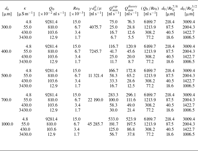
 $Q_{\textit{min}}\sim \gamma d^2_n/\mu$
. Although the scaling law approximately captures the power law dependence on the needle diameter, it overestimates the minimum flow rate by two to three orders of magnitude when compared with the measured values of
 $Q_{\textit{min}}$
reported in the same work.
Furthermore, in their cone-jetting experiments with viscous liquids, the range of electrical conductivity
 $\kappa$
, considered by Scheideler & Chen (Reference Scheideler and Chen2014), was limited to
 $\mathcal{O}(10^2{-}10^4\,\unicode {x03BC}$
S m−1). Consequently, their experiments did not capture the dependence of
 $Q_{\textit{min}}$
on
 $\kappa$
, resulting in an incorrect scaling law for the minimum flow rate, which is independent of the electrical conductivity of the viscous liquid. These contrasting findings have resulted in two groups of thought regarding the minimum flow rate of liquids satisfying the
 $\beta {\textit{Re}_0}\lt 1$
criterion. One of them suggests that
 $Q_{\textit{min}}$
depends only on the physical properties of the liquid, including
 $\kappa$
, and is independent of the geometrical parameters such as
 $d_n$
. The other argues that
 $Q_{\textit{min}}$
is independent of
 $\kappa$
but strongly depends on
 $d_n$
, specifically
 $Q_{\textit{min}} \sim d^2_n$
.
Therefore, based on the previous discussion, we conclude that the minimum flow rate of cone-jets of liquids with
 ${\beta \mathrm{Re}}_0 \lt 1$
is still not fully understood. Consequently, an extensive investigation is required across a wide range of needle diameters and electrical conductivity to understand the parameters that influence the minimum flow rate. Moreover, the current literature also lacks experimentally validated scaling laws for the minimum flow rate and the associated quantities, such as the jet diameter at the minimum flow rate.
1.1. Scope of the present work
In this work, we present theoretical scaling laws for the minimum flow rate of the Taylor cone-jet and the jet diameter at the minimum flow rate of highly viscous liquids, along with their experimental validation. For the minimum flow rate experiments, we employ highly viscous liquids with electrical conductivity spanning over four orders of magnitude and stainless steel needles with a blunt end. Specifically, we show that the minimum flow rate scales as
 $Q_{\textit{min}}\sim Q_0 (d_n/d_0 )^{8/5} {{\textit{Re}_0}}^{7/5}$
and the jet diameter at the minimum flow rate scales as
 $d\sim d_0 (d_n/d_0 )^{3/5} {{\textit{Re}_0}}^{2/5}$
. These scaling relations show excellent agreement with the experimental data for viscous liquids with electrical conductivity varying over four orders of magnitude. In addition, we present the limits of the regime in which these scaling laws are valid.
We begin by presenting the details of the experimental set-up, methodology and the data in § 2. Section 3 presents dimensional analysis and empirical correlations for the minimum flow rate, and the jet diameter at the minimum flow rate. Section 4 presents the theoretical scaling analysis and validation of the derived scaling relations with our experimental data and that obtained from the literature. In § 5, we discuss the validity of the assumptions based on which the scaling laws were derived. Subsequently, we discuss the limiting conditions under which the minimum flow rate of highly viscous liquid follows the derived scaling laws and shows dependence on the needle diameter. Lastly, § 6 provides the concluding remarks.
2. Experiments and results
In this section, we present the experimental methodology and the measurements to estimate the minimum flow rate for steady cone-jetting. We also present the measurements of the jet diameter and the total current carried by the jet at the minimum flow rate condition.
2.1. Experimental set-up
Figure 2 shows the schematic of the experimental set-up used for steady cone-jetting experiments. To measure the minimum flow rate, we employed a needle-plate configuration, wherein the needle was mounted on a vertical translation stage and a fine wire-mesh collector was positioned below the needle at a controllable distance (
 $H$
) from the needle tip, as shown in figure 2. A high-precision syringe pump (KD Scientific Legato 100, USA) was used to feed a viscous liquid with the desired flow rate
 $Q$
to a needle with an outer diameter
 $d_n$
. A DC high-voltage power supply (Keithley-2290-10, USA) was used to apply a potential difference
 $V$
between a needle and the collector. The current
 $I$
carried by the cone-jet was measured using a custom-built ammeter with precision operational amplifiers (op-amps). The total current carried by the cone-jet was directed to the inverting terminal of the op-amp (OPA227P, Texas Instruments), while the voltage drop across a 10 M
 $\varOmega$
shunt resistor was monitored and measured using a multimeter (Hewlett Packard 34401a, precision of 10
 $^{-6}$
mV). Subsequently, the total current carried by the jet was calculated as
 $I=V_{\textit{sh}}/R_{\textit{sh}}$
, where
 $R_{\textit{sh}}$
is the resistance of the shunt resistor and
 $V_{\textit{sh}}$
is the measured voltage drop across the shunt resistor. To ensure high accuracy in the current measurement, the non-inverting terminal of the op-amp was grounded through another precision op-amp (MCP-601, Texas Instruments). To visualise and capture the steady-state images of the cone-jet, a stereo-zoom microscope (Radical Scientific,
 $0.8-4.5\times$
zoom), equipped with a CMOS camera (Radical Scientific, Procam HS
 $-$
5) and a collimated LED light source (Thorlabs, USA), was employed. To measure the asymptotic jet diameter, images of a segment of the jet were captured at a distance of
 $0.5H$
from the needle tip using a separate CMOS camera (Basler acA640–750 um) equipped with a zoom lens (
 $0.7-4.5\times$
zoom). The raw images were processed to remove the background in MATLAB.
Schematic representation of the experimental set-up employed for steady cone-jetting of viscous leaky dielectric liquids. A stainless steel needle with an outer diameter
 $d_n$
and a blunt end is fixed at a distance
 $H$
from the collector. The highly viscous liquid is fed to the stainless steel needle at a flow rate of
 $Q$
, and a potential difference of
 $V$
is maintained between the needle tip and the collector. Due to the application of a strong electric field
 $\mathcal{O}(10^{6}\,\mathrm{V\,m^{- 1}})$
, the meniscus of the liquid gets stretched and a fine jet issues from the cone tip. Simultaneously, the jet is visualised through a horizontally mounted microscope, and images of the jet are captured using a CMOS camera for further analysis. An ammeter, connected between the collector and the ground, measures the total current carried by the jet. The snapshot shows a steady cone-jet of pure glycerol issuing out from a stainless steel needle with an outer diameter of
 $d_n$
= 500
 $\unicode {x03BC}$
m at a flow rate of
 $Q=10\,\unicode {x03BC}$
l min−1, while a potential difference of
 $V=3.4\,$
kV is maintained across a gap of
 $H=5\,$
mm between the needle and the collector.

2.2. Materials and experimental procedure
To quantify the dependence of the minimum flow rate on the needle diameter, we employed five stainless steel needles, each having a flat end and a length of 25 mm, with outer diameters of
 $d_n=300, 400, 500, 700$
and
 $1000\,\unicode {x03BC}$
m. To observe the effect of the stand-off distance on the minimum flow rate of each liquid, we varied
 $H$
between 3 and 18 mm. For minimum flow rate experiments, we used pure glycerol (Sigma Aldrich) and glycerol doped with varying concentrations of sodium chloride (CDH, India) to achieve a wide range of electrical conductivity spanning four orders of magnitude. Note that the liquids used in the experiments wet the stainless steel surface and, hence, the meniscus is pinned at the outer edge of the needle as shown in figure 2. The electrical conductivities of the doped glycerol solutions were measured using a conductivity meter (Jenway 4510, UK) immediately after the measurement of
 $Q_{\textit{min}}$
. The densities
 $\rho$
of the liquids were measured by weighing a known volume (10 ml) of each solution using a precision weighing balance (A&D Weighing, FZ
 $-$
300 GD, precision of 1 mg). The interfacial tension
 $\gamma$
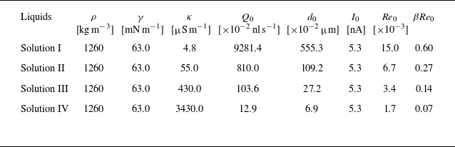
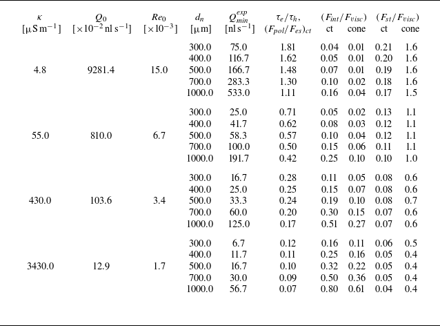
of the liquid–air interface was measured using the pendant drop method. Table 1 provides the measured properties of the liquids and reference scales for flow rate, jet diameter and total current denoted as
 $Q_0= \gamma \varepsilon _0/(\rho \kappa )$
,
 $d_0= [\gamma \varepsilon _0^2/ (\rho \kappa ^2 ) ]^{1/3}$
and
 $I_0 =\sqrt {\gamma ^2 \varepsilon _0/\rho }$
(Gañán-Calvo et al. Reference Gañán-Calvo, Lasheras, Dávila and Barrero1994), respectively, and the corresponding values of
 ${\textit{Re}}_0=\rho Q_0/ (\mu d_0 )$
; a detailed discussion on these reference scales is provided in § 3. The values of other relevant physical properties, such as dynamic viscosity (
 $\mu$
) and dielectric constant (
 $\beta$
), were considered to be the same as those of pure glycerol and were obtained from the literature (Scheideler & Chen Reference Scheideler and Chen2014) as
 $\mu =1.4$
Pa s and
 $\beta =41$
, respectively. For each solution, a fresh 5 ml syringe, a tubing and five needles were used to avoid contamination. Before commencing the experiment, the entire system was thoroughly flushed with the working solution to remove any trapped air bubbles.
Values of density (
 $\rho$
), interfacial tension (
 $\gamma$
) and electrical conductivity (
 $\kappa$
) of the working liquids measured at
 $20\,^\circ \textrm {C}$
. Also tabulated are the reference scales for flow rate (
 $Q_0$
), jet diameter (
 $d_0$
) and the total current carried by jet (
 $I_0$
), along with the corresponding values of the electrohydrodynamic Reynolds number (
 ${\textit{Re}_0}$
) and
 $\beta {\textit{Re}_0}$
. The Ohnesorge number, defined as
 $\textit{Oh}=\mu /\sqrt {\rho \gamma d_n}$
for solutions I
 $-$
IV are in the range of
 $5.0-9.1$
corresponding to the needle diameters employed in the present study, which vary between
 $300\;\mathrm{and}\;1000\,\unicode {x03BC}$
m.

To determine the minimum flow rate for a specific solution, we performed experiments for a large number of
 $(V, Q)$
combinations. We chose flow rates specifically around the
 $Q_0$
value, such that steady cone-jetting of the liquid was possible. Out of these large
 $(V, Q)$
data sets, the smallest flow rate at which steady jetting could be observed was considered the minimum flow rate and the corresponding value of the applied potential was considered the threshold potential. Each experiment was repeated five times to ascertain the repeatability of the experiments. The minimum flow rate values reported here are the mean values for the corresponding operating conditions. Similarly, the reported values of the total current carried by the jet and the jet diameter at the minimum flow rate are also the mean values for the corresponding operating conditions. The random uncertainties in the measurement of the minimum flow rate and the total current carried by the steady jet were estimated using
 $t$
-distribution (Bahga Reference Bahga2021). The total uncertainties in the measurement of the minimum flow rate and the total current were dominated by random uncertainty, which were less than
 $5\,\%$
at a
 $95\,\%$
confidence level. However, the total uncertainty in the measurement of the jet diameter was the result of the random uncertainty, estimated using
 $t$
-distribution and systematic uncertainty, influenced by the effective pixel size of the camera sensor (
 $1\,\unicode {x03BC}$
m). The total uncertainty in diameter measurements, obtained by combining systematic and random uncertainties, was less than
 $5\,\%$
of the mean jet diameter at a
 $95\,\%$
confidence level. Note that all experiments were performed at an ambient temperature range of
 $20\,^\circ \textrm {C}$
–
 $ 22\,^\circ \textrm {C}$
and a relative humidity range of
 $30\,\%{-}40\,\%$
.
2.3. Experimental results and discussion
2.3.1. Measurements of minimum flow rate of viscous liquids
In this section, we present the experimental data for pure glycerol (Solution I) and salt-doped glycerol solutions (Solutions II
 $-$
IV) to elucidate the effect of stand-off distance, needle diameter and electrical conductivity of a viscous liquid on the minimum flow rate essential for steady cone-jetting.
To elucidate the effect of stand-off distance on the minimum flow rate, we performed experiments with solution I, varying
 $H$
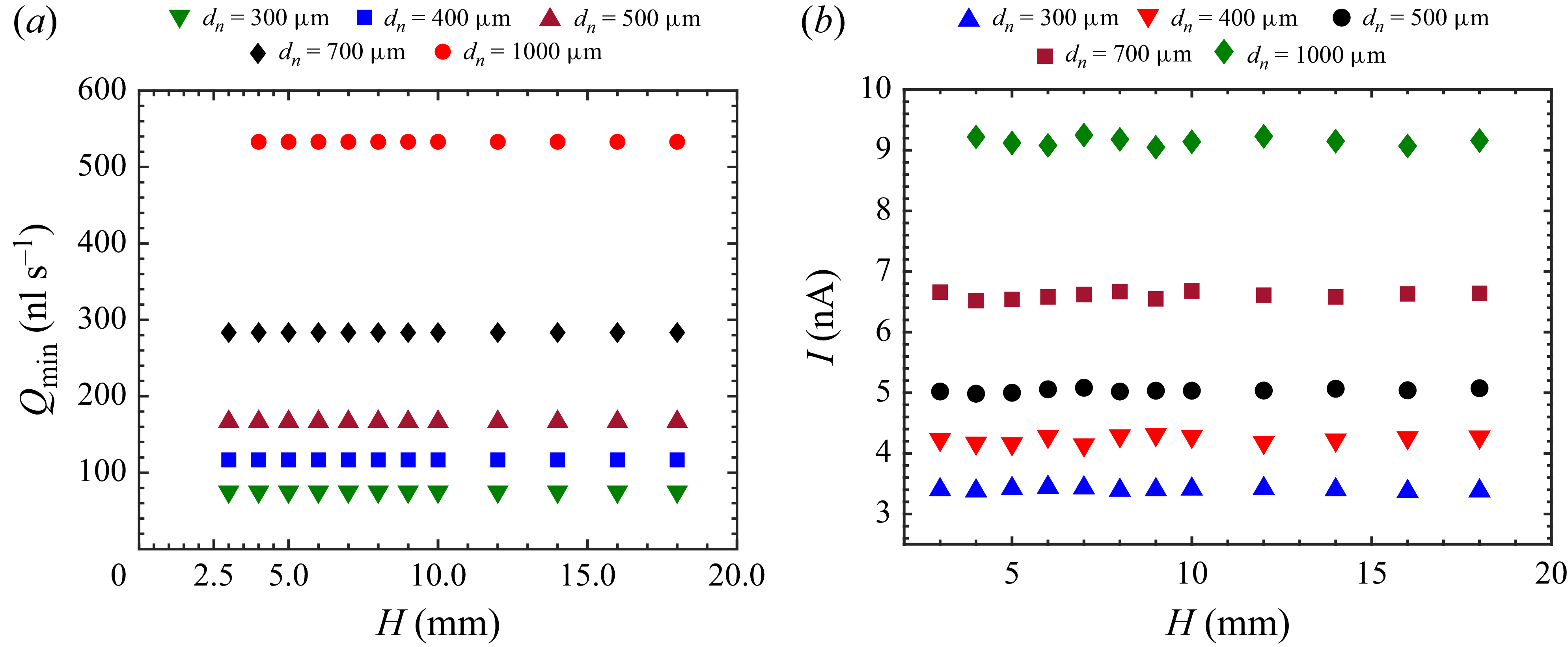
from 3 to 18 mm for a given needle. We then repeated the procedure for all the needles and measured the corresponding values of the minimum flow rate. Figure 3
 $(a)$
shows the variation of the minimum flow rate with the stand-off distance for all the needles. From figure 3
 $(a)$
, we note that
 $Q_{\textit{min}}$
is independent of the stand-off distance
 $H$
for a given needle diameter. However, the threshold potential corresponding to the minimum flow rate, that is, the minimum potential difference required for the onset of steady EHD-jetting, increases with increasing stand–off distance for all needle diameters. This trend suggests that, for a given needle diameter, the threshold electric field acting on the working liquid, near the needle tip, remains nearly the same for the range of
 $H$
considered in the present study. This observation is consistent with our earlier observation of
 $Q_{\textit{min}}$
being independent of
 $H$
. The exact dependence of the threshold potential on the geometrical parameters is discussed in detail in § 2.3.3.
Variation of (a) the minimum flow rate (
 $Q_{\textit{min}}$
) necessary for steady cone-jetting of solution I and (b) the total current carried by the jet at
 $Q_{\textit{min}}$
with the stand-off distance (
 $H$
). We infer that both minimum flow rate
 $Q_{\textit{min}}$
and the total current carried by the jet
 $I$
at
 $Q_{\textit{min}}$
are independent of stand-off distance
 $H$
.

However,
 $Q_{\textit{min}}$
monotonically increases with the needle diameter for all stand-off distances. For each case, we also measured the total current
 $I$
carried by the jet at the minimum flow rate condition. Figure 3
 $(b)$
shows the variation of
 $I$
with
 $H$
for solution I for all five needles. From figure 3
 $(b)$
, we note that the total current
 $I$
, similar to
 $Q_{\textit{min}}$
, is also independent of
 $H$
for a given needle diameter and increases with increasing needle diameter. Therefore, we can conclude that stand-off distance
 $H$
does not affect the minimum flow rate necessary for steady cone-jetting of a viscous liquid.
Next, to investigate the effect of the needle diameter and the electrical conductivity of the viscous liquids on the minimum flow rate essential for steady cone-jetting, we kept the stand-off distance fixed at
 $H=5\,$
mm. Figure 4(a–d) show images of the cone-jets corresponding to solutions I
 $-$
IV for
 $d_n=400\,\unicode {x03BC}$
m with minimum flow rate values of 116.7, 41.7, 25.0 and 11.7 nl s−1, respectively. From figure 4(a–d), we infer that the minimum flow rate and the corresponding jet diameter decrease with an increase in the electrical conductivity of the liquid for a fixed needle diameter. Figure 4(e–h) show the images of cone-jets corresponding to solutions I
 $-$
IV for
 $d_n=500\,\unicode {x03BC}$
m with minimum flow rate values of 166.7, 58.3, 33.3 and 16.7 nl s−1, respectively. Similar to steady jetting for a needle with
 $d_n = 400\,\unicode {x03BC}$
m, the minimum flow rate and the corresponding jet diameter decrease with an increase in the liquid conductivity for the needle with
 $d_n=500\,\unicode {x03BC}$
m.
Snapshots of steady Taylor cone-jets of solutions I–IV at the minimum flow rate condition. Steady state cone-jet images of solutions I–IV when flown through needles with outer diameters of
 $d_n=$
(a–d) 400 and (e–h) 500
 $\unicode {x03BC}$
m. The minimum flow rates of steady Taylor cone-jets for panels (a–d) and (e–h) are 116.7, 41.7, 25.0 and 11.7 nl s−1, and 166.7, 58.3, 33.3 and 16.7 nl s−1, respectively. From these observations, we infer that the minimum flow rate of Taylor cone-jets of highly viscous leaky dielectric liquid decreases with the increase in the electrical conductivity of the liquids for a particular needle and increases with the increase in the needle diameter for a given solution. Moreover, the jet diameter, similar to the minimum flow rate, decreases with the increases in the electrical conductivity of the liquid for a given needle diameter. and increases with the increase in the needle diameter for a given solution. For
 $(a-d)$
, the potential differences maintained between the needle tip and the collector necessary for steady cone-jetting are 3.3, 3.5, 3.7 and 3.8 kV, and 3.4, 3.7, 3.7 and 3.8 kV for panels
 $(e-h)$
, respectively. These potential differences, when changed slightly, resulted in pulsating jets in the respective experiments.

Next, to understand the effect of the needle diameter on the minimum flow rate of a viscous liquid, we refer to figure 3
 $(a)$
. Through figure 3
 $(a)$
, we have already shown that the minimum flow rate of solution I increases with the increase in the needle diameter for a given stand-off distance. To verify whether this trend holds for the other liquids, we compare the minimum flow rate values of steady cone-jetting across all the needle diameters while keeping the electrical conductivity fixed. We repeat this process for all four liquids. The comparison of figure 4(a–d) with figure 4(e–h) suggests that the minimum flow rate and the corresponding jet diameter increase with increasing needle diameter. Therefore, the increase in the minimum flow rate upon increasing
 $d_n$
is consistent for all four liquids, which have electrical conductivities spanning over four orders of magnitude.
To further explore the dependence of the minimum flow rate on the needle diameter, in figure 5
 $(a)$
, we plot the measured values of the minimum flow rate of all four liquids against the needle diameter on a logarithmic scale. The experimental data suggest that the minimum flow rate increases linearly with the needle diameter on a log–log plot, indicating a power-law variation of
 $Q_{\textit{min}}$
on
 $d_n$
with a positive exponent. Moreover, figure 5
 $(a)$
also indicates that for a given needle diameter, the minimum flow rate decreases with increasing electrical conductivity of the liquid.
Variation of the minimum flow rate (
 $Q_{\textit{min}}$
) in steady cone-jetting of highly viscous leaky dielectric liquids with the outer diameter of the needles (
 $d_n$
) and electrical conductivity of the liquids (
 $\kappa$
). (a) Variation of
 $Q_{\textit{min}}$
with
 $d_n$
on a log–log plot for solutions I
 $-$
IV. The experimental data of
 $Q_{\textit{min}}$
for each of the four liquids closely follow the scaling law
 $Q_{\textit{min}} \sim d^{1.7}_n$
. (b) Variation of
 $Q_{\textit{min}}$
with
 $\kappa$
of the four liquids used in the cone-jetting experiment for all the five needle diameters in a log–log plot. In this case, the same experimental data of
 $Q_{\textit{min}}$
aligns well with the scaling law
 $Q_{\textit{min}} \sim \kappa ^{-0.34}$
for each needle diameter.
 $(c)$
Minimum flow rate value predicted by the empirical correlation
 $Q^{\textit{corr}}_{\textit{min}}$
(2.1), which is in excellent agreement with the experimental data of the present work and that of Scheideler & Chen (Reference Scheideler and Chen2014).

To obtain the scaling of the minimum flow rate on the electrical conductivity of a solution, we plot the same data of
 $Q_{\textit{min}}$
in figure 5
 $(b)$
against the electrical conductivity of all four liquids on a logarithmic scale. We infer from the plot that the minimum flow rate decreases linearly with the conductivity of the liquid on a log–log plot, suggesting a power-law variation of
 $Q_{\textit{min}}$
on
 $\kappa$
but with a negative exponent.
Now that the dependence of the minimum flow rate on the needle diameter and the electrical conductivity of the liquid has been established, we perform a multi-variable regression analysis (Bahga Reference Bahga2021) with the experimental data of the present work to obtain the respective exponents, and subsequently the dimensional correlation for the minimum flow rate in terms of
 $d_n$
and
 $\kappa$
, given as
 \begin{align} Q^{\textit{corr}}_{\textit{min}} = 0.0075\,d_n^{1.7}\,\kappa ^{-0.34}. \end{align}
Note that
 $Q^{\textit{corr}}_{\textit{min}}$
,
 $d_n$
and
 $\kappa$
in (2.1) are in nl s−1,
 $\unicode {x03BC}$
m and
 $\unicode {x03BC}$
S m−1, respectively. The correlation, given by (2.1), suggests that the minimum flow rate scales as
 $Q_{\textit{min}} \sim d^{1.7}_n$
across liquids with varying electrical conductivities. This observation is consistent with the measurements of Scheideler & Chen (Reference Scheideler and Chen2014), who reported a scaling of the form
 $Q_{\textit{min}} \sim d^{1.45\pm 0.18}_n$
for salt-doped glycerol solutions. Moreover, the empirical correlation also suggests that
 $Q_{\textit{min}} \sim \kappa ^{-0.34}$
for all the needle diameters. We note that due to the weak dependence of the minimum flow rate on the electrical conductivity of the liquids, specifically
 $Q_{\textit{min}}\sim \kappa ^{-0.34}$
, Scheideler & Chen (Reference Scheideler and Chen2014), who performed cone-jetting experiments for a narrow range of electrical conductivity, incorrectly concluded that the minimum flow rate is independent of the electrical conductivity of the viscous liquid.
Next, we plot the minimum flow rate values predicted by the empirical correlation in the same plot where the experimental data are already overlayed, as shown in figures 5
 $(a)$
and 5
 $(b)$
. In these figures, the symbols represent the experimental data, whereas the dashed lines represent the predicted values of the minimum flow rate using the empirical correlation (2.1). To further establish the efficacy of the empirical correlation, in figure 5
 $(c)$
, we plot the minimum flow rate values obtained from the empirical correlation against the experimental data of both the present work and Scheideler & Chen (Reference Scheideler and Chen2014) on a logarithmic scale. From figure 5
 $(c)$
, we infer that the experimental data collapse on the dashed line, indicating a one-to-one correspondence.
Building on the present work, in § 2.3.2, we present the empirical scaling for the jet diameter at the minimum flow rate condition with
 $d_n$
and
 $\kappa$
. Subsequently, in § 2.3.3, we also present the scaling for the onset potential essential for steady cone-jetting at the minimum flow rate condition.
2.3.2. Jet diameter at the minimum flow rate
The jet diameter of a steady cone-jet is an important quantity for applications such as electrospraying and EHD-jet printing because it influences the size of the monodispersed droplets or the resolution of the deposited patterns. In the present study, we observe that cone-jets attain an asymptotic jet diameter far downstream of the cone-tip, within the precision of our measurements. This behaviour is consistent with the ballistic regime described by Gañán-Calvo (Reference Gañán-Calvo2025), which is particularly favourable for steady cone-jets of highly viscous liquids such as those used in the present study. Hereafter, the jet diameter refers to the asymptotic diameter measured downstream of the cone-tip.
Prior work on electrospraying and steady cone-jetting has shown that the jet diameter is positively correlated with the liquid flow rate. Moreover, from figure 4, we note that the jet diameter depends on the needle diameter and the electrical conductivity of the viscous liquid. In particular, the jet diameter decreases with increasing electrical conductivity and increases with the needle diameter for a given liquid. It is important to note that due to the high electrical conductivities of solutions III and IV, the corresponding jet diameters were below the resolution of the imaging system used in the present study. Consequently, the jet diameters for these two liquids could not be measured through imaging.
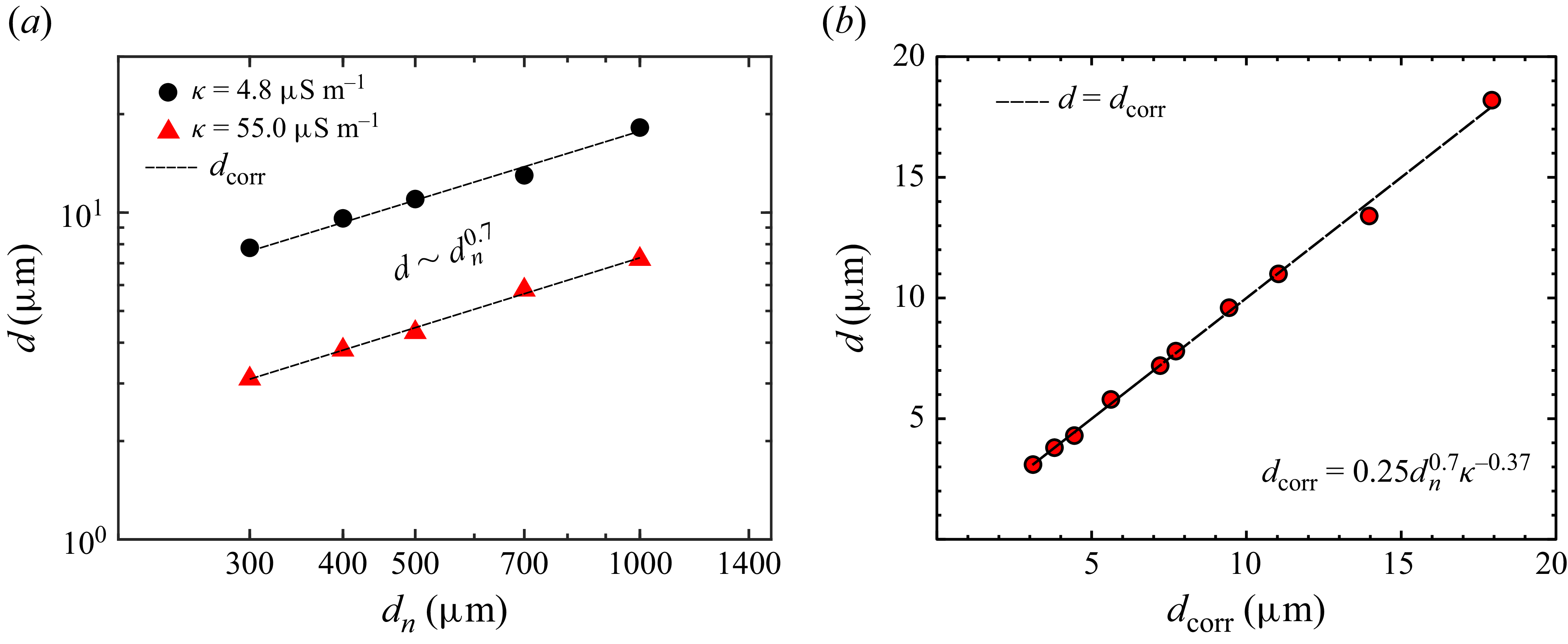
To explore the dependence of the jet diameter on the needle diameter, in figure 6
 $(a)$
, we plot the measured values of the jet diameter for solutions I and II against the outer diameter of the five needles employed in our experiments. The experimental data suggest that the jet diameter at the minimum flow rate increases monotonically with the needle diameter. From figure 6
 $(a)$
, we also note that the jet diameter at
 $Q_{\textit{min}}$
decreases with increasing electrical conductivity of the liquid. Therefore, the jet diameter exhibits a qualitatively similar dependence on the needle diameter and the electrical conductivity, as observed for the minimum flow rate. As a result, the jet diameter, similar to the minimum flow rate, can be represented as
 $d=c d^a_n \kappa ^b$
, where
 $a$
,
 $b$
and
 $c$
are constants to be determined using multivariable regression analysis (Bahga Reference Bahga2021). The resulting empirical correlation for the jet diameter is given by
 \begin{align} d_{\textit{corr}} = 0.25 d^{0.7}_n \kappa ^{-0.37}. \end{align}
Here,
 $d_{\textit{corr}}$
,
 $d_n$
and
 $\kappa$
are in
 $\unicode {x03BC}$
m and
 $\unicode {x03BC}$
S m−1, respectively. Although the dimensional correlation (2.2) is based on the jet diameter data of two liquids (Solutions I and II) only, we will justify the applicability of the correlation in §§ 4.4 and 4.5 using theoretical scaling analysis.
(a) Variation of the jet diameter
 $d$
at the minimum flow rate condition with the outer diameter of the needles (
 $d_n$
) for solutions I and II.
 $(b)$
Jet diameter predicted by the proposed correlation
 $d_{\textit{corr}}$
(2.2), which aligns well with the experimental observation.

Moreover, the experimentally measured jet diameter, when plotted against the predicted values in figure 6
 $(b)$
, collapses on the
 $45^\circ$
line indicating a one-to-one correspondence. Therefore, from figures 6
 $(a)$
and 6
 $(b)$
, we infer that the empirical correlation given by (2.2) provides an excellent prediction of the jet diameter.
2.3.3. Onset potential at the minimum flow rate
To ensure steady cone-jetting at the minimum flow rate condition, the applied potential has to be equal to the critical value known as the onset potential
 $V_{\textit{onset}}$
. At
 $V_{\textit{onset}}$
, flow rates at and above
 $Q_{\textit{min}}$
provide steady cone-jetting, whereas flow rates below
 $Q_{\textit{min}}$
result in a pulsating cone-jet (Bober & Chen Reference Bober and Chen2011; Chen Reference Chen2011 ). Thus, for a given solution and geometrical configuration, the minimum flow rate alone has significance only if reported along with
 $V_{\textit{onset}}$
(Bober & Chen Reference Bober and Chen2011; Chen Reference Chen2011). A good initial approximation of
 $V_{\textit{onset}}$
is therefore essential for locating
 $Q_{\textit{min}}$
of steady cone-jetting of a solution. In § 2.3.1, we present the experiments with solution I to show that
 $Q_{\textit{min}}$
is independent of
 $H$
. For the same set of experiments, we also recorded the onset potential at which steady cone-jetting was obtained. Figure 7
 $(a)$
shows the variation of onset potential
 $V_{\textit{onset}}$
with varying needle-to-collector distance
 $H$
for all five needles that are employed in the present work for solution I. This figure shows that
 $V_{\textit{onset}}$
monotonically increases with increasing
 $H$
for a given value of
 $d_n$
and also increases with the increasing
 $d_n$
for a given
 $H$
. To further elucidate the dependence of
 $V_{{{onset}}}$
on
 $H$
and
 $d_n$
, we scale the data represented in figure 7
 $(a)$
with the reference potential
 $V_{{ref}} =(\gamma d_n/\varepsilon _0)^{1/2}$
(Zeleny Reference Zeleny1935) and plot against the aspect ratio
 $\chi =(H/d_n)$
in a semi-log plot, as shown in figure 7
 $(b)$
. From figure 7
 $(b)$
, we observe that all the data points collapse to a single curve showing that the dimensionless onset potential
 $\tilde {V}_{\textit{onset}}=(V_{\textit{onset}}/V_{{ref}})$
varies logarithmically with the aspect ratio
 $\chi$
.
(a) Variation of the onset potential essential for steady cone-jetting at the minimum flow rate (
 $Q_{\textit{min}}$
) condition with the geometrical parameters of a cone-jetting set-up such as
 $H$
and
 $d_n$
for solution I.
 $(b)$
Linear variation of dimensionless onset potential
 $\tilde {V}_{\textit{onset}}$
with
 $4\chi$
on a semi-log plot, which suggests a logarithmic dependence.

The logarithmic dependence of
 $\tilde {V}_{\textit{onset}}$
on
 $\chi$
can be established by deriving the relationship for the electric field at the needle tip,
 $E=E(V_{\textit{onset}},d_n, H)$
. From the perspective of electric field distribution, the needle tip and the protruding liquid meniscus jointly can be approximated as a point electrode facing a flat counter electrode. The corresponding electric field at the tip of a needle for a point-plane geometry can be expressed as (Loeb et al. Reference Loeb, Kip, Hudson and Bennett1941; Smith Reference Smith1986),
 \begin{equation} E\sim \frac {V_{\textit{onset}}}{d_n\ln (4\chi )}. \end{equation}
Next, the potential required to set in the cone-jet mode at the minimum flow rate condition can be approximated by substituting the electric field
 $E$
in (2.3) with Taylor’s electrostatic field,
 $E\sim (\gamma /(\varepsilon _0 d_n) )^{1/2}$
(Taylor Reference Taylor1964). Upon substitution, we get
 \begin{align} \frac {V_{\textit{onset}}}{d_n\ln (4\chi )} \sim \left (\frac {\gamma } {\varepsilon _0 d_n}\right )^{1/2}, \end{align}
which shows that
 \begin{align} \tilde {V}_{\textit{onset}} \sim \ln (4\chi ). \end{align}
Hence, for a given liquid,
 $\tilde {V}_{\textit{onset}}$
varies logarithmically with
 $\chi$
and for a given geometrical configuration,
 $V_{\textit{onset}}$
depends only on the interfacial tension of the liquid. From figure 7
 $(b)$
, we also note that the slope of the line that shows a logarithmic dependence of
 $\tilde {V}_{\textit{onset}}$
on
 $\chi$
has a value of 0.5, which is in agreement with the findings of the previous studies (Loeb et al. Reference Loeb, Kip, Hudson and Bennett1941; Smith Reference Smith1986; Gañán-Calvo et al. Reference Gañán-Calvo, Lasheras, Dávila and Barrero1994; Pantano et al. Reference Pantano, Gañán-Calvo and Barrero1994). Therefore, we can rewrite (2.5) as
 \begin{align} \tilde {V}_{\textit{onset}}=0.5 \ln (4\chi ). \end{align}
Thus, (2.6) provides an estimate of the onset potential required to establish steady cone-jetting of highly viscous liquids for a given geometrical configuration at the minimum flow rate condition, and will be useful in applications such as EHD-jet printing, electrospinning and electrospraying while operating at or near
 $Q_{\textit{min}}$
.
3. Dimensional analysis and empirical correlation
We here present a dimensional analysis to describe the relevant dimensionless groups that influence the minimum flow rate necessary for steady cone-jetting of a highly viscous liquid. Thereafter, we reformulate the empirical correlations for the minimum flow rate and the jet diameter in terms of the identified dimensionless groups. Although, the dimensional empirical correlations for
 $Q_{\textit{min}}$
and
 $d$
in terms of the needle diameter (
 $d_n$
) and the electrical conductivity (
 $\kappa$
) of the liquid have been proposed in §§ 2.3.1 and 2.3.2, their validity is limited to salt-doped glycerol solutions only. Therefore, empirical correlations in the dimensionless form are necessary to extend their applicability to steady cone-jetting of any Newtonian highly viscous liquid.
The dimensional quantities that essentially govern the steady cone-jetting can be grouped into the following three categories.
-
(i) The operating parameters, such as the flow rate of the viscous liquid
 $Q$
and the potential difference maintained between the needle tip and the collector
$V$
.
-
(ii) The geometrical parameters, such as the outer diameter of the needle
$d_n$
, and the distance between the needle tip and the collector
$H$
. -
(iii) The physical properties of the liquid, such as density
$\rho$
, dynamic viscosity
$\mu$
, electrical conductivity
$\kappa$
, interfacial tension
$\gamma$
and electrical permittivity of the liquid
$\varepsilon _i$
, and the properties of the surrounding medium (Gañán-Calvo Reference Gañán-Calvo2004; Singh et al. Reference Singh, Srivastava and Bahga2022).


Typically, the surrounding medium is quiescent air, which allows one to exclude its dynamical effects on the system, and the only important parameter characterising its influence is the electrical permittivity
 $\varepsilon _0=8.854\times {10}^{-12}$
Fm
 $^{-1}$
. However, the applied potential
 $V$
is excluded from the dimensional analysis because, for a given solution, needle diameter and stand-off distance, the minimum flow rate of steady cone-jetting can be realised for a unique value of the applied potential,
 $V_{\textit{onset}}$
. Therefore, the applied voltage is not considered as an independent variable and is excluded from the list of parameters that influence
 $Q_{\textit{min}}$
(Bober & Chen Reference Bober and Chen2011).
In the steady cone-jet mode, the conduction current dominates in the cone region near the tip of the needle, where the flow speed and the surface charge density on the liquid–air interface are low. However, the surface convection current dominates in the jet segment, where the conduction resistance is too high due to the small values of the jet diameter (Higuera Reference Higuera2003). In the intermediate region, which connects the cone and the fine jet, the conduction and surface convection currents are of the same order of magnitude (Gañán-Calvo Reference Gañán-Calvo1997b
, Reference Gañán-Calvo1999; Gañán-Calvo et al. Reference Gañán-Calvo, Rebollo-Muñoz and Montanero2013). Gañán-Calvo (Reference Gañán-Calvo1997b
) showed that in the steady cone-jet mode, the jet emission for leaky dielectric liquids relies on the balance of forces in this intermediate region. This intermediate region is termed as the current transfer region and the characteristic size of this region is much smaller than that of the cone-jetting set-up (Gañán-Calvo et al. Reference Gañán-Calvo, Rebollo-Muñoz and Montanero2013). Accordingly, Gañán-Calvo et al. (Reference Gañán-Calvo, Rebollo-Muñoz and Montanero2013) excluded geometrical parameters such as stand-off distance
 $H$
and needle diameter
 $d_n$
from the list of parameters affecting
 $Q_{\textit{min}}$
. We have also shown through figure 3
 $(a)$
that the minimum flow rate of steady cone-jetting of a viscous liquid is independent of the stand-off distance
 $H$
. Therefore, we do not consider
 $H$
to influence the minimum flow rate. However, our experimental observation indicates that the minimum flow rate of a viscous liquid in steady cone-jetting does depend on the needle diameter
 $d_n$
. In particular, we observed a dependence of the form
 $Q_{\textit{min}} \sim d_n^{1.7}$
, as shown in figure 5
 $(a)$
. Thus, the minimum flow rate
 $Q_{\textit{min}}$
ejected in the steady cone-jet mode can be represented as a function of seven dimensional parameters as
 \begin{align} Q_{\textit{min}}=F\left (\rho ,\gamma ,\mu ,\kappa ,d_n,\varepsilon _i,\varepsilon _0\right )\!. \end{align}
Using the Buckingham
 $\varPi $
theorem (Evans Reference Evans1972), we can group the dimensional quantities into four independent dimensionless groups as
 \begin{align} \tilde {Q}_{\textit{min}}=\dfrac {Q_{\textit{min}}}{Q_0},\quad \tilde {d_n}=\dfrac {d_n}{d_0},\quad {\textit{Re}}_0=\dfrac {\rho Q_0}{\mu d_0}=\left (\dfrac {\gamma ^2 \varepsilon _0 \rho }{\mu ^3 \kappa }\right )^{1/3}\quad \mathrm{and}\quad \beta = \dfrac {\varepsilon _i}{\varepsilon _0}. \end{align}
Here,
 $Q_0$
and
 $d_0$
are defined by
 \begin{align} Q_0=\dfrac {\gamma \varepsilon _0}{\rho \kappa } \quad \mathrm{and}\quad d_0=\left (\dfrac {\gamma \varepsilon _0^2}{\rho \kappa ^2}\right )^{1/3} \!. \end{align}
The reference scales for the flow rate
 $Q_0$
and the jet diameter
 $d_0$
in the current transfer region, defined by (3.3a
) and (3.3b
), respectively, can be obtained by order-of-magnitude analysis, as shown by Higuera (Reference Higuera2003). Briefly, the balance between the inertia and the surface tension forces in the inertia-dominated jetting results in the departure of the surface from the steady Taylor cone. Mathematically, an order-of-magnitude balance between the two forces yields
 $\rho Q_0^2/d_0^4 = \gamma /d_0$
, which, on further simplification, leads to the expression
 $d_0 =(\rho Q_0^2/\gamma )^{1/3}$
. This expression is the inertial scale for the jet diameter, provided by Fernandez De La Mora et al. (Reference Fernandez De La Mora, Navascues, Fernandez and Rosell-Llompart1990). Similarly, the balance between the surface tension force (
 $\gamma /d_0$
) and the force due to normal electric stress (
 $\varepsilon _0 E_0^2$
) gives the scale of the electric field as
 $E_0= \sqrt {\gamma /(\varepsilon _0 d_0)}$
. Subsequently, the scales for the electric potential and the charge density are obtained as
 $V_0 = E_0 d_0 =\sqrt {\gamma d_0/\varepsilon _0}$
and
 $\sigma _0=\varepsilon _0 E_0$
. Next, the balance between the bulk conduction
 $(I_b=\kappa d_0^2 E_0 )$
and surface convection current
 $(I_s= \sigma _0 Q_0 d_0/d_0^2= \varepsilon _0 E_0 Q_0/d_0)$
at the current transfer region yields
 $d_0 = (\varepsilon _0 Q_0/\kappa )^{1/3}$
. Finally, we equate the two expressions of
 $d_0$
,
 $d_0 = (\rho Q^2_0/\gamma )^{1/3}$
and
 $d_0 = (\varepsilon _0 Q_0/\kappa )^{1/3}$
, to get the reference scales for flow rate (
 $Q_0$
) and jet diameter (
 $d_0$
) in terms of the physical properties of the liquids, as given by (3.3a
) and (3.3b
), respectively. For liquids with low to moderate electrical permittivity (
 $\beta$
), the dependence of minimum flow rate on electrical permittivity can be neglected (Scheideler & Chen Reference Scheideler and Chen2014). Therefore, we can express the relationship between the dimensionless groups in (3.2) as
 \begin{align} \tilde {Q}_{\textit{min}} = G\big (\tilde {d_n}, {{\textit{Re}_0}}\big ). \end{align}
The functional dependence of
 $\tilde {Q}_{\textit{min}}$
on
 $\tilde {d_n}$
and
 ${\textit{Re}_0}$
described in (3.4) can be obtained empirically or by mathematical modelling. To obtain a dimensionless empirical correlation for the minimum flow rate, we use the dimensional empirical correlation (2.1) and subsequently substitute
 $d_n =\tilde {d_n} d_0$
and
 $\kappa = \gamma ^2 \varepsilon _0 \rho /({\textit{Re}_0}^3 \mu ^3)$
from (3.2). The substitution yields
 \begin{align} \tilde {Q}_{\textit{min}} Q_0 &= 0.0075 \big (\tilde {d_n} d_0\big )^{1.7} \left (\dfrac {\gamma ^2 \varepsilon _0 \rho }{{\textit{Re}_0}^3 \mu ^3}\right )^{-0.34}, \notag \\ \tilde {Q}_{\textit{min}} &=0.3\,\tilde {d_n}^{1.7}{{\textit{Re}_0}}^{1.4}. \end{align}
Similar to
 $\tilde {Q}_{\textit{min}}$
, the dimensionless jet diameter
 $\tilde {d}=d/d_0$
at the minimum flow rate condition can also be expressed as a function of
 $\tilde {d_n}$
and
 ${\textit{Re}_0}$
. We write
 \begin{align} \tilde {d} = G^{\prime }\big (\tilde {d_n}, {{\textit{Re}_0}}\big ). \end{align}
Next, to get a dimensionless empirical correlation for the jet diameter at the minimum flow rate condition, we substitute
 $d_n =\tilde {d_n}d_0$
and
 $\kappa = \gamma ^2 \varepsilon _0 \rho /({\textit{Re}_0}^3 \mu ^3)$
obtained from (3.2) into the dimensional empirical correlation for the jet diameter, given by (2.2). The substitution yields
 \begin{align} \tilde {d} d_0 &= 0.25 \big (\tilde {d_n}d_0\big )^{0.7} \left (\dfrac {\gamma ^2 \varepsilon _0 \rho }{{\textit{Re}_0}^3 \mu ^3}\right )^{-0.37}, \notag \\ \tilde {d} &=0.6\,\tilde {d_n}^{0.7}{{\textit{Re}_0}}^{0.5}. \end{align}
For a steady cone-jet, the inverse of electrohydrodynamic Reynolds number,
 ${\textit{Re}_0}^{-1}$
, signifies the relative importance of the viscous force with respect to the inertia and the interfacial tension forces, respectively, in the current transfer region. From table 1, we note that
 ${\textit{Re}_0}^{-1}$
calculated based on the reference scales of flow rate
 $Q_0$
and jet diameter
 $d_0$
indicates the dominance of viscous force over inertia and interfacial tension forces, respectively. Note that the inverse of the electrohydrodynamic Reynolds number denotes the electrohydrodynamic Ohnesorge number, defined as
 $\textit{Oh}_0=\mu /\sqrt {\rho \gamma d_0}$
(Nganguia et al. Reference Nganguia, Young, Layton, Lai and Hu2016). We also highlight that for the present study and that of Scheideler & Chen (Reference Scheideler and Chen2014),
 $Q_{\textit{min}}$
shows a dependence on
 $d_n$
even when
 $\tilde {d}_n \gtrsim 80$
. This is in contrast to the observation of Ponce-Torres et al. (Reference Ponce-Torres, Rebollo-Muñoz, Herrada, Gañán-Calvo and Montanero2018) since the liquids considered in the present study and that of Scheideler & Chen (Reference Scheideler and Chen2014) are highly viscous in nature.
Therefore, the proposed dimensionless empirical correlations, given by (3.5) and (3.7), successfully capture the importance of the viscous force, needle diameter and the electrical conductivity of the liquid. These correlations can now be employed to provide accurate estimates of the minimum flow rate and the corresponding jet diameters for steady cone-jetting of highly viscous Newtonian liquids.
Having established the dependence of the dimensionless minimum flow rate
 $\tilde {Q}_{\textit{min}}$
and the jet diameter
 $\tilde {d}$
on the dimensionless needle diameter
 $\tilde {d}_n$
and the electrohydrodynamic Reynolds number
 $\textit{Re}_0$
of the liquid, in the following sections, we try to provide a theoretical basis for the scaling behaviours observed for
 $\tilde {Q}_{\textit{min}}$
and
 $\tilde {d}$
. We also note that the empirical correlations suggest that with increasing value of
 $\tilde {d}_n$
, the minimum flow rate
 $\tilde {Q}_{\textit{min}}$
and corresponding jet diameter
 $\tilde {d}$
increase. However, these empirical correlations are valid within a bounded regime defined by lower and upper limits. In the subsequent theoretical analysis, specifically in § 5, we explicitly identify these bounds within which the empirical correlation for the minimum flow rate holds and beyond which the dependence of minimum flow rate on the needle diameter no longer applies.
4. Scaling analysis
4.1. Governing equations
In § 3, based on the experimental data and the dimensional analysis, we obtained the empirical correlations for the minimum flow rate and the corresponding jet diameter for Taylor cone-jetting of highly viscous liquids. However, to provide a physical reasoning underlying such a relationship, here, we derive similar scaling laws based on the governing equations describing steady cone-jets. To this end, we model a viscous liquid flowing through a metallic nozzle of outer diameter
 $d_n$
with a flow rate of
 $Q$
under the effect of the electric field
 $E$
due to the applied electric potential difference, as illustrated in figure 8. For the highly viscous liquids used in the present work, the Debye layer thickness,
 $\lambda _D$
, is significantly smaller than the jet diameter, with
 $\lambda _D \sim \mathcal{O}(0.1{-}1\,$
nm). In steady EHD-jets at the minimum flow rate condition, despite of a thin electric double layer, the effective charged region in the jet may still be large due to advection. Nevertheless, within the purview of the present study, we note that the dominant charged transport remains localised near the interface and the bulk may be treated effectively as electro-neutral. Accordingly, the leaky-dielectric model (Saville Reference Saville1997) provides a consistent reduced description of the force balances at the cone-tip and in the current transfer region. We note that outside this regime, the leaky-dielectric model may not hold and a fully coupled electrokinetic model may be required for solving the electrohydrodynamic jetting problem as discussed by López-Herrera et al. (Reference López-Herrera, Herrada and Gañán-Calvo2023). Therefore, to describe the steady cone-jetting of the viscous liquid, we assume the viscous liquid to behave as a leaky-dielectric (Saville Reference Saville1997).
Schematic representation of the Taylor cone-jet of a highly viscous liquid at the minimum flow rate configuration. The steady cone-jet can be divided into three regions, viz. the cone region, the fully developed jet region and the intermediate current transfer region, which connects the cone and the jet.

For a leaky-dielectric liquid, at the minimum flow rate condition, the residence time in the current transfer region is greater than or, at best, comparable to the charge relaxation time (Gañán-Calvo et al. Reference Gañán-Calvo, Rebollo-Muñoz and Montanero2013; Ponce-Torres et al. Reference Ponce-Torres, Rebollo-Muñoz, Herrada, Gañán-Calvo and Montanero2018). That is,
 $\tau _e/\tau _h \lesssim 1$
(Gañán-Calvo et al. Reference Gañán-Calvo, Rebollo-Muñoz and Montanero2013; Ponce-Torres et al. Reference Ponce-Torres, Rebollo-Muñoz, Herrada, Gañán-Calvo and Montanero2018), where
 $\tau _e =\beta \varepsilon _0/\kappa$
is the charge relaxation time scale and
 $\tau _h =Ld^2/Q$
is the convective time scale. Here,
 $d$
and
 $L$
denote the characteristic jet diameter and the length of the current transfer region, as illustrated in figure 8. The convective time scale can be considered as the residence time in the current transfer region. Thus, for a leaky-dielectric liquid, the condition for fast charge relaxation can be expressed as
 \begin{align} \dfrac {\tau _e}{\tau _h}= \dfrac {\beta \varepsilon _0 Q}{L d^2 \kappa } \lesssim 1. \end{align}
For a leaky-dielectric liquid satisfying (4.1), all the charges in the bulk of the liquid are quickly conducted to the liquid surface. Therefore, the free charge is present only on the jet surface, and there are no free charges present in the bulk solution and the surrounding medium. We note that the electric field,
 $E$
, inside and outside of the jet, satisfies (Saville Reference Saville1997)
 \begin{align} \boldsymbol{\nabla }\boldsymbol{\cdot }\boldsymbol{E}=0\quad \mathrm{and}\quad \boldsymbol{\nabla }\times \boldsymbol{E}=0. \end{align}
Because the electric field is irrotational, the tangential components of the electric field corresponding to the inner and the outer fluids at the surface of the jet are equal, hereafter denoted as
 $E_t$
. Moreover, following Gauss’s law, the normal components of the electric fields
 $(E_n^{\textit{out}}, E_n^{\textit{in}})$
at the jet surface can be related to the surface charge density
 $\sigma$
as
 $\sigma =\varepsilon _0 E_n^{\textit{out}}-\varepsilon _i E_n^{\textit{in}}$
.
For a leaky-dielectric liquid, we have
 $\varepsilon _i E_n^{\textit{in}} \ll \varepsilon _0 E_n^{\textit{out}}$
(Gañán-Calvo Reference Gañán-Calvo1997b
). Consequently, the expression for surface charge density reduces to
 $\sigma \approx \varepsilon _0 E_n^{\textit{out}}$
. For simplification, hereafter, we denote
 $E_n^{\textit{out}}$
as
 $E_n$
. Hence, the expression for surface charge density can be rewritten as
 $\sigma \approx \varepsilon _0 E_n$
. The interaction between the surface charge and the components of the electric field results in tangential (
 $\sigma E_t$
) and normal
 $ (\varepsilon _0 [{E_n}^2+ (\beta -1 ){E_t}^2 ] )$
electric stresses on the liquid surface. These electric stresses, along with the stresses due to interfacial tension force, viscous force and inertia, describe Taylor cone-jetting.
Considering rapid charge relaxation and radial momentum diffusion, the steady cone-jetting of a viscous leaky-dielectric liquid can be approximated as a quasi-one-dimensional (quasi-1-D) flow problem. The quasi-1-D governing equations (Feng Reference Feng2002) for mass and momentum conservation can be written respectively as
 \begin{align} Q = \pi R^2v \end{align}
and
 \begin{align} \dfrac {\mathrm{d}}{\mbox{d}z}\left (\dfrac {\rho v^2}{2}\right )=\rho g+\dfrac {3}{R^2}\dfrac {\mathrm{d}}{\mbox{d}z}\left (\mu R^2 \dfrac {\mbox{d}v}{\mbox{d}z}\right )+\dfrac {2\sigma E_t}{R}+\dfrac {\mathrm{d}}{\mbox{d}z}\left [\dfrac {\sigma ^2}{2\varepsilon _0}-\dfrac {\gamma }{R}+\dfrac {\varepsilon _0\left (\beta -1\right )E^2_t}{2}\right ]\!. \end{align}
We neglect the body force due to gravity in (4.4), as the Bond number
 ${Bo} =\rho g R^2/\gamma \ll 1$
. Next, we substitute
 $v=Q/{\pi R^2}$
from (4.3) and
 $\sigma \approx \varepsilon _0 E_n$
in (4.4) to get the modified momentum equation as (Gañán-Calvo Reference Gañán-Calvo2004),
 \begin{align} \underbrace {\dfrac {\mathrm{d}}{\mbox{d}z}\left (\dfrac {\gamma }{R}\right )}_{\text{I}}+\underbrace {\dfrac {\mathrm{d}}{\mbox{d}z}\left (\dfrac {1}{2\pi ^2}\dfrac {\rho Q^2}{R^4}\right )}_{\text{II}}+\underbrace {\dfrac {6\mu Q}{\pi R^2}{\dfrac {\mathrm{d}}{\mbox{d}z}}\left (\dfrac {1}{R}\dfrac {\mbox{d}R}{\mbox{d}z}\right )}_{\text{III}} = \underbrace {\dfrac {2\varepsilon _{o}E_{t}E_{n}}{R}}_{\text{IV}}+\underbrace {\dfrac {\mathrm{d}}{\mbox{d}z}\left [\dfrac {\varepsilon _{o} E^2_n}{2}\right ]}_{\text{V}}+\underbrace {\dfrac {\mathrm{d}}{\mbox{d}z}\left [\dfrac {\varepsilon _{o}\left (\beta -1\right )E_{t}^2}{2}\right ]}_{\text{VI}}\!. \end{align}
Here,
 $R$
,
 $v$
,
 $E_n$
and
 $E_t$
denote the radius of the jet at an axial location
 $z$
, the area-averaged axial velocity of the liquid, and the normal and tangential components of the local electric field acting on the liquid surface, respectively. The three terms on the left-hand side of (4.5), denoted as I, II and III, correspond to the axial components of the interfacial tension force, the liquid inertia and the viscous force per unit volume, respectively. Similarly, the three terms on the right-hand side of (4.5), denoted as IV, V and VI, represent the axial components of the tangential electrostatic surface force, and the electrostatic suction and polarization forces per unit volume, respectively. The terms on the left side of (4.5) restrict, while those on the right side of (4.5) drive the cone-to-jet transition (Gañán-Calvo Reference Gañán-Calvo2004).
In the presence of an external electric field, charges within the liquid migrate quickly to the liquid’s free surface, eventually modifying the local electric field. Historically, two contrasting models have been proposed to explain the dominant mechanism of charge transport. Melcher & Warren (Reference Melcher and Warren1971) proposed a model based on dominant bulk conduction, whereas Turnbull (Reference Turnbull2002) emphasised surface convection as the primary contributor. These two different views led to the distinct formulations of the current balance. Recognising the limitations of both the simplified approaches, Gañán-Calvo (Reference Gañán-Calvo1994) was the first to present a formulation that incorporates both conduction and convection contributions, as represented in (4.6). This modified formulation was further used by Gañán Calvo (Reference Gañán-Calvo1997a
) in the study of electrified jets. Therefore, the migration of charges to the free surface occurs through bulk conduction, followed by surface convection along the jet and the total current
 $I$
carried by the electrified jet consists of bulk conduction (
 $I_{\textit{cond}}$
) and the surface convection (
 $I_{\textit{con}v}$
) currents (Gañán-Calvo Reference Gañán-Calvo1994; Gañán Calvo Reference Gañán-Calvo1997a
; Ponce-Torres et al. Reference Ponce-Torres, Rebollo-Muñoz, Herrada, Gañán-Calvo and Montanero2018; Singh et al. Reference Singh, Srivastava and Bahga2022). Although the magnitudes of the conduction and surface convection currents vary along the axial direction, the total current
 $I$
, given by (4.6), remains constant throughout the length of the jet (Singh et al. Reference Singh, Choubey, Srivastava and Bahga2023). Therefore, the equation for conservation of charge at any axial location along the length of a steady cone-jet gives the total current
 $I$
, which can be expressed as
 \begin{align} I =\pi R^2 \kappa E_t +2\pi \sigma R v. \end{align}
The first and second terms on the right-hand side of (4.6) represent the conduction (
 $I_{\textit{cond}}$
) and the convection (
 $I_{\textit{con}v}$
) currents, respectively.
Now that we are equipped with the necessary governing equations that describe an electrified jet, we perform scaling analysis for the minimum flow rate required for steady cone-jetting of highly viscous leaky-dielectric liquid. At this point, it is pertinent to revisit the existing scaling laws for
 $Q_{\textit{min}}$
provided in the literature. This will help differentiate the jetting regimes for highly viscous liquids presented in this work from those documented in the literature. We note that in the subsequent discussions, specifically in §§ 4.2 and 4.4, the quasi-1-D model (4.5) has not been used for any quantitative estimation of the different force terms; rather, it is employed solely to identify the scaling of the different driving and resisting forces.
4.2. Existing scaling laws
In this section, we revisit the work of Gañán-Calvo et al. (Reference Gañán-Calvo, Rebollo-Muñoz and Montanero2013) and Scheideler & Chen (Reference Scheideler and Chen2014) before deriving the scaling laws for highly viscous liquids.
4.2.1. Insights from the work of Gañán-Calvo et al.
Gañán-Calvo et al. (Reference Gañán-Calvo, Rebollo-Muñoz and Montanero2013) assumed that the stability of the cone-jet mode at the minimum flow rate condition is primarily dependent on the local flow arising in the current transfer region. Furthermore, the characteristic length of the current transfer region is much smaller than those characterising the cone-jetting set-up, i.e.
 $L\ll d_n$
and
 $L\ll H$
. Because of the locality of the current transfer region, Gañán-Calvo
 $et\,al$
. reasoned that the stability of the cone-jet mode at the minimum flow rate condition does not depend on the length scales associated with the cone-jetting set-up.
Next, they suggested that, in the current transfer region, the balance of the primary supporting and resistant forces is essential to achieve and sustain a steady jet. Using
 $d$
and
 $L$
as the reference scales for the radial and axial lengths of the current transfer region, respectively, the axial momentum (4.5) suggests the scaling for all the resisting and the supporting forces in the current transfer region as follows.
-
(i) Resisting forces:
$\{\text{I}:\gamma d^{-1} L^{-1}, \text{II}:\rho Q^2 d^{-4}L^{-1}, \text{III}:\mu Q d^{-2}L^{-2}\}$
. -
(ii) Supporting forces:
$\{\text{IV}:\varepsilon _0 E_n E_t d^{-1}, \text{V}:\varepsilon _0 E_n^2 L^{-1}, \text{VI}:\varepsilon _0 \beta E_t^2 L^{-1}\}$
.


In particular, Gañán-Calvo et al. argued that in the current transfer region among the supporting forces, the polarisation force is, at best, comparable to the electrostatic suction force, whereas the tangential electric force is significantly smaller than the electrostatic suction force throughout the current transfer region. On the other hand, among the opposing forces, the viscous force is, at best, comparable to the inertia term and the interfacial tension force is negligibly small. Therefore, Ganan-Calvo et al. considered inertia and electrostatic suction forces to be the primary resisting and driving forces at the current transfer region. Subsequently, they derived the scaling relations for jet diameter and the length of the current transfer region as
 \begin{align} d \sim d_0 \left (\dfrac {Q}{Q_0}\right )^{1/2}\quad \mathrm{and}\quad L\sim d_0\left (\dfrac {Q}{Q_0}\right )\!, \end{align}
by considering the balance of these forces in the current transfer region.
Furthermore, Gañán-Calvo et al. (Reference Gañán-Calvo, Rebollo-Muñoz and Montanero2013) argued that at the minimum flow rate condition, there could be two scenarios for which steady jet emission is not possible.
-
(i) The viscous forces may become comparable with the inertia and resist the jet emission before the polarisation force, referred to as the viscous limit. In the viscous limit, the minimum flow rate and the jet diameter at the minimum flow rate scale as
(4.8a,b)respectively.
\begin{align} Q_{\textit{min}}\sim Q_0 {\textit{Re}_0}^{-1} \quad \mathrm{and}\quad d \sim d_0 {\textit{Re}_0}^{-1/2}, \end{align}
-
(ii) The polarisation force may become negative beyond the cone-jet transition region and oppose the driving force first, termed as the polar limit. In the polar limit, the minimum flow rate and the jet diameter at the minimum flow rate scale as
(4.9a,b)respectively.
\begin{align} Q_{\textit{min}}\sim Q_0 \beta \quad \mathrm{and}\quad d \sim d_0\beta ^{1/2}, \end{align}


From (4.8a
) and (4.9a
), Ganan-Calvo et al. noted that the ratio of the minimum flow rate for the viscous limit case to the minimum flow rate for the polar limit case equals to
 $\beta {\textit{Re}_0}$
. Therefore, they concluded that the term
 $\beta {\textit{Re}_0}$
dictates which limit out of the viscous and polar limits will govern the minimum flow rate of steady cone-jetting. In particular, for
 $\beta {\textit{Re}_0} \lt 1$
, the viscous limit governs
 $Q_{\textit{min}}$
and for
 $\beta {\textit{Re}_0} \gt 1$
, the polar limit governs
 $Q_{\textit{min}}$
.
To validate the proposed scaling laws, in their study, Ganan-Calvo et al. considered liquids that satisfy both
 $\beta {\textit{Re}_0}\lesssim 1$
and
 $\beta {\textit{Re}_0} \gt 1$
conditions. However, our focus here is exclusively on liquids that meet the
 $\beta {\textit{Re}_0}\lt 1$
criterion, which are tabulated in table 2. Among all liquids considered by Ganan-Calvo et al., 3-ethylene glycol, 4-ethylene glycol and 1-ethyl-3-methylimidazolium bis(trifluoromethylsulfonyl) imide (EMI-Im), which have electrical conductivities of
 $\mathcal{O}(10^{3}{-}10^{5}\,\unicode {x03BC}\rm {S\,m}^{-1})$
, satisfy the condition
 $\beta {\textit{Re}_0}\lt 1$
, as shown in table 2. Subsequently, to validate their scaling laws for the minimum flow rate, Ganan-Calvo et al. plotted the experimental data for the flow rate on a two-dimensional (2-D) regime plot, with
 $Q_{\textit{min}}/(\beta Q_0)$
along the ordinate and
 $(\beta {\textit{Re}_0})^{-1}$
on the abscissa, as shown in figure 9. In their case, for
 $\beta {\textit{Re}_0} \lt 1$
, the experimental data for the minimum flow rate lay just above the
 $(Q_{\textit{min}}/Q_0){\textit{Re}_0} =1$
line, validating the derived scaling law for the minimum flow rate,
 $Q_{\textit{min}}\sim Q_0 {\textit{Re}_0}^{-1}$
. Moreover, as we are dealing with the minimum flow rate, in figure 9, we only highlighted the lowest value of the flow rate that has been reported in figure 2 of Gañán-Calvo et al. (Reference Gañán-Calvo, Rebollo-Muñoz and Montanero2013).
Physical properties of the liquids used by Gañán-Calvo et al. (Reference Gañán-Calvo, Rebollo-Muñoz and Montanero2013) that satisfy the
 $\beta {\textit{Re}_0}\lt 1$
criterion. Also tabulated are the reference scales for the flow rate
 $Q_0$
and jet diameter
 $d_0$
, along with the corresponding values of the electrohydrodynamic Reynolds number
 ${\textit{Re}_0}$
,
 $\beta {\textit{Re}_0}$
and Ohnesorge number
 $(\textit{Oh})$
. The Ohnesorge number (
 $\textit{Oh}=\mu /\sqrt {\rho \gamma d_n}$
) reported in the table is evaluated based on the diameter of the needle,
 $d_n=100\,\unicode {x03BC}$
m, employed in the study of Gañán-Calvo et al. (Reference Gañán-Calvo, Rebollo-Muñoz and Montanero2013).

A two-dimensional regime plot for minimum flow rate of different liquids on a
 $Q_{\textit{min}}/(Q_0\beta )$
versus
 $1/(\beta {\textit{Re}_0})$
plot. The regime plot is divided into two regions
 $\beta {\textit{Re}_0}\lt 1$
and
 $\beta {\textit{Re}_0}\gt 1$
by the vertical boundary line (in blue colour),
 $\beta {\textit{Re}_0}=1$
. The region
 $\beta {\textit{Re}_0}\lt 1$
is further divided by the slanted boundary line (in red colour),
 $(Q_{\textit{min}}/Q_0){\textit{Re}_0} =1$
, into two sub-regions
 $(Q_{\textit{min}}/Q_0){\textit{Re}_0} \gt 1$
and
 $(Q_{\textit{min}}/Q_0){\textit{Re}_0} \lt 1$
. The minimum flow rate data from Scheideler & Chen (Reference Scheideler and Chen2014) and present work clearly fall within the unexplored
 $(Q_{\textit{min}}/Q_0){\textit{Re}_0} \lt 1$
region. The grey hollow circular symbols represent the minimum flow rate data gathered from literature (figure 2 of Gañán-Calvo et al. Reference Gañán-Calvo, Rebollo-Muñoz and Montanero2013), which fall in the
 $(Q_{\textit{min}}/Q_0){\textit{Re}_0} \gt 1$
region close to the boundary 2. The details of the plotted experimental data are provided in table 2, in table 4 and in table 6.

An alternative explanation of the minimum flow rate
 $Q_{\textit{min}} \sim Q_0 {\textit{Re}_0}^{-1}$
in the viscous limit can be given by considering the ratio of
 $\tau _{\mu }$
and
 $\tau _h$
. Here,
 $\tau _{\mu }$
represents the viscous diffusion time scale across the length of the current transfer region. Using (4.7), we show that
 \begin{align} \dfrac {\tau _{\mu }}{\tau _{h}}\sim \dfrac {\rho L^2 Q}{\mu L d^2} \sim \dfrac {Q_{\textit{min}} {\textit{Re}_0}}{Q_0} \gtrsim 1. \end{align}
Therefore,
 $(Q_{\textit{min}}/Q_0){\textit{Re}_0}\gtrsim 1$
is equivalent to stating that at the minimum flow rate condition, the viscous diffusion time scale,
 $\tau _{\mu } \sim \rho L^2/\mu$
, across the length of the current transfer region is greater than or comparable to the characteristic residence time scale,
 $\tau _h \sim Ld^2/Q$
.
Alternatively, the limit can be expressed in terms of the ratio of inertia force density (
 $F_{\textit{int}}$
, term
 $\text{II}$
of (4.5)) to the viscous force density (
 $F_{v\textit{isc}}$
, term
 $\text{III}$
of (4.5)) in the current transfer region. Using the respective scales of the force densities and (4.7), we get
 \begin{align} \left (\dfrac {F_{\textit{int}}}{F_{v\textit{isc}}}\right )\sim \dfrac {\rho Q^2 d^{-4} L^{-1}}{\mu Q d^{-2} L^{-2}} \sim \dfrac {\rho Q L}{\mu d^2}\sim \dfrac {Q_{\textit{min}} {\textit{Re}_0}}{Q_0} \gtrsim 1. \end{align}
Therefore, the assumption of Ganan-Calvo et al. that inertia is the dominant resisting force in the current transfer region is justified for the liquids listed in table 2.
Similarly, if we compare the electrostatic suction force density (
 $F_{\textit{es}}$
, term
 $\text{V}$
of (4.5)) with the polarisation force density (
 $F_{\textit{pol}}$
, term
 $\text{VI}$
of (4.5)) in the current transfer region, we note that
 \begin{equation} \left (\dfrac {F_{\textit{pol}}}{F_{\textit{es}}}\right )\sim \dfrac {\varepsilon _0 \beta E^2_t L}{L \varepsilon _0 E^2_n} \sim \dfrac {\beta E^2_t}{E^2_n} \sim \dfrac {\beta d^2}{L^2} \sim \dfrac {\beta Q_0}{Q}. \end{equation}
For the
 $\beta {\textit{Re}_0}\lt 1$
case, the minimum flow rate
 $Q_{\textit{min}} \sim Q_0 {\textit{Re}_0}^{-1}$
(see (4.8a
)) and
 $(F_{\textit{pol}}/F_{\textit{es}}) \sim \beta {\textit{Re}_0}\lt 1$
at the minimum flow rate condition. Therefore, the assumption of Ganan-Calvo et al. that at the minimum flow rate condition, in the current transfer region, the electrostatic suction force is the dominant driving force is justified for the liquids listed in table 2.
We note that the criteria
 $(Q_{\textit{min}}/Q_0){\textit{Re}_0} \gtrsim 1$
and
 $\beta {\textit{Re}_0}\lt 1$
can also be expressed as
 \begin{equation} \alpha _{\rho } \gtrsim \alpha ^{1/4}_{\mu }\quad \text{and}\quad \dfrac {\alpha _{\rho }}{\left (\beta -1\right )}\gt 1, \end{equation}
respectively, where
 $\alpha _{\rho }=Q_{\textit{min}}/Q_0$
and
 $\alpha _{\mu }= \alpha _{\rho }/{\textit{Re}_0}^3$
(Gañán-Calvo Reference Gañán-Calvo2004). These terms are widely used in the literature on Taylor cone-jets. We also note that (4.13) is the well-known criteria for the inertia electrostatic suction regime (IE regime) (Gañán-Calvo Reference Gañán-Calvo2004). Thus, the liquids considered by Gañán-Calvo et al. (Reference Gañán-Calvo, Rebollo-Muñoz and Montanero2013) which satisfy the
 $\beta {\textit{Re}_0}\lt 1$
criterion follow IE scaling.
4.2.2. Insights from the work of Scheideler and Chen
In their study on the minimum flow rate of steady cone-jetting, Scheideler & Chen (Reference Scheideler and Chen2014) considered highly viscous liquids such as salt-doped glycerol solutions with
 $\kappa$
of
 $\mathcal{O}({10^2{-}10^4}\,\unicode {x03BC}\mathrm{S\,m}^{-1})$
. They observed that
 $Q_{\textit{min}}$
decreases with increasing viscosity of the liquid and increases with the increasing needle diameter. In particular,
 $Q_{\textit{min}} \sim d^{1.45\pm 0.18}_n$
. Scheideler & Chen (Reference Scheideler and Chen2014) also concluded that
 $Q_{\textit{min}}$
is independent of the electrical conductivity of the viscous liquid. Based on their experimental observation, Scheideler & Chen (Reference Scheideler and Chen2014) argued that for highly viscous liquids,
 $Q_{\textit{min}}$
must depend on the dynamic viscosity of the liquid and the diameter of the needle used in the cone-jetting experiments. In particular, Scheideler & Chen (Reference Scheideler and Chen2014) referred to the scaling law,
 $Q_{\textit{min}} \sim \beta Q_0$
, proposed by Fernández de La Mora (Reference Fernández de la Mora2007) and advocated for a modified scaling law that could better account for their experimental findings. To support their experimental observation and derive the suitable scaling law, Scheideler & Chen (Reference Scheideler and Chen2014) proposed that the viscous diffusion time scale based on the needle diameter,
 $\tau _{\mu } \sim \rho d^2_n/\mu$
, should become comparable to or smaller than the charge relaxation time scale
 $\tau _e \sim \beta \varepsilon _0/\kappa$
, which can be written as
 \begin{align} \tau _{\mu } &\lesssim \tau _e, \notag \\ \dfrac {\rho d^2_n}{\mu } &\lesssim \dfrac {\beta \varepsilon _0}{\kappa }. \end{align}
Subsequently, upon substituting
 $\beta \varepsilon _0/\kappa$
from (4.14) into the minimum flow rate scaling,
 $Q_{\textit{min}} \sim \beta Q_0$
, Scheideler & Chen (Reference Scheideler and Chen2014) obtained the new scaling for
 $Q_{\textit{min}}$
as
 \begin{align} Q_{\textit{min}} \sim \dfrac {\beta \gamma \varepsilon _0}{\rho \kappa }\sim \dfrac {\gamma \rho d^2_n}{\mu \rho }\sim \dfrac {\gamma d^2_n}{\mu }. \end{align}
We note that the scaling, given by (4.15), includes dynamic viscosity and the needle diameter. In particular,
 $Q_{\textit{min}} \sim \mu ^{-1}$
and
 $Q_{\textit{min}} \sim d^2_n$
. However, the assumption (4.14) made by Scheideler & Chen (Reference Scheideler and Chen2014) itself is not satisfied by most of the liquids considered in their study. As a result, the measured value of the minimum flow rate and that predicted by the scaling law (4.15) differ by several orders-of-magnitude (see table 6). In particular, the scaling obtained by Scheideler & Chen (Reference Scheideler and Chen2014), (4.15), is independent of
 $\kappa$
. However, in § 2.3.1, through experiments, we have shown that
 $Q_{\textit{min}} \sim \kappa ^{-0.34}$
for the salt-doped glycerol solutions with electrical conductivity spanning over four orders of magnitude,
 $\kappa \sim \mathcal{O}({10^0-10^3}\,\unicode {x03BC}\mathrm{S\,m}^{-1})$
. This difference in observations is attributed to the relatively narrow range of electrical conductivity of the viscous liquids considered by Scheideler & Chen (Reference Scheideler and Chen2014) in their study.
To find out the regime in which the experimental data of the present work and that of Scheideler & Chen (Reference Scheideler and Chen2014) fall, we plot the experimental data in figure 9. As depicted in figure 9, we observe that all the experimental data of Scheideler & Chen (Reference Scheideler and Chen2014) and the present work satisfy the
 $\beta {\textit{Re}_0}\lt 1$
criterion, but lie much below the
 $(Q_{\textit{min}}/Q_0){\textit{Re}_0} =1$
line, suggesting a distinct jetting regime for highly viscous liquids.
4.3. Dominant forces
We note that the cone-jetting regime for
 $\beta {\textit{Re}_0}\lt 1$
and
 $(Q_{\textit{min}}/Q_0){\textit{Re}_0}\lt 1$
has received little attention in the literature. We also note that the condition
 $(Q_{\textit{min}}/Q_0){\textit{Re}_0}\lt 1$
can also be expressed as
 \begin{equation} \alpha _{\rho }\lt \alpha ^{1/4}_{\mu }. \end{equation}
This is one of the criteria for the viscous electrostatic suction (VE) scaling, defined by Gañán-Calvo (Reference Gañán-Calvo2004). Therefore, (4.16) suggests that the viscous force is the dominant resisting force in the current transfer region. To further support our assumption, we extract
 $R$
versus
 $z$
data from the snapshot of a steady cone-jet of solution I. The steady jet, as shown in the inset of figure 10
 $(a)$
, was sustained at the minimum flow rate of
 $Q_{\textit{min}} =10\,\unicode {x03BC}$
l min−1, while a potential difference of
 $V=3.4\,$
kV was maintained across a gap of
 $H=5\,$
mm between the needle and the collector. Since the experimental data are discrete and noisy, we fit the data set with a Fourier series, ensuring goodness of fit, to get a smooth and continuous curve for the jet radius, as shown in figure 10
 $(a)$
.
Prediction of various forces in the jet through experimentally measured jet radius.
 $(a)$
Variation of jet radius
 $R$
with the axial direction
 $z$
for solution I, when flown through a needle with outer diameter
 $d_n =500\,\unicode {x03BC}$
m at the minimum flow rate condition. The steady jetting could be sustained at the minimum flow rate of
 $Q_{\textit{min}} =10\,\unicode {x03BC}$
l min−1, while a potential difference of
 $V=3.4\,$
kV was maintained across a gap of
 $H=5\,$
mm between the needle and the collector plate.
 $(b)$
Variation of resistive force densities,
 $F_{\textit{st}}$
,
 $F_{\textit{int}}$
and
 $F_{v\textit{isc}}$
, with the axial direction
 $z$
. We note that at the cone tip, the viscous force and the interfacial tension forces are of the same order of magnitude, and beyond the cone tip, the viscous force dominates.

Subsequently, we use the data set for jet radius to evaluate and plot the axial components of the interfacial tension force (
 $F_{\textit{st}}$
), the liquid inertia (
 $F_{\textit{int}}$
) and the viscous force density (
 $F_{v\textit{isc}}$
), corresponding to terms I
 $-$
III of (4.5), respectively, against
 $z$
. Figure 10
 $(b)$
shows the estimated force densities based on measured
 $R(z)$
. From figure 10
 $(b)$
, we infer that at the cone tip,
 $F_{\textit{st}}$
and
 $F_{v\textit{isc}}$
are of the same orders of magnitude, and
 $F_{\textit{int}}$
is less than both
 $F_{v\textit{isc}}$
and
 $F_{\textit{st}}$
at least by an order of magnitude. Moreover, in the current transfer region,
 $F_{v\textit{isc}}$
is the dominant resisting force.
Next, we try to determine the dominant driving force in the current transfer region. The driving forces in (4.5) are the tangential electric force (
 $F_{et}$
), electrostatic suction (
 $F_{\textit{es}}$
) and polarisation force (
 $F_{\textit{pol}}$
), corresponding to terms IV
 $-$
VI of (4.5), respectively. Previous work from the literature (Gañán-Calvo Reference Gañán-Calvo1999; Gañán-Calvo et al. Reference Gañán-Calvo, Rebollo-Muñoz and Montanero2013) suggests that in the current transfer region, the force due to electric shear stress is of the same order of magnitude as that due to the electrostatic suction. This is due to the difference in the areas of surfaces where these stresses act. The electric shear stress acts on the lateral surface of the steady cone-jet, whereas the electrostatic suction force acts along the cross-section of the jet (Ponce-Torres et al. Reference Ponce-Torres, Rebollo-Muñoz, Herrada, Gañán-Calvo and Montanero2018). However, the polarisation force per unit volume,
 $\beta E^2_t L^{-1}$
, can at most be of the same order of magnitude as the electrostatic suction force per unit volume,
 $\varepsilon _0 E^2_nL^{-1}$
, as
 $E_t \ll E_n$
in the current transfer region. Therefore, we consider electrostatic suction to be the dominant driving force in the current transfer region.
In summary, for our cone-jetting experiments and that of Scheideler & Chen (Reference Scheideler and Chen2014), the current transfer region is formed by the balance of viscous and electrostatic suction forces, whereas at the cone tip, among the resisting forces, the viscous and interfacial tension forces are equally important. Having identified the dominant resisting and driving forces responsible for steady cone-jetting of a highly viscous liquid, we now derive the theoretical scaling laws for the minimum flow rate and the jet diameter at the minimum flow rate condition.
4.4. Derivation of the scaling laws
To derive the scaling law for the minimum flow rate of highly viscous liquids, we consider the balance of dominant forces at the cone-tip and the current transfer region. First, we consider the balance of forces at the cone tip. As shown in figure 8, the cone is characterised by its height, which is of
 $\mathcal{O}(d_n)$
and by the diameter of the tip of the cone, denoted by
 $d_{\textit{cone}}$
. In the cone region, the primary driving force is the electrostatic force, while the dominant resisting forces are the interfacial and viscous terms. For steady Taylor cone formation for highly viscous leaky-dielectric liquids, the viscous, interfacial tension and electrostatic forces should be of the same order of magnitude at the cone-tip. Therefore, scaling the corresponding terms in the momentum (4.5), at the cone tip, we obtain
 \begin{gather} \dfrac {\gamma }{d_{\textit{cone}}^2}\sim \dfrac {\mu Q} {d_n d_{\textit{cone}}^3}\sim \dfrac {\varepsilon _0 E^2_n}{d_n}, \end{gather}
which yields
 \begin{align} d_{\textit{cone}} \sim \dfrac {\mu Q}{\gamma d_n} \quad \mathrm{and}\quad E_n \sim \left (\dfrac {\gamma d_n}{\varepsilon _0 d_{\textit{cone}}^2}\right )^{1/2}\!. \end{align}
The equilibrium of the electric forces in the cone yields Taylor’s solution, which allows us to calculate the characteristic value of the tangential component of the electric field (Gañán-Calvo et al. Reference Gañán-Calvo, Rebollo-Muñoz and Montanero2013) as
 \begin{gather} E_t \sim \left (\dfrac {\gamma }{\varepsilon _0 L}\right )^{1/2}\!. \end{gather}
Next, we consider the balance of forces in the current transfer region. As discussed in § 4.3, we assume that in the current transfer region, the viscous force is the dominant resistant force, whereas the electrostatic suction force is the dominant driving force. Thus, the balance between the electrostatic suction and viscous force in the current transfer region yields
 \begin{gather} \dfrac {\mu Q}{d^2L^2} \sim \dfrac {\varepsilon _0 E^2_n}{L}. \end{gather}
The irrotationality of the electric field, (4.2), provides us with the reference scales for the normal component of the electric field and the surface charge density as
 $E_n\sim E_t L/d$
and
 $\sigma \sim \varepsilon _0 E_n \sim \varepsilon _0 E_t L/d$
, respectively. We also note that in the current transfer region, the conduction and surface convection currents are of comparable magnitude (Gañán-Calvo Reference Gañán-Calvo2004; Gañán-Calvo et al. Reference Gañán-Calvo, Rebollo-Muñoz and Montanero2013; Singh et al. Reference Singh, Srivastava and Bahga2022). Therefore, from (4.3) and (4.6), we can write
 $\kappa d^2 E_t \sim \sigma (Q/d^2 )d$
. Using the scaling of surface charge density
 $\sigma \approx \varepsilon _0 E_n$
, we can further simplify the expression as
 $\kappa d^2 E_t \sim (\varepsilon _0E_t L Q/d^3 )d$
, which yields the scaling for the length of the current transfer region as
 \begin{gather} L \sim \dfrac {\kappa d^4}{\varepsilon _0 Q}. \end{gather}
Equations (4.19)–(4.21) and
 $E_n \sim E_t L/d$
constitute four relations for
 $E_n$
,
 $E_t$
,
 $L$
and
 $d$
. Eliminating
 $E_n$
and
 $E_t$
from these relations yields
 \begin{eqnarray} \,\,\,\,\,\,\,d \sim d_0\left (\dfrac {Q}{Q_0}\right )^{3/8}{{\textit{Re}_0}}^{-1/8} \end{eqnarray}
and
 \begin{equation} L \sim d_0\left (\dfrac {Q}{Q_0}\right )^{1/2}{{\textit{Re}_0}}^{-1/2}. \end{equation}
At the minimum flow rate condition, the jet diameter at the cone-tip,
 $d_{\textit{cone}}$
given by (4.18a
), is expected to be of the same order of magnitude as the diameter of the jet in the current transfer region,
 $d$
, given by (4.22a
). Therefore, considering
 $d_{\textit{cone}} \sim d$
at the minimum flow rate condition, we get
 \begin{gather} \dfrac {\mu Q_{\textit{min}}}{\gamma d_n} \sim d_0\left (\dfrac {Q_{\textit{min}}}{Q_0}\right )^{3/8}{{\textit{Re}_0}}^{-1/8}, \end{gather}
which, upon further simplification, yields
 \begin{gather} Q_{\textit{min}}\sim d_n^{8/5} \kappa ^{-2/5} \left (\dfrac {\gamma ^7 \varepsilon _0^2}{\mu ^7}\right )^{1/5}\!. \end{gather}
The scaling relation in the dimensionless form can be expressed as
 \begin{gather} \dfrac {Q_{\textit{min}}}{Q_0} \sim \left (\dfrac {d_n}{d_0}\right )^{8/5}{{\textit{Re}_0}^{7/5}}, \nonumber \\ \tilde {Q}_{\textit{min}} \sim \tilde {d_n}^{8/5}{{\textit{Re}_0}^{7/5}} . \end{gather}
Next, from the regression on the experimental data, we get the fitting parameter as 0.5 for the dimensionless minimum flow rate
 $\tilde {Q}_{\textit{min}}$
. Therefore, (4.25) can be rewritten as
 \begin{gather} \tilde {Q}_{\textit{min}}=0.5\tilde {d_n}^{8/5}{{\textit{Re}_0}^{7/5}} . \end{gather}
Note that the scaling for
 $Q_{\textit{min}}$
, given by (4.24), closely captures
 $Q_{\textit{min}}\sim d_n^{1.7}$
and
 $Q_{\textit{min}} \sim \kappa ^{-0.34}$
scaling observed in our experiments. Moreover, (4.24) also suggests that
 $Q_{\textit{min}}$
decreases with the increase in the viscosity of the liquid, which is in line with the observation of Scheideler & Chen (Reference Scheideler and Chen2014).
Also, the scaling laws for
 $d$
and
 $L$
at the minimum flow rate can be obtained by substituting the expression of
 $Q_{\textit{min}}$
, given by (4.25), in (4.22a
) and (4.22b
), respectively. Upon substitution, we get
 \begin{eqnarray} d\sim d_0 \left (\dfrac {d_n}{d_0}\right )^{3/5}{{\textit{Re}_0}}^{2/5} \sim d_n^{3/5} \kappa ^{-2/5} \left (\dfrac {\gamma ^3 \varepsilon _0^3}{\mu }\right )^{2/5} \end{eqnarray}
and
 \begin{equation} L \sim d_0\left (\dfrac {d_n}{d_0}\right )^{4/5}{{\textit{Re}_0}}^{1/5}\sim d_n^{4/5} \kappa ^{-3/5} \left (\dfrac {\gamma \varepsilon ^3}{\mu }\right )^{1/5}\!. \end{equation}
Similar to the minimum flow rate, the regression on the experimental data provides the fitting parameter as 0.75 for the dimensionless jet diameter. Therefore, we can rewrite (4.27a ) as
 \begin{align} \tilde {d}=0.75 \tilde {d_n}^{3/5}{{\textit{Re}_0}}^{2/5}. \end{align}
From (4.27a
), we also note that
 $d \sim d^{0.6}$
and
 $d\sim \kappa ^{-0.4}$
, which agree well with the
 $d \sim d_n^{0.7}$
and
 $d\sim \kappa ^{-0.37}$
scaling observed in our experiments. We note that our scaling for the minimum flow rate differs from that of Gañán-Calvo et al. (Reference Gañán-Calvo, Rebollo-Muñoz and Montanero2013) because we consider viscous force to be the primary resisting force instead of inertia in the current transfer region, as discussed in § 4.3. Additionally, our analysis also assumes that the viscous and interfacial tension forces are equally important in the cone region, which results in the dependence of
 $Q_{\textit{min}}$
on the needle diameter
 $d_n$
.
4.5. Validation of the scaling relations
We now validate these scaling laws by comparing the calculated values of the minimum flow rate and the jet diameter, based on the derived scaling laws, with the experimentally measured values. To differentiate between the experimental data and the value obtained from the theoretical expression, we denote experimentally measured values of the minimum flow rate and jet diameter as
 $Q^{\textit{exp}}_{\textit{min}}$
and
 $d_{\textit{exp}}$
, respectively. Similarly, we denote the values of the minimum flow rate and the jet diameter obtained from the derived scaling laws by
 $Q^{\textit{theory}}_{\textit{min}}$
and
 $d_{\textit{theory}}$
, respectively. In addition,
 $Q^{\textit{corr}}_{\textit{min}}$
and
 $d_{\textit{corr}}$
denote the minimum flow rate and the corresponding jet diameter values obtained from the empirical correlations.
To validate the scaling law for the minimum flow rate, given by (4.26), we first compare the dimensionless minimum flow rate values calculated based on the derived scaling law (4.26), with the experimental data and with that obtained from the empirical correlation (3.5). The experimental data consist of minimum flow rate values provided by Scheideler & Chen (Reference Scheideler and Chen2014) and those measured in the present work. As depicted in figure 11
 $(a)$
, for comparison, we plot the values of the dimensionless minimum flow rate obtained from the derived expression along the abscissa and the corresponding experimental data of the minimum flow rate (represented by the circular symbol) and the minimum flow rate values obtained from the correlation (represented by the triangular symbol) along the ordinate on a log–log scale. The dashed line in figure 11
 $(a)$
represents the line with unity slope. From figure 11
 $(a)$
, we infer that all the data points collapse to the dashed line, indicating a close match among experimental data, empirical correlation and the theoretical scaling law.
Validation of the theoretical scaling laws for the minimum flow rate (
 $Q_{\textit{min}}$
) and the jet diameter (
 $d$
) at the minimum flow rate. (a) Comparison of experimental measurement of
 $Q_{\textit{min}}$
of the present work and that of Scheideler & Chen (Reference Scheideler and Chen2014) with those predicted by theoretical scaling law ((4.26)). Also shown is the comparison between the
 $Q_{\textit{min}}$
predicted by the empirical correlation (3.5) and the theoretical scaling law. (b) Comparison of the experimentally measured jet diameter
 $d$
with those predicted by the theoretical scaling law (4.28). In the same plot, we also compare the jet diameter values predicted by the empirical correlation (3.7) with the theoretical scaling laws. As observed in panels
 $(a)$
and
 $(b)$
, the theoretical scaling laws for the minimum flow rate and the jet diameter agree well with the corresponding experimental data.

Next, we compare the dimensionless jet diameter for liquids I and II calculated from the derived scaling law, given by (4.28), with the experimentally measured jet diameter and that obtained from the empirical correlation, given by (3.7). It is important to note that due to the high electrical conductivities of solutions III and IV, the corresponding jet diameters were below the resolution of the imaging system used in the current study. Consequently, the jet diameters for these two liquids could not be measured. Therefore, to validate the scaling law, in figure 11
 $(b)$
, we plot the measured dimensionless jet diameter data against the values obtained from the theoretical scaling (4.28) and that obtained from the empirical correlation (3.7) for solutions I and II on a log–log scale. The dashed line in figure 11
 $(b)$
represents the line with unity slope. From figure 11
 $(b)$
, we infer that the dimensionless jet diameter values obtained from the derived expression closely align with the experientially measured values (represented by hollow symbols) and that predicted by the empirical correlation (represented by solid symbols). This validates the theoretical scaling laws for the minimum flow rate and the jet diameter at the minimum flow rate.
5. Limits of validity of the derived scaling relations
Having validated the derived scaling laws for the minimum flow rate and the jet diameter at
 $Q_{\textit{min}}$
, it is important to define the limits within which these scaling laws are applicable. In this section, we first discuss the validity of the important assumptions made for the theoretical scaling analysis and then the corresponding limits describing the regimes in which the scaling laws are applicable. Therefore, we revisit the assumptions made in §§ 4.1 and 4.3 for the scaling analysis of the minimum flow rate of a steady cone-jet of a viscous leaky-dielectric liquid.
5.1. Validation of the assumptions
5.1.1. Fast charge relaxation
The theoretical scaling analysis presented in § 4.4 assumes that the characteristic time scale for charge relaxation
 $\tau _e \sim \beta \varepsilon _0/\kappa$
is comparable to or smaller than the characteristic residence time in the current transfer region,
 $\tau _h \sim Ld^2/Q$
, as represented in (4.1). Therefore, the condition
 $\tau _e/\tau _h \lesssim 1$
is crucial for the formation of a charge layer on the liquid surface, ensuring steady cone-jetting. By substituting the expressions for
 $d$
and
 $L$
from (4.22a
) and (4.22b
) into (4.1), we obtain
 \begin{align} \dfrac {\tau _e}{\tau _h}\sim \dfrac {\beta \varepsilon _0 Q}{L d^2 \kappa }\sim \dfrac {\beta {\textit{Re}_0}}{\left (\dfrac {Q {\textit{Re}_0}}{Q_0}\right )^{1/4}}. \end{align}
In table 3, we present the values of (5.1) corresponding to all four liquids at the minimum flow rate condition. From table 3, we note that the rapid charge relaxation criterion,
 $\tau _e/\tau _h\lesssim 1$
, is satisfied by all liquids. More importantly, as shown by Ponce-Torres et al. (Reference Ponce-Torres, Rebollo-Muñoz, Herrada, Gañán-Calvo and Montanero2018), the scaling relations for the normal component of the electric field (
 $E_n$
), surface charge density (
 $\sigma$
) and the electrostatic force terms remain valid even when
 $\tau _e \sim \tau _h$
. Therefore, in the present study, the assumption of fast charge relaxation is justified and the associated scaling analysis remains valid.
Details of the needle diameter and the conductivity of the liquids used in the present work. Additionally, it includes the experimental data for the minimum flow rate and the values of
 $\tau _e/\tau _h$
,
 $(F_{\textit{int}}/F_{v\textit{isc}})$
,
 $(F_{\textit{st}}/F_{v\textit{isc}})$
and
 $(F_{\textit{pol}}/F_{\textit{es}})_{\textit{ct}}$
. From these values, we infer that viscous force is the dominant resisting force and electrostatic suction is the dominant driving force in the current transfer region. Moreover, viscous and interfacial tension forces are of the same order of magnitude at the cone-tip.

Subsequently, setting
 $\tau _e/\tau _h \lesssim 1$
in (5.1) at
 $Q=Q_{\textit{min}}$
, we obtain a limit on
 $Q_{\textit{min}}$
for which rapid charge relaxation can be assumed,
 \begin{align} Q_{\textit{min}}\gtrsim \beta ^4 Q_0 {\textit{Re}_0}^3. \end{align}
Therefore,
 $Q_{\textit{min}}=\beta ^4 Q_0 {\textit{Re}_0}^3$
represents the first constraint for the minimum flow rate and flow rates above this limiting value will satisfy the rapid charge relaxation criterion.
5.1.2. Viscous force is the dominant resisting force
In § 4.3, we assumed that among interfacial tension, inertia and viscous forces, the viscous force is the dominant resisting force in the current transfer region. To justify the assumption, we now compare the viscous force with the inertia and the interfacial tension force in the current transfer region. Using the derived scaling relations for
 $d$
and
 $L$
given by (4.22a
) and (4.22b
), we can write in the current transfer region,
 \begin{eqnarray} \left (\dfrac {F_{\textit{int}}}{F_{v\textit{isc}}}\right )_{\textit{ct}} \sim \dfrac {\rho L^2 Q}{\mu L d^2}\sim \left (\dfrac {Q {\textit{Re}_0}}{Q_0}\right )^{3/4} \end{eqnarray}
and
 \begin{equation} \left (\dfrac {F_{\textit{st}}}{F_{v\textit{isc}}}\right )_{\textit{ct}}\sim \dfrac {\gamma d^2 L^2}{d L \mu Q}\sim \dfrac {{\textit{Re}_0}^{1/2}}{\left (\dfrac {Q {\textit{Re}_0}}{Q_0}\right )^{1/8}}. \end{equation}
Next, in table 3, we present the values of
 $(F_{\textit{int}}/F_{v\textit{isc}})_{\textit{ct}}$
and
 $(F_{\textit{st}}/F_{v\textit{isc}})_{\textit{ct}}$
for all four liquids, based on these relations at the minimum flow rate condition. From table 3, we note that the conditions
 $(F_{\textit{int}}/F_{v\textit{isc}})_{\textit{ct}}\lt 1$
and
 $(F_{\textit{st}}/F_{v\textit{isc}})_{\textit{ct}}\lt 1$
are satisfied. Thus, our assumption of viscous force being the dominant resisting force in the current transfer region, while deriving the scaling laws, is justified.
Consequently, setting
 $(F_{\textit{int}}/F_{v\textit{isc}})_{\textit{ct}} \lesssim 1$
in (5.3a
) at
 $Q= Q_{\textit{min}}$
, we obtain
 \begin{align} Q_{\textit{min}} \lesssim Q_0 {\textit{Re}_0}^{-1}. \end{align}
Therefore, we note that
 $Q_{\textit{min}}= Q_0 {\textit{Re}_0}^{-1}$
represents the second constraint for the minimum flow rate and for flow rates below this limiting value, the viscous force dominates inertia in the current transfer region.
Similarly, setting
 $(F_{\textit{st}}/F_{v\textit{isc}})_{\textit{ct}} \lesssim 1$
in (5.3b
) at the minimum flow rate condition, we get
 \begin{align} Q_{\textit{min}} \gtrsim Q_0 {\textit{Re}_0}^{3}. \end{align}
Therefore,
 $Q_{\textit{min}} =Q_0 {\textit{Re}_0}^3$
represents the third constraint for the minimum flow rate and for flow rates above this limiting value, the viscous force dominates interfacial tension force in the current transfer region.
While deriving the scaling laws, we also considered that at the cone tip, among the resisting forces, the viscous and the interfacial tension forces are of the same order of magnitude and are greater than inertia by at least one order of magnitude. To verify these assumptions, we compare the forces at the cone-tip. We also assumed that the jet diameters at the cone-tip and in the current transfer region are of the same order of magnitude. Therefore, using the derived scaling law for jet diameter
 $d$
, given by (4.22a
), we can write at the cone-tip,
 \begin{align} \left (\dfrac {F_{\textit{int}}}{F_{v\textit{isc}}}\right )_{\kern-1.5pt\textit{cone}}\sim \dfrac {\rho Q d_n}{\mu d^2_{\textit{cone}}} \sim \left (\dfrac {Q {\textit{Re}_0}}{Q_0}\right )\left (\dfrac {d_n}{d_0}\right ) \left (\dfrac {d_0}{d_{\textit{cone}}} \right )^2\sim \left (\dfrac {d_n {\textit{Re}_0}}{d_0}\right ) \left (\dfrac {Q {\textit{Re}_0}}{Q_0}\right )^{1/4}\!, \end{align}
and
 \begin{align} \left (\dfrac {F_{\textit{st}}}{F_{v\textit{isc}}}\right )_{\kern-1.5pt\textit{cone}}\sim \dfrac {\gamma d_n d_{\textit{cone}}}{\mu Q}\sim \left (\dfrac {Q {\textit{Re}_0}}{Q_0}\right )^{-1}\left (\dfrac {d_n {\textit{Re}_0}^2}{d_0}\right ) \left (\dfrac {d_{\textit{cone}}}{d_0}\right )\sim \left (\dfrac {d_n {\textit{Re}_0}}{d_0}\right ) \dfrac {{\textit{Re}_0}^{1/2}}{\left (\dfrac {Q {\textit{Re}_0}}{Q_0}\right )^{5/8}}. \end{align}
In table 3, we present the values of
 $(F_{\textit{int}}/F_{v\textit{isc}})_{\textit{cone}}$
and
 $(F_{\textit{st}}/F_{v\textit{isc}})_{\textit{cone}}$
at the minimum flow rate condition, based on the derived relations for all four liquids. From table 3, we note that
 $(F_{{int}}/F_{{visc}})_{\textit{cone}}\lt 1$
and
 $(F_{{st}}/F_{{visc}})_{\textit{cone}} \sim 1$
. Therefore, our assumption of viscous force and interfacial tension forces being of the same order of magnitude at the cone-tip is justified.
5.1.3. Electrostatic suction force is the dominant driving force
In § 4.3, we assume that in the current transfer region, the forces due to tangential electric stress and electrostatic suction are of the same order of magnitude. Additionally, we argued that in the current transfer region, the tangential component of the electric field is much smaller than the normal component of the electric field, that is,
 $E_t \ll E_n$
. Consequently, the force due to polarisation stress can, at most, match the order of magnitude of the force due to electrostatic suction. Based on these considerations, we identified the electrostatic suction force to be the primary driving force in the current transfer region and derived the corresponding scaling laws.
To verify this assumption, we now compare the various driving forces in the current transfer region. Using the derived scaling laws for
 $d$
and
 $L$
, given by (4.22a
) and (4.22b
), we can write
 \begin{eqnarray} \left (\dfrac {F_{et}}{F_{\textit{es}}}\right )_{\textit{ct}}\sim \dfrac {\varepsilon _0 E_n E_t L}{{\rm d} \varepsilon _0 E^2_n} \sim \dfrac {E_t L}{{\rm d} E_n} \sim \dfrac {E_t L d}{{\rm d} E_t L}\sim 1 \end{eqnarray}
and
 \begin{equation} \left (\dfrac {F_{\textit{pol}}}{F_{\textit{es}}}\right )_{\textit{ct}}\sim \dfrac {\varepsilon _0 \beta E^2_t}{\varepsilon _0 E^2_n}\sim \dfrac {\beta E^2_t}{E^2_t \dfrac {L^2}{d^2}}\sim \dfrac {\beta d^2}{L^2}\sim \dfrac {\beta {\textit{Re}_0}}{\left (\dfrac {Q {\textit{Re}_0}}{Q_0}\right )^{1/4}}. \end{equation}
From (5.7a
), we note that tangential electric stress and electrostatic suction are of the same order of magnitude irrespective of the scaling relation of
 $d$
and
 $L$
. Moreover, from (5.1) and (5.7b
), we note that the final scalings for
 $\tau _e/\tau _h$
and
 $(F_{\textit{pol}}/F_{\textit{es}})_{\textit{ct}}$
are identical. Therefore, from table 3, we infer that at the minimum flow rate condition,
 $(F_{\textit{pol}}/F_{\textit{es}})_{\textit{ct}} \lesssim 1$
for all four liquids. This justifies our earlier assumption of electrostatic suction being the dominant driving force in the current transfer region. Furthermore, we check the validity of these assumptions for the experimental data of Scheideler & Chen (Reference Scheideler and Chen2014) and tabulate the findings in table 5. Similar to our experimental data, all the discussed assumptions are also satisfied by the liquids used by Scheideler & Chen (Reference Scheideler and Chen2014).
Therefore, our assumption that for highly viscous liquids, at the minimum flow rate condition, the viscous force acts as the dominant resisting force, while electrostatic suction serves as the dominant driving force in the current transfer region, is verified. Using (5.3a
), (5.3b
) and (5.7b
), and considering
 $\beta -1\approx \beta$
, we can now collectively represent these criteria as follows:
 \begin{align} \left (\dfrac {Q_{\textit{min}}{\textit{Re}_0}}{Q_0}\right )^{3/4} \lesssim 1,\quad \dfrac {{\textit{Re}_0}^{1/2}}{\left (\dfrac {Q_{\textit{min}} {\textit{Re}_0}}{Q_0}\right )^{1/8}} \lesssim 1 \quad \text{and} \quad \dfrac {\beta {\textit{Re}_0}}{\left (\dfrac {Q_{\textit{min}}{\textit{Re}_0}}{Q_0}\right )^{1/4}} \lesssim 1, \end{align}
which on further simplification yields
 \begin{align} \dfrac {Q_{\textit{min}}{\textit{Re}_0}}{Q_0} \lesssim 1,\quad \dfrac {Q_{\textit{min}}}{Q_0 {\textit{Re}_0}^3}\gtrsim 1 \quad \text{and} \quad \dfrac {\left (\dfrac {Q_{\textit{min}}}{Q_0 {\textit{Re}_0}^3}\right )^{1/4}}{\beta -1} \gtrsim 1. \end{align}
Using the notation defined by Gañán-Calvo (Reference Gañán-Calvo2004), we can express (5.9) as
 \begin{align} \alpha _{\rho }\lesssim \alpha ^{1/4}_{\mu }, \quad \alpha _{\mu } \gtrsim 1 \quad \text{and} \quad \dfrac {\alpha ^{1/4}_{\mu }}{\beta -1}\gtrsim 1. \end{align}
Here,
 $\alpha _{\rho } =Q_{\textit{min}}/Q_0$
and
 $\alpha _{\mu } =\alpha _{\rho }/{\textit{Re}^3_0}$
(Gañán-Calvo Reference Gañán-Calvo2004). We note that (5.10) is the criteria for the viscous electrostatic suction regime (VE-regime) for steady cone-jetting of a viscous leaky dielectric liquid. Thus, the liquids considered in the present study and that of Scheideler & Chen (Reference Scheideler and Chen2014) with
 $\beta {\textit{Re}_0}\lt 1$
, follow the VE scaling at the minimum flow rate condition. However, liquids considered by Gañán-Calvo et al. (Reference Gañán-Calvo, Rebollo-Muñoz and Montanero2013) and Ponce-Torres et al. (Reference Ponce-Torres, Rebollo-Muñoz, Herrada, Gañán-Calvo and Montanero2018) having
 $\beta {\textit{Re}_0}\lt 1$
, follow the IE scaling.
It is important to note that the term
 $\beta {\textit{Re}_0} (Q_{\textit{min}} {\textit{Re}_0}/Q_0 )^{-1/4}$
determines whether viscous or polarisation forces limit steady cone-jetting at
 $Q_{\textit{min}}$
for both highly and less viscous liquids. Specifically, when
 $\beta {\textit{Re}_0} (Q_{\textit{min}} {\textit{Re}_0}/Q_0 )^{-1/4}\lt 1$
, the viscous force restricts jet emission at
 $Q_{\textit{min}}$
. Conversely, when
 $\beta {\textit{Re}_0} (Q_{\textit{min}} {\textit{Re}_0}/Q_0 )^{-1/4}\gt 1$
, the polarisation force opposes the driving force at
 $Q_{\textit{min}}$
and stalls the jet beyond the current transfer region. Furthermore, by substituting
 $Q_{\textit{min}} =Q_0 {\textit{Re}_0}^{-1}$
and
 $Q_{\textit{min}} =\beta Q_0$
, the criteria
 $\beta {\textit{Re}_0} (Q_{\textit{min}} {\textit{Re}_0}/Q_0 )^{-1/4}\lt 1$
and
 $\beta {\textit{Re}_0} (Q_{\textit{min}} {\textit{Re}_0}/Q_0 )^{-1/4}\gt 1$
simplify to
 $\beta {\textit{Re}_0}\lt 1$
and
 $\beta {\textit{Re}_0}\gt 1$
, respectively, which is the criteria defined by Gañán-Calvo et al. (Reference Gañán-Calvo, Rebollo-Muñoz and Montanero2013) for less viscous liquids.
5.1.4. Discussion on the assumption of Scheideler and Chen
From figure 9, we also note that for the present work and that of Scheideler & Chen (Reference Scheideler and Chen2014),
 $Q_{\textit{min}}(\beta Q_0)^{-1}\lesssim 1$
, which is in contrast to the observations of Gañán-Calvo et al. (Reference Gañán-Calvo, Rebollo-Muñoz and Montanero2013) for which
 $Q_{\textit{min}} (\beta Q_0)^{-1}\gt 1$
. To explain this, we refer to the assumption of Scheideler & Chen (Reference Scheideler and Chen2014). They assumed that the viscous diffusion time scale across a length scale of
 $d_n$
,
 $\tau _{\mu }\sim \rho d^2_n/\mu$
, should become comparable to or smaller than the charge relaxation time
 $\tau _e \sim \beta \varepsilon _0/\kappa$
and subsequently derived the scaling law for the minimum flow rate as
 $Q_{\textit{min}} \sim \gamma d^2_n/\mu$
. However, the assumption is not satisfied by most of the liquids considered by Scheideler & Chen (Reference Scheideler and Chen2014) and the present study. Therefore, we evaluate the viscous diffusion time across the length of the current transfer region
 $L$
rather than
 $d_n$
and compare it with the charge relaxation time. Using (4.22b
), we get
 \begin{align} \dfrac {\tau _{\mu }}{\tau _e}\sim \dfrac {\rho L^2 \kappa }{\mu \beta \varepsilon _0} \sim \dfrac {Q}{\beta Q_0}\lesssim 1. \end{align}
Therefore, at the minimum flow rate condition, for highly viscous liquids, the viscous diffusion time scale across the length of the current transfer region is comparable to or smaller than the charge relaxation time scale. As Gañán-Calvo et al. (Reference Gañán-Calvo, Rebollo-Muñoz and Montanero2013) considered less viscous liquids in their cone-jetting experiments, the viscous diffusion time across the current transfer region was much greater than the charge relaxation time,
 $\tau _{\mu }/\tau _{e}\gt 1$
, resulting in
 $Q_{\textit{min}} (\beta Q_0)^{-1}\gt 1$
.
5.2. Validity limits of the derived scaling laws
For deriving the theoretical scaling relations, we made several assumptions, such as fast charge relaxation, viscous force being the dominant resisting force and electrostatic suction being the dominant driving force in the current transfer region. In § 5.1, we discussed how the derived scaling laws for the minimum flow rate and the associated quantities are consistent with the assumptions made in §§ 4.1 and 4.3. Based on these verified assumptions, we also derived a set of inequalities in § 5.1, which define the constraints for the minimum flow rate. These inequalities are
 $Q_{\textit{min}} \gtrsim \beta ^4 Q_0 {\textit{Re}_0}^3$
(from
 $\tau _e \lesssim \tau _h$
),
 $Q_{\textit{min}} \lesssim Q_0 {\textit{Re}_0}^{-1}$
(from
 $F_{v\textit{isc}} \gt F_{\textit{int}}$
in the current transfer region) and
 $Q_{\textit{min}} \gtrsim Q_0 {\textit{Re}_0}^3$
(from
 $F_{v\textit{isc}} \gt F_{\textit{st}}$
in the current transfer region).
Figure 12
 $(a)$
shows a log–log plot, where the abscissa is
 ${\textit{Re}_0}^{-1}$
and the ordinate is
 $Q_{\textit{min}}/Q_0$
. In figure 12
 $(a)$
, we plot the derived constraints along with the minimum flow rate values of the present study, Scheideler & Chen (Reference Scheideler and Chen2014) and that of Gañán-Calvo et al. (Reference Gañán-Calvo, Rebollo-Muñoz and Montanero2013). The shaded trapezoidal area in figure 12
 $(a)$
satisfies all the constraints. Moreover, the minimum flow rate data of the present study and Scheideler & Chen (Reference Scheideler and Chen2014) fall in this shaded area. In addition, we note that the minimum flow rate data of Gañán-Calvo et al. (Reference Gañán-Calvo, Rebollo-Muñoz and Montanero2013) are separated from the shaded area by the upper limit of the minimum flow rate
 $Q_{\textit{min}} =Q_0{\textit{Re}_0}^{-1}$
, as inertia is the dominant resisting force for the liquids considered in their study.
Details of the needle diameter and the conductivity of the liquids used in the present work. Also tabulated are the experimental data for the minimum flow rate of steady Taylor cone-jets, alongside the corresponding values of minimum flow rate calculated based on the scaling laws provided by Scheideler & Chen (Reference Scheideler and Chen2014, see (4.15)), the present work ((4.26)) and Gañán-Calvo et al. (Reference Gañán-Calvo, Rebollo-Muñoz and Montanero2013, see (4.8a
)). The lower and upper limits of the needle diameter ((5.12a
) and (5.12b
)) for which the minimum flow rate depends on the needle diameter are also mentioned. For all the minimum flow rate data, the
 $\beta {\textit{Re}_0}\lt 1$
and
 $(Q_{\textit{min}}/Q_0){\textit{Re}_0} \lt 1$
criteria are satisfied.

Regime plot showing the validity limits for the derived scaling laws for highly viscous liquids. (a) Validity limits of the scaling law for minimum flow rate expressed in terms of
 $Q_0$
and
 ${\textit{Re}_0}$
. The experimental data from Scheideler & Chen (Reference Scheideler and Chen2014) and present work clearly fall within the region defined by the
 $Q_{\textit{min}}/Q_0 ={\textit{Re}_0}^{-1}$
line (upper limit),
 $Q_{\textit{min}}/Q_0 =1$
(lower limit) line and
 $Q_{\textit{min}}/Q_0= \beta ^4 {\textit{Re}_0}^3$
line (see tables 4 and 6). The experimental data from Gañán-Calvo et al. (Reference Gañán-Calvo, Rebollo-Muñoz and Montanero2013) are located in the region where
 $Q_{\textit{min}}/Q_0 \gt {\textit{Re}_0}^{-1}$
, but close to the
 $Q_{\textit{min}}/Q_0 ={\textit{Re}_0}^{-1}$
line because in these cases, inertia is the dominant resisting force. (b) Region in the 2-D regime plot between
 $d_n/d_0$
and
 $1/{\textit{Re}_0}$
, where
 $Q_{\textit{min}}$
depends on the needle diameter. This region is bounded by the
 $d_n/d_0={\textit{Re}_0}^{-3/2}$
line (upper limit),
 $d_n/d_0={\textit{Re}_0}^{-7/8}$
line (lower limit) and
 $d_n/d_0=\beta ^{5/2} {\textit{Re}_0}$
line (see tables 4 and 6). For the experimental data from Gañán-Calvo et al. (Reference Gañán-Calvo, Rebollo-Muñoz and Montanero2013),
 $d_n/d_0$
values are plotted for
 $d_n$
ranging from
 $100\,\mathrm{ to }\,1000\,\unicode {x03BC}$
m. We note that even for small needle diameters (
 $d_n=100\,\unicode {x03BC}$
m), the minimum flow rate of steady cone-jetting remains independent of the needle diameter, as for those experiments, jetting occurs in an inertia-dominated regime.

Next, we consider the limit
 $Q_{\textit{min}} \gtrsim \beta ^4 {\textit{Re}_0}^3 Q_0$
. From figure 12
 $(a)$
, we note that all the data points corresponding to the present study and that of Scheideler & Chen (Reference Scheideler and Chen2014) fall on the right side of
 $Q_{\textit{min}} = \beta ^4 {\textit{Re}_0}^3 Q_0$
, except solution I. For solution I, we have already shown that
 $\tau _e \sim \tau _h$
and that is why the minimum flow rate values lay close to the line
 $Q_{\textit{min}} = \beta ^4 {\textit{Re}_0}^3 Q_0$
, but slightly towards its left. We note that the assumptions based on which the scaling law for the minimum flow rate of steady cone-jetting is derived do not provide a lower bound for
 $Q_{\textit{min}}$
. Thus, the theoretical analysis could not rule out the possibility of
 $Q_{\textit{min}}$
falling below the corresponding
 $Q_0$
values. However, previous experimental work (Gañán-Calvo et al. Reference Gañán-Calvo, Rebollo-Muñoz and Montanero2013; Scheideler & Chen Reference Scheideler and Chen2014; Ponce-Torres et al. Reference Ponce-Torres, Rebollo-Muñoz, Herrada, Gañán-Calvo and Montanero2018) and the experimental data of the present study on the minimum flow rate of steady cone-jetting suggest that
 $Q_{\textit{min}} \gtrsim Q_0$
. Therefore, we define
 $Q_{\textit{min}}= Q_0$
as the lower limit for the minimum flow rate of steady cone-jetting for highly viscous liquids. In a recent study on the formation of an electrified jet using highly viscous soy lecithin oil (
 $\mu =20$
Pa s) (Tian et al. Reference Tian, Li, Sauret, Kong, Wu, Lu and Shum2019), it was observed that for flow rates much below
 $Q_0$
(
 $Q \ll Q_0$
), jetting was possible. However, in this case, the viscous liquid did not show a sharp cone-to-jet transition. Rather, a gradual transition was observed. In particular, for this case, the length of the current transfer region was greater or comparable to the outer diameter of the needle,
 $L\gtrsim d_n$
, and the jet diameter was comparable to the needle diameter,
 $d\sim d_n$
. Therefore, we discard the area of the trapezoid which falls below the
 $Q_{\textit{min}} =Q_0$
line, as liquids falling in this region do not show a sharp cone-to-jet transition.
We now substitute the derived scaling law for the minimum flow rate
 $Q_{\textit{min}}/Q_0 \sim (\gamma d_n d_0/\mu Q_0 )^{8/5}{\textit{Re}_0}^{-1/5}$
(4.25) into the derived constraints for the minimum flow rate to get the corresponding limits for the needle diameter,
 $d_n$
.
-
(i) For
$Q_{\textit{min}} = Q_0 {\textit{Re}_0}^{-1}$
, we get
$d_n =d_0{\textit{Re}_0}^{-3/2}$
. -
(ii) For
$Q_{\textit{min}} = \beta ^4 Q_0 {\textit{Re}_0}^3$
, we get
$d_n =\beta ^{5/2}d_0{\textit{Re}_0}$
. -
(iii) For
$Q_{\textit{min}}=Q_0$
, we get
$d_n =d_0{\textit{Re}_0}^{-7/8}$
.


Figure 12
 $(b)$
shows a log–log plot, where the abscissa denotes
 ${\textit{Re}_0}^{-1}$
and the ordinate denotes
 $d_n/d_0$
. In figure 12
 $(b)$
, following a similar procedure, we plot the
 $d_n/d_0$
values along with their constraints. We note that all the data points lie within the shaded trapezoidal area. Within these defined limits, the minimum flow rate of highly viscous liquids that satisfy the
 $\beta {\textit{Re}_0}\lt 1$
criterion depends on the needle diameter.
Therefore, we can represent the limits for
 $Q_{\textit{min}}$
and
 $d$
as
 \begin{eqnarray} 1\lesssim \dfrac {Q_{\textit{min}}}{Q_0}\lesssim {{\textit{Re}}_0}^{-1}\,\quad \text{and}\,\quad \dfrac {Q_{\textit{min}}}{Q_0}\gtrsim \beta ^4 {\textit{Re}_0}^3, \end{eqnarray}
and
 \begin{equation} {{{\textit{Re}_0}}^{-7/8}}\lesssim \dfrac {d_n}{d_0}\lesssim {{\textit{Re}}_0^{-3/2}}\,\quad \text{and}\,\quad \dfrac {d_n}{d_0}\gtrsim \beta ^{5/2} {\textit{Re}_0}. \end{equation}
Next, we examine the experimental data obtained from Gañán-Calvo et al. (Reference Gañán-Calvo, Rebollo-Muñoz and Montanero2013) for liquids such as 3-ethylene glycol, 4-ethylene glycol and EMI-Im of varying electrical conductivities, satisfying the
 $\beta {\textit{Re}_0}\lt 1$
criterion (see table 2). We note that these data points lie in the region
 $(Q_{\textit{min}}/Q_0)\gt 1/{\textit{Re}_0}$
, but remain close to the
 $(Q_{\textit{min}}/Q_0){\textit{Re}_0} =1$
line, as illustrated in figure 12
 $(a)$
. Therefore, the minimum flow rate data exceed the limit defined by (5.12a
). This is attributed to the fact that, for these liquids, inertia is the dominant resisting force in the current transfer region. Subsequently, we plot the
 $d_n/d_0$
values for the same data set in figure 12
 $(b)$
. We note that the
 $d_n/d_0$
value exceeds the upper limit
 $d_n = d_0/{\textit{Re}_0}^{3/2}$
, even for small values of needle diameter such as
 $d_n =100\,\unicode {x03BC}$
m for the liquids considered by Gañán-Calvo et al. (Reference Gañán-Calvo, Rebollo-Muñoz and Montanero2013) and Ponce-Torres et al. (Reference Ponce-Torres, Rebollo-Muñoz, Herrada, Gañán-Calvo and Montanero2018). This is because the viscous effects are not prominent in the cone region of these liquids and are localised to the current transfer region. That is why the minimum flow rate of steady cone-jetting did not depend on the needle diameter for the cases considered by Gañán-Calvo et al. (Reference Gañán-Calvo, Rebollo-Muñoz and Montanero2013) and Ponce-Torres et al. (Reference Ponce-Torres, Rebollo-Muñoz, Herrada, Gañán-Calvo and Montanero2018).
In § 4.1, we assumed that at the minimum flow rate condition, the steady cone-jet mode persists. A previous work (Singh et al. Reference Singh, Srivastava and Bahga2022, Reference Singh, Choubey, Srivastava and Bahga2023) on the regimes of steady cone-jetting suggests that the diameter of the jet and the length of the current transfer region with respect to the characteristic length of the needle are the important parameters to distinguish a cone-jet (Taylor Reference Taylor1964) from a moderately stretched and a thick cone-jet. In some studies in the literature, it was observed that the length of the current transfer region exceeded the outer diameter of the needle used in the experiments (Arscott et al. Reference Arscott, Le Gac and Rolando2005; Carlier et al. Reference Carlier, Arscott, Thomy, Camart, Cren-Olivé and Le Gac2005; Tian et al. Reference Tian, Li, Sauret, Kong, Wu, Lu and Shum2019). Therefore, we try to find out the limits for the
 $d/d_n$
and
 $L/d_n$
ratios for our case and for Scheideler & Chen (Reference Scheideler and Chen2014). To find the lower and upper limits for
 $d/d_n$
, we use (4.27a
) and (5.12b
) to get
 \begin{align} {\textit{Re}_0} \lesssim \dfrac {d}{d_n} \lesssim {\textit{Re}_0}^{3/4}\quad \text{and}\quad \dfrac {d}{d_n}\lesssim \beta ^{-1}. \end{align}
Similarly, using (4.27b ) and (5.12b ), we get
 \begin{align} {\textit{Re}_0}^{1/2} \lesssim \dfrac {L}{d_n} \lesssim {\textit{Re}_0}^{3/8}\quad \text{and}\quad \dfrac {L}{d_n}\lesssim \beta ^{-1/2}. \end{align}
As for highly viscous liquids
 ${\textit{Re}_0}\ll 1$
, from (5.13) and (5.14), we can conclude that at the minimum flow rate condition, the jet diameter and the length of the current transfer region are significantly smaller than the outer diameter of the needle. This observation is consistent with the experimental data of Scheideler & Chen (Reference Scheideler and Chen2014) and that of the present study. Therefore, the present discussion focuses on the scenarios where
 $d \ll d_n$
and
 $L \ll d_n$
, and excludes the cases where
 $d \lesssim d_n$
and
 $L\gt d_n$
.
6. Conclusion
In this work, we have presented a systematic experimental and theoretical investigation of the minimum flow rate of steady electrohydrodynamic jetting of highly viscous liquids. Through this study, we were able to define the conditions for which the minimum flow rate of a highly viscous liquid having
 $\beta {\textit{Re}_0}\lt 1$
depends on the needle diameter. To this end, we performed experiments for Taylor cone-jetting using five different needles with outer diameters varying from 300
 $\,\unicode {x03BC}$
m to 1000
 $\,\unicode {x03BC}$
m and four salt-doped glycerol solutions with electrical conductivity spanning over four orders of magnitude. Our experiments suggest that the minimum flow rate of steady cone-jetting of a viscous liquid depends on the needle diameter and the electrical conductivity of the liquid. In particular, experiments show that
 $Q_{\textit{min}} \sim d^{1.7}_n$
and
 $Q_{\textit{min}} \sim \kappa ^{-0.34}$
. Subsequently, we performed a dimensional analysis, which suggests that the parameters that influence the minimum flow rate can be effectively grouped into two dimensionless groups,
 $\tilde {d_n}=d_n/d_0$
and
 ${\textit{Re}_0}$
, for liquids with low to moderate electrical permittivity. The minimum flow rate can therefore be represented as
 $\tilde {Q}_{\textit{min}}= f(\tilde {d_n},{\textit{Re}_0})$
.
To elucidate the physical mechanism underlying the observed dependence of
 $Q_{\textit{min}}$
on the needle diameter
 $d_n$
and electrical conductivity
 $\kappa$
, we performed an order-of-magnitude analysis. Through an order-of-magnitude analysis, we showed that for our experiments with highly viscous liquids, the viscous force is the dominant resisting force, whereas electrostatic suction is the dominant supporting force at the current transfer region. Moreover, the viscous and the interfacial tension forces are equally important in the cone region, as the viscous diffusion time scale is small enough to allow viscous effects to propagate to the cone region. Subsequently, from the balance of the dominant forces, we get the scaling laws for the minimum flow rate and the jet diameter at the minimum flow rate condition as
 $\tilde {Q}_{\textit{min}}=0.5\tilde {d_n}^{8/5}{\textit{Re}_0}^{7/5}$
and
 $\tilde {d}=0.75\tilde {d_n}^{3/5}{\textit{Re}_0}^{2/5}$
, respectively. The dependence of minimum flow rate and the corresponding jet diameter, on the needle diameter, is attributed to the dominant viscous force in the cone and in the current transfer region. The derived scaling laws are in agreement with the experimental observations of the present study and that of the literature (Scheideler & Chen Reference Scheideler and Chen2014).
Finally, we define the limits of the regime within which the minimum flow rate depends on the needle diameter. The experimentally validated regime, where the minimum flow rate depends on the needle diameter, can be useful in reducing the number of trials to find the proper operating conditions for applications such as EHD-jet printing, electrospinning and electrospraying, where cone-jetting near the minimum flow rate condition is desired. In short, the derived scaling laws for the minimum flow rate and the jet diameter will be useful for the design and control of EHD-jet printing, electrospinning and electrospraying. As discussed, the present work primarily focused on the steady cone-jetting of highly viscous liquids near the minimum flow rate condition. Here, the dominant resisting and supporting forces considered were the viscous and electrostatic suction forces, respectively. A natural extension of the present study will be to consider highly viscous liquids where the polarisation force dominates the electrostatic suction force.
Acknowledgements
We thank the anonymous reviewers for their constructive and insightful suggestions. These suggestions have significantly contributed to improving the overall quality of the manuscript.
Funding
S.S.B. acknowledges the financial support received from the Science and Engineering Research Board (SERB), Government of India, under the Core Research Grant scheme (Grant No. CRG/2022/002148).
Declaration of interests
The authors report no conflict of interest.
Data availability statement
All data that support the findings of this article are included within the article.
Appendix A. Verification of the assumptions based on literature
Experimental data of minimum flow rate along with the corresponding needle diameter and electrical conductivity of the liquids used by Scheideler & Chen (Reference Scheideler and Chen2014). Also tabulated is the corresponding values of
 $\tau _e/\tau _h$
,
 $(F_{\textit{int}}/F_{v\textit{isc}})$
,
 $(F_{\textit{st}}/F_{v\textit{isc}})$
and
 $(F_{\textit{pol}}/F_{\textit{es}})_{\textit{ct}}$
. From these values, we infer that the viscous force is the dominant resisting force and the electrostatic suction is the dominant driving force in the current transfer region. Moreover, viscous and interfacial tension forces are of the same order of magnitude at the cone-tip.

In this section, we verify whether the assumptions, made in §§ 4.1 and 4.3 for deriving the scaling laws, hold true for the experimental data of Scheideler & Chen (Reference Scheideler and Chen2014). To verify, we follow a similar procedure as discussed in § 5.1 and include the results in table 5. We observe that, similar to the liquids used in the present work, the liquids employed by Scheideler & Chen (Reference Scheideler and Chen2014) satisfy all assumptions based on which the scaling laws for
 $Q_{\textit{min}}$
and associated parameters were derived.
Appendix B. Validation of the scaling laws with the literature
In this section, we compare the predicted minimum flow rate values based on the derived scaling laws with the experimental conditions of Scheideler & Chen (Reference Scheideler and Chen2014). The experimental data provided by Scheideler & Chen (Reference Scheideler and Chen2014) and the theoretical predictions are summarised in table 6. From table 6, we infer that the theoretical scaling law for the minimum flow rate, given by (4.26), predicts well the experimental data of Scheideler & Chen (Reference Scheideler and Chen2014). Furthermore, we note that the scaling laws for
 $Q_{\textit{min}}$
proposed by Gañán-Calvo et al. (Reference Gañán-Calvo, Rebollo-Muñoz and Montanero2013) and Scheideler & Chen (Reference Scheideler and Chen2014) overpredict the experimental results of Scheideler & Chen (Reference Scheideler and Chen2014), highlighting the importance of the scaling laws proposed in the present work.
Experimental data of minimum flow rate along with the corresponding needle diameter and electrical conductivity of the liquids used by Scheideler & Chen (Reference Scheideler and Chen2014). Also tabulated is the experimental data for the minimum flow rate of steady Taylor cone-jets, alongside the corresponding values of minimum flow rate calculated based on the scaling laws provided by Scheideler & Chen (Reference Scheideler and Chen2014, see (4.15)), the present work (4.26) and Gañán-Calvo et al. (Reference Gañán-Calvo, Rebollo-Muñoz and Montanero2013, see (4.8a
)). The lower and upper limits of the needle diameter ((5.12a
) and (5.12b
)) for which the minimum flow rate depends on the needle diameter are also mentioned. For all the minimum flow rate data, the
 $\beta {\textit{Re}_0}\lt 1$
and
 $(Q_{\textit{min}}/Q_0){\textit{Re}_0} \lt 1$
criteria are satisfied.