




1. Introduction
Quasars serve as key indicators for studying the distribution of baryonic matter through their absorption spectra, particularly seen in the Ly
 $\alpha$
forest, which reveals the presence of neutral hydrogen in the intergalactic medium. Hydrodynamical simulations suggest that hydrogen follows the dark matter distribution in large cosmic structures. Beyond the Ly
 $\alpha$
forest, spectroscopy at longer wavelengths provides insights into the composition and dynamics of metal-enriched gas in the circumgalactic medium.
As the volume of data from major spectroscopic surveys increases, traditional techniques for continuum fitting become impractical, necessitating the use of automatic machine learning (ML) algorithms. Various ML methods have been tailored for tasks such as source classification, redshift measurement, and spectral line analysis. These algorithms excel at learning complex data patterns, making them well-suited for modern astronomical datasets.
In the context of quasars, earlier methods like PCA (Pâris et al. Reference Pâris, Petitjean, Aubourg, Myers, Streblyanska, Lyke, Anderson, Armengaud, Bautista, Blanton, Blomqvist, Brinkmann, Brownstein, Brandt, Burtin, Dawson, de la Torre, Georgakakis, Gil-Marn, Green, Hall, Kneib, LaMassa, Le Goff, MacLeod, Mariappan, McGreer, Merloni, Noterdaeme, Palanque-Delabrouille, Percival, Ross, Rossi, Schneider, Seo, Tojeiro, Weaver, Weijmans, Yèche, Zarrouk and Zhao2018) were employed to predict the continuum using only specific spectral regions. However, using ML models, particularly deep learning techniques such as feedforward (e.g., Liu and Bordoloi Reference Liu and Bordoloi2021) and convolutional neural networks (e.g., Turner et al. Reference Turner, Martini, Karaçayl, Aguilar, Ahlen, Brooks, Claybaugh, de la Macorra, Dey, Doel, Fanning, Forero-Romero, Gontcho A Gontcho, Gonzalez-Morales, Gutierrez, Guy, Herrera-Alcantar, Honscheid, Juneau, Kisner, Kremin, Lambert, Landriau, Le Guillou, Meisner, Miquel, Moustakas, Mueller, Muñoz-Gutiérrez, Myers, Nie, Niz, Poppett, Prada, Rezaie, Rossi, Sanchez, Schlafly, Schlegel, Schubnell, Seo, Sprayberry, Tarlé, Weaver and Zou2024), has shown promise in improving predictions by learning the relationships across different spectral regions, leading to more accurate continuum estimates without the need for extensive corrections.
In this work, we focus on two problems: I) estimating the quasar continuum, and II) the detection of absorption features in the spectra. We used an autoencoder (of the type used by Liu and Bordoloi Reference Liu and Bordoloi2021), a CNN (of the type used by Turner et al. Reference Turner, Martini, Karaçayl, Aguilar, Ahlen, Brooks, Claybaugh, de la Macorra, Dey, Doel, Fanning, Forero-Romero, Gontcho A Gontcho, Gonzalez-Morales, Gutierrez, Guy, Herrera-Alcantar, Honscheid, Juneau, Kisner, Kremin, Lambert, Landriau, Le Guillou, Meisner, Miquel, Moustakas, Mueller, Muñoz-Gutiérrez, Myers, Nie, Niz, Poppett, Prada, Rezaie, Rossi, Sanchez, Schlafly, Schlegel, Schubnell, Seo, Sprayberry, Tarlé, Weaver and Zou2024), and a U-Net (Ronneberger et al. Reference Ronneberger, Fischer, Brox, Navab, Hornegger, Wells and Frangi2015). The U-Net is also used for the absorption detections.
2. Data
Since data are not yet available for the WEAVE survey, we used a library of
 $100\,000$
simulated quasar spectra compiled by drawing random continuum shapes from a set of principal components derived from observed high-quality BOSS spectra (e.g., Pâris et al. Reference Pâris, Petitjean, Aubourg, Myers, Streblyanska, Lyke, Anderson, Armengaud, Bautista, Blanton, Blomqvist, Brinkmann, Brownstein, Brandt, Burtin, Dawson, de la Torre, Georgakakis, Gil-Marn, Green, Hall, Kneib, LaMassa, Le Goff, MacLeod, Mariappan, McGreer, Merloni, Noterdaeme, Palanque-Delabrouille, Percival, Ross, Rossi, Schneider, Seo, Tojeiro, Weaver, Weijmans, Yèche, Zarrouk and Zhao2018). These mock spectra also contain a model for the Ly
 $\alpha$
forest based on skewers extracted from hydrodynamic simulations (Bolton et al. Reference Bolton, Puchwein, Sijacki, Haehnelt, Kim, Meiksin, Regan and Viel2017). Intervening metal absorption line systems associated with quasars are also included to increase the realism of these mocks, with a frequency and a redshift distribution tuned to reproduce the observed statistics (Pâris et al. Reference Pâris, Petitjean, Aubourg, Myers, Streblyanska, Lyke, Anderson, Armengaud, Bautista, Blanton, Blomqvist, Brinkmann, Brownstein, Brandt, Burtin, Dawson, de la Torre, Georgakakis, Gil-Marn, Green, Hall, Kneib, LaMassa, Le Goff, MacLeod, Mariappan, McGreer, Merloni, Noterdaeme, Palanque-Delabrouille, Percival, Ross, Rossi, Schneider, Seo, Tojeiro, Weaver, Weijmans, Yèche, Zarrouk and Zhao2018; Shu et al. Reference Shu, Koposov, Evans, Belokurov, McMahon, Auger and Lemon2019; Lyke et al. Reference Lyke, Higley, McLane, Schurhammer, Myers, Ross, Dawson, Chabanier, Martini, Busca, Mas des Bourboux, Salvato, Streblyanska, Zarrouk, Burtin, Anderson, Bautista, Bizyaev, Brandt, Brinkmann, Brownstein, Comparat, Green, de la Macorra, Muñoz Gutiérrez, Hou, Newman, Palanque-Delabrouille, Pâris, Percival, Petitjean, Rich, Rossi, Schneider, Smith, Vivek and Weaver2020). These idealized spectra are subsequently resampled and convolved with a line-spread function model to match the resolution R of the WEAVE survey,
 $R = 5\,000$
and
 $R = 20\,000$
for low- and high-resolution modes, respectively, for wavelength coverage over the range 366–959 nm (Jin et al. Reference Jin, Trager, Dalton, Aguerri, Drew, Falcón-Barroso, Gänsicke, Hill, Iovino and Pieri2024). Flux-dependent noise is also included to simulate WEAVE-like observations (at the observational condition of air mass
 $a=1.107$
and apparent magnitude of the sky
 $b_\mathrm{sky}=20.92\ \text{mag}/\text{arcsec}^2$
). However, the presence of skylines is currently not included. We applied two main selections. The first is the selection of the magnitude, keeping all sources with r-band magnitude lower than 21. The second selection is in the redshift range, limited to
 $2.6 \leq z \leq 3.9$
to have the entire rest-frame wavelength range of interest
 $1\,020~\text{\AA}$
–
 $2\,000~\text{\AA}$
covered in the data.
3. Methodology
Here, we summarize the methodology used for the continuum fitting (Sect. 3.1, and see Pistis et al. Reference Pistis, Fumagalli, Fossati, Berg, Mangola, Dutta, Grespan, Iovino, Małek, Morrison, Murphy, Pearson, Pérez-Ráfols, Pieri, Pollo and Vergani2025 for more details) and line detection (Sect. 3.2). All trained models for all architectures used for the continuum fitting are available on Zenodo, at https://zenodo.org/records/15011824.
3.1. Continuum fitting
For the continuum fitting, we tried three architectures: autoencoder, CNN, and a U-Net. Exploiting the relation between the red and blue parts (with respect to the Ly
 $\alpha$
line) of the quasar spectra, the autoencoder and the CNN are trained seeing or not the blue part (
 ). The quality of the fits are evaluated using the absolute fractional flux error (AFFE) defined as
 \begin{equation} \mathrm{AFFE} = \left| \delta F \right| = \left. \int_{\lambda_1}^{\lambda_2} \left| \frac{F_\mathrm{pred}\left( \lambda \right) - F_\mathrm{true}\left( \lambda \right)}{F_\mathrm{true}\left( \lambda \right)} \right|\, d\lambda \middle/ \int_{\lambda_1}^{\lambda_2} d\lambda \right. .\end{equation}
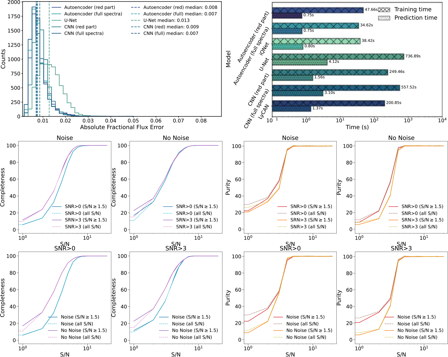
The median AFFE (see Fig. 1) for all models ranges between
 $0.007$
and
 $0.013$
. The autoencoders show the best compromise between performance and computational time, with a training time 30 times and prediction time 2 times lower than more complex architectures (see Fig. 1).
Performances of the models. Top row: histograms of the AFFE (left) and computational times (right) of the models used for the continuum fitting. Bottom row: completeness (left) and purity (right) curves for the models used for the line detection. Here, S/N refers to the lines and SNR to the median value over the whole wavelength range.

Figure 1 Long description
Panel A: A histogram displays the absolute fractional flux error (AFFE) for different models, including Autoencoder, U-Net, and CNN, with both red part and full spectra variations. The x-axis represents the AFFE, and the y-axis represents the counts. Panel B: A bar chart shows the computational times for training and prediction of the models. The x-axis represents the time in seconds, and the y-axis lists the models. Panel C: Line graphs illustrate the completeness of line detection for different signal-to-noise ratios (S/N) and signal-to-noise ratios over the whole wavelength range (SNR), with and without noise. The x-axis represents the S/N, and the y-axis represents completeness in percent. Panel D: Line graphs show the purity of line detection under similar conditions as Panel C. The x-axis represents the S/N, and the y-axis represents purity in percent.
3.2. Line detection
For the line detection (Mangola et al. Reference Mangola, Pistis, Fumagalli and Fossati2025, in prep.), we trained two models based on the U-Net architecture. A model was trained seeing only the (continuum-)normalized flux, while the second was trained seeing also the noise as a secondary channel. We also tested the effects on the performances if the models are trained on spectra with a median signal-to-noise ratio of the spectrum (hereafter SNR) above 3 or the full sample. Figure 1 shows the completeness and purity curves for the line detections as a function of the signal-to-noise ratio of the lines (hereafter S/N) for different models. Letting the model seeing the noise improves the purity for lines with S/N lower than 3, reducing at the same time the completeness in the same range. Training the models on the whole SNR range improves both completeness and purity.
4. Conclusions
All models trained for the continuum fitting can reproduce the true underlying continuum within 1% error. The best compromise between performance (low error) and computational time is given by the autoencoder.
The U-Net used to detect absorption features in the spectra are able to reach 90% on both completeness and purity for lines with
 $\mathrm{S/N} \approx 3$
. Moreover, training on the full sample without a selection on the SNR of the spectra improves both completeness and purity.
This research has been supported by the European Union – Next Generation EU, Mission 4, Component 1 CUP H53D23011030001.



 Open access

