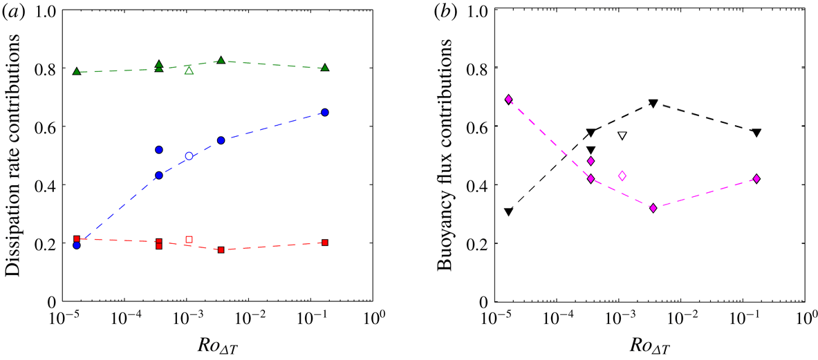
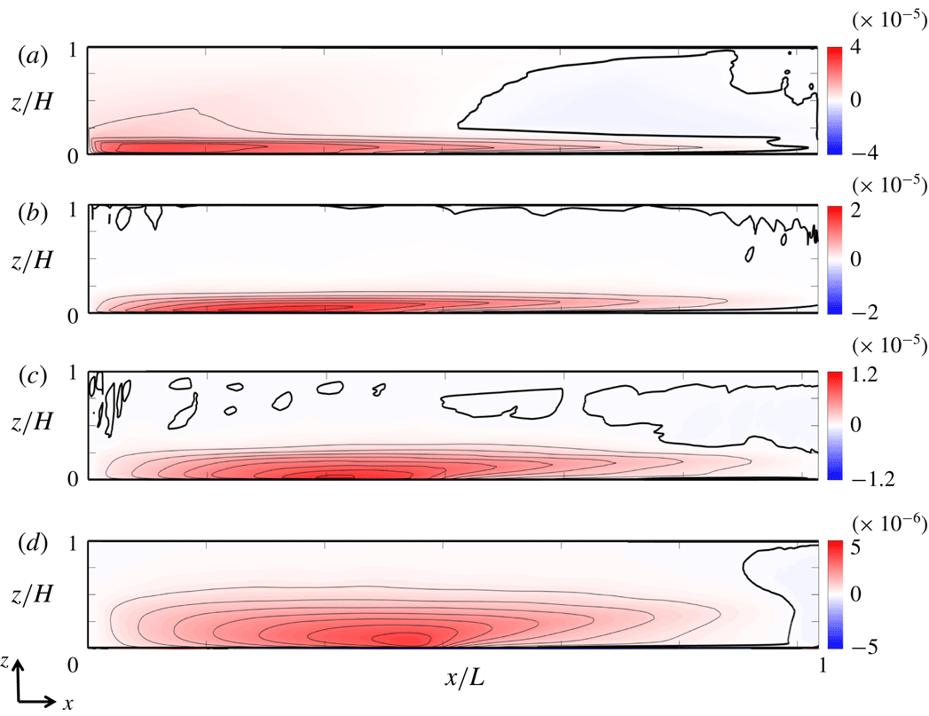
1 Introduction
Circulation of the oceans involves an enormous range of length scales, from the microscales of turbulent dissipation and mixing through submesoscale structures such as fronts and high-latitude deep convection, to quasi-geostrophic Rossby waves, baroclinic eddies, boundary currents and basin-scale gyre recirculation. The transport of heat and buoyancy involves a coupling of near-surface, quasi-horizontal recirculation with deep overturning circulation, and with surface buoyancy fluxes. In the North Atlantic, the ocean circulation transports an estimated 0.6 PW of heat poleward through latitude
 $23\,^{\circ }\text{N}$
. In the northern subpolar regions of the Atlantic, heat (and buoyancy) loss at the surface produces cold dense water, leading to deep chimney convection to depths of 1000–2000 m (Killworth Reference Killworth1983; Marshall & Schott Reference Marshall and Schott1999; Pickart, Torres & Clarke Reference Pickart, Torres and Clarke2001; Våge et al.
Reference Våge, Pickart, Thierry, Reverdin and Lee2009), the associated cooling contributing to a downwelling limb of the overturning circulation and the formation of North Atlantic Deep Water (Talley Reference Talley2003). Global ocean models show that 40–60 % of the northward heat transport in the North Atlantic occurs near the surface through the large-scale gyres and associated boundary currents, with the remaining transport occurring through circulation at depth (Boccaletti et al.
Reference Boccaletti, Ferrari, Adcroft, Ferreira and Marshall2005; Ferrari & Ferreira Reference Ferrari and Ferreira2011). Irrespective of the magnitude of the vertical convective heat transport, it is not clear whether deep convection plays a role in governing the basin heat transport or whether it is slave to the large-scale mean circulation, as implied by the early Robinson–Stommel scaling of quasi-geostrophic upper ocean circulation coupled to vertical advection and diffusion in the subtropical thermocline (Robinson & Stommel Reference Robinson and Stommel1959; Robinson Reference Robinson1960; Stommel Reference Stommel1962). The dynamics of the flow with coupled deep vertical convection and horizontal, largely quasi-geostrophic circulation of the North Atlantic can be found in ocean general circulation models. However, these use parametrisations of vertical convection and the coupling has not been examined through simulations with fully resolved convection and turbulence.
Within regions of deep ocean convection, the sinking of small-scale cold plumes of order 1 km across is thought to create mixed patches, referred to as ‘chimneys’, which are observed to be tens to hundreds of kilometres across (Jones & Marshall Reference Jones and Marshall1993; Maxworthy & Narimousa Reference Maxworthy and Narimousa1994; Send & Marshall Reference Send and Marshall1995; Coates & Ivey Reference Coates and Ivey1997; Marshall & Schott Reference Marshall and Schott1999). The horizontal density gradient between the region of deep convective cooling in the mixed patch and the surrounding water leads to a cyclonic geostrophic surface current, baroclinic instability and eddies, which have diameters of order 10 km. The small-scale plumes are predicted to be affected by Coriolis accelerations, with radial convergence near the surface leading to cyclonic relative vorticity and eventual divergence at depth producing anticyclonic motion (Helfrich Reference Helfrich1994; Maxworthy & Narimousa Reference Maxworthy and Narimousa1994; Marshall & Schott Reference Marshall and Schott1999). The downward transport of water in the plumes is thought to be largely balanced by upwelling around the plumes, giving small net vertical mass flux within the chimney. The theoretical modelling for a horizontally homogeneous region of convection predicts that the convection under ocean conditions would be controlled by a local inertia–buoyancy balance rather than a geostrophic balance. However, direct measurements of deep convection are sparse due to the remote and difficult conditions in the subpolar regions.
Downwelling of dense water is also predicted to occur near side boundaries (Marotzke & Scott Reference Marotzke and Scott1999; Pedlosky Reference Pedlosky2003; Spall Reference Spall2003; Cessi & Wolfe Reference Cessi and Wolfe2009; Cenedese Reference Cenedese2012). Marginal sea models indicate that the location of the mean sinking may be determined by a balance between atmospheric cooling and ocean eddy heat flux (Spall Reference Spall2010, Reference Spall2011). Buoyancy forcing is crucial to the sinking, and modelling evidence indicates that it is also essential to the global overturning, with idealised global ocean models suggesting that surface buoyancy forcing is an important input to the Southern Ocean circulation (Morrison, Hogg & Ward Reference Morrison, Hogg and Ward2011; Morrison, Frölicher & Sarmiento Reference Morrison, Frölicher and Sarmiento2015). Observations (Oort, Anderson & Peixoto Reference Oort, Anderson and Peixoto1994), ocean state estimates (Zemskova, White & Scotti Reference Zemskova, White and Scotti2015) and idealised ocean models (Saenz et al. Reference Saenz, Hogg, Hughes and Griffiths2012) show that the generation of available potential energy by surface buoyancy fluxes may provide as much power to the mechanical energy budget of the circulation as does wind stress. Nevertheless, there is significant uncertainty in large-scale ocean model results, as these models do not fully resolve small-scale convection dynamics and generally do not fully resolve either the kinetic or potential energy budgets, instead using mixing rates dependent on a subgrid-scale parametrised diapycnal diffusivity for density and the kinetic energy dissipation dependent on a parametrised viscosity from turbulence closure schemes.
An alternative approach that can assist in the exploration of the flow dynamics and complement ocean models is to use principles of dynamical similarity to scale the planetary mechanisms operating at large length scale (notably Coriolis accelerations and the meridional gradient of surface heating), while fully resolving the small scales of flow, such that all important mechanisms are allowed to operate within a computationally practical range of resolved length scales (Vreugdenhil, Gayen & Griffiths Reference Vreugdenhil, Gayen and Griffiths2016). This approach is similar to that relied upon in many laboratory studies of the dynamics of rotating convection or stratified circulation. In the case of an applied lateral gradient of surface temperature, the basin scale
 $L$
and basin-scale forcing
 $\unicode[STIX]{x0394}T$
are represented by a horizontal Rayleigh number,
 $Ra$
. Strong buoyancy forcing (
 $Ra>10^{11}$
) leads to a thermal boundary layer at the forcing surface that includes a mixed surface layer formed by convective turbulence (Mullarney, Griffiths & Hughes Reference Mullarney, Griffiths and Hughes2004; Gayen et al.
Reference Gayen, Griffiths, Hughes and Saenz2013; Gayen, Griffiths & Hughes Reference Gayen, Griffiths and Hughes2014; Vreugdenhil et al.
Reference Vreugdenhil, Gayen and Griffiths2016). The circulation and heat throughput are governed by Reynolds stress in an inertia–buoyancy balance, but are otherwise like the laminar viscous flow seen at smaller values of the Rayleigh number (Rossby Reference Rossby1965). The circulation can be geostrophic at large scales, including gyres, boundary currents and baroclinic instability (Park & Whitehead Reference Park and Whitehead1999; Vreugdenhil, Griffiths & Gayen Reference Vreugdenhil, Griffiths and Gayen2017).
Direct numerical simulations (DNS) for a similar rectangular basin and an applied horizontal surface temperature difference, at horizontal Rayleigh number
 $Ra\sim 10^{12}$
(Vreugdenhil et al.
Reference Vreugdenhil, Gayen and Griffiths2016), show a transition from a weakly rotating (effectively non-rotating) regime to a ‘strong rotation’ regime. In the latter the strength of the circulation and the total heat throughput are controlled by thermal wind balance of the quasi-horizontal flow coupled to vertical diffusion–advection balance, in the thermal boundary layer. The results were consistent with regimes earlier identified in theoretical analysis of a cylindrical geometry with a radial surface temperature gradient, in which flow regimes were related to the relative thicknesses of the Ekman and thermal boundary layers (Hignett, Ibbetson & Killworth Reference Hignett, Ibbetson and Killworth1981): strong rotation gives a relatively thin Ekman layer, which leaves the thermal boundary layer inviscid and geostrophic. The geostrophic balance inhibits radial circulation and heat transport. A numerical model of convective overturning in a re-entrant zonal channel (for a relatively small value of the Rayleigh number, a laminar boundary layer and parametrised friction) shows that, when baroclinic instability is allowed, eddies tend to dominate the across-channel heat transport (Barkan, Winters & Llewellyn Smith Reference Barkan, Winters and Llewellyn Smith2013). The DNS results for the rectangular basin, in which side boundaries present barriers to east–west (zonal) flow, are consistent with the Hignett et al. (Reference Hignett, Ibbetson and Killworth1981) analysis, despite the occurrence of boundary currents and baroclinic instability. The DNS results are also consistent with the hypothesis of Robinson & Stommel (Reference Robinson and Stommel1959), Robinson (Reference Robinson1960) and Stommel (Reference Stommel1962) (see also Winton Reference Winton1995; Park & Whitehead Reference Park and Whitehead1999), which assumed thermal wind balance of the mean circulation in the North Atlantic coupled to a balance of upwelling and vertical diffusion through the subtropical ocean thermocline. Nevertheless, heat transport through the subpolar gyre may be governed by baroclinic eddy transport and convective sinking, potentially largely at the boundaries (Spall Reference Spall2010, Reference Spall2011). However, in the Robinson–Stommel scaling the diffusive and convective regions must be coupled, and the dynamics in either of these regions could dominate in governing the overall heat transport.
Previous descriptions of rotating convection in terms of the ratio of boundary layer thicknesses (Hignett et al.
Reference Hignett, Ibbetson and Killworth1981; Hussam, Tsai & Sheard Reference Hussam, Tsai and Sheard2014; Vreugdenhil et al.
Reference Vreugdenhil, Gayen and Griffiths2016) become unsuitable at strong rotation, as Ekman friction becomes a minor factor. The thermal boundary layer is overwhelmingly geostrophic and flow is better described by a convective Rossby number for the inertial flow (Vreugdenhil et al.
Reference Vreugdenhil, Griffiths and Gayen2017). For the case of an imposed buoyancy flux, the Rossby number can be defined as
 $Ro=U/fL=B^{1/2}/f^{3/2}L$
, where
 $B$
is the buoyancy flux per unit area,
 $f$
is the Coriolis parameter and
 $U=(B/f)^{1/2}$
is a velocity scale for the thermal wind. The ‘geostrophic regime’ occurs at
 $Ro<10^{-1}$
(while noting that the small-scale vertical convection and boundary layer turbulence remain strongly ageostrophic). Furthermore, experiments with imposed heat flux (Vreugdenhil et al.
Reference Vreugdenhil, Griffiths and Gayen2017) showed evidence of a third dynamical regime at very strong rotation (or weak buoyancy forcing,
 $Ro<10^{-3}$
), where the dynamics of the chimney convection may control the overall temperature difference and magnitude of the mean circulation. Local fluid accelerations and an effectively non-rotating momentum balance may dominate the chimney convection, and this non-rotating balance has been predicted to apply under North Atlantic conditions (Jones & Marshall Reference Jones and Marshall1993; Maxworthy & Narimousa Reference Maxworthy and Narimousa1994). If the chimneys (rather than the geostrophic parts of the flow) were to govern the overall basin heat transport in the ocean, then the non-rotating convection dynamics would be a strong influence on the global scale.
The recent DNS (Vreugdenhil et al.
Reference Vreugdenhil, Gayen and Griffiths2016) showed that it is feasible to model large-scale geostrophic circulation while resolving small-scale convection and turbulence microscales responsible for dissipation and mixing, albeit in a simple idealised geometry. Here we report more extensive insights from the same simulations, along with a solution for a value of the horizontal Rayleigh number an order of magnitude larger (
 $Ra\sim 10^{13}$
). The problem set-up and scaling theory are outlined in § 2, and the DNS model set-up is outlined in § 3. In § 4 we examine the mass transport by convective chimneys, mean overturning circulation and horizontal quasi-geostrophic flow. The heat transport associated with the mean and fluctuating flow is investigated in § 5. In § 6 the spatial distribution of viscous dissipation and mixing of density are reported. Discussion is in § 7 and concluding remarks are given in § 8. In focusing on the structure and role of convection, we continue to use the simplified case of buoyancy-forced flow on an
 $f$
-plane. The effects of surface wind stress, variation of the Coriolis parameter with latitude and Sverdrup flow will all be included in future steps towards understanding the role of turbulence and small-scale convection in ocean dynamics.
2 Model set-up and scaling solutions
The set-up of the problem is the same as that presented in Vreugdenhil et al. (Reference Vreugdenhil, Gayen and Griffiths2016). The domain is a rotating, rectangular basin of length
 $L$
, width
 $W$
and height
 $H$
(figure 1) with base and top boundaries that are planar and horizontal (gravitational acceleration
 $g$
is vertically downwards). All boundaries are impermeable and all but the base are adiabatic. A no-slip condition is imposed on all boundaries for most solutions, excepting one comparator run in which free-slip conditions are imposed at each of the four vertical boundaries. A temperature
 $T_{h}$
is imposed on one half of the length of the base and a lower temperature
 $T_{c}$
is imposed on the other half, thereby applying a horizontal temperature difference
 $\unicode[STIX]{x0394}T=T_{h}-T_{c}$
along the same horizontal surface. The basin rotates in the anticlockwise direction at angular speed
 $\unicode[STIX]{x1D6FA}$
about a vertical axis, giving a uniform Coriolis parameter
 $f=2\unicode[STIX]{x1D6FA}$
. The total volume and horizontal area of the basin are denoted by
 ${\mathcal{V}}$
and
 ${\mathcal{A}}$
.
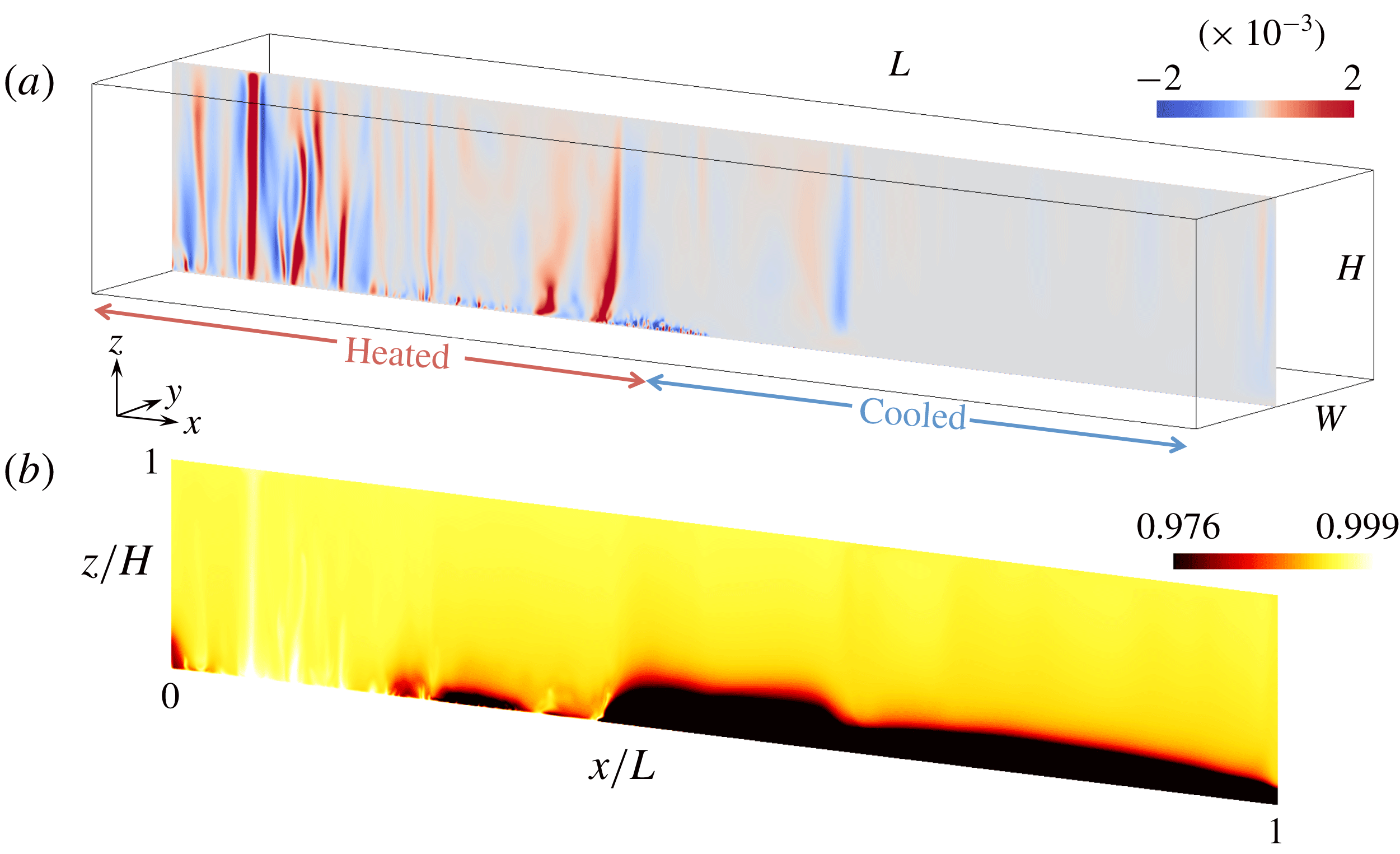
Geometry of the problem and sample solutions from the DNS. The left half of the bottom boundary is warm and the right half is cool. Overlaid in (a) is a snapshot of the solution showing vertical velocity
 $w/\sqrt{g\unicode[STIX]{x1D6FC}\unicode[STIX]{x0394}TL}$
for
 $Ra=7.4\times 10^{12}$
and
 $Ro_{\unicode[STIX]{x0394}T}=1.1\times 10^{-3}$
on the vertical plane
 $y/W=0.45$
. Panel (b) shows the corresponding normalised temperature
 $(T-T_{c})/\unicode[STIX]{x0394}T$
. Colour scales are chosen to highlight the plume convection structures and interior temperatures and therefore do not show the much stronger stratification in the stably stratified parts of the boundary layer (dark region).

The governing equations are assumed to be the incompressible, Boussinesq but non-hydrostatic Navier–Stokes momentum equation in the rotating coordinate frame, along with the continuity equation and conservation of heat:
 $$\begin{eqnarray}\left.\begin{array}{@{}c@{}}\displaystyle Pr^{-1}\left(\frac{\text{D}\hat{\boldsymbol{u}}}{\text{D}\hat{t}}+\unicode[STIX]{x1D735}\hat{p}\right)=Ra\hat{T}\boldsymbol{k}-E^{-1}\boldsymbol{k}\times \hat{\boldsymbol{u}}+\unicode[STIX]{x1D6FB}^{2}\hat{\boldsymbol{u}},\\ \displaystyle \unicode[STIX]{x1D735}\boldsymbol{\cdot }\hat{\boldsymbol{u}}=0,\quad \frac{\text{D}\hat{T}}{\text{D}\hat{t}}=\unicode[STIX]{x1D6FB}^{2}\hat{T},\end{array}\right\}\end{eqnarray}$$
where the bold font indicates vectors and hats denote quantities that have been non-dimensionalised by length
 $L$
, time
 $L^{2}/\unicode[STIX]{x1D705}$
, temperature difference
 $\unicode[STIX]{x0394}T$
or mass
 $\unicode[STIX]{x1D70C}_{r}L^{3}$
. The dimensionless velocity has components
 $\hat{\boldsymbol{u}}=(u,v,w)$
, time is
 $\hat{t}$
, the pressure deviation from the hydrostatic is
 $\hat{p}$
, the temperature is
 $\hat{T}=(T-T_{c})/\unicode[STIX]{x0394}T$
and
 $\boldsymbol{k}$
is a unit upward vector. The governing dimensionless parameters are the Rayleigh, Ekman and Prandtl numbers, along with the vertical and horizontal aspect ratios,
 $$\begin{eqnarray}Ra=\frac{g\unicode[STIX]{x1D6FC}\unicode[STIX]{x0394}TL^{3}}{\unicode[STIX]{x1D708}\unicode[STIX]{x1D705}},\quad E=\frac{\unicode[STIX]{x1D708}}{fL^{2}},\quad Pr=\frac{\unicode[STIX]{x1D708}}{\unicode[STIX]{x1D705}},\quad A_{x}=\frac{H}{L},\quad A_{y}=\frac{W}{L},\end{eqnarray}$$
respectively, where the fluid has kinematic viscosity
 $\unicode[STIX]{x1D708}$
, thermal diffusivity
 $\unicode[STIX]{x1D705}$
, expansion coefficient
 $\unicode[STIX]{x1D6FC}$
and specific heat
 $c_{p}$
, all assumed constant. The density is assumed to be a linear function of temperature.
Further dimensionless parameters of primary physical importance can be constructed from the parameters in (2.2). For small Rayleigh numbers, the (laminar) flow regimes (in a rotating cylinder with radial temperature gradient applied at its base) have been delineated by ranges of the ratio
 $Q\sim (\unicode[STIX]{x1D6FF}_{0}/\unicode[STIX]{x1D6FF}_{E})^{2}$
, defined as the square of the ratio of the thermal boundary layer thickness
 $\unicode[STIX]{x1D6FF}_{0}$
in the non-rotating case (hence the subscript zero) to the Ekman layer thickness
 $\unicode[STIX]{x1D6FF}_{E}$
(Hignett et al.
Reference Hignett, Ibbetson and Killworth1981). As the rotation rate is increased, the flow transitions from the inertial, effectively non-rotating regime (in which the Ekman layer is thicker than the thermal boundary layer) into a regime having the Ekman layer much thinner than the thermal boundary layer, thereby leaving most of the thermal boundary layer dominated by geostrophic thermal wind balance. The inviscid scaling gives
 $\unicode[STIX]{x1D6FF}_{0}\sim L(RaPr)^{-1/5}$
(Hughes et al.
Reference Hughes, Griffiths, Mullarney and Peterson2007; Gayen et al.
Reference Gayen, Griffiths and Hughes2014), the Ekman layer thickness is
 $\unicode[STIX]{x1D6FF}_{E}\sim LE^{1/2}$
and the square of their ratio becomes
 $Q=(RaPr)^{-2/5}E^{-1}$
. Vreugdenhil et al. (Reference Vreugdenhil, Gayen and Griffiths2016) showed that the inviscid parameter
 $QPr$
can be used to delineate regimes for differing rotation rates with a turbulent boundary layer at large Rayleigh numbers.
When
 $QPr=0$
, the flow is in the non-rotating regime, and when
 $QPr\gg 1$
(and
 $\unicode[STIX]{x1D6FF}<H$
), it is in the ‘strong rotation’ regime, which we also refer to as the geostrophic boundary layer regime. However, as the bulk of the thermal boundary layer is inviscid in the rotating flow, it is physically more meaningful to characterise the flow in terms of a Rossby number
 $Ro\sim U/fL$
(where the velocity
 $U$
characterises the thermal boundary layer flow) rather than the thickness of the Ekman layer. This convective Rossby number describes the relative strengths of buoyancy and rotation. For laboratory experiments with imposed heat flux, Vreugdenhil et al. (Reference Vreugdenhil, Griffiths and Gayen2017) show that the scale
 $U=(B/f)^{1/2}$
is a suitable choice (with
 $B$
the imposed buoyancy flux). The Rossby number relates to the previous scaling as
 $Ro=(QPr)^{-3/2}$
. The geostrophic boundary layer regime is then found at
 $Ro\ll 10^{-1}$
, where the induced temperature difference
 $\unicode[STIX]{x0394}T$
, when expressed relative to the temperature difference
 $\unicode[STIX]{x0394}T_{0}$
of the corresponding non-rotating case, varies as
 $\unicode[STIX]{x0394}T/\unicode[STIX]{x0394}T_{0}\sim Ro^{-1/6}$
. At
 $Ro>10^{-1}$
the non-rotating scaling applies.
For the case of an imposed temperature difference, examined here, there are again several velocity scales available to define the Rossby number, including the buoyancy–inertia scale
 $U\sim (g\unicode[STIX]{x1D6FC}\unicode[STIX]{x0394}TL)^{1/2}=(\unicode[STIX]{x1D705}/L)(RaPr)^{1/2}$
, the thermal wind velocity
 $U=g\unicode[STIX]{x1D6FC}\unicode[STIX]{x0394}TH/fL=RaE^{2}Pr^{-1}(H/L)^{-2}$
and the geostrophic boundary layer scaling result
 $U\sim (\unicode[STIX]{x1D705}/L)(RaE)^{2/3}$
. It is not critical which is chosen because we simply wish to rewrite the scaling in terms of a Rossby number: the scaling dependence on rotation or buoyancy forcing remains unchanged by this choice. Here we use the latter, which is the result of coupling thermal wind balance in the thermal boundary layer with a balance of vertical upwelling and diffusion through the boundary layer (Robinson & Stommel Reference Robinson and Stommel1959; Stommel Reference Stommel1962; Vreugdenhil et al.
Reference Vreugdenhil, Gayen and Griffiths2016). The convective Rossby number becomes
 $$\begin{eqnarray}Ro_{\unicode[STIX]{x0394}T}=Ra^{2/3}E^{5/3}/Pr.\end{eqnarray}$$
Hence
 $Ro_{\unicode[STIX]{x0394}T}=(QPr)^{-5/3}$
. Given that scaling analysis and DNS results (Vreugdenhil et al.
Reference Vreugdenhil, Gayen and Griffiths2016) show the geostrophic regime at
 $QPr>O(10)$
, this result can now be restated as a transition in the thermal boundary layer flow at
 $Ro_{\unicode[STIX]{x0394}T}\approx 10^{-1}$
, from Reynolds stress control (non-rotating) to geostrophic control. At small
 $Ro_{\unicode[STIX]{x0394}T}$
the new scaling implies thermal boundary layer thickness
 $\unicode[STIX]{x1D6FF}$
and velocity
 $U$
, and dimensionless heat transport
 $Nu$
,
 $$\begin{eqnarray}\left.\begin{array}{@{}c@{}}\unicode[STIX]{x1D6FF}\sim L(RaPrRo_{\unicode[STIX]{x0394}T})^{-1/5},\\ U\sim (\unicode[STIX]{x1D705}/L)(RaPrRo_{\unicode[STIX]{x0394}T})^{2/5},\\ Nu\sim (RaPrRo_{\unicode[STIX]{x0394}T})^{1/5},\end{array}\right\}\end{eqnarray}$$
where
 $Nu=FL/\unicode[STIX]{x1D70C}_{r}c_{p}\unicode[STIX]{x1D705}\unicode[STIX]{x0394}T$
is the Nusselt number (Rossby Reference Rossby1965; Gayen et al.
Reference Gayen, Griffiths and Hughes2014),
 $\unicode[STIX]{x1D70C}_{r}$
is a reference density,
 $c_{p}$
is the specific heat and
 $F$
is the resulting heat flux per unit area averaged over the heated half of the base. Thus the effect of rotation is to reduce the heat transport according to
 $Nu/Nu_{0}\sim Ro_{\unicode[STIX]{x0394}T}^{1/5}$
, where
 $Nu_{0}$
is the Nusselt number of the non-rotating case. In terms of the raw variables, the scaling gives
 $Ro_{\unicode[STIX]{x0394}T}=[g\unicode[STIX]{x1D6FC}\unicode[STIX]{x0394}T\unicode[STIX]{x1D705}^{1/2}/(f^{5/2}L^{2})]^{2/3}$
and
 $U\approx (\unicode[STIX]{x1D705}/L)[g\unicode[STIX]{x1D6FC}\unicode[STIX]{x0394}TL/\unicode[STIX]{x1D705}f]^{2/3}$
.
The three-dimensional mean circulation is assumed to be adequately represented by two-dimensional streamfunctions in horizontal
 $\unicode[STIX]{x1D713}_{H}$
and vertical
 $\unicode[STIX]{x1D713}_{vert}$
planes. The corresponding volume transport is given by appropriate integrations of the streamfunctions over the basin depth (for horizontal streamfunction) or width (for vertical streamfunction). The zonally integrated overturning transport is then
 $$\begin{eqnarray}\unicode[STIX]{x1D709}_{vert}=\int _{0}^{W}\unicode[STIX]{x1D713}_{vert}\,\text{d}y,\end{eqnarray}$$
where
 $\unicode[STIX]{x1D713}_{vert}$
is defined by
 $(u,w)=(\unicode[STIX]{x2202}\unicode[STIX]{x1D713}_{vert}/\unicode[STIX]{x2202}z,-\unicode[STIX]{x2202}\unicode[STIX]{x1D713}_{vert}/\unicode[STIX]{x2202}x)$
. The horizontal depth-integrated transport within the thermal boundary layer is
 $$\begin{eqnarray}\unicode[STIX]{x1D709}_{H}=\int _{0}^{\unicode[STIX]{x1D6FF}}\unicode[STIX]{x1D713}_{H}\,\text{d}z,\end{eqnarray}$$
where
 $\unicode[STIX]{x1D713}_{H}$
is defined by
 $(u,v)=(\unicode[STIX]{x2202}\unicode[STIX]{x1D713}_{H}/\unicode[STIX]{x2202}y,-\unicode[STIX]{x2202}\unicode[STIX]{x1D713}_{H}/\unicode[STIX]{x2202}x)$
at each level. The maximum value of the baroclinic component of the horizontal transport in the boundary layer is defined as
 $$\begin{eqnarray}\unicode[STIX]{x1D709}_{B}=\int _{0}^{\unicode[STIX]{x1D6FF}}\unicode[STIX]{x1D713}_{H}\,\text{d}z-(\unicode[STIX]{x1D6FF}/H)\int _{0}^{H}\unicode[STIX]{x1D713}_{H}\,\text{d}z,\end{eqnarray}$$
where the second term on the right-hand side is the contribution of the barotropic flow.
Established scaling for the non-rotating case gives the overturning transport, in the inertial boundary layer regime at large Rayleigh number, as
 $$\begin{eqnarray}\unicode[STIX]{x1D709}_{0}=c_{0}\unicode[STIX]{x1D705}W(RaPr)^{1/5},\end{eqnarray}$$
with
 $c_{0}$
a prefactor of
 $O(1)$
(Hughes et al.
Reference Hughes, Griffiths, Mullarney and Peterson2007; Gayen et al.
Reference Gayen, Griffiths and Hughes2014). When rotation is strong relative to buoyancy forcing, the diffusive–thermal wind thermocline scaling gives
 $U\sim (\unicode[STIX]{x1D705}/L)(RaE)^{2/3}$
and the Rossby number relations (2.4). These imply an overturning streamfunction due to the boundary layer flow (excluding additional mean overturning in the interior associated with turbulent entrainment into plume convection (Hughes et al.
Reference Hughes, Griffiths, Mullarney and Peterson2007))
 $\unicode[STIX]{x1D713}_{vert}\sim U\unicode[STIX]{x1D6FF}\sim \unicode[STIX]{x1D705}(RaE)^{1/3}$
and a baroclinic contribution to the horizontal streamfunction in the boundary layer
 $$\begin{eqnarray}\unicode[STIX]{x1D713}_{vert}\sim \unicode[STIX]{x1D705}(RaPrRo_{\unicode[STIX]{x0394}T})^{1/5},\quad \unicode[STIX]{x1D713}_{B}\sim \unicode[STIX]{x1D705}(W/L)(RaPrRo_{\unicode[STIX]{x0394}T})^{2/5}.\end{eqnarray}$$
The associated integrated transports are
 $\unicode[STIX]{x1D709}_{vert}\sim \unicode[STIX]{x1D713}_{vert}W$
and
 $\unicode[STIX]{x1D709}_{H}\sim \unicode[STIX]{x1D713}_{H}\unicode[STIX]{x1D6FF}$
, both of which become
 $$\begin{eqnarray}\unicode[STIX]{x1D709}_{vert}\sim \unicode[STIX]{x1D709}_{B}\sim \unicode[STIX]{x1D705}W(RaPrRo_{\unicode[STIX]{x0394}T})^{1/5},\end{eqnarray}$$
where we recall that the corresponding result (2.8) for the non-rotating case has
 $\unicode[STIX]{x1D709}_{vert,0}=\unicode[STIX]{x1D709}_{H,0}\sim \unicode[STIX]{x1D705}W(RaPr)^{1/5}$
.
Finally, the ratio of the buoyancy time scale
 $\unicode[STIX]{x1D70F}_{b}=(L/g\unicode[STIX]{x1D6FC}\unicode[STIX]{x0394}T)^{1/2}$
to the inertial period
 $f^{-1}$
can be expressed in terms of the Rossby number (2.3),
 $f\unicode[STIX]{x1D70F}_{b}=Ro_{\unicode[STIX]{x0394}T}^{-3/4}(E/Pr)^{1/4}$
, from which it can be seen that for
 $E\ll 1$
and
 $Ro_{\unicode[STIX]{x0394}T}<O(1)$
the buoyancy period (on which time averaging is based) is very much longer than the inertial period.
3 Direct numerical simulation methodology
Flow solutions to (2.1) are found for the rotating, rectangular basin (figure 1) with aspect ratios
 $A_{x}=H/L=0.16$
and
 $A_{y}=W/L=0.24$
. These are chosen to match past non-rotating laboratory experiments (Mullarney et al.
Reference Mullarney, Griffiths and Hughes2004; Stewart, Hughes & Griffiths Reference Stewart, Hughes and Griffiths2011; Griffiths, Hughes & Gayen Reference Griffiths, Hughes and Gayen2013), previous DNS studies of non-rotating convection (Griffiths et al.
Reference Griffiths, Hughes and Gayen2013; Gayen et al.
Reference Gayen, Griffiths, Hughes and Saenz2013, Reference Gayen, Griffiths and Hughes2014), and rotating laboratory experiments (Vreugdenhil et al.
Reference Vreugdenhil, Griffiths and Gayen2017). In order to avoid a discontinuity in temperature halfway along the length, the temperature profile on the base is a hyperbolic tangent function in the long (
 $x$
) direction, the gradient being confined to a length scale
 $0.06L$
about the centre
 $x=L/2$
. Thus the system differs from the previous rotating laboratory experiments (which used an imposed input heat flux over one half of the base (Vreugdenhil et al.
Reference Vreugdenhil, Griffiths and Gayen2017)) only in the thermal boundary condition imposed on the heating half of the base. A no-slip condition is imposed on all boundaries for most solutions, excepting one additional run with free-slip conditions imposed at each of the four vertical boundaries.
In all runs presented here, the Prandtl number
 $Pr=5$
, a value that is approximately representative of the average value for water in previous relevant laboratory experiments. A slightly larger (molecular) value would be appropriate for the lower average temperatures of ocean water. A range of Ekman numbers (table 1) were examined for the Rayleigh number value
 $Ra=7.4\times 10^{11}$
and a single, very computationally expensive run was possible for
 $Ra=7.4\times 10^{12}$
. These Rayleigh number values are greater than those required for the equivalent non-rotating case to be in a turbulent, inertial regime (
 $Ra>10^{11}$
). Small-scale turbulent convection creates a mixed layer adjacent to the heated, destabilised region of the base and beneath a remnant stratified part of the thermal boundary layer (Mullarney et al.
Reference Mullarney, Griffiths and Hughes2004; Gayen et al.
Reference Gayen, Griffiths and Hughes2014).
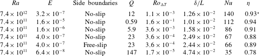
Conditions and key summary results for the simulations. The Rayleigh number
 $Ra$
is varied by changing the buoyancy
 $g\unicode[STIX]{x1D6FC}\unicode[STIX]{x0394}T$
, and the Ekman number
 $E$
is varied by changing the Coriolis parameter
 $f$
. As defined in the text,
 $Q$
is the squared ratio of thermal to Ekman boundary layer thicknesses,
 $Ro_{\unicode[STIX]{x0394}T}$
is the ratio of buoyancy to Coriolis forces (the convective Rossby number),
 $\unicode[STIX]{x1D6FF}/L$
is the measured thermal boundary layer thickness (see § 4.1),
 $Nu$
is dimensionless heat throughput, and
 $\unicode[STIX]{x1D702}$
is mixing efficiency (the starred value of
 $\unicode[STIX]{x1D702}$
is based on viscous dissipation that is not quite in thermal equilibrium,
 $\unicode[STIX]{x1D702}$
still increasing very slowly when the run had to be terminated).

The solution grid had
 $768\times 256\times 256$
cells (for
 $Ra=7.4\times 10^{11}$
) and
 $1536\times 512\times 512$
cells (for
 $Ra=7.4\times 10^{12}$
), clustered near the boundaries in order to resolve the top and bottom Ekman layers of thickness
 $\unicode[STIX]{x1D6FF}_{E}=(2\unicode[STIX]{x1D708}/f)^{1/2}=L(2E)^{1/2}$
and the sidewall Stewartson boundary layers of thickness
 $\unicode[STIX]{x1D6FF}_{S}=(2\unicode[STIX]{x1D708}L^{2}/f)^{1/4}=L(2E)^{1/4}$
. The viscous Stewartson layers on the vertical boundaries bring the boundary velocity to zero, satisfying the no-slip boundary condition (Stewartson Reference Stewartson1957, Reference Stewartson1966; Van Heijst Reference Van Heijst1983; Kunnen et al.
Reference Kunnen, Stevens, Overkamp, Sun, Van Heijst and Clercx2011). Across the basin width, the stretching is small and of the form
 $y(j)=(W/2)(1+\tanh (S_{y}(j-1/N-1/2))/\tanh (S_{y}/2))$
, where
 $j=[1,N]$
,
 $N$
is the total number of grid points,
 $W$
is the basin width and
 $S_{y}=1$
is the stretching factor. The same stretching function is used in the
 $x$
and
 $z$
directions, but the stretching is greater (
 $S_{x}=1.2$
,
 $S_{z}=1.3$
) and shifted so as to be symmetric around the endwall (at the cooled end) and upper boundary. This serves to place more cells in the endwall plume (for the non-rotating case) and in the bottom thermal boundary layer. There is additional clustering in the upper 30 grid points in order to resolve the upper Ekman layer. For the
 $Ra=7.4\times 10^{11}$
cases, there are at least 35 grid points in the thermal boundary layer and at least four grid points in each of the top and bottom Ekman layers, excepting the extremely strong rotation case at
 $E=6.4\times 10^{-8}$
, which only has two grid points in the Ekman layers. For
 $Ra=7.4\times 10^{12}$
there are at least 83 grid points in the thermal boundary layer and seven grid points in each of the top and bottom Ekman layers. Adequate resolution was confirmed by comparison of the local grid spacing
 $\unicode[STIX]{x1D6E5}_{x,y,z}$
to the Batchelor microscale
 $\unicode[STIX]{x1D702}_{b}=(\unicode[STIX]{x1D708}^{3}/\unicode[STIX]{x1D716}^{\ast })^{1/4}Pr^{-1/2}$
(where
 $\unicode[STIX]{x1D716}^{\ast }$
is the local dissipation rate), which always satisfied the criterion
 $[\unicode[STIX]{x1D6E5}_{x},\unicode[STIX]{x1D6E5}_{y},\unicode[STIX]{x1D6E5}_{z}]_{max}\leqslant \unicode[STIX]{x03C0}\unicode[STIX]{x1D702}_{b}$
(Stevens, Verzicco & Lohse Reference Stevens, Verzicco and Lohse2010; Gayen et al.
Reference Gayen, Griffiths and Hughes2014). Finally the most stringent test of adequate resolution is that the overall mechanical energy budget was accurately balanced to within
 $10^{-3}$
of the total volume-integrated dissipation (Gayen et al.
Reference Gayen, Griffiths and Hughes2014), which indicates that the sum of grid cell imbalances is extremely small.
A third-order Runge–Kutta–Wray method was used for time stepping, excepting the viscous terms, for which an alternating direction implicit method was used. The spatial terms were calculated using a second-order finite difference method and a multi-grid pressure solver was used to remove divergence. Variable time steps were employed using a Courant–Friedrichs–Lewy number of unity. The time steps at the larger
 $Ra$
are
 $O(10^{-9})L^{2}/\unicode[STIX]{x1D705}$
.
Solutions were initialised with a uniform water temperature of
 $\hat{T}=0.66$
and allowed to evolve until they reached a (warmer) thermally equilibrated state. Equilibrium was reached on the e-folding time scale
 $\unicode[STIX]{x1D70F}_{e}\approx \unicode[STIX]{x1D6FD}\unicode[STIX]{x1D6FF}H/\unicode[STIX]{x1D705}$
, where
 $\unicode[STIX]{x1D6FF}$
is the thickness of the thermal boundary layer and the prefactor
 $\unicode[STIX]{x1D6FD}=1.4$
is the same as the value previously found in the non-rotating case (Griffiths et al.
Reference Griffiths, Hughes and Gayen2013). The initial temperature was chosen to be colder than the final temperature in order to minimise the time taken to reach equilibrium. Each simulation was thereafter continued for 600 (for
 $Ra=7.4\times 10^{11}$
) or 65 (for
 $Ra=7.4\times 10^{12}$
) buoyancy time scales
 $\unicode[STIX]{x1D70F}_{b}=(L/g\unicode[STIX]{x1D6FC}\unicode[STIX]{x0394}T)^{1/2}$
in order to allow evaluation of mean and fluctuation quantities. Nevertheless, the adjustment accounts for most of the time required. The thermally equilibrated solution for
 $Ra=7.4\times 10^{11}$
and
 $E=4.0\times 10^{-7}$
was further used to initialise the additional run with free-slip vertical boundaries (with all other imposed parameters unchanged). The larger
 $Ra$
was very computationally expensive and hence only one rotation rate could be examined for this Rayleigh number. Thus the results for
 $Ra=7.4\times 10^{11}$
are used to define trends with varying rotation rate and Rossby number, whereas the solution for the higher Rayleigh number is used to examine the effects of an increased range of length scales.
4 Mass transport
4.1 Flow structure and small-scale convection
All of the solutions are highly unsteady. We therefore begin by describing the solutions in terms of instantaneous snapshots of the flow structure, followed by an examination of the time-averaged flow. Emphasis is given to the location of vertical convective transport.
Snapshots of vertical velocity and temperature on a vertical plane are shown for strong rotation (
 $Ra=7.4\times 10^{12}$
,
 $Ro_{\unicode[STIX]{x0394}T}=1.1\times 10^{-3}$
) in figure 1, where velocity is normalised by the simplest scale (
 $\sqrt{g\unicode[STIX]{x1D6FC}\unicode[STIX]{x0394}TL}$
) for buoyancy-driven inertial flow and the temperature difference from the cold boundary is normalised by the imposed
 $\unicode[STIX]{x0394}T$
. The snapshots illustrate the shallow, very small-scale convection within the thermal boundary layer close to
 $\hat{x}\approx 0.5$
, where the boundary layer flow first encounters a destabilising boundary buoyancy flux. These snapshots also show deep, vertically coherent warm plumes in the interior at
 $\hat{x}<0.3$
(figure 1
b), having horizontal scale much larger than the boundary layer convection and strong upward velocities throughout the depth of the box (figure 1
a). In contrast, where the boundary buoyancy flux is stabilising at
 $\hat{x}>0.5$
, there is weak downwelling into the thermal boundary layer and the flow is laminar.
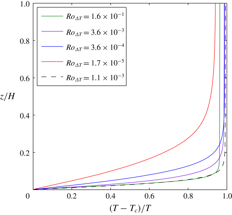
The thermal boundary layer is clearly shown by vertical profiles of temperature above the cooling region of the base (figure 2). Temperature profiles at other locations are similar, and like those in the non-rotating case (Gayen et al.
Reference Gayen, Griffiths and Hughes2014), apart from the presence of a mixed layer in the lower portion of the thermal boundary layer over the heated region of the base. The temperature gradient is stable everywhere outside the mixed layer and the very thin sublayer on the heated region of the base. The thermal boundary layer thickness, defined here as the height encompassing 90 % of the top-to-bottom temperature difference (zonally and time-averaged at
 $\hat{x}=0.75$
), is listed in table 1 and was previously shown to be consistent with the geostrophic scaling (2.4) (Vreugdenhil et al.
Reference Vreugdenhil, Gayen and Griffiths2016). The boundary layer is thinner for smaller Rossby numbers. Outside the boundary layer, the stratification is larger for smaller Rossby numbers.
Vertical profiles of temperature in the cooled half at
 $\hat{x}=0.92$
averaged in the ‘zonal’ direction for
 $Ra=7.4\times 10^{11}$
(no-slip sidewalls, solid curves) and
 $Ra=7.4\times 10^{12}$
(broken curve). Line colour indicates
 $Ro_{\unicode[STIX]{x0394}T}$
.

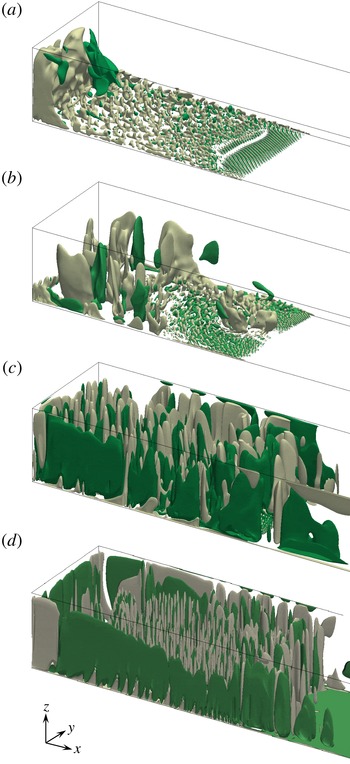
Snapshots of flow structure represented by the shape of two surfaces having fixed vertical velocity for
 $Ra=7.4\times 10^{11}$
and three values of the Rossby number: (a)
 $Ro_{\unicode[STIX]{x0394}T}=1.6\times 10^{-1}$
, (b)
 $Ro_{\unicode[STIX]{x0394}T}=3.6\times 10^{-3}$
, (c)
 $Ro_{\unicode[STIX]{x0394}T}=3.6\times 10^{-4}$
and (d)
 $Ro_{\unicode[STIX]{x0394}T}=1.7\times 10^{-5}$
(all with no-slip sidewalls). Isosurfaces show upward (grey) and downward (green) normalised velocities
 $w/\sqrt{g\unicode[STIX]{x1D6FC}\unicode[STIX]{x0394}TL}$
at values chosen to most effectively illustrate the flow: (a)
 $\pm 3.2\times 10^{-3}$
, (b)
 $\pm 1.6\times 10^{-3}$
, (c)
 $\pm 3.2\times 10^{-4}$
and (d)
 $\pm 3.2\times 10^{-4}$
. Only the region above the heated half of the base is shown; the cooled half extends to the right.

The dependence of flow structure on rotation rate is further illustrated in figure 3, where vertical velocity isosurfaces are shown for several values of the ratio
 $Ro_{\unicode[STIX]{x0394}T}$
of buoyancy forcing to rotation rate. Velocities are again normalised by the buoyancy–inertia scale involving the least assumptions and independent of rotation rate. At
 $Ro_{\unicode[STIX]{x0394}T}>10^{-1}$
(weak rotation, figure 3
a) the flow shows coherent two-dimensional convection rolls aligned with the local flow direction near the leading edge of the heated region. The depth of the boundary layer convection increases with distance downstream and the rolls transition after a short distance to three-dimensional turbulence. The turbulence remains capped by boundary layer stratification except at the end of the basin, where it is carried into a large, full-depth endwall plume. All of these features are similar to those previously reported for the non-rotating case (Mullarney et al.
Reference Mullarney, Griffiths and Hughes2004; Gayen et al.
Reference Gayen, Griffiths and Hughes2014). For strong rotation (shown for
 $Ro_{\unicode[STIX]{x0394}T}=3.6\times 10^{-3}$
in figure 3
b), the onset of boundary layer instability can be seen closer to the leading edge of the heated region of the base, and streamwise rolls are again parallel to the (now deflected and slower) mean flow of the boundary layer and become turbulent within a shorter distance. Full-depth convection, which remains essential in order to maintain the temperature near the top boundary, now involves many vortical plumes, which are broadly distributed over an area at
 $\hat{x}<0.3$
. Thus there is no longer a single endwall plume, although weak upwelling at the endwall persists. With still stronger rotation (
 $Ro_{\unicode[STIX]{x0394}T}=3.6\times 10^{-4}$
and
 $Ro_{\unicode[STIX]{x0394}T}=1.7\times 10^{-5}$
; figure 3
c,d), the vertical convection is confined to the boundary layer in only a very small region and the vortical plumes become more numerous, more widespread and also more coherent between the interior and boundary layer. Under these conditions, there is no longer a scale separation between the small-scale convection in the boundary layer and the vortical coherent plumes. There is broader, slower and less organised downwelling around the upward vortical plumes.
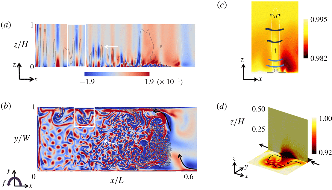
Snapshots of the vertical component of relative vorticity, shown for strong rotation in figure 4, again reveal the small-scale boundary layer convection, its deepening as it is carried along (and across) the basin by the mean flow between
 $\hat{x}\approx 0.5$
and
 $\hat{x}\approx 0.3$
(figure 4
a), and its evolution further ‘downstream’ into deep vortical plumes. The base of each plume is hot compared to the surroundings (figure 1
b and schematic in figure 4
c) due to convergence of warm water (in the heated sublayer below the bulk of the cold, dense boundary layer) into the base of the plume. Vortex stretching in the plumes leads to cyclonic relative vorticity (figure 4
a–c). Higher in the water column, beyond the thermal boundary layer, there is radial divergence in each plume, vortex compression and anticyclonic relative vorticity (Helfrich Reference Helfrich1994; Maxworthy & Narimousa Reference Maxworthy and Narimousa1994; Marshall & Schott Reference Marshall and Schott1999). The horizontal scale of the plumes decreases with increasing rotation rate or decreasing Rossby number.
Vertical component of relative vorticity, normalised by
 $f$
,
 $\unicode[STIX]{x1D714}/f=f^{-1}\unicode[STIX]{x1D735}\times (u,v)$
, for
 $Ra=7.4\times 10^{11}$
and
 $Ro_{\unicode[STIX]{x0394}T}=3.6\times 10^{-4}$
(no-slip) on (a) a vertical plane
 ${\hat{y}}=0.2$
and (b) a horizontal plane
 $\hat{z}=0.01$
(within the thermal boundary layer, outside the Ekman layer). Contour lines in (a) show isosurfaces of upward velocity
 $w/\sqrt{g\unicode[STIX]{x1D6FC}\unicode[STIX]{x0394}TL}=3.2\times 10^{-4}$
(white) and downward velocity
 $w/\sqrt{g\unicode[STIX]{x1D6FC}\unicode[STIX]{x0394}TL}=-3.2\times 10^{-4}$
(black). Black arrows in (b) show the direction of the strongest mean current from the cooled to the heated region. White arrows in (a,b) show the general direction of migration of deep plumes (the area
 $\hat{z}<0.6$
is shown). (c) Zoom showing the plume in the white rectangle in (a), with colours showing temperature
 $\hat{T}$
, white contour showing isosurface of upward velocity
 $w/\sqrt{g\unicode[STIX]{x1D6FC}\unicode[STIX]{x0394}TL}=3.2\times 10^{-4}$
and blue arrows indicating direction of local circulation. (d) Zoom on the sidewall boundary current in the white rectangle in (b) and a vertical plane
 ${\hat{y}}=0.96$
, with colour showing temperature
 $\hat{T}$
. Large black arrows show the direction of the boundary current near the base, and thin arrows show the current in the eddy.

The columnar vortices at rapid rotation shown by the vertical velocity isosurfaces in figure 3 may bear some resemblance to the structures of strongly rotating Rayleigh–Bénard convection (King, Stellmach & Aurnou Reference King, Stellmach and Aurnou2012; Julien et al. Reference Julien, Rubio, Grooms and Knobloch2012, Reference Julien, Aurnou, Calkins, Knobloch, Marti, Stellmach and Vasil2016; Plumley et al. Reference Plumley, Julien, Marti and Stellmach2016). However, it is clear from figure 4 that the columnar vortices are not the same, even locally, because the columns penetrate through or break down a stably stratified boundary layer and a weakly stable stratification in the interior. In addition, the cooling is supplied to the convecting region by horizontal flow (from the cold base) in the boundary layer, setting the present case apart from rotating Rayleigh–Bénard convection.
Relative vorticity (in figure 4
a,b) also highlights a highly unsteady, cold current along the boundary
 ${\hat{y}}=1$
(which we refer to as the ‘eastern’ boundary despite the uniform Coriolis parameter) over the heated region and continuing towards the ‘northern’ endwall (
 $\hat{x}=0$
). This current is in the thermal boundary layer against the base and links to a flow along the opposite sidewall
 ${\hat{y}}=0$
in the cooled region, which crosses the basin near the mid-section (
 $\hat{x}\approx 0.6$
). The mean velocity component
 $v$
in the current across the basin is in thermal wind balance with the temperature gradient in the
 $x$
direction. For free-slip sidewalls the boundary current is narrower and faster, but otherwise there is little difference between the solutions with free- or no-slip conditions. The dense current along the ‘eastern’ boundary undergoes wave and eddy instability that has horizontal scales comparable to the boundary layer Rossby deformation radius and which appear to be a result of baroclinic instability of a local gravitationally stable density gradient (rather than of convection driven by a density inversion). This instability produces cold, anticyclonic eddies surrounded by filaments of cyclonic relative vorticity (figure 4
d). The baroclinic eddies propagate slowly towards the mid-section
 $\hat{x}=0.5$
(in the opposite direction to the mean current), where they disappear in the co-flowing mean motion of a large anticyclonic gyre. The enhanced heat input from the base to the cold eddies enhances small-scale convection in the most weakly stratified, anticyclonic regions of the baroclinic waves. The size of the eddies decreases with increasing rotation rate, approximately proportional to the Rossby radius. Moving from
 $Ro_{\unicode[STIX]{x0394}T}=3.6\times 10^{-4}$
to
 $Ro_{\unicode[STIX]{x0394}T}=1.7\times 10^{-5}$
at fixed Rayleigh number sees a 20-fold decrease in the inertial radius
 $U/f$
(
 ${\sim}Ro_{\unicode[STIX]{x0394}T}$
), a 6.3-fold decrease in the deformation radius
 $\unicode[STIX]{x1D706}\sim \sqrt{g\unicode[STIX]{x1D6FC}\unicode[STIX]{x0394}TL}/f$
(
 ${\sim}(RaPr)^{1/10}Ro^{3/5}$
) and a 4.6-fold decrease in an alternative deformation radius based on the boundary layer depth (
 $\unicode[STIX]{x1D706}_{bl}\sim \sqrt{g\unicode[STIX]{x1D6FC}\unicode[STIX]{x0394}T\unicode[STIX]{x1D6FF}}/f\sim Ro_{\unicode[STIX]{x0394}T}^{1/2}$
). An approximate four-fold decrease in wavelength is observed. Baroclinic eddies are also generated from the current crossing the basin near the mid-section, contributing to lateral transport of water and heat through this section and a mix of geostrophic turbulence and vertical convection in this energetic site.
4.2 Mean circulation
The mean flow is estimated by averaging the velocities over a period of 600 (for
 $Ra=7.4\times 10^{11}$
) or 65 (for
 $Ra=7.4\times 10^{12}$
) buoyancy time scales
 $\unicode[STIX]{x1D70F}_{b}$
, a period that is as long as the solutions could practically be run after reaching the thermally equilibrated state. However, it is long enough to average over all but very low-frequency fluctuations.
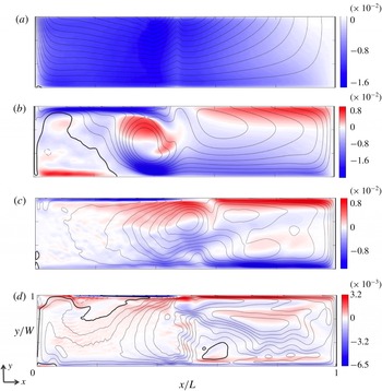
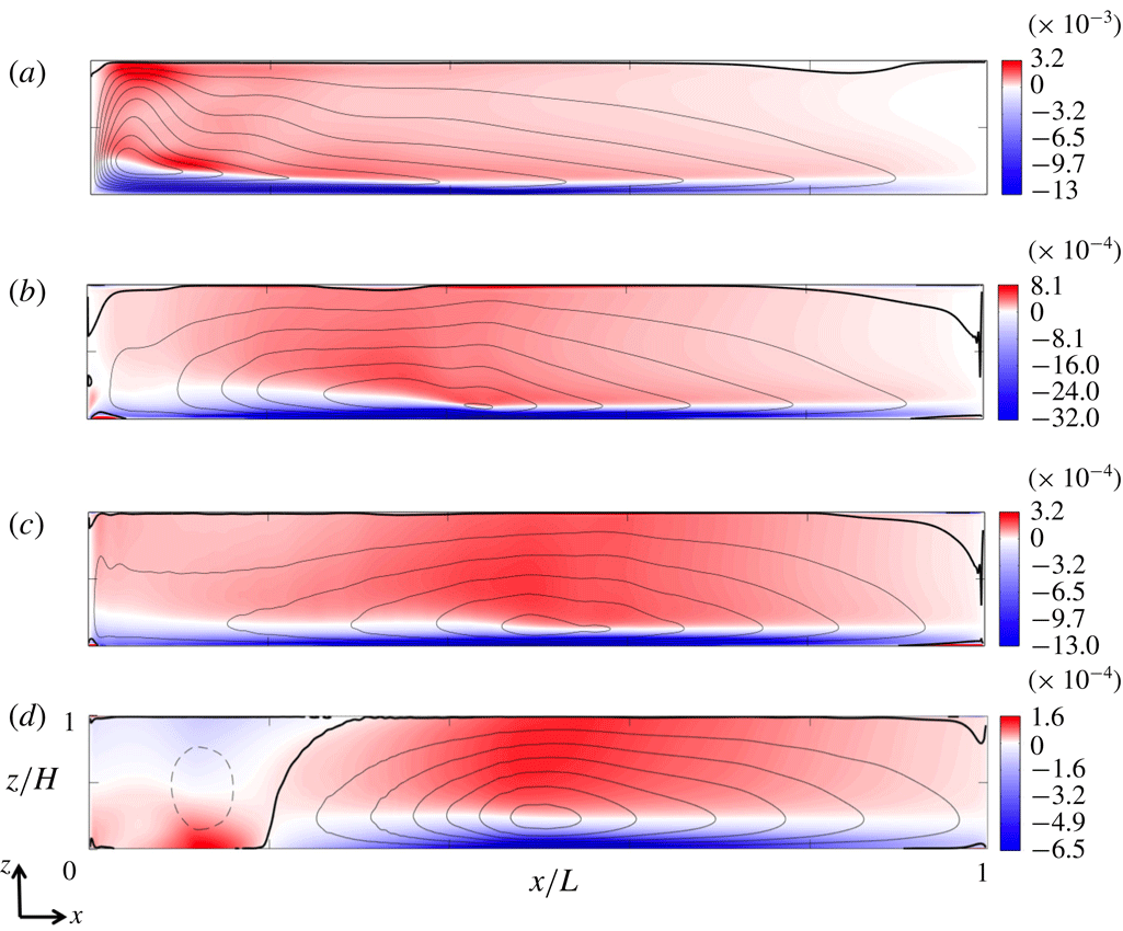
The variation with rotation rate (at a fixed Rayleigh number) of the horizontal mean circulation within the thermal boundary layer is represented in figure 5 by the
 $x$
component of the mean velocity on the plane
 $z=\unicode[STIX]{x1D6FF}/2$
(which is outside the Ekman layer in all cases) and the horizontal streamfunction
 $\unicode[STIX]{x1D713}_{H}$
, defined by
 $(u,v)=(\unicode[STIX]{x2202}\unicode[STIX]{x1D713}_{H}/\unicode[STIX]{x2202}y,-\unicode[STIX]{x2202}\unicode[STIX]{x1D713}_{H}/\unicode[STIX]{x2202}x)$
, calculated on the same plane. The solutions show a mostly uniform flow from the cooled to the heated region at weak rotation and two or three quasi-steady gyres at strong rotation. In particular, for
 $10^{-2}>Ro_{\unicode[STIX]{x0394}T}>10^{-4}$
, an anticyclonic gyre dominates the region of stabilising boundary buoyancy flux. There is a smaller but stronger anticyclonic gyre in the middle region above the destabilising boundary flux, and a strong current across the width of the basin (in the
 $y$
direction) at
 $0.3<\hat{x}<0.4$
. There is weak cyclonic circulation near the endwall of the heated region. At the strongest rotation rate (
 $Ro_{\unicode[STIX]{x0394}T}=1.7\times 10^{-5}$
), there is a general anticyclonic (clockwise) circulation but with a more complicated current near the middle of the basin. Comparison of the solutions at the two Rayleigh numbers used here, as well as viscous solutions at
 $Ra=7.4\times 10^{8}$
given by Vreugdenhil et al. (Reference Vreugdenhil, Gayen and Griffiths2016), show that the mean boundary layer flow is stronger at higher Rayleigh numbers (for a given rotation rate), consistent with (2.4). The mean flow is weaker at larger rotation rate (at a given Rayleigh number) because the geostrophic constraints increasingly inhibit large-scale circulation. Note that the small-scale quasi-linear features across the heated region at rapid rotation are tracks of the columnar vortices. They appear in figure 5(c,d) because the horizontal mean flow is increasingly inhibited at larger rotation rates and the vortices are advected more slowly. All four rotation rates have the same time averaging period of 600
 $\unicode[STIX]{x1D70F}_{b}$
(as this is based on the buoyancy time scale
 $\unicode[STIX]{x1D70F}_{b}=(L/g\unicode[STIX]{x1D6FC}\unicode[STIX]{x0394}T)^{1/2}$
) and so in the strongly rotating cases there is a remnant signal of the vortex movement even in our time average.
Time-averaged horizontal flow in the boundary layer over 600 buoyancy time scales for different Rossby numbers: colour scale shows normalised velocity in the
 $x$
direction,
 $u/\sqrt{g^{\prime }L}$
, on the plane
 $z=\unicode[STIX]{x1D6FF}/2$
; line contours show the normalised streamfunction
 $\unicode[STIX]{x1D713}_{H}/(L\sqrt{g^{\prime }L})$
computed at this height. The solutions are for
 $Ra=7.4\times 10^{11}$
and Rossby number (a)
 $Ro_{\unicode[STIX]{x0394}T}=1.6\times 10^{-1}$
(streamfunction increment
 $\unicode[STIX]{x0394}\unicode[STIX]{x1D713}_{H}/L\sqrt{g^{\prime }L}=2.1\times 10^{-4}$
), (b)
 $Ro_{\unicode[STIX]{x0394}T}=3.6\times 10^{-3}$
(
 $\unicode[STIX]{x0394}\unicode[STIX]{x1D713}_{H}/L\sqrt{g^{\prime }L}=1.0\times 10^{-4}$
), (c)
 $Ro_{\unicode[STIX]{x0394}T}=3.6\times 10^{-4}$
, no-slip (
 $\unicode[STIX]{x0394}\unicode[STIX]{x1D713}_{H}/L\sqrt{g^{\prime }L}=3.9\times 10^{-5}$
), and (d)
 $Ro_{\unicode[STIX]{x0394}T}=1.7\times 10^{-5}$
(
 $\unicode[STIX]{x0394}\unicode[STIX]{x1D713}_{H}/L\sqrt{g^{\prime }L}=7.8\times 10^{-6}$
). Black lines show clockwise (anticyclonic) circulation, thick black line is the zero contour, thin broken lines are anticlockwise and
 $g^{\prime }=g\unicode[STIX]{x1D6FC}\unicode[STIX]{x0394}T$
.

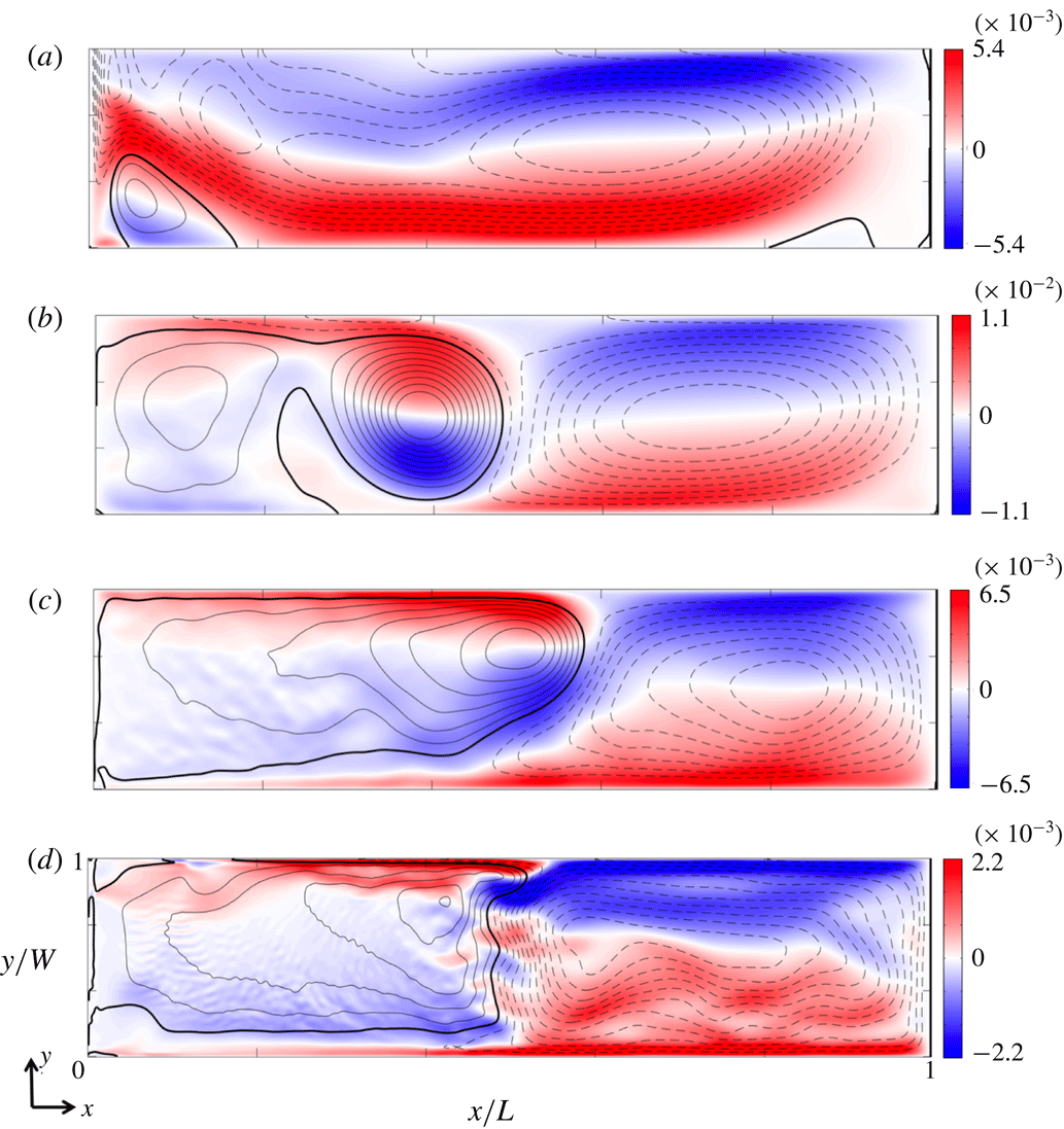
The dependence of the corresponding mid-depth horizontal circulation on rotation rate is shown in figure 6 by the
 $x$
component of the mean velocity and the corresponding horizontal transport
 $\unicode[STIX]{x1D713}_{H}$
at
 $z=H/2$
. The weakly rotating case is dominated by a domain-sized cyclonic gyre, with a small anticyclonic gyre near the endwall plume over the destabilising heated region. As rotation increases, a cyclonic gyre remains present over the stabilising half of the domain, while one or two anticyclonic gyres form over the heated region. At
 $Ro_{\unicode[STIX]{x0394}T}=3.6\times 10^{-3}$
the anticyclonic gyre centred at
 $\hat{x}=0.4$
is strong, but with increasing rotation the anticyclonic gyre over the destabilising region becomes relatively weak compared with the cyclonic gyre over the stabilising region.
Time-averaged horizontal flow at mid-depth over 600 buoyancy time scales for different Rossby numbers: colour scale shows normalised velocity in the
 $x$
direction,
 $u/\sqrt{g^{\prime }L}$
, on the plane
 $z/H=0.5$
; line contours show the normalised streamfunction
 $\unicode[STIX]{x1D713}_{H}/(L\sqrt{g^{\prime }L})$
computed at this height. The solutions are for
 $Ra=7.4\times 10^{11}$
and Rossby number (a)
 $Ro_{\unicode[STIX]{x0394}T}=1.6\times 10^{-1}$
(streamfunction increment
 $\unicode[STIX]{x0394}\unicode[STIX]{x1D713}_{H}/L\sqrt{g^{\prime }L}=3.1\times 10^{-5}$
), (b)
 $Ro_{\unicode[STIX]{x0394}T}=3.6\times 10^{-3}$
(
 $\unicode[STIX]{x0394}\unicode[STIX]{x1D713}_{H}/L\sqrt{g^{\prime }L}=5.2\times 10^{-5}$
), (c)
 $Ro_{\unicode[STIX]{x0394}T}=3.6\times 10^{-4}$
, no-slip (
 $\unicode[STIX]{x0394}\unicode[STIX]{x1D713}_{H}/L\sqrt{g^{\prime }L}=3.4\times 10^{-5}$
), and (d)
 $Ro_{\unicode[STIX]{x0394}T}=1.7\times 10^{-5}$
(
 $\unicode[STIX]{x0394}\unicode[STIX]{x1D713}_{H}/L\sqrt{g^{\prime }L}=1.0\times 10^{-5}$
). Black lines show clockwise (anticyclonic) circulation, thick black line is the zero contour, thin broken lines are anticlockwise and
 $g^{\prime }=g\unicode[STIX]{x1D6FC}\unicode[STIX]{x0394}T$
.

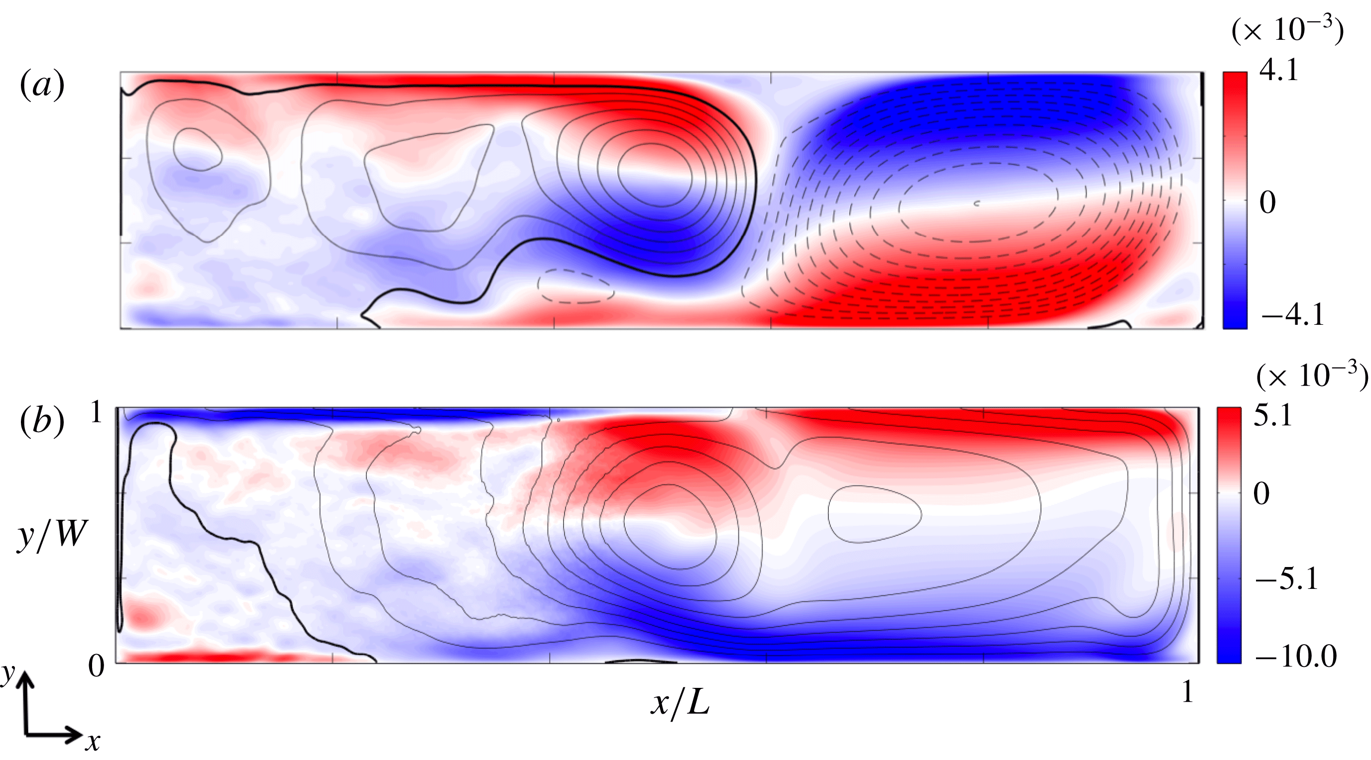
The boundary layer and mid-depth horizontal velocity and streamfunctions for the larger
 $Ra$
are shown in figure 7. The dynamics are similar to those at the smaller
 $Ra$
at similar
 $Ro_{\unicode[STIX]{x0394}T}$
(
 $Ro_{\unicode[STIX]{x0394}T}=3.6\times 10^{-3}$
and
 $Ro_{\unicode[STIX]{x0394}T}=3.6\times 10^{-4}$
). At mid-depth there is a strong cyclonic gyre over the stabilising region and anticyclonic flow over the destabilising region (figure 7
a). In the boundary layer an anticyclonic gyre dominates much of the flow, with remnants of a weak cyclonic gyre over the heated end of the domain near the endwall (figure 7
b). The structure of the mean flow is thus primarily dependent on Rossby number.
A comparison of time-averaged horizontal flow (over 65 buoyancy time scales) in the interior and boundary layer: colour scale shows normalised velocity in the
 $x$
direction,
 $u/\sqrt{g^{\prime }L}$
; line contours show the normalised streamfunction
 $\unicode[STIX]{x1D713}_{H}/(L\sqrt{g^{\prime }L})$
computed at this height. The solutions are for
 $Ra=7.4\times 10^{12}$
and Rossby number
 $Ro_{\unicode[STIX]{x0394}T}=1.1\times 10^{-3}$
on the plane (a) at mid-depth
 $z/H=0.5$
(streamfunction increment
 $\unicode[STIX]{x0394}\unicode[STIX]{x1D713}_{H}/L\sqrt{g^{\prime }L}=3.2\times 10^{-5}$
), and (b) in the boundary layer
 $z=\unicode[STIX]{x1D6FF}/2$
(
 $\unicode[STIX]{x0394}\unicode[STIX]{x1D713}_{H}/L\sqrt{g^{\prime }L}=6.6\times 10^{-5}$
). Black lines show clockwise (anticyclonic) circulation, thick black line is the zero contour, thin broken lines are anticlockwise and
 $g^{\prime }=g\unicode[STIX]{x1D6FC}\unicode[STIX]{x0394}T$
.

The mean overturning (vertical) circulation, shown in figure 8, is illustrated by zonal (
 $y$
) averages of the time-averaged
 $x$
component of velocity along with contours of the zonally integrated transport
 $\unicode[STIX]{x1D709}_{vert}$
(2.5). For weak rotation, the main upwelling leg of the circulation occurs near the endwall, whereas for strong rotation relative to weak buoyancy forcing (
 $Ro_{\unicode[STIX]{x0394}T}<10^{-1}$
) it shifts to a relatively wide area above the heated base, separated from the endwall. For the strongest rotation (
 $Ro_{\unicode[STIX]{x0394}T}=1.7\times 10^{-5}$
; figure 8
d) there is a relatively weak counter-rotating cell at
 $\hat{x}<0.25$
. Although this may appear to be a dramatic change in the mean overturning circulation, it is important to note that the flow is three-dimensional (including the upwelling near the walls) and the counter-rotating cell is likely to be an artefact of the zonal averaging. Rotation has less affect on the pattern of the overturning transport above the cooled region of the base. The solution for the larger value of the Rayleigh number (
 $Ra=7.4\times 10^{12}$
) shows overturning similar in pattern and magnitude to that in figure 8(b) over the heated region and a similar pattern but smaller strength compared to figure 8(c) over the cooled region. In addition to the mean overturning transport (2.5) shown in figure 8 we also calculate the ‘residual mean circulation’ in appendix A, but find that, in the present case for flow in a closed box and driven solely by buoyancy, it does not reveal any new information about the flow.
Time-averaged and zonally averaged velocity in the
 $x$
direction,
 $u/\sqrt{g^{\prime }L}$
, projected on a vertical plane (colour contours) and zonally integrated mean overturning transport
 $\unicode[STIX]{x1D709}_{vert}/L^{2}\sqrt{g^{\prime }L}$
(line contours) for
 $Ra=7.4\times 10^{11}$
and Rossby number (a)
 $Ro_{\unicode[STIX]{x0394}T}=1.6\times 10^{-1}$
(transport increment
 $\unicode[STIX]{x0394}\unicode[STIX]{x1D709}_{vert}/L^{2}\sqrt{g^{\prime }L}=5.0\times 10^{-6}$
), (b)
 $Ro_{\unicode[STIX]{x0394}T}=3.6\times 10^{-3}$
(
 $\unicode[STIX]{x0394}\unicode[STIX]{x1D709}_{vert}/L^{2}\sqrt{g^{\prime }L}=2.5\times 10^{-6}$
), (c)
 $Ro_{\unicode[STIX]{x0394}T}=3.6\times 10^{-4}$
, no-slip (
 $\unicode[STIX]{x0394}\unicode[STIX]{x1D709}_{vert}/L^{2}\sqrt{g^{\prime }L}=1.2\times 10^{-6}$
), and (d)
 $Ro_{\unicode[STIX]{x0394}T}=1.7\times 10^{-5}$
(
 $\unicode[STIX]{x0394}\unicode[STIX]{x1D709}_{vert}/L^{2}\sqrt{g^{\prime }L}=5.0\times 10^{-7}$
). Time averaging is over 600 buoyancy time scales. Thin black lines show clockwise overturning, thick black line is the zero contour, thin broken lines are anticlockwise and
 $g^{\prime }=g\unicode[STIX]{x1D6FC}\unicode[STIX]{x0394}T$
.

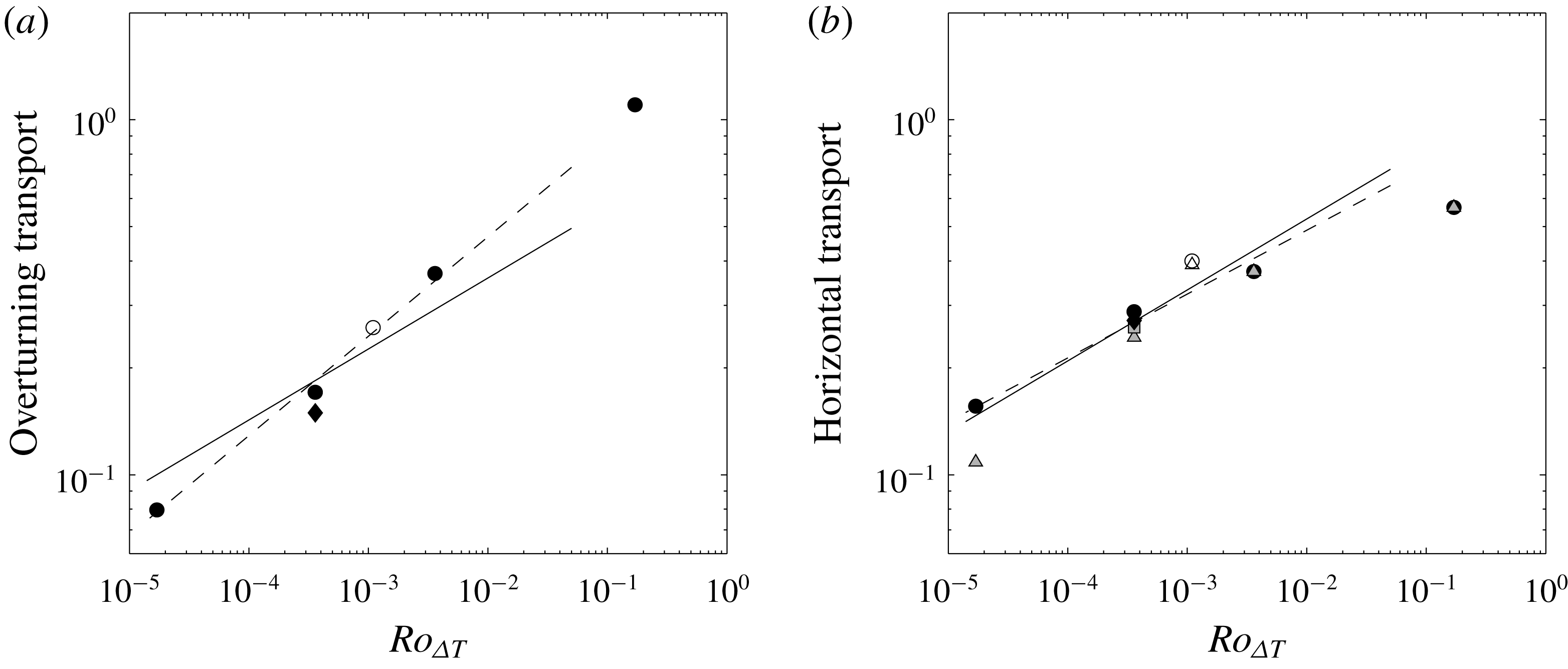
The dependence of the mean circulation on governing parameters can be summarised by the maximum values of the integrated transports
 $\unicode[STIX]{x1D709}_{H}$
and
 $\unicode[STIX]{x1D709}_{vert}$
defined in (2.6) and (2.5), respectively, and plotted in figure 9. Also shown is the maximum value of the baroclinic component of the horizontal transport in the boundary layer
 $\unicode[STIX]{x1D709}_{B}$
defined in (2.7). All transport values in figure 9 are normalised by the established scaling (2.8) for the overturning transport in the inertial boundary layer regime of the non-rotating, large-Rayleigh-number case. The results show that all measures of the transport decrease with decreasing Rossby number. The barotropic contribution to the total horizontal transport in the boundary layer is small and insignificant in all cases except at the smallest Rossby number, where the barotropic component reduces the total boundary layer transport by
 ${\sim}30\,\%$
of the baroclinic transport. Hence this convectively driven geostrophic circulation can develop a significant barotropic component despite zero net momentum input. The total horizontal boundary layer transport (at least as measured by the transport maximum) is less than the maximum in the baroclinic contribution due to differences in the sign of the horizontal streamfunctions in the interior and boundary layer over significant areas of the basin.
Maximum values of (a) the overturning transport and (b) the total horizontal transport in the boundary layer
 $\unicode[STIX]{x1D709}_{H}$
(circles, no-slip; diamond, free-slip) and its baroclinic component
 $\unicode[STIX]{x1D709}_{B}$
(triangles, no-slip; square, free-slip). All transports are normalised by the non-rotating scaling for the overturning (2.8) (with constant
 $c_{0}=1$
) for
 $Ra=7.4\times 10^{11}$
(filled symbols). Points at
 $Ro_{\unicode[STIX]{x0394}T}=1.1\times 10^{-3}$
are for large Rayleigh number
 $Ra=7.4\times 10^{12}$
(open symbols). The solid line is the geostrophic–diffusive boundary layer scaling prediction (2.10)
 $\unicode[STIX]{x1D709}/\unicode[STIX]{x1D709}_{0}=c_{1}Ro_{\unicode[STIX]{x0394}T}^{1/5}$
fitted to no-slip
 $Ra=7.4\times 10^{11}$
results (filled circles) for
 $Ro_{\unicode[STIX]{x0394}T}\leqslant 0.05$
with prefactor value (a)
 $c_{1}=1.1$
for
 $\unicode[STIX]{x1D709}_{vert}$
and (b)
 $c_{1}=1.3$
for
 $\unicode[STIX]{x1D709}_{B}$
. Broken lines are best-fitting power laws to no-slip
 $Ra=7.4\times 10^{11}$
results (filled circles) for (a)
 $\unicode[STIX]{x1D709}_{vert}/\unicode[STIX]{x1D709}_{0}=1.7Ro_{\unicode[STIX]{x0394}T}^{0.28}$
and (b)
 $\unicode[STIX]{x1D709}_{B}/\unicode[STIX]{x1D709}_{0}=1.1Ro_{\unicode[STIX]{x0394}T}^{0.18}$
. The overturning transport at
 $Ro_{\unicode[STIX]{x0394}T}=0.16$
is greater than that for the non-rotating case due to Ekman transport.

The computed transport in figure 9 can be compared with the geostrophic scaling predictions. The scaling for the geostrophic regime (2.9) predicts that the two streamfunctions will have different dependence on rotation rate, whereas the integrated overturning transport (2.10) (hence the net boundary layer transport in the
 $x$
direction) will be in fixed proportional to the depth-integrated baroclinic horizontal transport in the recirculating gyres. The results in figure 9 indicate instead that the total boundary layer transport
 $\unicode[STIX]{x1D709}_{H}$
trends like the overturning transport
 $\unicode[STIX]{x1D709}_{vert}$
, whereas only the baroclinic contribution to the boundary layer transport trends close to the predicted thermal wind scaling
 $Ro_{\unicode[STIX]{x0394}T}^{1/5}$
. The baroclinic boundary layer transport is larger than the overturning at
 $Ro_{\unicode[STIX]{x0394}T}<10^{-2}$
. We conclude that both the vertical overturning and total horizontal transports are more strongly inhibited at strong rotation than is the horizontal baroclinic component of the flow in the boundary layer. Since the time-averaged flow is approximately geostrophic, the baroclinic component is essentially the thermal wind. The results also show little difference in the computed transports between the cases of free-slip sidewall and no-slip sidewall boundary conditions. The success of the geostrophic scaling in predicting the horizontal transport provides evidence that the circulation is governed by a vertical advection–diffusion balance (above the region of stabilising boundary heat flux) together with a geostrophic balance in the basin-scale flow of the boundary layer, and that the interior dynamics play a lesser role.
5 Heat transport
5.1 Heat transport diagnostics
Given that all scales of flow and diffusion are resolved in the present simulations and the surface boundary conditions are imposed temperatures, the heat flux at the base is diffusive and the total heat transported through the system is the integrated flux through the area of positive boundary flux. The use of an almost piecewise-uniform distribution of the imposed boundary temperatures leads to no significant differences between the area of positive boundary flux from the area of imposed higher temperature
 $T_{h}$
. The total heat throughput is therefore
 $(\unicode[STIX]{x1D70C}_{r}c_{p})^{-1}FA_{hot}=\unicode[STIX]{x1D705}\int _{A_{hot}}\overline{(\unicode[STIX]{x2202}T/\unicode[STIX]{x2202}z)}\,\text{d}a$
, where the area of the heated base is
 $A_{hot}\approx WL/2$
and the overbar indicates a time average. The Nusselt number is evaluated as
 $Nu=2\int _{A_{hot}}\overline{(\unicode[STIX]{x2202}T/\unicode[STIX]{x2202}z)}\,\text{d}a/(\unicode[STIX]{x0394}TW)$
.
For the values of
 $Ra$
considered here, the boundary layer on the cool region of the base is laminar. Downwelling flow of warmer water from the interior into the boundary layer leads to a balance of advection and vertical diffusion of heat. Above the heated region of the base, the average temperature gradient at the boundary must be equal to but of opposite sign from that at the cold boundary, so that there is no net heat input to the box. However, this causes much of the thermal boundary layer on the heated region to be unstable, and a mixed layer of small-scale turbulent convection forms between a very thin diffusive sublayer on the boundary and an overlying stably stratified portion of the boundary layer flow (Mullarney et al.
Reference Mullarney, Griffiths and Hughes2004). The convective circulation also includes plumes in the interior and near the side boundaries above the heated half of the base, carrying water and heat from the boundary layer into the interior.
The mechanisms responsible for heat transport can be examined further by distinguishing the contributions to heat transport by the time mean and fluctuating components of flow in local regions within the basin. Focusing particularly on the vertical transport, the vertical velocity
 $w=\overline{w}+w^{\prime }$
and temperature field
 $T=\overline{T}+T^{\prime }$
imply heat transfer
 $Q_{h}$
across a horizontal plane of horizontal area
 $a$
at a rate
 $$\begin{eqnarray}(\unicode[STIX]{x1D70C}_{r}c_{p})^{-1}Q_{h}=\int \overline{wT}\,\text{d}a-\unicode[STIX]{x1D705}\int \overline{(\unicode[STIX]{x2202}T/\unicode[STIX]{x2202}z)}\,\text{d}a,\end{eqnarray}$$
and this can be expressed in terms of the mean and fluctuating contributions as
 $$\begin{eqnarray}(\unicode[STIX]{x1D70C}_{r}c_{p})^{-1}Q_{h}-\overline{T}_{ref}\int \overline{w}\,\text{d}a=\int \overline{w}(\overline{T}-\overline{T}_{ref})\,\text{d}a+\int \overline{w^{\prime }T^{\prime }}\,\text{d}a-\unicode[STIX]{x1D705}\int \overline{(\unicode[STIX]{x2202}T/\unicode[STIX]{x2202}z)}\,\text{d}a,\end{eqnarray}$$
where the reference temperature
 $\overline{T}_{ref}$
is introduced in order to remove the large and irrelevant transport of heat by mean flow having a non-zero absolute temperature. The mean and fluctuation contributions of advective transport on the right of (5.2) will be examined for the full area of the basin, but also in subregions chosen to encompass the side boundary processes, the interior vertical convection, or the heated and cooled halves. The reference temperature
 $\overline{T}_{ref}={\mathcal{A}}^{-1}\int _{{\mathcal{A}}}T\,\text{d}a$
was chosen as the horizontally averaged temperature over the full area
 ${\mathcal{A}}=LW$
of the basin on the horizontal plane of interest. Hence the temperature anomaly
 $T^{\ast }=T-T_{ref}$
is such that positive heat transport is either by upwelling of water that is relatively warm compared to the average temperature over the whole area of the basin at the same level, or by downwelling of water that is relatively cool for that level. When integrating over the full area of the basin, the net advection at the reference temperature on the left of (5.2) vanishes (by continuity
 $\int _{{\mathcal{A}}}\overline{w}\,\text{d}a=0$
). When considering a time average of the thermal equilibrium state and integrating over the full area, there must also be zero net heat transport across any horizontal level in the fluid (
 $\int _{{\mathcal{A}}}\overline{wT}\,\text{d}a=\unicode[STIX]{x1D705}\int _{{\mathcal{A}}}\overline{(\unicode[STIX]{x2202}T/\unicode[STIX]{x2202}z)}\,\text{d}a$
).
5.2 Contributions to heat transport
The overall heat transport through the basin was reported for the lower-Rayleigh-number cases in Vreugdenhil et al. (Reference Vreugdenhil, Gayen and Griffiths2016) and the Nusselt-number values are repeated in table 1. Those values, along with that for the new solution at the higher Rayleigh number, are consistent with both the
 $Ra$
and
 $Ro_{\unicode[STIX]{x0394}T}$
dependence predicted by the geostrophic scaling (2.4). Here we examine the vertical transport of heat into the interior and the mechanisms responsible.
Snapshots of vertical velocity, temperature and the vertical advective heat flux at mid-depth (
 $\hat{z}=0.5$
) are shown in figure 10 for the higher Rayleigh number
 $Ra=7.4\times 10^{12}$
and
 $Ro_{\unicode[STIX]{x0394}T}=1.1\times 10^{-3}$
. The mid-depth plane is chosen here in order to remain clear of the spatially and temporally varying thermal boundary layer thickness, particularly at the strongest rotation rate. Results for the smaller
 $Ra$
at
 $Ro_{\unicode[STIX]{x0394}T}<10^{-1}$
are similar, including the case having free-slip sidewalls. Upwelling velocities are largest in the warm vortical plumes, which are distributed through the region
 $\hat{x}<0.3$
(figure 10
a,b). These plumes are generally surrounded by significantly slower downward motion of water that is cooler than the plumes but warmer than the basin-wide average
 $\overline{T}_{ref}$
on this plane, hence contributing downward heat flux.
Snapshots at mid-depth (
 $\hat{z}=0.5$
) for
 $Ra=7.4\times 10^{12}$
,
 $Ro_{\unicode[STIX]{x0394}T}=1.1\times 10^{-3}$
: (a) normalised vertical velocity
 $w/\sqrt{g\unicode[STIX]{x1D6FC}\unicode[STIX]{x0394}TL}$
; (b) normalised temperature
 $\hat{T}$
; and (c) normalised advective heat flux (per unit area)
 $wT^{\ast }/\unicode[STIX]{x1D705}\overline{(\unicode[STIX]{x2202}T/\unicode[STIX]{x2202}z)}_{hot}$
through the horizontal plane, where
 $\unicode[STIX]{x1D705}\overline{(\unicode[STIX]{x2202}T/\unicode[STIX]{x2202}z)}_{hot}$
is the average input heat flux (per unit area) from the warm half of the base.

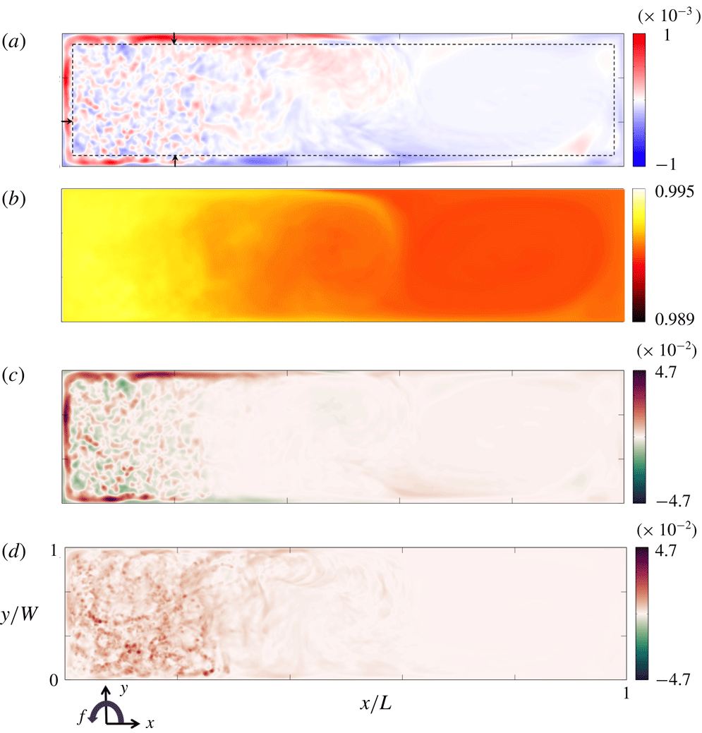
The corresponding time-averaged quantities (vertical velocity, temperature and advective vertical heat flux) on the mid-depth plane (figure 11) reveal a substantial role of the side boundaries. There is mean upwelling of warm water at the three walls bounding the destabilised half of the basin. There is only a very small mean vertical volume flux in the interior region of deep columnar convection, and it is in the opposite direction. For the case shown in figure 11(a), the average vertical velocity over the area outside the boundary plumes and at
 $\hat{x}<0.3$
, at mid-depth, is just
 $-0.3\,\%$
(i.e. downwards) of the maximum time-averaged velocity in the side boundary plumes. The width of this sidewall upwelling, plotted in figure 12, was estimated by measuring the distance from the wall at which the vertical velocity is 10 % of the maximum mean vertical velocity, at three chosen locations (shown in figure 11) and averaging these. For weak rotation (
 $Ro_{\unicode[STIX]{x0394}T}=0.16$
) there was no distinct upwelling on the ‘eastern’ and ‘western’ boundaries, and in place of this the width of the endwall plume is plotted for this case. The width of boundary upwelling decreases with increasing rotation, with a best-fitting power law
 $Ro_{\unicode[STIX]{x0394}T}^{1/3}\sim f^{-5/9}$
: this dependence is significantly stronger than that predicted for viscous Stewartson layers (
 $f^{-1/4}$
) but significantly weaker than in a scaling with the Rossby deformation radius, as has previously been suggested (Spall Reference Spall2011; Cenedese Reference Cenedese2012). An important result is that similar side boundary upwelling zones also occur in the case of free-slip sidewalls, where they are only 20 % narrower (filled triangle in figure 12). Hence the upwelling is not a viscous boundary layer phenomenon and is instead buoyancy-driven, stationary line plumes at the boundaries. As they are driven by gravitationally unstable temperature differences, the width of the plumes is not directly related to the deformation radius based on the overall density difference and that characterises the stable density stratification elsewhere in the circulation.
Time-averaged quantities at mid-depth (
 $\hat{z}=0.5$
) corresponding to figure 10, for an averaging period 65
 $\unicode[STIX]{x1D70F}_{b}$
: (a) mean vertical velocity
 $\overline{w}/\sqrt{g\unicode[STIX]{x1D6FC}\unicode[STIX]{x0394}TL}$
; (b) mean temperature
 $\overline{\hat{T}}$
; and (c,d) time-averaged advective heat flux (per unit area) through the plane by, respectively, the mean
 $\overline{w}\overline{T^{\ast }}/\unicode[STIX]{x1D705}\overline{(\unicode[STIX]{x2202}T/\unicode[STIX]{x2202}z)}_{hot}$
and fluctuating
 $\overline{{w^{\prime }T}^{\prime }}/\unicode[STIX]{x1D705}\overline{(\unicode[STIX]{x2202}T/\unicode[STIX]{x2202}z)}_{hot}$
components of the flow. Heat fluxes are normalised by
 $\unicode[STIX]{x1D705}\overline{(\unicode[STIX]{x2202}T/\unicode[STIX]{x2202}z)}_{hot}$
, the time- and area-averaged heat flux (per unit area) into the basin from the heated area of the base. In (a) the arrows show the locations where the width of the boundary upwelling zone is measured, and the broken line is the average of the three measured widths.

Width of the side boundary upwelling zones relative to basin length
 $L$
as a function of Rossby number for
 $Ra=7.4\times 10^{11}$
(closed symbols, triangle for no-slip sidewalls) and
 $Ra=7.4\times 10^{12}$
(open square). The broken line indicates theoretical Stewartson layer thickness
 $\unicode[STIX]{x1D6FF}_{S}/L=(2E)^{1/4}\sim Ro_{\unicode[STIX]{x0394}T}^{3/20}$
; solid line is the best fit (
 $0.22Ro_{\unicode[STIX]{x0394}T}^{1/3}$
) for
 $Ra=7.4\times 10^{11}$
,
 $Ro_{\unicode[STIX]{x0394}T}<10^{-1}$
(no-slip sidewalls).

Advective heat flux due to the mean flow,
 $\overline{w}\overline{T^{\ast }}$
(figure 11
c), reflects the mean vertical velocities and is largest in the side boundary upwelling zones. It is positive also through the bulk of the cooled half of the basin (corresponding to a slow downward motion of water cooler than
 $\overline{T}_{ref}$
), where it approximately balances the mean downward diffusion of heat in the mean temperature gradient. In contrast, the contribution of the fluctuating (plume) component of flow,
 $\overline{w^{\prime }T^{\prime }}$
(figure 11
d), carries heat upwards in much of the interior at
 $\hat{x}<0.3$
. The averaging period of
 $65\unicode[STIX]{x1D70F}_{b}$
(which for the case in figure 11 equates to 1600 rotation periods) does not completely remove the signature of the interior vortical plumes, as these are long-lived, slowly migrating structures. The solution for
 $Ra=7.4\times 10^{11},~Ro_{\unicode[STIX]{x0394}T}=3.6\times 10^{-3}$
(not shown) has an additional weak downward transport of heat by fluctuations inside a large anticyclonic gyre near
 $\hat{x}=0.6$
.
Time-averaged heat transport contributions through the horizontal mid-depth plane
 $z=H/2$
, plotted as a function of Rossby number, carried by the fluctuating component of flow
 $\int _{{\mathcal{A}}}\overline{w^{\prime }T^{\prime }}\,\text{d}a$
(red triangles; as shown in figure 11
d) and by the mean flow
 $\int \overline{w}\overline{T^{\ast }}\,\text{d}a$
(as shown in figure 11
c), where the latter is separated into contributions from horizontal sub-areas
 $a$
in the interior (blue circles) and sidewall upwelling zones (cyan circles):
 $Ra=7.4\times 10^{11}$
(solid symbols, no-slip sidewall results linked by the broken lines; free-slip wall results are those lying slightly off the lines at
 $Ro_{\unicode[STIX]{x0394}T}=4\times 10^{-4}$
);
 $Ra=7.4\times 10^{12}$
(open symbol). The inset shows the total mean diffusive component of vertical heat transport
 $\unicode[STIX]{x1D705}\int _{{\mathcal{A}}}\unicode[STIX]{x2202}\overline{T}/\unicode[STIX]{x2202}z\,\text{d}a$
at mid-depth. Heat transports are normalised by the total heat throughput
 $\unicode[STIX]{x1D705}\int _{A_{hot}}\overline{(\unicode[STIX]{x2202}T/\unicode[STIX]{x2202}z)}|_{z=0}\,\text{d}a$
and are averaged over 600
 $\unicode[STIX]{x1D70F}_{b}$
for
 $Ra=7.4\times 10^{11}$
and 65
 $\unicode[STIX]{x1D70F}_{b}$
for
 $Ra=7.4\times 10^{12}$
.

Area-integrated contributions to mean vertical heat transport through the mid-depth plane in subregions of the basin are compared in figure 13. Shown here are the mean flow contributions in the subregions encompassing either the side boundary upwelling zones or the interior above the heated half of the base, along with the heat transport by fluctuations over the whole basin area (which is not spatially decomposed, as the fluctuations are overwhelmingly the plumes in the interior region of chimney convection). Similarly the heat transport by diffusion (inset in figure 13) is shown only for the whole basin area. The diffusive transport in all cases transports heat downwards as a result of the stable mean temperature gradient: it is very small for
 $Ro_{\unicode[STIX]{x0394}T}>10^{-1}$
(as in the non-rotating case), increases with increasing rotation (reflecting increased stratification in the interior; figure 2), and is notably larger for the smallest Rossby number. The total of all contributions sum to zero net heat transport through the plane. All contributions at this level are small compared to the total heat throughput (which is used to normalise each contribution in figure 13), as most of the throughput is carried horizontally by flow in the thermal boundary layer.
The vertical heat transport by the mean flow does not trend systematically at moderate Rossby numbers. However, it is positive in the sidewall upwelling zones and negative in the interior. At
 $Ro_{\unicode[STIX]{x0394}T}=3.6\times 10^{-3}$
these two contributions are comparable, implying that the vertical heat transport is largely by a coherent zonal mean overturning, which we associate with a strong anticyclonic gyre near the centre of the basin, present only in this run. At stronger rotation (
 $Ro_{\unicode[STIX]{x0394}T}<10^{-3}$
) interior transport by mean flow becomes negligible, the mean sidewall upwelling and interior fluctuating flow give comparable (and positive) contributions, and the total mean heat transport is balanced by the mean downward diffusion of heat, the latter becoming the largest term at extreme rotation. The heat transport by fluctuating flow is downward at weak rotation, where it is confined to the endwall plume in which
 $\text{d}\overline{T}/\text{d}z<0$
, and changes sign at
 $Ro_{\unicode[STIX]{x0394}T}\approx 10^{-2}$
. At Rossby numbers less than this, the chimney convection in the interior takes place within the positive mean temperature gradient. The fluctuating flow, representing the vortical plumes, gives an increasingly large upward heat transport with increasing rotation, becoming the second largest contribution (after mean diffusion) at extreme rotation due to a larger number of vortical plumes.
6 Mechanical energy budget
6.1 Energy budget diagnostics
The energy source for the flow is the generation of available potential energy (APE) by the boundary buoyancy forcing. The APE is converted (by the reversible buoyancy flux, integrated over the full volume
 ${\mathcal{V}}$
of the basin) to kinetic energy at a matching rate
 $\unicode[STIX]{x1D6F7}_{z}=g\int _{{\mathcal{V}}}w\unicode[STIX]{x1D70C}\,\text{d}V$
(Winters et al.
Reference Winters, Lombard, Riley and D’Asaro1995; Hughes, Hogg & Griffiths Reference Hughes, Hogg and Griffiths2009). This energy transfer can be decomposed into contributions from the time-averaged and fluctuating components of the flow,
 $\overline{\unicode[STIX]{x1D6F7}_{z}}=g\int _{{\mathcal{V}}}\overline{w}\bar{\unicode[STIX]{x1D70C}}\,\text{d}V$
and
 ${\unicode[STIX]{x1D6F7}_{z}}^{\prime }=g\int _{{\mathcal{V}}}\overline{w^{\prime }\unicode[STIX]{x1D70C}^{\prime }}\,\text{d}V$
, respectively, corresponding to large-scale circulation and small-scale convection (Gayen et al.
Reference Gayen, Griffiths, Hughes and Saenz2013, Reference Gayen, Griffiths and Hughes2014). The roles of these contributions have not previously been examined for geostrophic circulation with resolved convection. The roles of these contributions in the case of non-rotating convection have been discussed in an alternative framework of a locally defined APE density (Scotti & White Reference Scotti and White2014). In the present study we choose to use the APE framework of Winters et al. (Reference Winters, Lombard, Riley and D’Asaro1995) and Hughes et al. (Reference Hughes, Hogg and Griffiths2009), with energy conversions computed from the mean and fluctuating parts of the velocity and buoyancy fluxes, an approach that is widely familiar in fluid dynamics.
There are two sinks in the mechanical energy budget: viscous dissipation and mixing of density (Winters et al.
Reference Winters, Lombard, Riley and D’Asaro1995; Peltier & Caulfield Reference Peltier and Caulfield2003; Hughes et al.
Reference Hughes, Hogg and Griffiths2009). Viscous dissipation converts kinetic energy into internal energy. The rate of viscous dissipation
 $\unicode[STIX]{x1D700}$
in a volume of interest
 $V$
is
 $\unicode[STIX]{x1D700}=\unicode[STIX]{x1D70C}_{r}\unicode[STIX]{x1D708}\int (\unicode[STIX]{x2202}u_{i}/\unicode[STIX]{x2202}x_{j})^{2}\,\text{d}V$
, where
 $u_{i}$
are components of the velocity,
 $x_{i}$
are displacements, the subscripts
 $i$
and
 $j$
are orthogonal directions and summation is implied. In the time-averaged thermally equilibrated state, the present simulations confirm that the total rates of generation and dissipation of kinetic energy (
 $\unicode[STIX]{x1D700}_{T}$
when integrated over the whole volume of the basin) are accurately matched. They also match the net production of potential energy,
 $$\begin{eqnarray}\unicode[STIX]{x1D6F7}_{i}=-g\unicode[STIX]{x1D705}WL(\langle \unicode[STIX]{x1D70C}\rangle _{H}-\langle \unicode[STIX]{x1D70C}\rangle _{0}),\end{eqnarray}$$
which is due only to diffusion of heat down the small mean top-to-bottom vertical temperature gradient (
 $\langle \unicode[STIX]{x1D70C}\rangle _{H}$
and
 $\langle \unicode[STIX]{x1D70C}\rangle _{0}$
being the horizontally averaged densities at the top and bottom boundaries, respectively (Paparella & Young Reference Paparella and Young2002; Hughes et al.
Reference Hughes, Hogg and Griffiths2009; Vreugdenhil et al.
Reference Vreugdenhil, Gayen and Griffiths2016)). That is,
 $\unicode[STIX]{x1D700}_{T}=\unicode[STIX]{x1D6F7}_{i}$
. The results further imply that the rate of viscous dissipation, in the turbulent boundary layer regime, is approximately independent of rotation, and that any weak dependence is a consequence of a rotation-dependent top-to-bottom density difference.
The second energy sink is conversion of APE due to the mixing of the density field. The rate of mixing in any subvolume
 $V$
is given by
 $\unicode[STIX]{x1D6F7}_{d}=-g\unicode[STIX]{x1D705}\int (\text{d}z^{\ast }/\text{d}\unicode[STIX]{x1D70C})(\unicode[STIX]{x2202}\unicode[STIX]{x1D70C}/\unicode[STIX]{x2202}x_{i})^{2}\,\text{d}V$
, where
 $z^{\ast }$
is the height of the water parcel (above the base) if all the water parcels in the basin were adiabatically reordered into the rest state of gravitational equilibrium (Hughes et al.
Reference Hughes, Hogg and Griffiths2009). Energetics frameworks for incompressible fluids under the Boussinesq approximation and with a linear equation of state describe the role of this mixing as an irreversible transfer of APE to background potential energy (Winters et al.
Reference Winters, Lombard, Riley and D’Asaro1995; Peltier & Caulfield Reference Peltier and Caulfield2003; Hughes et al.
Reference Hughes, Hogg and Griffiths2009). (For a nonlinear equation of state or a compressible fluid, a more complete description is required, in which the changes in APE and background potential energy are not equal and the APE is irreversibly converted to internal energy, hence a contribution to Joule heating (Tailleux Reference Tailleux2009, Reference Tailleux2013, Reference Tailleux2018).) For the Boussinesq fluid with a linear equation of state considered here, in a time-averaged thermally equilibrated state, the mixing rate
 $\unicode[STIX]{x1D6F7}_{d}$
integrated over the whole volume of the basin must equal the rate of generation of APE by buoyancy forcing at the boundary (Hughes et al.
Reference Hughes, Hogg and Griffiths2009; Tailleux Reference Tailleux2009; Gayen et al.
Reference Gayen, Griffiths, Hughes and Saenz2013, Reference Gayen, Griffiths and Hughes2014). A previous theoretical result (Gayen et al.
Reference Gayen, Griffiths, Hughes and Saenz2013), confirmed by DNS (Gayen et al.
Reference Gayen, Griffiths and Hughes2014), is that the mixing rate is related simply to the heat transport in a manner that is independent of rotation (
 $\unicode[STIX]{x1D6F7}_{d}/\unicode[STIX]{x1D700}_{T}\sim NuA_{x}$
) and this can be re-expressed in terms of the Rossby number defined here:
 $$\begin{eqnarray}\unicode[STIX]{x1D6F7}_{d}/\unicode[STIX]{x1D700}_{T}\sim (RaPrRo_{\unicode[STIX]{x0394}T})^{1/5}.\end{eqnarray}$$
The energy conversions outlined above can be used to define a global mixing efficiency
 $$\begin{eqnarray}\unicode[STIX]{x1D702}=\frac{\unicode[STIX]{x1D6F7}_{d}-\unicode[STIX]{x1D6F7}_{i}}{\unicode[STIX]{x1D6F7}_{d}-\unicode[STIX]{x1D6F7}_{i}+\unicode[STIX]{x1D700}_{T}}\end{eqnarray}$$
(Peltier & Caulfield Reference Peltier and Caulfield2003; Hughes et al.
Reference Hughes, Hogg and Griffiths2009). Applying the steady-state result that
 $\unicode[STIX]{x1D700}_{T}=\unicode[STIX]{x1D6F7}_{i}$
, the mixing efficiency becomes
 $$\begin{eqnarray}\unicode[STIX]{x1D702}=1-\frac{\unicode[STIX]{x1D700}_{T}}{\unicode[STIX]{x1D6F7}_{d}}.\end{eqnarray}$$
The scaling above (
 $\unicode[STIX]{x1D6F7}_{d}/\unicode[STIX]{x1D700}_{T}\sim NuA_{x}$
) coupled with (2.10) then gives (Gayen et al.
Reference Gayen, Griffiths, Hughes and Saenz2013)
 $$\begin{eqnarray}\unicode[STIX]{x1D702}\approx 1-(NuA_{x})^{-1}.\end{eqnarray}$$
The efficiency will therefore be smaller for larger rotation rates.
Whereas the global mixing efficiency helps to reveal the overall energy balances of the system, further insights can be obtained from the distribution of energy sinks in the flow and a local mixing efficiency. In order to define a local mixing efficiency, we recognise that
 $\unicode[STIX]{x1D6F7}_{i}$
is only defined as a global value, and use the result that at large Rayleigh numbers
 $\unicode[STIX]{x1D6F7}_{d}\gg \unicode[STIX]{x1D6F7}_{i}$
. A useful definition for a local mixing efficiency is then
 $\unicode[STIX]{x1D702}_{l}=\unicode[STIX]{x1D6F7}_{dl}/(\unicode[STIX]{x1D6F7}_{dl}+\unicode[STIX]{x1D700})$
, where
 $\unicode[STIX]{x1D6F7}_{dl}$
and
 $\unicode[STIX]{x1D700}$
are local (grid-scale) values of the mixing rate and viscous dissipation (Sohail, Gayen & Hogg Reference Sohail, Gayen and Hogg2018).
Snapshots of (a,b) viscous dissipation, (c,d) mixing rates (per unit volume), and (e,f) local mixing efficiency for
 $Ra=7.4\times 10^{12}$
,
 $Ro_{\unicode[STIX]{x0394}T}=1.1\times 10^{-3}$
. Panels (a,c,e) show zonally averaged quantities and (b,d,e) show quantities at a single depth of
 $\hat{z}=0.0055$
(within the thermal boundary layer, just outside of the Ekman layer). The dissipation and mixing are normalised by
 $\unicode[STIX]{x1D6F7}_{i}/HWL$
, where
 $\unicode[STIX]{x1D6F7}_{i}~(=\unicode[STIX]{x1D700}_{T})$
is from (6.1). The colour scale is logarithmic for dissipation and mixing.

The DNS for the smaller of the two Rayleigh-number values used here (Vreugdenhil et al. Reference Vreugdenhil, Gayen and Griffiths2016) showed the turbulent boundary layer regime and confirmed the behaviour predicted by (6.1)–(6.5). The basin-integrated mixing of density is smaller for larger rotation rates (as a result of increased boundary layer thickness and decreased buoyancy throughput), while the turbulent dissipation is unaffected by rotation. Thus the global mixing efficiencies are large (listed in table 1). In this paper we revisit the two energy sinks and discuss their spatial distribution.
6.2 Buoyancy flux, dissipation and mixing
The solutions can be interrogated to find the distributions of dissipation
 $\unicode[STIX]{x1D700}$
, mixing of density
 $\unicode[STIX]{x1D6F7}_{d}$
and the local mixing efficiency
 $\unicode[STIX]{x1D702}_{l}$
. The zonally averaged values and those on a plane at
 $\hat{z}=0.0055$
, just outside the Ekman layer, are shown in figure 14 for the case
 $Ra=7.4\times 10^{12}$
and
 $Ro_{\unicode[STIX]{x0394}T}=1.1\times 10^{-3}$
, where the rates of energy conversion are normalised by
 $\unicode[STIX]{x1D6F7}_{i}/HWL$
, the volume average rate of production of potential energy. The viscous dissipation is elevated at the base of the domain over the heated region (figure 14
a) and is especially large near the mid-section of the basin, where it is associated with combined small-scale convection and shear in the strong mean flow of the boundary layer current across the basin width and along the ‘eastern’ boundary (figure 14
b). Modest dissipation rates also appear in isolated patches beneath the vortical plumes. The mixing rate is strongest at the base, especially over the cooled region where the vertical temperature gradient is largest (figure 14
c). In the boundary layer, the largest mixing rates are around the edge of the convection chimney (the dark region in figure 14
d). Otherwise the mixing is distributed across the heated base and in the very small scales of convection. There is little mixing in the core of the chimney region at or above the height of the plane shown. At this height the two sinks are of comparable magnitude (figure 14
b,d). However, when summed over the volume of the basin, the mixing rate is an order of magnitude greater than the total dissipation rate, with the main site of mixing closer to the boundary than the plane chosen for figure 14(d). The local mixing efficiency shows values close to unity above the cooled region (figure 14
e) and at the edge of the convective chimney region (figure 14
f). When zonally averaged, most of the interior is at small to moderate local mixing efficiency. The columnar plumes through the depth appear as local highs in the interior dissipation, mixing and mixing efficiency, even in the zonal averages.
Distribution of dissipation
 $\unicode[STIX]{x1D700}$
for
 $Ra=7.4\times 10^{11}$
runs with (a)
 $Ro_{\unicode[STIX]{x0394}T}=1.6\times 10^{-1}$
, (b)
 $Ro_{\unicode[STIX]{x0394}T}=3.6\times 10^{-3}$
, (c)
 $Ro_{\unicode[STIX]{x0394}T}=3.6\times 10^{-4}$
and (d)
 $Ro_{\unicode[STIX]{x0394}T}=1.7\times 10^{-5}$
. Horizontal planes are taken within the boundary layer at (a)
 $\unicode[STIX]{x1D6FF}/H=0.011$
, (b)
 $\unicode[STIX]{x1D6FF}/H=0.011$
, (c)
 $\unicode[STIX]{x1D6FF}/H=0.006$
and (d)
 $\unicode[STIX]{x1D6FF}/H=0.0027$
. Excepting the weak rotation case (a), each plane is taken just outside the Ekman layer. The dissipation is normalised by
 $\unicode[STIX]{x1D6F7}_{i}/HWL$
.

Distribution of mixing
 $\unicode[STIX]{x1D6F7}_{d}$
for
 $Ra=7.4\times 10^{11}$
runs with (a)
 $Ro_{\unicode[STIX]{x0394}T}=1.6\times 10^{-1}$
, (b)
 $Ro_{\unicode[STIX]{x0394}T}=3.6\times 10^{-3}$
, (c)
 $Ro_{\unicode[STIX]{x0394}T}=3.6\times 10^{-4}$
and (d)
 $Ro_{\unicode[STIX]{x0394}T}=1.7\times 10^{-5}$
. Horizontal planes are taken within the boundary layer at (a)
 $\unicode[STIX]{x1D6FF}/H=0.011$
, (b)
 $\unicode[STIX]{x1D6FF}/H=0.011$
, (c)
 $\unicode[STIX]{x1D6FF}/H=0.006$
and (d)
 $\unicode[STIX]{x1D6FF}/H=0.0027$
. Excepting the weak rotation case (a), each plane is taken just outside the Ekman layer. The dissipation is normalised by
 $\unicode[STIX]{x1D6F7}_{i}/HWL$
.

The effect of rotation rate on distributions of dissipation (figure 15) and mixing (figure 16) rates in the thermal boundary layer are shown for
 $Ra=7.4\times 10^{11}$
. Dissipation and mixing both appear to be associated with small-scale convection and the intermediate eddy scale (where eddies are at the mid-section and along the boundary currents). The cold front results in the largest vertical temperature gradients that drive direct convection, hence large values of the mixing rate.
The distribution of energy sinks between key subregions is summarised in figure 17(a). The total dissipation in the basin is largely confined (79–82 %) to the average thermal boundary layer of thickness
 $\unicode[STIX]{x1D6FF}$
(given in table 1). For strong rotation, this estimate leaves some of the boundary layer dissipation attributed to the interior region because the true boundary layer thickness varies in time and space. Dissipation in the Ekman layer on the base (a subset of the thermal boundary layer volume) accounts for most of the dissipation at weak rotation but only a small fraction of the total at strong rotation. There is no significant difference between results for the two values of
 $Ra$
. The free-slip side boundary condition leads to slightly greater dissipation in the Ekman layer due to faster flow in the boundary layer and hence greater Ekman transport.
(a) Volume-integrated contributions to viscous dissipation by subvolumes of the flow, expressed as a fraction of the total basin-integrated dissipation rate
 $\unicode[STIX]{x1D700}_{T}$
and plotted as a function of Rossby number. Subregion contributions shown are
 $\unicode[STIX]{x1D700}_{B}$
in the thermal boundary layer (green triangles),
 $\unicode[STIX]{x1D700}_{E}$
in the Ekman layer (blue circles) and
 $\unicode[STIX]{x1D700}_{I}$
in the interior (red squares). The thermal boundary layer includes the Ekman layer volume. (b) Basin-integrated buoyancy flux by the mean (
 $\overline{\unicode[STIX]{x1D6F7}_{z}}$
, black inverted triangles) and fluctuating (
 $\unicode[STIX]{x1D6F7}_{z}^{\prime }$
, pink diamonds) flow, shown as a fraction of the total basin-integrated buoyancy flux
 $\unicode[STIX]{x1D6F7}_{z}$
and plotted as a function of Rossby number, for
 $Ra=7.4\times 10^{11}$
(closed symbols) and
 $Ra=7.4\times 10^{12}$
(open symbols). Results for no-slip sidewalls are linked by the broken curve, and the free-slip case is shown by the same symbol lying off the lines at
 $Ro_{\unicode[STIX]{x0394}T}=3.6\times 10^{-4}$
. All results are averaged over 600
 $\unicode[STIX]{x1D70F}_{b}$
for
 $Ra=7.4\times 10^{11}$
and 65
 $\unicode[STIX]{x1D70F}_{b}$
for
 $Ra=7.4\times 10^{12}$
. Total dissipation
 $\unicode[STIX]{x1D700}_{T}$
used for normalisation in (a) is equal to the net buoyancy flux
 $\unicode[STIX]{x1D6F7}_{z}$
used in (b).

The rate of APE conversion by mixing, when similarly integrated over the volume of subregions (not shown here), is in all cases overwhelmingly confined
 $({\geqslant}98\,\%)$
to the thermal boundary layer, where it is associated with large mean temperature gradients at the boundary. This is similar in the non-rotating case, in which an even larger fraction of mixing (
 $99.6\,\%$
at
 $Ra\approx 10^{12}$
) is in the thermal boundary layer (Gayen et al.
Reference Gayen, Griffiths, Hughes and Saenz2013). Both the mixing and dissipation distributions are insensitive to rotation. As previously reported (Vreugdenhil et al.
Reference Vreugdenhil, Gayen and Griffiths2016) and listed in table 1, the mixing efficiency
 $\unicode[STIX]{x1D702}$
given by (6.4), at
 $Ra\approx 10^{12}$
, decreases with increasing rotation rate in a manner consistent with the predicted Nusselt-number dependence (6.5). The mixing efficiency is also predicted to be insensitive to the magnitude of buoyancy forcing at very large Rayleigh and Nusselt numbers. Thus the solution at
 $Ra\approx 10^{13}$
yields a mixing efficiency
 $\unicode[STIX]{x1D702}=0.93$
, although this value is slightly smaller than predicted by the scaling analysis (Gayen et al.
Reference Gayen, Griffiths, Hughes and Saenz2013; Vreugdenhil et al.
Reference Vreugdenhil, Gayen and Griffiths2016) because the solution could not be run long enough to obtain a perfect equilibrium dissipation rate. However, the quantity
 $\unicode[STIX]{x1D6F7}_{i}$
was fully equilibrated, and if this is used as an estimate for the final dissipation, the mixing efficiency is
 $\unicode[STIX]{x1D702}=0.94$
in line with the scaling prediction.
The contributions of the mean and fluctuating reversible buoyancy fluxes to the mechanical energy budget (
 $\overline{\unicode[STIX]{x1D6F7}_{z}}$
and
 $\unicode[STIX]{x1D6F7}_{z}^{\prime }$
, respectively, shown in figure 17(b) as net values integrated over the full volume of the basin) reflect the change in role of the mean flow and small-scale convection between moderate and extreme rotation, consistent with the time-averaged heat transport contributions by the mean and fluctuating flow in figure 13. At the weakest rotation, the relative contributions of mean and fluctuating flow are similar to results for the non-rotating case (Gayen et al.
Reference Gayen, Griffiths and Hughes2014). There is an increase in the role of mean flow buoyancy flux with increasing rotation at weak rotation, which can be attributed to Ekman transport. However, the mean flow plays its maximum role at
 $Ro_{\unicode[STIX]{x0394}T}\approx 3\times 10^{-3}$
, and at stronger rotation than this the buoyancy flux due to fluctuating flow (small-scale deep vortical convection) increases with rotation while the role of mean flow decreases. The conversion of potential to kinetic energy by the mean flow becomes less than the conversion by fluctuations for
 $Ro_{\unicode[STIX]{x0394}T}<10^{-4}$
, as a result of geostrophic constraints on the mean flow, which cause the small scales to play a larger role in releasing the APE. At the most extreme rotation examined, the small scales of convection contribute 70 % of the total buoyancy flux. Free-slip sidewalls cause a slightly smaller fraction of the buoyancy flux to be carried by the mean flow. Corresponding results for the higher Rayleigh number indicate that the partition of energy conversion is not solely dependent on
 $Ro_{\unicode[STIX]{x0394}T}$
, the fluctuations playing a slightly greater role at the larger
 $Ra$
(interpolated to the same
 $Ro_{\unicode[STIX]{x0394}T}$
).
7 Discussion
Simulations were run for conditions in which the flow has a very large range of length scales, using buoyancy forcing as strong as is practicable given today’s high-performance computing capacity (Rayleigh numbers
 $Ra\approx 10^{12}{-}10^{13}$
). The resulting flow is governed by inviscid dynamics at all rotation rates. The conditions ensure small-scale turbulent convection within the thermal boundary layer over the region of destabilising boundary buoyancy flux. Effects of rotation cause the convection to form small-scale deep vortical plumes in the interior, as well as larger quasi-geostrophic baroclinic eddies, boundary currents and basin-scale quasi-geostrophic gyres.
The form and location of deep convection changes from a plume on the ‘northern’ endwall under very weak rotation, to a plume on the ‘eastern’ boundary and a region of vortical plumes (referred to as a chimney or open ocean deep convection) separated from all side boundaries under moderate and strong rotation. The area occupied by the chimney convection depends on rotation rate, and can be a large fraction of the area of destabilising boundary heat flux. The dependence on rotation is reflected in both the time-averaged, zonally integrated overturning transport and the maximum recirculating horizontal transport within the boundary layer, which decrease with increasing rotation. At very strong rotation the vortical plumes in the interior become coherent through the full depth of the water column, including through the remains of the boundary layer stratification in the chimney region. The relative vorticity in the convective vortices changes from cyclonic within the thermal boundary layer to anticyclonic at depths in the interior. The overturning circulation at strong rotation is carried by the side boundary plume, with no significant net mass transport in the chimney convection. Vertical heat transport is achieved through both the boundary plume and the columnar chimney convection. There is little difference between the solutions with no-slip and free-slip boundary conditions on the vertical walls, with the free-slip case having slightly narrower and faster vertical flow in the sidewall plumes and a slightly larger role of fluctuating (columnar vortex) flow in the total buoyancy flux.
The simulations reported here for an imposed temperature difference are consistent with flow dynamics governed primarily by a convective Rossby number, which represents the relative strengths of surface buoyancy forcing and rotation. Although the convective Rossby number is closely related to the ratio of thermal to Ekman boundary layer thicknesses,
 $Q$
, a parameter used previously to delineate flow regimes in rotating convection, the Rossby number serves as a more appropriate parameter giving insight into the predominantly inviscid flow governed by coupled buoyancy forcing, vertical diffusion and horizontal geostrophic circulation at very large Rayleigh numbers. The convective Rossby number
 $Ro=B^{1/2}/(f^{3/2}L)$
(where
 $B$
is the buoyancy flux per unit area) was previously formulated for a heat flux boundary condition and an ocean basin such as the North Atlantic was estimated to have
 $Ro\approx 0.6\times 10^{-4}$
(Vreugdenhil et al.
Reference Vreugdenhil, Griffiths and Gayen2017).
For an imposed temperature difference, the corresponding Rossby number is (2.3), which can be rewritten as
 $Ro_{\unicode[STIX]{x0394}T}=[g\unicode[STIX]{x1D6FC}\unicode[STIX]{x0394}T\unicode[STIX]{x1D705}^{1/2}/(f^{5/2}L^{2})]^{2/3}$
, and the velocity scale (2.4) is
 $U\approx (\unicode[STIX]{x1D705}/L)[g\unicode[STIX]{x1D6FC}\unicode[STIX]{x0394}TL/\unicode[STIX]{x1D705}f]^{2/3}$
. In order to place oceanic conditions in this parameter space, we first use the estimates
 $Ra\approx 10^{24}{-}10^{26}$
and
 $E\approx 10^{-11}$
, based on
 $\unicode[STIX]{x0394}T\approx 30\,^{\circ }\text{C}$
,
 $\unicode[STIX]{x1D6FC}\approx 5\times 1{0^{-5}\,}^{\circ }\text{C}^{-1}$
and
 $\unicode[STIX]{x1D705}\approx 10^{-4}~\text{m}^{2}~\text{s}^{-1}$
(Vreugdenhil et al.
Reference Vreugdenhil, Gayen and Griffiths2016), and which imply
 $Ro_{\unicode[STIX]{x0394}T}\approx (0.6{-}1.2)\times 10^{-4}$
,
 $Nu\approx (3{-}12)\times 10^{4}$
and
 $U\approx 0.01{-}0.03~\text{m}~\text{s}^{-1}$
. An alternative is to use the observed buoyancy difference between the tropical (latitude
 $25\,^{\circ }\text{N}$
) and far North Atlantic
 $(60\,^{\circ }\text{N})$
,
 $\unicode[STIX]{x1D6FC}\unicode[STIX]{x0394}T/\unicode[STIX]{x1D70C}_{r}\approx 3.0~\text{kg}~\text{m}^{-3}$
and
 $g\unicode[STIX]{x1D6FC}\unicode[STIX]{x0394}T\approx 0.03~\text{m}~\text{s}^{-2}$
. This suggests greater buoyancy forcing (associated with the larger expansion coefficient at higher temperatures), a similar value of the convective Rossby number
 $Ro_{\unicode[STIX]{x0394}T}\approx (1{-}2)\times 10^{-4}$
and the velocity scale
 $U\approx 0.02{-}0.05~\text{m}~\text{s}^{-1}$
, which is not unreasonable when compared to mean oceanic gyre speeds. An upper bound and likely overestimate of the Rossby number is given by the observed maximum boundary current velocities of order
 $U\approx 1{-}2~\text{m}~\text{s}^{-1}$
, which yield
 $U/fL\approx 10^{-3}$
. However, the appropriate surface boundary conditions for the ocean are likely to have a mixed nature, to some extent determined by a meridional heat flux through the atmosphere–ocean system (imposed by net radiative imbalances) and to some extent controlled by the temperature difference between the freezing of seawater at high latitudes and strong evaporative buffering in the tropics.
For small values of the Rossby number,
 $Ro_{\unicode[STIX]{x0394}T}<10^{-1}$
, strong rotation inhibits the large-scale circulation, qualitatively in line with the Robinson & Stommel (Reference Robinson and Stommel1959) scaling analysis based on horizontal thermal wind balance coupled to a vertical advection–diffusion balance in the thermocline. The simulations show that the geostrophic regime has overturning transport
 $\unicode[STIX]{x1D709}_{vert}$
varying as
 $\unicode[STIX]{x1D709}_{vert}=1.7\unicode[STIX]{x1D709}_{0}Ro_{\unicode[STIX]{x0394}T}^{0.28}$
, where
 $\unicode[STIX]{x1D709}_{0}\approx \unicode[STIX]{x1D705}W(RaPr)^{1/5}$
is the overturning transport in the non-rotating case. This is a stronger dependence on the ratio of buoyancy forcing to Coriolis accelerations than the scaling prediction
 $Ro_{\unicode[STIX]{x0394}T}^{1/5}$
. However, the thermal wind component of the horizontal boundary layer transport varies as
 $\unicode[STIX]{x1D709}_{B}=1.1\unicode[STIX]{x1D709}_{0}Ro_{\unicode[STIX]{x0394}T}^{0.18}$
, which is largely consistent with the scaling prediction for small Rossby numbers. The theory also provides a reasonable description of the heat throughput, which is consistent with
 $Nu/Nu_{0}\sim Ro_{\unicode[STIX]{x0394}T}^{1/5}$
. However, at small Rossby numbers, the use of an area-averaged boundary layer thickness in estimating the horizontal components of transport in the boundary layer increases the uncertainty. The difference between trends for the overturning volume transport and the heat throughput is explained a result of the heat throughput being confined within the boundary layer, with very little heat passing through the interior, whereas the mass transport involves a leading-order exchange between the boundary layer and the interior. The overturning also involves volume entrainment from the interior into the turbulent vertical convection. Nevertheless, the total overturning volume transport, as measured by the maximum streamfunction in the
 $x,z$
plane, is significantly smaller (by up to a factor of two at the smallest Rossby number) than the recirculating baroclinic horizontal mass transport within the stratified boundary layer.
The solutions for an imposed temperature difference show no evidence of a transition at very strong rotation, whereas laboratory experiments with an imposed flux (Vreugdenhil et al. Reference Vreugdenhil, Griffiths and Gayen2017) suggest that the local dynamics of the chimney convection may begin to govern the overall heat transport at very small Rossby numbers. The difference can be explained by the greater density differences, hence larger fluid accelerations, that can develop under an applied heat flux, leading to non-rotating inertial dynamics within the chimney convection. It appears that, at the present Rayleigh numbers, any such transition with imposed temperature boundary conditions is at least suppressed to still smaller Rossby numbers, and the effects of rotation on heat transport remain governed by the larger-scale geostrophic balance.
The small-scale vortical convection in the chimney makes only a small contribution to the mean overturning mass transport in this simple basin, and would translate to a small upward net mass transport in oceanic deep convection. Most of the zonally integrated, time-averaged vertical mass transport occurs as buoyant (dense in the ocean) line plumes at the ‘eastern’ and ‘western’ side boundaries. The ‘eastern’ boundary plume is more extensive than the ‘western’ plume in the present
 $f$
-plane model. In contrast to the flow, the vertical heat transport has comparable contributions from the ‘open ocean’ chimney convection and the side boundary plumes, with the chimney convection dominating the heat transport at the larger of the two Rayleigh-number values used here. On the other hand, the total vertical heat transport through the interior outside the thermal boundary layer is small compared to the total basin heat throughput, as most of the heat is carried within the thermal boundary layer by horizontal flow in the quasi-geostrophic gyres and boundary currents. The boundary layer thermal wind is coupled to small-scale turbulent convection from the boundary in the destabilised area and to vertical diffusion through the stably stratified thermocline in the area of stabilising boundary flux.
At the Rayleigh-number values achieved here, the thermal boundary layer accounts for most of the kinetic energy dissipation, which is associated particularly with the turbulence in the mixed layer, in vortical plumes and to a lesser extent in the geostrophic boundary currents. Mixing of density, which in the Boussinesq fluid can be seen as the conversion of APE to background potential energy by diffusion, is much more highly confined to the boundary source of the buoyancy forcing and is also large at locations of large lateral gradients (or fronts), particularly between the chimney convection and the surrounding, stratified regions of the boundary layer.
The role of baroclinic instability is of interest as it is expected to augment the release of APE by convection and to influence heat transport. However, under the model conditions currently accessible by computation (i.e. limited basin size and Rayleigh number), baroclinic instability is not separated in either frequency or length scale from the eddy field driven by direct convection (in particular the deep mesoscale vortices and boundary layer instabilities). Given the similar energy conversions of convection and baroclinic instability, use of a locally defined APE density (Scotti & White Reference Scotti and White2014) in place of APE conversions based on the globally defined reference state used here (Winters et al. Reference Winters, Lombard, Riley and D’Asaro1995), and evaluation of eddy APE, does not appear to resolve this question. Thus the fluctuation contribution to velocity fields and buoyancy fluxes computed here includes the contribution (which is expected to be small) of baroclinic waves and eddies.
Perhaps the most important limitation for extrapolation of the present results to the ocean is that the Rayleigh numbers so far achieved in the DNS give only convective turbulence. At the much larger buoyancy forcing that is characteristic of the ocean, viscous dissipation is expected to shift increasingly from convective to shear production of turbulent kinetic energy, and also to the interior beyond the boundary layer (Gayen et al. Reference Gayen, Griffiths and Hughes2014; Rosevear, Gayen & Griffiths Reference Rosevear, Gayen and Griffiths2017). On the other hand, the limited evidence so far available from the non-rotating case suggests that there may be no further change in dynamical regime and scaling. Much higher Rayleigh numbers will require large-eddy simulation approaches. Another important future step is to determine the role of surface wind stress, which may increase surface velocities and add to vertical mixing and dissipation by shear production of turbulence while also increasing the rates of buoyancy uptake and loss at the surface. Surface wind stress divergence and a latitudinal gradient of the Coriolis parameter may amplify the horizontal, quasi-geostrophic circulation and produce Sverdrup flow in the region of stabilising surface buoyancy flux, and possibly alter the relationship between the quasi-geostrophic circulation and the overturning circulation.
8 Conclusions
Circulation in a closed rotating basin subjected to an applied surface temperature difference was investigated using simulations with fully resolved convection and turbulence. In a thermally equilibrated state, the circulation and heat throughput are governed by horizontal geostrophic flow in the thermal boundary layer and are well described by scaling as a function of a convective Rossby number. The vertical heat transport is mostly by open ocean chimney convection, while the mean vertical transport of water is both in chimneys and against side boundaries. The meridional overturning is achieved by mean flow rather than eddies, as a consequence of boundary currents along the meridional walls. The energy sinks of viscous dissipation and mixing of density are both concentrated in the boundary layer. Future work will focus on the effects of surface wind stress and latitude-dependent Coriolis parameter on the buoyancy-driven flow.
Acknowledgements
The research was supported by Australian Research Council grant DP140103706, C.A.V. was supported by an Australian Postgraduate Award granted by the Australian Government Research Training Program, and B.G. was funded by an Australian Research Council Discovery Early Career Fellowship DE140100089 and the R. J. L. Hawke Fellowship AAS 4422. Numerical computations were carried out with grants from the Australian National Computational Infrastructure.
Appendix A. Residual mean circulation
In this work we consider flow in a closed box and driven solely by buoyancy. The solutions reveal that the resulting circulation is well represented by the mean overturning transport defined in (2.5) and shown in figure 8. The definition of a ‘residual mean circulation’ is useful in oceanography in order to distinguish thermally direct (attributed to being buoyancy-driven) and thermally indirect (driven by Ekman transport from wind stress) contributions to the circulation. The definition is particularly useful in zonal flow with no ‘eastern’ or ‘western’ boundaries (Marshall & Radko Reference Marshall and Radko2003; Cessi, Young & Polton Reference Cessi, Young and Polton2006; Abernathey, Marshall & Ferreira Reference Abernathey, Marshall and Ferreira2011; Hogg et al. Reference Hogg, Spence, Saenko and Downes2017).
Residual mean circulation in depth–density space
 $\unicode[STIX]{x1D709}_{res}(\unicode[STIX]{x1D70C},z)/L^{2}\sqrt{g^{\prime }L}$
for
 $Ra=7.4\times 10^{11}$
and Rossby numbers (a)
 $Ro_{\unicode[STIX]{x0394}T}=1.6\times 10^{-1}$
(transport increment
 $\unicode[STIX]{x0394}\unicode[STIX]{x1D709}_{res}/L^{2}\sqrt{g^{\prime }L}=5.0\times 10^{-6}$
), (b)
 $Ro_{\unicode[STIX]{x0394}T}=3.6\times 10^{-3}$
(
 $\unicode[STIX]{x0394}\unicode[STIX]{x1D709}_{res}/L^{2}\sqrt{g^{\prime }L}=2.5\times 10^{-6}$
), (c)
 $Ro_{\unicode[STIX]{x0394}T}=3.6\times 10^{-4}$
, no-slip (
 $\unicode[STIX]{x0394}\unicode[STIX]{x1D709}_{res}/L^{2}\sqrt{g^{\prime }L}=1.2\times 10^{-6}$
), and (d)
 $Ro_{\unicode[STIX]{x0394}T}=1.7\times 10^{-5}$
(
 $\unicode[STIX]{x0394}\unicode[STIX]{x1D709}_{res}/L^{2}\sqrt{g^{\prime }L}=5.0\times 10^{-7}$
). Density has been normalised by the density difference between the imposed heated and cooled regions
 $\unicode[STIX]{x0394}\unicode[STIX]{x1D70C}=\unicode[STIX]{x1D6FC}\unicode[STIX]{x1D70C}_{0}(T_{h}-T_{c})$
and the reference density
 $\unicode[STIX]{x1D70C}_{r}$
is the imposed density at the cooled region. Time averaging is over 600 buoyancy time scales. Thin black lines show clockwise overturning, thick black line is the zero contour, and thin broken lines indicate anticlockwise flow in the vertical plane.

For flows computed in this paper, the residual mean circulation is first calculated in depth–density coordinates. The depth–density circulation is the vertical transport integrated between layers of constant density at a constant depth (Nurser & Lee Reference Nurser and Lee2004; Nycander et al. Reference Nycander, Nilsson, Döös and Broström2007),
 $$\begin{eqnarray}\unicode[STIX]{x1D709}_{res}(\unicode[STIX]{x1D70C},z)=-\frac{1}{\unicode[STIX]{x0394}t}\iiint _{\unicode[STIX]{x1D70C}_{bin}\geqslant \unicode[STIX]{x1D70C}}w(x,y,z,t)\,\text{d}x\,\text{d}y\,\text{d}t,\end{eqnarray}$$
where
 $w$
is the vertical component of the velocity field,
 $\unicode[STIX]{x0394}t$
is the time interval over which the streamfunction is averaged,
 $\unicode[STIX]{x1D70C}$
is the density at each location and
 $\unicode[STIX]{x1D70C}_{bin}$
is the ‘binned’ density classes. All results shown here have 1000 binned density classes. By construction, the residual mean circulation (A 1) is a volume transport. The depth–density circulation can then be mapped to depth–latitude space, where the latitude remapping follows
 $$\begin{eqnarray}x(\unicode[STIX]{x1D70C},z)=-\frac{1}{W}\frac{1}{\unicode[STIX]{x0394}t}\iiint _{\unicode[STIX]{x1D70C}_{bin}\geqslant \unicode[STIX]{x1D70C}}\,\text{d}x\,\text{d}y\,\text{d}t,\end{eqnarray}$$
for each height. The depth–latitude circulation
 $\unicode[STIX]{x1D709}_{res}(x(\unicode[STIX]{x1D70C}),z)$
provides a residual mean circulation that can be more directly compared with the mean overturning transport in figure 8.
The depth–density residual mean circulation in figure 18 is dominated by a thermally direct overturning cell. With increasing rotation rate, the transport through the interior is characterised by a wider range of density classes. The strong thermally direct cell is also clear in the depth–latitude residual mean circulation in figure 19. There is an extremely weak thermally indirect cell above the cooled region of the base, which is most evident in figure 19(a,c). This extremely weak cell is probably due to discretisation in the binning process – through the interior the density of water parcels is close to uniform and the binning classes are not fine enough to fully resolve very small density changes.
Residual mean circulation in depth–latitude space
 $\unicode[STIX]{x1D709}_{res}(x(\unicode[STIX]{x1D70C}),z)/L^{2}\sqrt{g^{\prime }L}$
for
 $Ra=7.4\times 10^{11}$
and Rossby numbers (a)
 $Ro_{\unicode[STIX]{x0394}T}=1.6\times 10^{-1}$
(transport increment
 $\unicode[STIX]{x0394}\unicode[STIX]{x1D709}_{res}/L^{2}\sqrt{g^{\prime }L}=5.0\times 10^{-6}$
), (b)
 $Ro_{\unicode[STIX]{x0394}T}=3.6\times 10^{-3}$
(
 $\unicode[STIX]{x0394}\unicode[STIX]{x1D709}_{res}/L^{2}\sqrt{g^{\prime }L}=2.5\times 10^{-6}$
), (c)
 $Ro_{\unicode[STIX]{x0394}T}=3.6\times 10^{-4}$
, no-slip (
 $\unicode[STIX]{x0394}\unicode[STIX]{x1D709}_{res}/L^{2}\sqrt{g^{\prime }L}=1.2\times 10^{-6}$
), and (d)
 $Ro_{\unicode[STIX]{x0394}T}=1.7\times 10^{-5}$
(
 $\unicode[STIX]{x0394}\unicode[STIX]{x1D709}_{res}/L^{2}\sqrt{g^{\prime }L}=5.0\times 10^{-7}$
). Time averaging is over 600 buoyancy time scales. Thin black lines show clockwise overturning, thick black line is the zero contour, and thin broken lines indicate anticlockwise flow in the vertical plane.

Consistent with the mean overturning transport in figure 8, the residual mean circulation is dominated by a single strong overturning cell. In the residual mean circulation, the cell is focused closer to the base where the density is smallest. One interesting note is that the very strong rotation case for the residual mean circulation (figure 19 d) only has a single overturning cell, while the mean overturning transport (figure 8 d) shows a weak counter-rotating cell over the heated region. The averaging in this region represents a zonal integral through a large, mean horizontal gyre with strong vertical flows, and a mean counter-circulation can be interpreted as a consequence of greater net upwelling of warm water near the centre of the heated region (rather than at the endwall), where the boundary layer gyre carries some of the hottest water in the basin. However, the absence of the counter-rotating overturning cell in the residual mean suggests that this cell is not a robust feature. Otherwise, the magnitude of the residual mean circulation and mean overturning transports are very similar. We conclude that the two results are consistent and that the Eulerian mean provides a reliable representation of the circulation in this buoyancy-forced, closed basin. Nevertheless, use of the residual mean circulation provides benefits in other more complex basin geometries, including: (1) simplicity in the resulting circulation that is almost laminar-looking; (2) a more direct link to the buoyancy forcing compared to the Eulerian mean circulation; and (3) spurious effects can be identified with ease, as any thermally indirect cells in a residual mean circulation are likely to be unphysical.