The United States built approximately 1 million public housing units between 1933 and 1973 (U.S. Department of Housing and Urban Development [HUD] 1973). This federally supported public housing program sought to eliminate unsafe housing conditions, eradicate slums, provide “decent” housing for low-income families, and stimulate local economic activity (U.S. Housing and Home Finance Agency 1964). It was an ambitious effort to improve the physical environment in which the poor lived in the belief that doing so would directly benefit the poor and indirectly benefit local economies by dampening negative externalities associated with slum conditions. By the early 1970s, however, many believed that public housing had exacerbated the poverty and slum conditions that the program was meant to ameliorate, and political support for the program waned (Husock Reference Husock2003; Hirsch Reference Hirsch1983; Hunt Reference Hunt2001; Von Hoffman Reference von Hoffman2000; Meehan 1979). The federal government temporarily halted funding for the construction of new public housing projects in 1973 and subsequently created a system of rent vouchers for low-income families (“Section 8”). Most of the projects built by 1973 are still in use today.
The goal of this article is to assess the links between public housing and local economic outcomes during the key decades of the program's ascent and expansion (1940 to 1970) and across the entire United States. This broad perspective is valuable for several reasons. First, while there is an extensive empirical literature that examines the effects of public housing on labor market outcomes (Popkin, Rosenbaum, and Meaden Reference Popkin, Rosenbaum and Meaden1993; Rosenbaum Reference Rosenbaum1995; Yelowitz Reference Yelowitz2001; Reference OreopoulosOreopoulos 2003; Olsen et al. Reference Olsen, Tyler, King and Carrillo2005; Jacob and Ludwig Reference Jacob and Ludwig2012), children's education (Jacob Reference Jacob2004; Currie and Yelowitz Reference Currie and Yelowitz2000), local property values (Lee, Culhane, and Wachter Reference Lee, Culhane and Wachter1999; Nourse Reference Nourse1963; Rabiega, Lin, and Robinson Reference Rabiega, Lin and Robinson1984; Ellen et al. Reference Ellen2007; Lyons and Loveridge Reference Lyons and Loveridge1993; Goetz, Lam, and Heitlinger Reference Goetz, Lam and Heitlinger1996), housing consumption (Kraft and Olsen Reference Kraft, Olsen and Juster1977; Olsen and Barton Reference Olsen and Barton1983), and the concentration of poverty (Massey and Kanaiaupuni Reference Massey and Denton1993), much of what is known about public housing's effects is based on information from the 1990s or later, often for residents of public housing in very large cities. Also, the understanding of how and when things went wrong with public housing in the United States, if indeed they did, would benefit from an assessment of the program that covers a longer timeframe and that includes the large share of public housing units in relatively small communities. Finally, the public housing program was an important and enduring element of the dramatic expansion of the federal government's effort to assist the poor, and the long-run history of public housing interacts with a variety of related economic and social policy issues—housing discrimination, unemployment, residential segregation, single-parent households, crime, and economic mobility.Footnote 1 Therefore, a better understanding of the rise and fall of public housing may shed light on other important social phenomena.
The article seeks to answer three fundamental questions about public housing in the United States. First, given the frustration that many felt with the public housing program in the early 1970s, is there evidence that places that engaged more intensively in the program in 1970 subsequently had worse economic outcomes than other places, and if so, is there evidence that this correlation can be given a causal interpretation? Second, did these apparent effects exist prior to 1970, or did the effects of public housing change over time? Third, is there evidence of the channels through which public housing influenced outcomes, such as through changing the educational composition of the population? To answer these questions, I collected data from the Consolidated Development Directory, published by the U.S. Department of Housing and Urban Development in 1973. It contains information on the location, timing, and character of low-rent housing projects developed from the New Deal through the early 1970s. I linked this data to county-level data, mostly from the population and housing censuses of 1940 to 1970.
To address whether or not places with public housing had worse economic outcomes in 1970, I start with simple regressions of county- level outcomes on pre-program control variables and state-fixed effects. I find that public housing had strongly negative associations with median family income, median property values, the percent of families with low income, and population density in 1970. The results are robust to the inclusion of a much larger set of State Economic Area fixed effects and pre-program population trends. I also assess the necessary magnitude of omitted variable bias that would be required to account for the estimated effects. Results are consistent with public housing having negative effects on economic outcomes in 1970. The effects are largest for counties in metropolitan areas, however there appear to be strong, negative effects for nonurban counties as well.
Next, I assess whether the apparent effects of public housing were present in earlier periods by running regressions that are similar to the base specification, but with 1960 and 1950 outcomes as my variables of interest. I find no evidence that public housing was negatively correlated with outcomes before 1970. This does not appear to be due to selection into the public housing program in the 1960s. When I allow for different effects of public housing by decade of construction, I find that units built in the 1940s, 1950s, and 1960s have negative effects on 1970 outcomes. This suggests that the interaction of public housing and local outcomes took a sharp negative turn during the 1960s. However, it is unclear why these negative effects suddenly emerged during this decade.
Finally, I shed light on the mechanisms through which public housing influenced outcomes in 1970 by investigating whether the public housing “effects” can be explained by a decline in the level of human capital of the local population. I find that public housing is negatively correlated with the percent of high school graduates in 1970, and that these differential changes in local educational attainment account for part, but not all, of the negative effects of public housing. Public housing is also correlated with a decline in the population of high school dropouts (and graduates), and is not correlated with a less-educated stock of recent migrants. This suggests that the negative relationship between public housing and educational attainment is not due to the in-migration of low-skilled workers. Rather, public housing is correlated with a decline in the educational composition of nonmigrants, which is consistent with either the outmigration of high school graduates, or a decline in the educational achievement of local residents.
THE RISE, DISTRIBUTION, AND CHARACTERISTICS OF PUBLIC HOUSING
Policy History
The federal public housing program began in the 1930s after decades of concern regarding the condition of the housing stock inhabited by low-income families. Proponents of public housing argued that slums led to high rates of disease, crime, fire, and delinquency, and that the market could not profitably provide better housing for the poor (Radford Reference Radford1996). According to this logic and in the presence of assumed externalities, the government was called upon to intervene. The Great Depression brought a significant expansion of federal activity, which allowed public housing to become a significant and entrenched federal policy. The first federally funded public housing was built under the New Deal when, between 1933 and 1937, the Public Works Administration (PWA) built 21,640 units in 36 metropolitan areas across the country (Coulibaly, Green, and James Reference Coulibaly, Green and James1998).Footnote 2 This was followed by the Housing Acts of 1937 and 1949, among others, which expanded the program's geographic coverage and intensity.
The Housing Act of 1937 replaced the Housing Division of the PWA with the United States Housing Authority (USHA). Its goals were broad: “To provide financial assistance … for the elimination of unsafe and insanitary housing conditions, for the eradication of slums, for the provision of decent, safe and sanitary dwellings for families of low income, and for the reduction of unemployment and the stimulation of business activity…” (U.S. Housing and Home Finance Agency 1964). The act delegated the clearance and construction of projects to Local Housing Authorities (LHAs), and the USHA assisted LHAs by providing loans to cover up to 90 percent of the costs of constructing the public housing projects (Coulibaly, Green, and James Reference Coulibaly, Green and James1998).Footnote 3 The act also introduced the “equivalent elimination” requirement, which required that for every unit of public housing built, an unsafe or insanitary unit must be demolished or repaired (Fisher Reference Fisher1959). Between 1937 and 1949 a total of 160,000 units were built.Footnote 4
This act was followed by the Housing Act of 1949, which was the most far-reaching piece of legislation regarding public housing. Although the public housing framework remained virtually unaltered from the Housing Act of 1937 (the laws on loans remained the same), an additional 810,000 units of public housing were approved (Bingham Reference Bingham1975). The Housing Act of 1949 also weakened the equivalent elimination requirement in the original 1937 Act by requiring equivalent elimination only for urban projects that were not built on slum sites. Rural projects and urban projects built on slum sites were exempt (Fisher Reference Fisher1959).Footnote 5
By the late 1950s, some public housing projects, particularly those in large cities, had received intense criticism from both the program's original supporters and long-standing skeptics. Catherine Bauer, an early and active supporter of public housing in the 1930s, wrote an article in Architectural Forum entitled, “The Dreary Deadlock of Public Housing” in 1957, in which she stated that the poor architectural design of public housing projects made it obvious that each housed “the lowest income group.”Footnote 6 Additionally, the income limits caused a “…trend toward problem families as the permanent core of occupants (Bauer Reference Bauer1957).” In 1958 The New York Times writer, Harrison E. Salisbury, wrote about the failure of the New York City public housing system in The Shook-Up Generation, in which he accused public housing of institutionalizing slums. Salisbury described “…the broken windows, the missing light bulbs, the plaster cracking from the walls, the pilfered hardware, the cold, drafty corridors, (and) the doors on sagging hinges…” in the Fort Green project and claimed that public housing “…create(d) human cesspools worse than those of yesterday (p. 75).” Public housing received a great deal of criticism in other large cities as well. In 1965 Chicago Daily News published a series of articles that referred to the Robert R. Taylor homes as the “$70 Million Ghetto” (Friedman Reference Friedman1966). In St. Louis, the Pruitt-Igoe public housing projects became so dilapidated and crime-ridden that all eleven buildings were demolished between 1972 and 1976 (Meehan 1979).
The physical deterioration of public housing projects was widespread and due in part to the design of the public housing program. Price ceilings on the cost per room established in the Housing Acts of 1937 and 1949 put downward pressure on construction quality, which was exacerbated by a lack of maintenance.Footnote 7 The way that the fiscal arrangements were set up, the federal government paid for the capital costs of the public housing projects, but local housing authorities (LHAs) were responsible for all other expenses. LHAs received rental income from tenants and used this income to pay for utilities, maintenance, and repairs. In years in which a LHA had money left over, it could place the remaining funds in cash reserves. However, the total amount that a LHA could hold was limited to no more than 50 percent of one year's rent. Once it held its maximum in reserves, any additional revenue was required to go towards paying off the capital costs. This essentially prohibited LHAs from building up the funds necessary for major repairs, such as roof maintenance (Meehan 1979).Footnote 8
There was a decline in the “quality” of tenants during this period as well, due partially to changes in eligibility requirements. Under the Housing Act of 1937, potential tenants could make an income no more than four times the local fair market rent to become eligible for public housing and, once living in public housing, were evicted if their income increased to more than 25 percent over the eligible income limit (Meehan 1979). Rent was set to approximate operating costs, which implicitly put a lower bound on tenant income as tenants had to be able to cover operating costs (Weicher Reference Weicher1980). In the late 1940s and 1950s the federal housing agency forced local housing agencies to enforce these income limits, removing some of the better-off tenants (Von Hoffman Reference von Hoffman2000).Footnote 9 The Housing Act of 1949 also influenced the pool of potential public housing tenants by displacing very poor families through Urban Renewal and highway construction, and relocating them into public housing (Jones, Kaminsky, and Roanhouse Reference Jones, Kaminsky and Roanhouse1979).Footnote 10 In 1959 Congress gave LHAs the right to set their own income limits and rents. The majority of housing authorities set rent as a proportion of income for most tenants, but required that all tenants' rent cover operation costs. While this maintained the lower bound on tenant income that existed earlier (i.e., they must afford the operating costs), the escalations in rent with income blunted work incentives. High inflation in the 1960s caused operation costs to increase faster than tenant income and LHAs responded by increasing rents in an attempt to cover their costs. Congress reacted to the growing rents in 1969 by passing the Brooke Amendment, which limited rent to 25 percent of a tenant's income for tenants with earnings less than a project-specific threshold (Weicher Reference Weicher1980). The combination of these changes led to notable changes in the predominant character of the tenant population, from the temporarily unemployed and working class, to households on welfare, the otherwise homeless, and the disabled (Epp Reference Epp1996). Between 1950 and 1969 the median family income of public housing residents fell from 63.5 to 42.4 percent of the national median, the percent of nonwhite residents increased from 38 to 52 percent, and the number of single-parent families increased from 19 to 31 percent (Silverman Reference Silverman1971).Footnote 11
As Bauer (Reference Bauer1957) suggested, there are several characteristics of the public housing program which may well have doomed its success from the very start. The poor location, the architectural design and quality of construction of the projects, the lack of available maintenance funds, and the decline of tenant standards made it difficult for the program to live up to the expectations of early supporters. On January 8, 1973, President Nixon announced that all housing programs would be suspended pending a thorough policy review (Orlebeke Reference Orlebeke2000). Congress subsequently passed the 1974 Housing and Community Development Act, Section 8 of which gave low-income families subsidies to pay the difference between the “fair market rent” (FMR) on a standard quality unit in their particular locality and 25 percent of their income (Weicher Reference Weicher1980). This movement from a unit- to a tenant-based subsidy marked a sea change in public housing policy. The public housing program was reactivated by Congress in 1976, however the program's relative importance in the provision of low-income housing began to decline.Footnote 12
POTENTIAL EFFECTS OF PUBLIC HOUSING ON COMMUNITIES
A priori, it is unclear how the expansion of public housing would affect community-level outcomes, such as property values, wages, or population growth. Early supporters of public housing hoped that by removing slums and building higher-quality housing for low-income families, they would reduce crime, improve labor market and education outcomes, lower demands for city services (fire and police, for example), and raise the value of properties. The logic suggests a potentially virtuous circle of local productivity and environmental amenities, akin to Jennifer Roback's model of spatial equilibrium (1982).
In the short run, particularly when slum clearance was a requirement for public housing construction, one might imagine that new and relatively high-quality public housing increased local property values. This could be an immediate and mechanical effect, through removing the lowest quality housing and perhaps shrinking total housing supply, or a more indirect effect working through the channels touted by early public housing supporters (Muth Reference Muth1973).Footnote 13 Employment rates and wages might also rise in the short run if the implementation of a public housing program raised local labor demand without inducing an offsetting in-migration of labor (Meehan 1979; Grigsby Reference Grigsby1963). The investment in higher-quality structures (relative to what was demolished) and the removal of slums might also lead to long-lasting effects on the surrounding area through a reduction of disamenities and powerful housing market externalities (Rossi-Hansberg, Sarte, and Owens III Reference Rossi-Hansberg, Sarte and Owens III2010; Schwartz et al. Reference Schwartz, Ellen, Voicu and Schill2006). This could work directly through increased neighborhood property values, or indirectly through stimulating local economic growth.
However, it is also possible that in the short-run public housing had negative effects on communities. Initially, public housing may have led to an increased supply of low-income housing (Sinai and Waldfogel Reference Sinai and Waldfogel2005). If this increase in supply was not accompanied by a shift in demand (i.e., in-migration of low-income families), then property values in the community would mechanically fall. Public housing might also negatively affect property values if the constructed projects created disamenities that lowered the values of surrounding areas (Lee, Culhane, and Wachter Reference Lee, Culhane and Wachter1999; Ellen et al. Reference Ellen2007; Lyons and Loveridge Reference Lyons and Loveridge1993; Goetz, Lam, and Heitlinger Reference Goetz, Lam and Heitlinger1996) and therefore lowered county-level aggregates. This could be due to the poor architectural design of projects (mega-blocks and high rises (Bauer Reference Bauer1957; Ellen et al. Reference Ellen2007)), or through the increased concentration of poor residents that may have been associated with increased crime rates (McNulty and Holloway Reference McNulty and Holloway2000). Public housing could also create perverse work, income, human capital, and marriage incentives by setting income ceilings and setting rent as a proportion of income (Yelowitz Reference Yelowitz2001; Jacob and Ludwig Reference Jacob and Ludwig2012). Additionally, to the extent public housing increased the geographic concentration of poor residents, it could increase the strength of negative peer effects within low-income neighborhoods (Katz, Kling, and Liebman Reference Katz, Kling and Liebman2001; Cutler and Glaeser Reference Cutler and Glaeser1997; Massey and Denton Reference Massey and Denton1993; Collins and Margo Reference Collins and Margo2000; Ananat 2011), affecting the educational outcomes for children growing up in public housing (Kling, Liebman, and Katz Reference Kling, Liebman and Katz2007) and producing additional negative spillover effects to the rest of the locality.
In the long run, when migration and capital investment and depreciation are possible, public housing could have negative effects on communities through additional channels as well. First, a locality with a high volume of conditionally subsidized housing could not only create negative incentives for local residents, but also attract low human capital migration from places with less generous provisions (Painter Reference Painter1997; Meyer Reference Meyer2000; Moffitt Reference Moffitt1992), akin to the rural-urban model of John R. Harris and Michael P. Todaro (Reference Harris and Todaro1970). In this scenario, a limited availability of public housing units could lead to an influx of poor, low-skilled families who hope to receive public housing. Second, the very nature of public housing in which no one has a direct ownership stake, combined with the rules on rental income and maintenance expenditures, could lead to under-investment in maintenance and caretaking, even relative to the private slum conditions that prevailed elsewhere (Jones, Kaminsky, and Roanhouse Reference Jones, Kaminsky and Roanhouse1979; Salisbury Reference Salisbury1958; Meehan 1979; Ellen Reference Ellen, Schwartz, Voicu and Schill2007). These negative effects could lead to increases in crime, taxes, or other disamenities, which in turn could spur outmigration by the better-off (Cullen and Levitt Reference Cullen and Levitt1999). This would induce a negative circle as opposed to the virtuous one suggested by early proponents. Whether the spillovers from public housing's expansion were positive or negative, and whether any such spillovers were of sufficient magnitude to detect at the local level, require empirical investigation.
DATA
To assess the effects of public housing on local economic outcomes, I create a comprehensive new data set of public housing units from the program's beginning in 1933 up to President Nixon's moratorium in 1973, based on information from HUD's Consolidated Development Directory (1973, henceforth CDD). The CDD contains detailed information on the years of construction and availability of low-rent housing projects, the number of units available, and the program under which projects were funded. The data set includes all active projects developed by HUD for low-rent housing use. It includes projects constructed under the PWA, the Housing Act of 1937, and the Housing Act of 1949, leased and turnkey housing, and war and defense housing that was converted to low-rent use.Footnote 14
I consolidate the CDD data to the county level because public housing was a widespread phenomenon, distributed across approximately 1,400 counties by 1970. By doing this, I am able to include data on all projects in all counties.Footnote 15 I link the county-level public housing aggregates to county-level data from the 1940, 1950, 1960, and 1970 Censuses (Haines Reference Haines2004; U.S. Bureau of the Census Reference Grigsby1963 and 1973). I also add data from the 1952 Survey of Churches and Religious Bodies (Haines Reference Haines2004) and 1940 presidential election results (Leip Reference Leip2009) to control for heterogeneity in social and political environments.Footnote 16
The rise of public housing is shown in detail in Figure 1, which maps the level of public housing in each county from 1940 to 1970. Counties are shaded by public housing intensity, expressed as a percentage of total occupied housing units in each county. Few counties had public housing in 1940 and 1950, but participation in the program took off in the 1950s and 1960s, following the Housing Act of 1949. By 1970 approximately 1,400 counties had public housing and nearly a quarter of the existing public housing stock was located in non-metropolitan areas.Footnote 17 There is clearly a great deal of variation across counties, even within states, which will serve as a basis for the econometric analysis below.
THE EFFECTS OF PUBLIC HOUSING CIRCA 1970
Empirical Strategy and Basic Results
To assess the impact of public housing on communities, I start by running regressions of a variety of county-level economic outcomes (Y) on public housing intensity (PH), an extensive set of pre-program community characteristics (X), and state-fixed effects (Λ).

My main variables of interest, Y county, 1970, are the log of median owner-occupied property values, the log of median family income, the percent of families with low income, and the log of population density.Footnote 18 The concentration of public housing, PHcounty ,1970, is measured as the percentage of occupied dwelling units comprised of public housing (public housing units in 1970 / total occupied units in 1970 * 100). The pre-program control variables, Xcounty ,1940, are extensive and include housing stock characteristics (percent owner occupied, median persons per room in rental units, percent of units in good condition, percent of units with electricity, percent of units with water, log median value), population characteristics (percent urban, percent of high school graduates, percent of college graduates, log population density, percent black and percent black squared), economic characteristics (percent of the labor force employed in manufacturing, percent of the labor force employed in agriculture, the per capita value of World War II contracts between 1940 and 1945, the per capita value of war facilities projects between 1940 and 1945), and some social and political characteristics that could underpin differences in support for public housing programs (the percentage of votes for Roosevelt in 1940 and percentages of Baptists and Catholics in 1950).Footnote 19 State-fixed effects account for unobservable differences at the state level and standard errors are clustered by state.
The coefficient of interest, β, is identified from within-state variation in PH, adjusting for observable characteristics in 1940. Therefore, the estimated coefficient could be interpreted as a causal effect of public housing if, within-state, there are no omitted variables that are correlated with public housing intensity and that influence the outcome variables of interest. Public housing, of course, was not randomly distributed across counties, and so one should hesitate to assign a causal interpretation to the coefficient. Nonetheless, the rich set of pre-program control variables and the existence of idiosyncratic variation in local public housing intensity within states (due to local politics surrounding the issue) may allow some scope for uncovering public housing effects. Further investigation into the robustness of the results to omitted variable bias is discussed below and suggests that the relationship between public housing and 1970 community-level characteristics might well be causal.
THE DIFFUSION OF PUBLIC HOUSING, 1940–1970

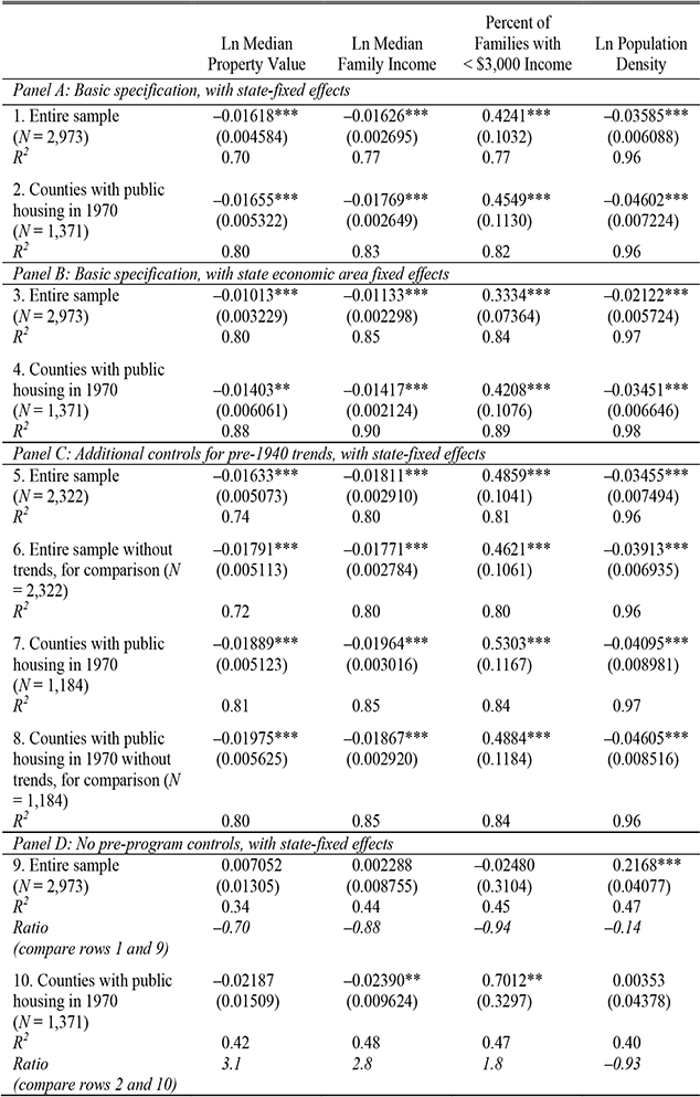
Estimation results of equation 1 are reported in Table 1, panel A, where each coefficient is the estimated  \beta macr from a separate regression. Controlling for Xcounty , 1940 and state-fixed effects, counties with relatively high levels of public housing in 1970 also had relatively high concentrations of low-income families, as well as lower median family income, median property values, and population density. A one percentage point increase in public housing concentration is associated with a 0.42 percentage point increase in families with less than $3,000 income (compared to an average level of 16.7 percent) and is statistically significant at the 1 percent level.Footnote 20 The same increase in public housing intensity is also correlated with a 1.6 percent decrease in median property values, a 1.6 percent decrease in median family income, and a 3.6 percent decrease in population density (all at a 1 percent level of statistical significance). Results are similar when the sample is restricted to counties with a positive amount of public housing in 1970 (also reported in Table 1, panel A) and are robust to the exclusion of counties with the highest intensities (above the 95th percentile) of public housing.Footnote 21
Results with State Economic Area Fixed Effects
The potential for unobservable shocks and trends within states threatens the credibility of the identification strategy in equation 1. One can imagine counties that are observationally similar circa 1940, but distant from one another within the state, and therefore subject to different shocks. With this in mind, I test the sensitivity of the base results by running the regressions again, replacing the state-fixed effects with a much larger set of State Economic Area (SEA) fixed effects. SEAs are comprised of contiguous counties with similar economic characteristics around 1950, as defined by the Census Bureau.Footnote 22 There are 506 SEAs in my sample, and the median SEA contains four counties. Because SEAs are composed of economically similar counties in close proximity, counties within a given SEA should experience similar economic trends or shocks.
Results identified from within-SEA variation in PH are reported in Table 1, panel B. I still find that public housing intensity in 1970 is significantly correlated with relatively low median property values, median family income, and population density, and a relatively high percentage of low-income families in 1970. The magnitudes of the point estimates are somewhat smaller (by approximately one-third relative to Table 1, panel A estimates), but are statistically significant at the 1 percent level and consistent with public housing having economically significant negative effects on local outcomes. When I limit the sample to counties with public housing in 1970, the point estimates using state- and SEA-fixed effects are closer in magnitude, with the SEA-fixed effects results being only 7.5–25 percent smaller than those using state-fixed effects. While some scope for omitted variable bias still exists, the strong empirical links between public housing and local outcomes even within-SEAs (and conditional on pre-program characteristics) are striking.Footnote 23
Results with Pre-1940 Population Trends
The results presented thus far control for a large set of 1940 pre-program characteristics and geographic fixed effects. However, these variables control for counties' characteristics at a fixed point in time and may not pick up differences in underlying growth. The majority of my 1940 controls are not available for previous years, however I do have information on the total population, black population, and number of dwelling units in each county in 1900, 1910, 1920, and 1930. If counties were building public housing as a response to changes in population (not simply 1940 population levels), then adding controls for changes in these variables would reduce the public housing coefficient. I run the regressions again with state-fixed effects, adding controls for the percent change in total population, black population, and number of dwelling units between 1900–1910, 1910–1920, 1920–1930, and 1930–1940. Adding these controls leaves me with a somewhat reduced sample (2,322 observations compared to 2,973), so I run the base regression without trends again with the limited sample, for comparison. Results are reported in Table 1, panel C. While my sample size is somewhat reduced, the magnitude and statistical significance of my public housing coefficients remain virtually unchanged. For example, in a regression of log median property values on public housing intensity, 1940 controls, pre-1940 population and dwelling unit trends, and state-fixed effects, the public housing coefficient is −0.016, compared to −0.018 for the same sample without controlling for pre-program trends, and −0.016 using the original sample (reported in Table 1, panel A, also without trend controls). Results are similar for the other outcomes as well, and are not sensitive to the exclusion of counties without public housing.Footnote 24
Observables, Unobservables, and Causal Interpretation
The robustness of the results to SEA-fixed effects and to pre-program population trends suggest that public housing may indeed have had negative effects on outcomes in 1970. However, omitted variables might still confound the estimated correlation between public housing and outcomes. For example, a county declining in ways that are unobservable to an econometrician might experience a fall in income and an increase in demand for (and supply of) public housing. In this scenario, the cross-place variation of PH is not driven by quasi-random, idiosyncratic local factors, but rather by unobserved negative trends.
To assess how strong such unobserved factors would have to be for the true causal link between PH and Y to be zero, I use a procedure formulated by Joseph G. Altonji, Todd E. Elder, and Christopher R. Taber (2005). John Bellows and Edward Miguel (2009) adapt this technique for a linear framework, and I follow their structure below.Footnote 25
PUBLIC HOUSING AND COUNTY-LEVEL ECONOMIC OUTCOMES IN 1970
* = Significant at the 10 percent level.
** = Significant at the 5 percent level.
*** = Significant at the 1 percent level.
Notes:
Each coefficient is from a separate OLS regression of an economic outcome on public housing intensity and control variables, where public housing intensity is defined as (public housing units in 1970 / total occupied units in 1970 * 100). Pre-program controls included in panels A–C are: 1940 percent owner occupied housing, median persons per room in rental units, percent of units in good condition, percent of units with electricity, percent of units with water, log median value, percent urban, percent high school graduates, percent college graduates, log population density, percent black and percent black squared, percent of the labor force employed in manufacturing, and percent of the labor force employed in agriculture; the value of 1940–1945 World War II contracts and war facilities projects per capita; the percentage of votes for Roosevelt in 1940; and percentages of Baptists and Catholics in 1950. Panel C includes additional controls for the percent change in total population, black population, and number of dwelling units between 1900–1910, 1910–1920, 1920–1930, and 1930–1940. State fixed effects are included in panels A, C, and D. State economic area fixed effects are included in panel B. In all panels, standard errors are reported in parentheses and are clustered by state. Ratios reported in panel D are calculated as βC / (βNC − βC), where βC is the estimated coefficient of the percent of public housing units in 1970 in a regression with controls (panel A) and βNC is the estimated coefficient of the percent of public housing units in 1970 in a regression with no controls (panel D).
Sources:
County population and housing data are from Haines (Reference Haines2004). Data on 1940 presidential election results are from Leip (Reference Leip2009). Public housing data are from the Consolidated Development Directory (HUD 1973).
The Altonji, Elder, and Taber approach centers on a comparison of coefficient estimates from regressions with and without controls for observables. In theory, if the variable of interest were essentially randomly distributed (i.e., there is no selection based on observable or unobservable characteristics), then the coefficient estimated with and without control variables for observables would be the same. In practice, therefore, one might be less concerned about unobservables if adding extensive controls for observables does not diminish the coefficient on the variable of interest. On the other hand, if the coefficient of interest is substantially diminished in magnitude when controls for observable characteristics are added, then one might be particularly concerned that the coefficient estimate would move even closer to zero if one could actually control for additional, unobservable characteristics.
To be more precise, assume that an outcome variable is a function of public housing intensity and an index of community characteristics that may be correlated with public housing. Also assume that the index of community characteristics is a linear function of observable characteristics (X) and unobservable characteristics. The probability limit of an estimated \beta macr is the sum of the true value of β, denoted β0, and the omitted variable bias. In a regression without controls, (where \beta macrNC stands for “no controls”) is equal to β 0 plus the total omitted variable bias (from both observable and unobservable characteristics). Similarly, in a regression with controls for observable characteristics X, the probability limit of \beta macr is equal to β 0 plus the portion of the total omitted variable bias that is not controlled for by X. The difference between and \beta macrNC and \beta macrc is therefore equal to the portion of the total omitted variable bias that can be explained by X.
If the true effect of public housing intensity on outcomes is zero (β 0 = 0), then the value of \beta macrNC is simply equal to the total omitted variable bias, and the value of \beta macrC is the portion of the omitted variable bias attributable to unobservables. Therefore, if the true value of β is zero, then the ratio of the bias explained by unobservables and the bias explained by X (later referred to as the “sensitivity ratio”) can be calculated as \beta_nc(\beta_nc - \beta_c) If the addition of controls diminishes the point estimate by less than half, the sensitivity ratio is greater one. Altonji, Elder, and Taber (Reference Altonji, Elder and Taber2005) argue that “…the ratio of selection on unobservables relative to selection on observables is likely to be less than one…(pp. 176–77),” implying that it is unlikely that the inclusion of unobservables would reduce the point estimate by a greater amount than the inclusion of observables. Therefore, if the addition of controls diminishes the point estimate by less than half (i.e., the sensitivity ratio is greater than one), then the true value of β is not likely to be zero. Footnote 26
I use this technique to assess the direction and strength of selection on unobservables that would be necessary for the true effect of public housing to be equal to zero. Of course, this cannot rule out omitted variable bias in the point estimate, but it allows some appraisal of the plausibility that unobservables drive the basic results. I run regressions without controls for X (but with state-fixed effects), and estimate sensitivity ratios, comparing the estimates from regressions with (Table 1, panel A) and without controls. “No controls” regression results and estimated sensitivity ratios are reported in Table 1, panel D. Without controls for X, public housing intensity is positively correlated with 1970 log median property values, log median family income, and log population density and negatively correlated with the percent of families with low income within states. In fact, it is the addition of my extensive set of controls that causes the public housing coefficient to become negative (or positive in the case of the percent of low-income families) and statistically significant. This causes the sensitivity ratios to be negative. Results are similar using SEA-fixed effects, and suggest that, if anything, county-level selection into public housing on observables was apparently positive.Footnote 27 If the addition of unobservable characteristics pushed the point estimate in the same direction, then the point estimates reported in panel A of Table 1 would be underestimates of the true effect.
However, it is possible that there is positive selection into the program based on observables (for example, urban areas are more likely to adopt public housing), but, conditional on these observables, selection on unobservables is negative. In this scenario, the panel A results would be overestimates. Even if this is the case, the sensitivity ratios indicate that the correlation between public housing and the index of unobservable characteristics would need to be 0.70–0.94 times the magnitude of the correlation between public housing and the index of observable characteristics and be of the opposite sign in order for the true effect of public housing on median property values, median income, and the percent of low-income families to be zero. While one cannot rule out the possibility of negative selection on unobservables, the extensive nature of my controls makes it unlikely that the addition of unobservables could completely reverse the public housing estimate.
As a further check, I run these regressions without pre-program controls (but with state-fixed effects) again, limiting my sample to counties with positive amounts of public housing in 1970. If, conditional on observables, there is negative selection on the extensive margin, then excluding counties that did not participate in the program should address this issue. Results are reported in Table 1, panel D. With the limited sample, public housing is positively correlated with the percent of low-income families and negatively correlated with median property values and median income in regressions with no controls. The addition of 1940 controls diminishes the public housing point estimates slightly, but the sensitivity ratios are large (3.1, 2.9, and 1.9 for log median property values, log median income, and the percent of low-income families, respectively). This suggests that, after controlling for selection on the extensive margin, the correlation between public housing and the index of unobservable characteristics would have to be two to three times the magnitude of the correlation between public housing and the index of observables in order for omitted variable bias to explain the entire effect.Footnote 28
URBAN AND NONURBAN COUNTIES
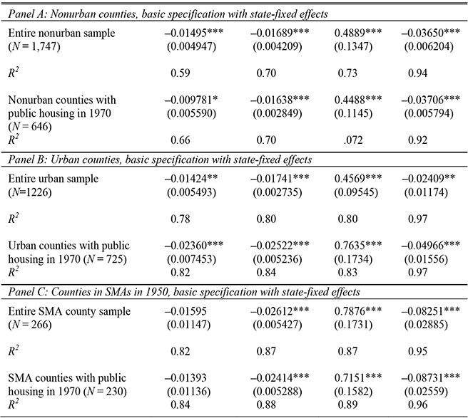
Given that most of the criticism of public housing predominantly focuses on large cities, it is possible that the experiences of urban areas were different from those of nonurban areas. To assess these differences, I estimate equation 1 again, separating my sample by urban status. I define “urban” counties as counties with more than 25 percent urban population in 1940. Because my urban definition is broad, I also run the regressions with a more restricted sample of counties in a Standard Metropolitan Area (SMA) in 1950. Results are reported in Table 2, and suggest that public housing had negative effects in urban and nonurban counties. The point estimates for the log median property value and log median income regressions are similar for urban and nonurban counties (–0.014 and −0.017 for urban counties, compared to −0.015 and −0.017 for nonurban counties, respectively) when using the whole sample. However, the public housing effects appear to be larger for urban areas when the sample is limited to counties with public housing in 1970. For example, using the limited sample, the point estimates for the log median property value and log median income regressions are −0.024 and −0.025 for urban counties, compared to −0.0098 and −0.016 for nonurban counties. The effects of public housing are larger for counties located in SMAs in 1950 for all outcomes. For example, the point estimate of public housing in the log population density regression is −0.083 for counties in SMAs, compared to −0.024 for counties with more than 25 percent urban population. For log median income, the public housing estimate is −0.026 for counties in SMAs, compared to −0.017 for urban counties.
THE EFFECTS OF PUBLIC HOUSING OVER TIME
Effects of Public Housing in 1950 and 1960
Public housing appears to have had negative effects on adopting communities in 1970, but it is unclear whether these effects existed in earlier periods. It is possible that public housing, when relatively new and under the original rules of tenant selection, had no negative effects(or potentially positive effects) on local communities. However, given the disappointment many supporters of the program felt with public housing as early as the late 1950s, these negative effects may have been present earlier. To assess whether the negative relationship between public housing and community outcomes was in place prior to 1970, I estimate equation 1 for similar outcome measures in 1960 and 1950, using public housing intensity measures that are specific to those years. The set of 1940 control variables are the same as for the earlier analysis and state-fixed effects are included.
PUBLIC HOUSING AND COUNTY-LEVEL ECONOMIC OUTCOMES IN 1970, BY URBAN STATUS
* = Significant at the 10 percent level.
** = Significant at the 5 percent level.
*** = Significant at the 1 percent level.
Notes:
Each coefficient is from a separate OLS regression of an economic outcome on public housing intensity and control variables, where public housing intensity is defined as (public housing units in 1970 / total occupied units in 1970 * 100). See Table 1 or the text for a list of independent variables. State fixed effects are included in every regression. “Urban” is defined as having more than 25 percent urban population in 1940. Standard errors are reported in parentheses and are clustered by state.
Sources:
County population and housing data are from Haines (Reference Haines2004). Data on 1940 presidential election results are from Leip (Reference Leip2009). Public housing data are from the Consolidated Development Directory (HUD 1973).
PUBLIC HOUSING AND COUNTY-LEVEL ECONOMIC OUTCOMES IN 1950 AND 1960
* = Significant at the 10 percent level.
** = Significant at the 5 percent level.
*** = Significant at the 1 percent level.
Notes:
Each coefficient is from a separate OLS regression of an economic outcome on public housing intensity and control variables, where public housing intensity is defined as (public housing units in 1970(1960, 1950) / total occupied units in 1970(1960, 1950) * 100). See Table 1 or the text for a list of independent variables. State-fixed effects are included in every regression. Standard errors are reported in parentheses and are clustered by state.
Sources:
County population and housing data are from Haines (Reference Haines2004). Data on 1940 presidential election results are from Leip (Reference Leip2009). Public housing data are from the Consolidated Development Directory (HUD 1973).
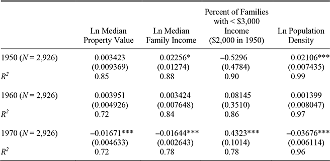
Results are reported in Table 3, and suggest that public housing did not have negative effects on adopting communities before 1970. Public housing was not statistically significantly correlated with log median property values, log median income, the percent of families with less than $3,000 income, or log population density in 1960. Public housing was also not statistically significantly correlated with log median property values, the percent of families with low income, or log median income in 1950. The coefficient on public housing is statistically significant in the log population density regression for 1950, however the coefficient is positive.Footnote 29
Several hypotheses might account for this pattern of results. One possibility is that there were changes in the types of counties adopting or expanding public housing over time. Counties with negative unobservable characteristics could have rapidly adopted or expanded public housing in the 1960s, causing public housing to be correlated with poor community outcomes. Of course, the variety of robustness checks presented above (using SEA-fixed effects, controlling for pre-program trends, and assessing the necessary relative size of the omitted variable bias) suggest that negative selection does not explain the negative public housing effects in 1970.Footnote 30
Another possibility is that long-run changes in the characteristics of public housing are driving the results. For example, the type (high rise, low rise, scattered site) or quality of public housing built could have varied by decade of construction. If higher density or lower quality public housing was built in the 1960s, then public housing built during this decade may have led to larger negative effects than older, higher-quality, less densely populated public housing. On the other hand, the negative effects may have nothing to do with public housing built in the 1960s specifically, but could be due to the long-run deterioration of projects like Salisbury (Reference Salisbury1958) observed in New York City. Even though the process of decay started decades earlier in some places, it may have taken until the 1960s for local economies to adjust and for these effects to be detectible at the county level. Or, the effects of public housing may not be related to the physical characteristics of the units (such as age or style), but to issues related to poor management by local housing authorities and changing tenant characteristics (Weicher Reference Weicher1980).
Effects of Public Housing in 1970, by Date of Construction
It is difficult to empirically distinguish between all these possibilities. However, I can explore whether a rapid expansion of public housing during the 1960s can explain the base results. If public housing built in the 1960s is largely driving my results, then the proportion of housing units composed of public housing built in the decades before 1960 should not be negatively correlated with 1970 outcomes. This would be consistent with either negative decade-specific selection into the program, or “worse” public housing built in the 1960s, as the quality of construction is rumored to have decreased. On the other hand, it is possible that old units have large effects on outcomes because of long-run deterioration of buildings or because units have had a longer time to create negative spillovers large enough to be measured in county-level aggregates.
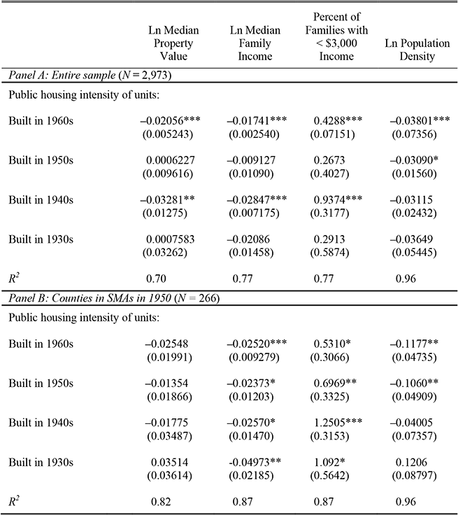
To assess whether public housing built in the 1960s is driving my 1970 results, I estimate equation 1 again, allowing for separate effects of public housing built in the 1930s, 1940s, 1950s, and 1960s. Public housing built in each decade is measured as the percent of total occupied units in 1970 composed of public housing units built in that particular decade. Results are reported in Table 4, panel A. Public housing built in the 1940s generally has the largest effects on outcomes. For example, a one percentage point increase in the intensity of public housing built in the 1940s is correlated with a 3.3 percent decrease in median property values (compared to a 1.6 percent decrease in Table 1, panel A). This is consistent with either 1940s public housing having a longer amount of time to affect community outcomes, or with 1940s public housing being of lower quality than other public housing units in 1970, due to prolonged lack of maintenance.
Public housing built in the 1960s has the second largest effects. A one percentage point increase in the intensity of public housing built in the 1960s is correlated with a 2.1 percent decrease in median property values. Similar increases in the intensity of public housing built in the 1940s and 1960s are correlated with a 2.8 and a 1.7 percent decrease in median family income, respectively. The point estimates for public housing built in the 1950s are consistent with it having adverse effects on 1970 median income, population density, and the percent of low-income families, although the estimates for median income and the percent of low-income families are not statistically significant. However, the estimated coefficient on the effects of 1950s public housing construction on median property values is very low. The results are also weaker for public housing built in the 1930s. This could be due to selection into the program, as only 88 of the 2,973 counties completed public housing projects before 1940.
It is unclear why the results are weaker for public housing built in the 1950s, particularly given the criticism that many of the projects in large cities received during this decade. Because much of the criticism focused on high rises, which were concentrated in large cities, it is possible that these negative effects exist in metropolitan areas but are being suppressed by the nonmetropolitan counties in my sample. To assess whether this pattern is present in metropolitan areas, I estimate these regressions again, limiting my sample to counties within Standard Metropolitan Areas (SMAs) in 1950. Results are reported in Table 4, panel B. For this sample, public housing built in every decade appears to have an adverse and statistically significant effect on median income and the percent of low-income families. The results are also consistent with public housing built in the 1940s, 1950s, and 1960s having similar negative effects on median property value, however these coefficients are not statistically significant. The point estimate on public housing built in the 1930s is positive, although it also is not statistically significant.
PUBLIC HOUSING AND HUMAN CAPITAL
Public Housing and Local Human Capital, 1950–1970
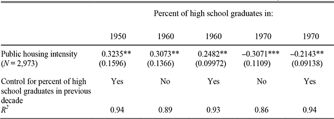
It is difficult to decipher the channels through which public housing negatively affected outcomes in 1970. However, one possibility is that public housing worsened economic outcomes by negatively affecting the educational composition of the population. To better understand the relationship between public housing and human capital, I first assess whether public housing is correlated with the education level of county residents between 1950 and 1970. I regress the percent of the population composed of high school graduates in each decade on public housing intensity in that decade, 1940 pre-program characteristics, and state-fixed effects (equation 1). I also run the 1960 and 1970 regressions again, adding a control for the percent of high school graduates in the previous decade.Footnote 31 Results are reported in Table 5.
I find that public housing is positively correlated with the percent of high school graduates in 1950 and 1960. A one percentage point increase in public housing intensity is correlated with a 0.25–0.32 percentage point increase in the percent of high school graduates in each of these two decades. By 1970, however, the relationship between public housing and the percent of high school graduates reversed. By this point, a one percentage point increase in public housing is correlated with a 0.21–0.31 percentage point decline in the percent of high school graduates.
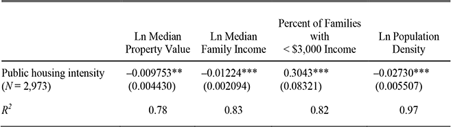
Next, I assess whether public housing's negative correlation with economic outcomes in 1970 is accounted for by the negative correlation between public housing and the local population's educational attainment. I estimate equation 1 again for log median property values, log median income, the percent of low income families, and log population density, this time adding a control for the percent of high school graduates in 1970. The percent of high school graduates in 1970 is likely endogenous to public housing, and so the coefficient on PH should not be interpreted as a causal effect of public housing intensity when the 1970 control is included. However, observing how the public housing coefficient changes with the addition the endogenous control will shed light on whether the change in the educational composition of the population is driving the base results. Results are reported in Table 6.
PUBLIC HOUSING AND COUNTY-LEVEL ECONOMIC OUTCOMES IN 1970, BY DECADE OF CONSTRUCTION
Notes:
* = Significant at the 10 percent level.
** = Significant at the 5 percent level.
*** = Significant at the 1 percent level.
Notes:
Public housing intensity built in each decade is defined as (# public housing units built in the 1930s (or 40s, 50s, 60s) / total occupied units in 1970 * 100). See Table 1 or the text for a list of independent variables. State-fixed effects are included in every regression. Standard errors are reported in parentheses and are clustered by state.
Sources:
County population and housing data are from Haines (Reference Haines2004). Data on 1940 presidential election results are from Leip (Reference Leip2009). Public housing data are from the Consolidated Development Directory (HUD 1973).
In these regressions, controlling for 1970 educational composition reduces the coefficient on public housing by between 24 and 40 percent. For log median property values, controlling for the educational composition of the 1970 population causes the coefficient on public housing to fall from −0.016 (Table 1, panel A) to −0.0098 (statistically significant at the 5 percent level), while the coefficient in the log median family income regression falls from −0.016 to −0.012 (statistically significant at the one percent level). The coefficient falls from 0.42 to 0.30 for the percent of families with low income, and falls from −0.036 to −0.027 for log population density (both statistically significant at the 1 percent level). This pattern suggests that part, but not all, of the estimated effects of public housing on the outcome variables of interest might work through effects on the educational attainment of the local population.
Public Housing and Selective Migration
There are several ways in which public housing may have negatively affected educational attainment. As discussed earlier, it is possible that public housing lowered human capital by creating perverse education and labor market incentives for local residents. Or, public housing may have influenced human capital through selective migration, either by encouraging low education residents to move into the locality, or by encouraging high education residents to move out. Depending on the mechanism, public housing may have decreased the percent of high school graduates either by increasing the population of high school dropouts, or by decreasing the population of high school graduates. If public housing created negative educational incentives for locals and/or encouraged the in-migration of low-human capital residents, then public housing would be correlated with an increase in the population of high school dropouts. On the other hand, if public housing encouraged the outmigration of high school graduates, it is possible for public housing to be negatively correlated with the percent of high school graduates, even if it is not correlated with an increase in the number of high school dropouts.
PUBLIC HOUSING AND COUNTY-LEVEL EDUCATIONAL ATTAINMENT, 1950–1970
* = Significant at the 10 percent level.
** = Significant at the 5 percent level.
*** = Significant at the 1 percent level.
Notes:
Each coefficient is from a separate OLS regression of an economic outcome on public housing intensity and control variables, where public housing intensity is defined as (public housing units in 1970 / total occupied units in 1970 * 100). See Table 1 or the text for a list of independent variables. State-fixed effects are included in every regression. Standard errors are reported in parentheses and are clustered by state.
Sources:
County population and housing data are from Haines (Reference Haines2004). Data on 1940 presidential election results are from Leip (Reference Leip2009). Public housing data are from the Consolidated Development Directory (HUD 1973).
PUBLIC HOUSING AND COUNTY-LEVEL ECONOMIC OUTCOMES IN 1970, CONTROLLING FOR THE PERCENT OF HIGH SCHOOL GRADUATES IN 1970
Notes:
* = Significant at the 10 percent level.
** = Significant at the 5 percent level.
*** = Significant at the 1 percent level.
Notes:
Each coefficient is from a separate OLS regression of an economic outcome on public housing intensity and control variables, where public housing intensity is defined as (public housing units in 1970 / total occupied units in 1970 * 100). See Table 1 or the text for a list of independent variables. State-fixed effects are included in every regression. Standard errors are reported in parentheses and are clustered by state.
Sources:
County population and housing data are from Haines (Reference Haines2004). Data on 1940 presidential election results are from Leip (Reference Leip2009). Public housing data are from the Consolidated Development Directory (HUD 1973).
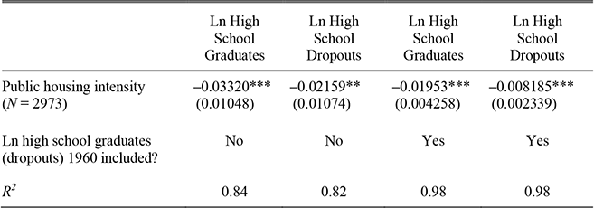
To better understand this relationship between public housing and human capital, I assess whether public housing is correlated with a larger population of high school dropouts or a smaller population of high school graduates in 1970. I do this by running equation 1 again, using the log number of high school graduates and dropouts as my variables of interest. Results are reported in Table 7. The point estimates on public housing intensity in the regressions of the log number of high school graduates and the log number of high school dropouts in 1970 are −0.033 and −0.022, respectively (statistically significant at the 1 and 5 percent levels). This suggests that a one percentage point increase in public housing intensity is correlated with a 3.3 percent decline in the population of high school graduates, but only a 2.2 percent decline in the number of high school dropouts. When I run the regressions again, adding controls for the log number of high school graduates (dropouts) in 1960, the point estimates fall to −0.020 and −0.0082. However, both remain statistically significant and the coefficient for the number of high school graduates is more than twice the magnitude of the coefficient for the number of high school dropouts. This is consistent with public housing encouraging the out-migration of both high- and low-education residents, however the low-education residents appear to leave more slowly than those with a high school degree.
Public Housing and Rates of In-Migration
The results above indicate that places with high intensities of public housing experienced a net loss in the population of high school graduates and dropouts. However, it is still possible that public housing encouraged the selective in-migration of high school dropouts who wanted to take advantage of public housing, while simultaneously encouraging a larger outflow of others without a high school degree. To further assess the relationship between public housing and selective migration, I incorporate data on migration rates for 1960 and 1970. Data from the 1960 and 1970 Population Censuses (U.S. Bureau of the Census Reference Grigsby1963, 1973) and the 1970 micro-Census (Ruggles et al. Reference Ruggles, Alexander, Genadek, Goeken, Schroeder and Sobek2010) report whether individuals lived in the same county five years previously. I use these data to assess whether areas with high densities of public housing had higher or lower percentages of their populations composed of recent in-migrants in 1960 and 1970, and to assess whether these migration trends differ by educational attainment in 1970.
PUBLIC HOUSING AND THE POPULATION OF HIGH SCHOOL GRADUATES AND DROPOUTS IN 1970
Notes:
* = Significant at the 10 percent level.
** = Significant at the 5 percent level.
*** = Significant at the 1 percent level.
Notes:
Each coefficient is from a separate OLS regression of an economic outcome on public housing intensity and control variables, where public housing intensity is defined as (public housing units in 1970 / total occupied units in 1970 * 100). See Table 1 or the text for a list of independent variables. State-fixed effects are included in every regression. Standard errors are reported in parentheses and are clustered by state.
Sources:
County population and housing data are from Haines (Reference Haines2004). Data on 1940 presidential election results are from Leip (Reference Leip2009). Public housing data are from the Consolidated Development Directory (HUD 1973).
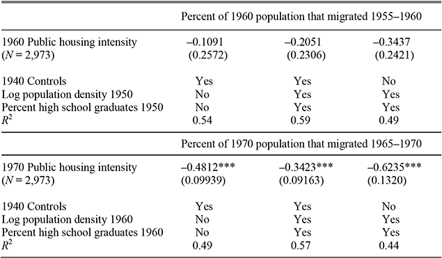
I begin by assessing whether areas with high densities of public housing in 1960 or 1970 had higher or lower percentages of recent in-migrants in those years.Footnote 32 I regress the percent of recent in-migrants (the percent of the 1970 (1960) population who migrated into a county between 1965–1970 (1955–1960)) on 1940 pre-program characteristics and state-fixed effects (equation 1). I then run the regressions again, adding controls for log population density and the percent of high school graduates in the previous decade. Finally, I run the regressions a third time, controlling only for log population density and the percent of high school graduates in the previous decade, for comparison with future results. Results are reported in Table 8.
In 1960 public housing intensity is negatively correlated with the percent of recent migrants in all specifications, although none of the point estimates are statistically significant. In 1970 this negative relationship increases in magnitude and becomes statistically significant at the 1 percent level in all three specifications. Depending on the specification, a one percentage point increase in public housing intensity is correlated with a 0.34–0.62 percentage point decline in the percent of the population composed of recent migrants. This is not consistent with an in-migration story.
PUBLIC HOUSING AND THE PERCENT OF RECENT MIGRANTS IN 1960 AND 1970, BY COUNTY
Notes:
* = Significant at the 10 percent level.
** = Significant at the 5 percent level.
*** = Significant at the 1 percent level.
Notes:
Each coefficient is from a separate OLS regression of an economic outcome on public housing intensity and control variables, where public housing intensity is defined as (public housing units in 1970 / total occupied units in 1970 * 100). See Table 1 or the text for a list of independent variables. State fixed effects are included in every regression. Standard errors are reported in parentheses and are clustered by state.
Sources:
County population and housing data are from Haines (Reference Haines2004). Data on 1940 presidential election results are from Leip (Reference Leip2009). Public housing data are from the Consolidated Development Directory (HUD 1973). Migration rates come from the Population Census of 1960 and 1970 (U.S. Bureau of the Census, Reference Grigsby1963 and 1973).
Public Housing and Rates of In-Migration, by Educational Attainment
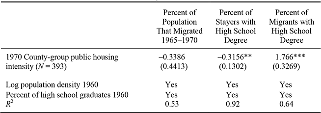
Finally, I assess whether public housing had different migration “effects” on high and low human capital residents by incorporating data from the 1970 micro-Census (Ruggles et al. Reference Ruggles, Alexander, Genadek, Goeken, Schroeder and Sobek2010). The 1970 individual-level census data does not report an individual's county of residence, but it does report the “county-group” in which an individual resides.Footnote 33 The census also reports whether an individual lived in a different county in 1965. Using these data, I divide each county-group's 1970 adult population (age 20+) into four groups based on educational attainment (high school graduate or dropout) and 1965 residence (same county (stayer) or different county (migrant)).
For comparison with the county sample, I begin by regressing the percent of a county-group's 1970 population (both high school graduates and dropouts) that lived in a different county in 1965 on 1970 county-group public housing intensity, 1960 county-group log population density and percent of high school graduates, and census division fixed effects.Footnote 34

Next, I estimate equation 2 again, using the percent of the “stayer” population (those who lived in the same county in 1965 and 1970) composed of high school graduates and the percent of the migrant population composed of high school graduates in 1970 as my variables of interest. If public housing is negatively correlated with the educational attainment of stayers, then this would be consistent with public housing encouraging the out-migration of high human capital residents, or discouraging the educational attainment of local residents. If public housing is negatively correlated with the educational attainment of recent migrants, then this would be consistent with public housing encouraging the in-migration of low-human capital residents. Results are reported in Table 9.
I find that public housing intensity is negatively correlated with the percent of the 1970 population composed of recent migrants, which is consistent with the earlier county-level results. The estimated coefficient on public housing intensity is −0.34, although it is not statistically significant. I also find that public housing intensity is negatively correlated with the percent of stayers who are high school graduates in 1970. A one percentage point increase in public housing intensity is correlated with a 0.32 percentage point decrease in the percent of stayers who are high school graduates (statistically significant at the 1 percent level). However, public housing is not correlated with a less educated stock of recent migrants. In fact, public housing is correlated with a 1.77 percentage point increase in the percent of recent migrants with a high school degree. This is consistent with public housing encouraging the out-migration of high school graduates or discouraging educational attainment among locals, but not consistent with public housing encouraging the in-migration of low human capital residents.
PUBLIC HOUSING AND THE PERCENT OF RECENT MIGRANTS BY EDUCATIONAL ATTAINMENT 1970, BY COUNTY-GROUP
Notes:
* = Significant at the 10 percent level.
** = Significant at the 5 percent level.
*** = Significant at the 1 percent level.
Notes:
Each coefficient is from a separate OLS regression of an economic outcome on public housing intensity and control variables, where public housing intensity is defined as (public housing units in 1970 / total occupied units in 1970 * 100). Census division fixed effects are included in each regression. Standard errors are reported in parentheses and are clustered by census division.
Sources:
County-group 1970 public housing intensity, 1960 log population density, and 1960 percent of high school graduates are calculated by aggregating county-level data (HUD 1973; Haines Reference Haines2004). The percent of the population who migrated between 1965 and 1970, the percent of stayers who are high school graduates, and the percent of migrants who are high school graduates are aggregated from individual-level 1970 Census data (Ruggles et al. Reference Ruggles, Alexander, Genadek, Goeken, Schroeder and Sobek2010).
CONCLUSIONS
Federally funded low-income public housing originated as a response to decades of concern about the quality of housing for the nation's poor. The program was controversial from its inception in the 1930s, and in the mid-1970s, construction of new public housing was temporarily halted as policy shifted toward a voucher system. It was widely believed that public housing projects had deteriorated into the slums that they were meant to replace. Nonetheless, most of the projects built by the 1970s are still in operation, and a better understanding of their effects on adopting communities would be valuable.
Using new data from the Consolidated Development Directory, I am able to estimate the effects of public housing on population and housing market outcomes for localities in the period up to 1970, before the major policy shift away from public housing construction. I find that public housing is associated with adverse 1970 county-level outcomes such as low median income, low median property values, low population density, and a high percentage of low-income families. Further tests suggest that these relationships are causal. These effects are largest in metropolitan areas, however public housing appears to have negative effects on nonurban counties as well.
It is important to note that public housing had no measurable negative effect on outcomes in 1950 or 1960. This suggests that public housing was not always “bad.” It is unclear why this correlation between public housing and economic effects suddenly appears in the 1960s. One possibility is that it is due to the changing nature of public housing, with regard to both its physical and tenant characteristics. The long-run deterioration of buildings and the increased presence of single-parent and chronically poor households within public housing may have increased the disamenities associated with public housing projects.
It is also difficult to decipher the exact channels through which public housing affected communities. However, I find that changes in the educational composition of the population account for part, but not all, of the public housing effect on other economic outcomes. Moreover, this link does not appear to work through the attraction of low human-capital migrants. It appears that public housing was correlated with lower educational attainment of nonmigrants, which is consistent with either the outmigration of high human-capital residents, or decreased educational achievement among local residents. Further research will be necessary to uncover the nature of the strongly negative turn in public housing's association with local outcomes during the 1960s.