1 Introduction
The electromagnetic force that results from the interaction of an electric current with its own magnetic field is usually rotational and, thus, induces a flow when the conducting medium is fluid (Bojarevičs et al. Reference Bojarevičs, Freibergs, Shcherbinin and Shilova1989). However, some rotationally or translationally invariant current distributions can produce a purely potential electromagnetic force which can be balanced by the pressure gradient alone. Such quiescent equilibrium states are not always stable and can collapse when subject to an arbitrary small disturbance. The prominent example is the electromagnetic pinch, which can disrupt or kink conductors carrying strong electric currents (Haines et al. Reference Haines, Lebedev, Chittenden, Beg, Bland and Dangor2000). It usually affects conducting media with deformable boundaries and has a growth rate determined by the balance of inertia and the characteristic magnetic pressure. This results in the instability that develops with the Alfvén wave speed regardless of the electrical conductivity of the fluid (Tayler Reference Tayler1960). Electromagnetic pinch-type instability can develop also in the incompressible liquids bounded by solid walls (Michael Reference Michael1954). In a perfectly conducting liquid, this internal pinch instability also develops on the Alfvén time scale (Velikhov Reference Velikhov1959). The previous two studies were extended by Tayler (Reference Tayler1961) to general non-axisymmetric instability modes in a perfectly conducting fluid bounded by solid cylindrical walls. Later it was suggested by Vandakurov (Reference Vandakurov1972) and Tayler (Reference Tayler1973) that a similar instability can affect the interiors of stars containing toroidal magnetic fields. The strong stratification in stellar interiors makes this instability nearly horizontal and, thus, significantly different from the pinch instabilities with deformable boundaries (Tayler Reference Tayler1957). In order to stress this difference, Spruit (Reference Spruit1999) termed the astrophysical variety of pinch instability the Tayler instability. This term was later used by Rüdiger et al. (Reference Rüdiger, Hollerbach, Schultz and Elstner2007) in a much broader sense to refer to current-driven instabilities in homogeneous fluids including liquid metals. The latter type of instability, which differs from the Tayler instability not only by the absence of radial stratification but also by its resistive nature, which will be discussed in this paper, was presumably observed in the liquid-metal experiment by Seilmayer et al. (Reference Seilmayer, Stefani, Gundrum, Weier, Gerbeth, Gellert and Rüdiger2012). The notion of Tayler instability is further broadened in the recent study by Herreman et al. (Reference Herreman, Nore, Cappanera and Guermond2015) who refer by it to all pinch-type instabilities studied by Tayler including also the classical case with deformable boundaries (Tayler Reference Tayler1957, Reference Tayler1960).
It is important to note that surface deformation provides an additional pinch instability mechanism. Although surface deformation always involves fluid flow, it is not required for the internal pinch-type instability, which can be driven by the fluid flow alone. In ideally conducting fluid, where the magnetic field is frozen in, flow causes the same-order disturbance of the magnetic field as that associated with the surface deformation, i.e. proportional to the displacement (Tayler Reference Tayler1957). In a poorly conducting liquid, the perturbation of the magnetic field caused by the fluid flow is proportional not to the displacement but to the product of velocity and conductivity. This perturbation is much weaker than that associated with surface deformation (Tayler Reference Tayler1960).
Another peculiarity of internal current-driven instability is its reliance on the curvature of the magnetic field. For example, in the liquid-metal annulus carrying an axial current and bounded by solid walls, instability vanishes when the radius of the gap tends to infinity and, thus, the circular magnetic flux lines straighten out (Priede Reference Priede2015). This is consistent with the absence of purely magnetic instability in the planar perfectly conducting liquid layer permeated by a straight co-planar magnetic field whatever its distribution over the thickness of the layer (Ogilvie & Pringle Reference Ogilvie and Pringle1996). In contrast to cylindrical geometries, where the curvature of the magnetic field is inherent and pinch-type instabilities usually occur, in planar geometries, such instabilities are likely to be induced by the edges and corners, around which the magnetic field bends. Moreover, rectangular configurations may be relevant to the recently developed liquid-metal batteries (Wang et al. Reference Wang, Jiang, Chung, Ouchi, Burke, Boysen, Bradwell, Kim, Muecke and Sadoway2014), for which the electrode mixing (Kelley & Sadoway Reference Kelley and Sadoway2014) due to potential current-driven instabilities is one of the major concerns (Stefani et al. Reference Stefani, Weier, Gundrum and Gerbeth2011; Weber et al. Reference Weber, Galindo, Stefani, Weier and Wondrak2013; Herreman et al. Reference Herreman, Nore, Cappanera and Guermond2015; Weber et al. Reference Weber, Galindo, Priede, Stefani and Weier2015).
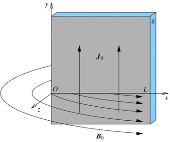
Sketch of the problem.

In this paper we consider an elementary model of pinch-type instability consisting of a semi-infinite planar layer of inviscid conducting liquid that is bounded by solid walls and carries a uniform electric current. This is the simplest possible model of the internal pinch instability in planar geometry. It allows us to elucidate the basic characteristics of the instability, which may otherwise be obscured by technical details of more realistic numerical models and laboratory experiments. In particular, we show that the internal pinch instability is an edge effect caused by the curvature of the magnetic field, and its growth rate is determined by the linear current density and independent of the system size. This suggests that the instability can be prevented either by reducing the field curvature at the edges or by limiting the layer thickness but not its lateral size when the areal current density is fixed. We also point out that the instability is significantly different in well conducting and highly resistive fluids like liquid metals. In the latter, the instability development time depends on the electrical conductivity rather than being determined by the Alfvén wave speed as for the Tayler instability. This somewhat limits the astrophysical significance of liquid-metal laboratory experiments. On the other hand, it implies that this type of instability, if any, in the liquid-metal batteries significantly differs from the Tayler instability in astrophysics.
The paper is organized as follows. Mathematical model is introduced in § 2 and the linear stability problem is formulated in § 3. Numerical method and the main results are presented in §§ 4 and 5. The paper is concluded with a summary and brief discussion of the results in § 6.
2 Formulation of the problem
Consider a channel of width
 $L$
and depth
 $\unicode[STIX]{x1D6FF}$
between two solid vertical parallel walls filled with an inviscid liquid of density
 $\unicode[STIX]{x1D70C}$
and electrical conductivity
 $\unicode[STIX]{x1D70E}$
. The liquid carries electric current of a uniform density
 $\boldsymbol{j}_{0}$
directed upwards along the rigid edge of the channel, which coincides with the
 $y$
-axis of the Cartesian system of coordinates shown in figure 1. The layer is assumed to be thin with
 $\unicode[STIX]{x1D6FF}\ll L$
and, thus, treated as a planar undeformable sheet with the areal density
 $\bar{\unicode[STIX]{x1D70C}}=\unicode[STIX]{x1D70C}\unicode[STIX]{x1D6FF}$
and the respective electrical conductivity
 $\bar{\unicode[STIX]{x1D70E}}=\unicode[STIX]{x1D70E}\unicode[STIX]{x1D6FF}$
. The electric current with the linear density
 $\boldsymbol{J}_{0}=\boldsymbol{e}_{y}j_{0}\unicode[STIX]{x1D6FF}$
that flows along the sheet generates a magnetic field whose normal
 $(z)$
component through the sheet can be found using the Biot–Savart law as
 $$\begin{eqnarray}B_{0}(x)=\frac{\unicode[STIX]{x1D707}_{0}J_{0}}{2\unicode[STIX]{x03C0}}\int _{0}^{L}\frac{\text{d}\unicode[STIX]{x1D709}}{\unicode[STIX]{x1D709}-x}=\frac{\unicode[STIX]{x1D707}_{0}J_{0}}{2\unicode[STIX]{x03C0}}\ln \left(\frac{L}{x}-1\right)\approx \frac{\unicode[STIX]{x1D707}_{0}J_{0}}{2\unicode[STIX]{x03C0}}\ln \frac{L}{x},\end{eqnarray}$$
where the last approximate expression holds in the vicinity of edge for
 $x\ll L$
, which will be the main focus of this study. On the other hand, the sheet approximation implies
 $x\gg \unicode[STIX]{x1D6FF}$
. Note that expression (2.1) represents a superposition of the fields of straight wires which may be thought to form the sheet. As only the gradient of the field
 $B_{0}^{\prime }(x)\approx -(\unicode[STIX]{x1D707}_{0}J_{0}/2\unicode[STIX]{x03C0}x)$
is required in the following, the width
 $L$
drops out of the model. It means that the layer is treated as semi-infinite. The interaction of the electric current with its own magnetic field gives rise to the pinch force with the areal density
 $\boldsymbol{F}_{0}=\boldsymbol{J}_{0}\times \boldsymbol{B}_{0}=\boldsymbol{e}_{x}J_{0}B_{0}(x)$
, which is balanced by the
 $x$
-component of the effective pressure gradient
 $$\begin{eqnarray}P_{0}^{\prime }(x)=-J_{0}B_{0}(x).\end{eqnarray}$$
Note that for sheet, the effective pressure
 $P$
is defined as force per unit length.
Disturbance of this quiescent equilibrium state by an arbitrary slow liquid flow, which is confined to the plane of the sheet by the solid bounding walls, is governed by the linearized two-dimensional (2-D) Euler’s equation
 $$\begin{eqnarray}\bar{\unicode[STIX]{x1D70C}}\unicode[STIX]{x2202}_{t}\boldsymbol{v}_{1}=-\unicode[STIX]{x1D735}P_{1}+\boldsymbol{F}_{1},\end{eqnarray}$$
with the velocity distribution
 $\boldsymbol{v}_{1}$
subject to the incompressibility constraint
 $\unicode[STIX]{x1D735}\boldsymbol{\cdot }\boldsymbol{v}_{1}=0$
. The linearized perturbation of the electromagnetic force
 $\boldsymbol{F}_{1}=(\boldsymbol{J}_{1}B_{0}+\boldsymbol{J}_{0}B_{1})\times \boldsymbol{e}_{z}$
produced by the flow results from the interaction of the current perturbation
 $\boldsymbol{J}_{1}$
with the base magnetic field
 $B_{0}$
as well as from the interaction of the base current
 $\boldsymbol{J}_{0}$
with the perturbation of the normal magnetic field
 $B_{1}$
. Note that the quadratic terms in the perturbation amplitudes are neglected as usual in the linear stability analysis because all perturbations are assumed to be infinitesimal. The perturbation of the pressure gradient
 $\unicode[STIX]{x1D735}P_{1}$
is eliminated from (2.3) by applying the curl operator. Then the flow is governed by the
 $z$
-component of the resulting equation
 $$\begin{eqnarray}\bar{\unicode[STIX]{x1D70C}}\unicode[STIX]{x2202}_{t}\unicode[STIX]{x1D714}_{1}=-(\boldsymbol{J}_{1}\boldsymbol{\cdot }\unicode[STIX]{x1D735}B_{0}+\boldsymbol{J}_{0}\boldsymbol{\cdot }\unicode[STIX]{x1D735}B_{1}),\end{eqnarray}$$
where
 $\unicode[STIX]{x1D714}_{1}=\boldsymbol{e}_{z}\boldsymbol{\cdot }\unicode[STIX]{x1D735}\times \boldsymbol{v}_{1}$
is the normal component of vorticity. The associated current perturbation is governed by Ohm’s law for a moving medium
 $$\begin{eqnarray}\boldsymbol{J}_{1}=\bar{\unicode[STIX]{x1D70E}}(\boldsymbol{E}_{1}+\boldsymbol{v}_{1}\times \boldsymbol{e}_{z}B_{0}).\end{eqnarray}$$
A time-dependent perturbation of the magnetic field induces a rotational electric field according to the first Maxwell equation
 $\unicode[STIX]{x1D735}\times \boldsymbol{E}_{1}=-\unicode[STIX]{x2202}_{t}\boldsymbol{B}_{1}$
. Note that in highly resistive media this induction effect is usually negligible, which corresponds to the so-called quasi-stationary or inductionless approximation commonly used in the liquid-metal MHD (Roberts Reference Roberts1967). In order to keep our model general and applicable also to well conducting fluids, we forgo this approximation here.
The charge conservation
 $\unicode[STIX]{x1D735}\boldsymbol{\cdot }\boldsymbol{J}_{1}=0$
is satisfied by introducing the electric streamfunction
 $h_{1}$
, which, as shown below, is directly related to the scalar magnetic potential at the current sheet. It allows us to represent the electric current in the plane of sheet as
 $$\begin{eqnarray}\boldsymbol{J}_{1}=-\boldsymbol{e}_{z}\times \unicode[STIX]{x1D735}h_{1}.\end{eqnarray}$$
Note that a truly 2-D (
 $z$
-independent) current distribution would generate a 2-D magnetic field with
 $z$
-component only which would then coincide with the current streamfunction introduced above. The current sheet considered here, however, produces a 3-D magnetic field whose normal component at the sheet is related with the electric stream function by the induction-type equation which is obtained as follows. Substituting (2.6) into (2.5) and taking the
 $z$
-component of the curl of the resulting equation, we obtain
 $$\begin{eqnarray}\unicode[STIX]{x2202}_{t}B_{1}+\boldsymbol{v}_{1}\boldsymbol{\cdot }\unicode[STIX]{x1D735}B_{0}=\bar{\unicode[STIX]{x1D70E}}^{-1}\unicode[STIX]{x1D6FB}^{2}h_{1}.\end{eqnarray}$$
The magnetic field perturbation in the surrounding space is sought as
 $$\begin{eqnarray}\boldsymbol{B}_{1}=-\unicode[STIX]{x1D707}_{0}\unicode[STIX]{x1D735}\unicode[STIX]{x1D6F9}_{1}\end{eqnarray}$$
using the scalar magnetic potential
 $\unicode[STIX]{x1D6F9}_{1}$
, which is governed by the Laplace equation
 $$\begin{eqnarray}\unicode[STIX]{x1D6FB}^{2}\unicode[STIX]{x1D6F9}_{1}=0.\end{eqnarray}$$
The surface current density is related to the jump of the tangential magnetic field over the current sheet by Ampère’s circuital law:
 $\boldsymbol{J}_{1}=(1/\unicode[STIX]{x1D707}_{0})\boldsymbol{e}_{z}\times [\boldsymbol{B}_{1}]_{S}$
, where
 $\unicode[STIX]{x1D707}_{0}=4\unicode[STIX]{x03C0}\times 10^{-7}~\text{H}~\text{m}^{-1}$
is the vacuum permeability. Combining this current sheet condition with (2.6) and (2.8), we obtain the boundary condition
 $$\begin{eqnarray}\unicode[STIX]{x1D6F9}_{1}|_{z\rightarrow +0}=-\unicode[STIX]{x1D6F9}_{1}|_{z\rightarrow -0}={\textstyle \frac{1}{2}}h_{1},\end{eqnarray}$$
which relates the scalar magnetic potential with the electric stream function. It is important to note that the problem is defined in terms of the linear current density
 $J_{0}$
, which is the relevant electromagnetic parameter in the current sheet approximation.
3 Linear stability analysis
Owing to the
 $y$
-invariance of the base state, perturbations can be sought in the normal mode form
 $$\begin{eqnarray}\{\boldsymbol{v}_{1},p_{1},h_{1}\}(\boldsymbol{x},t)=\{\hat{\boldsymbol{v}},\hat{p},{\hat{h}}\}(x)\text{e}^{\unicode[STIX]{x1D6FE}t+\text{i}ky},\end{eqnarray}$$
where
 $\unicode[STIX]{x1D6FE}$
is a generally complex growth rate and
 $k$
is a real wavenumber. Then (2.4) and (2.7) for the flow and current perturbations take the form
 $$\begin{eqnarray}\displaystyle & \displaystyle \unicode[STIX]{x1D6FE}\boldsymbol{D}_{k}^{2}\hat{v}=-\bar{\unicode[STIX]{x1D70C}}^{-1}J_{0}k^{2}\left(\hat{B}+\frac{\unicode[STIX]{x1D707}_{0}}{2\unicode[STIX]{x03C0}}\frac{{\hat{h}}}{x}\right), & \displaystyle\end{eqnarray}$$
 $$\begin{eqnarray}\displaystyle & \displaystyle \unicode[STIX]{x1D6FE}\hat{B}=\bar{\unicode[STIX]{x1D70E}}^{-1}\boldsymbol{D}_{k}^{2}{\hat{h}}+J_{0}\frac{\unicode[STIX]{x1D707}_{0}}{2\unicode[STIX]{x03C0}}\frac{\hat{v}}{x}, & \displaystyle\end{eqnarray}$$
where
 $\hat{v}$
is the
 $x$
-component of the velocity perturbation, which is further referred to as the transverse velocity,
 $\hat{B}$
is the normal
 $(z)$
component of the induced magnetic field at the sheet and
 $\boldsymbol{D}_{k}\equiv \boldsymbol{e}_{x}(\text{d}/\text{d}x)+\text{i}k\boldsymbol{e}_{y}$
is a spectral counterpart of the nabla operator acting on the mode with the wavenumber
 $k$
. The
 $y$
-component of velocity perturbation
 $\hat{u}$
has been eliminated from (3.2) by using the incompressibility constraint
 $\boldsymbol{D}_{k}\boldsymbol{\cdot }\hat{\boldsymbol{v}}=\hat{v}^{\prime }+\text{i}k\hat{u} =0$
, while the
 $z$
-component of velocity is absent owing to the undeformability of the sheet.
The boundary conditions which follow from the vanishing of the
 $x$
-component of velocity and electric current at the fixed insulating edge
 $(x=0)$
and far from the edge
 $(x\rightarrow \infty )$
are
 $$\begin{eqnarray}\hat{v}={\hat{h}}=0.\end{eqnarray}$$
These boundary conditions imply
 $(\hat{v},{\hat{h}})\sim x$
at the edge. It means that the terms
 ${\sim}1/x,$
which result from the logarithmic singularity of the base magnetic field (2.1) in (3.2) and (3.3), are expected to be regular as
 $x\rightarrow 0:{\hat{h}}/x\rightarrow {\hat{h}}^{\prime }(0)$
and
 $\hat{v}/x\rightarrow \hat{v}^{\prime }(0)$
. Then the finite longitudinal current perturbation at the edge
 ${\hat{h}}^{\prime }(0)={\hat{J}}_{y}(0)$
would produce a perturbation of the magnetic field with a logarithmic singularity
 $\hat{B}\sim \ln x$
similar to that of the base magnetic field (2.1). According to (3.2) and (3.3), which reduce to
 $(\hat{v},{\hat{h}})^{\prime \prime }\sim \ln x$
for
 $x\rightarrow 0$
, logarithmic singularity produces a higher-order small perturbation
 $(\hat{v},{\hat{h}})\sim x^{2}\ln x$
. This confirms the regularity of
 ${\hat{h}}^{\prime }$
and
 $\hat{v}^{\prime }$
at the edge.
To find
 $\hat{B}$
required in (3.2) we need to solve (2.9) in the space surrounding the sheet. This can conveniently be done in the cylindrical coordinates with the axis aligned along the edge and the poloidal angle
 $\unicode[STIX]{x1D703}$
measured from the plane of the sheet so that
 $x=r\cos \unicode[STIX]{x1D703}$
,
 $z=r\sin \unicode[STIX]{x1D703}$
and
 $\unicode[STIX]{x1D6F9}_{1}(\boldsymbol{x},t)=\hat{\unicode[STIX]{x1D6F9}}(r,\unicode[STIX]{x1D703})\text{e}^{\unicode[STIX]{x1D6FE}t+\text{i}ky}$
. Then (2.9) takes the form
 $$\begin{eqnarray}r\unicode[STIX]{x2202}_{r}(r\unicode[STIX]{x2202}_{r}\hat{\unicode[STIX]{x1D6F9}})+\unicode[STIX]{x2202}_{\unicode[STIX]{x1D703}}^{2}\hat{\unicode[STIX]{x1D6F9}}-(rk)^{2}\hat{\unicode[STIX]{x1D6F9}}=0.\end{eqnarray}$$
Boundary condition (2.10), which now reads as
 $\hat{\unicode[STIX]{x1D6F9}}|_{\unicode[STIX]{x1D703}=0}=-\hat{\unicode[STIX]{x1D6F9}}|_{\unicode[STIX]{x1D703}=2\unicode[STIX]{x03C0}}={\hat{h}}(x)/2$
, and the reflection symmetry of the problem
 $\hat{\unicode[STIX]{x1D6F9}}(r,\unicode[STIX]{x1D703})=-\hat{\unicode[STIX]{x1D6F9}}(r,2\unicode[STIX]{x03C0}-\unicode[STIX]{x1D703})$
, suggests a solution in the form
 $$\begin{eqnarray}\hat{\unicode[STIX]{x1D6F9}}(r,\unicode[STIX]{x1D703})=\frac{1}{2}{\hat{h}}(r)\cos \frac{\unicode[STIX]{x1D703}}{2}-\frac{1}{2\unicode[STIX]{x03C0}}\mathop{\sum }_{n=1}^{\infty }c_{n}\hat{\unicode[STIX]{x1D6F9}}_{n}(r)\sin (n\unicode[STIX]{x1D703}),\end{eqnarray}$$
where
 $c_{n}=\int _{0}^{2\unicode[STIX]{x03C0}}\sin (n\unicode[STIX]{x1D703})\cos (\unicode[STIX]{x1D703}/2)\,\text{d}\unicode[STIX]{x1D703}=8n/(4n^{2}-1)$
. Substituting this expression into (3.5), we obtain a sequence of ordinary differential equations
 $$\begin{eqnarray}r(r\hat{\unicode[STIX]{x1D6F9}}_{n}^{\prime })^{\prime }-(n^{2}+(rk)^{2})\hat{\unicode[STIX]{x1D6F9}}_{n}=r(r{\hat{h}}^{\prime })^{\prime }-(2^{-2}+(rk)^{2}){\hat{h}},\end{eqnarray}$$
which define the harmonics of the scalar magnetic potential
 $\hat{\unicode[STIX]{x1D6F9}}_{n}$
in terms of the electric streamfunction
 ${\hat{h}}$
. For (3.6) to be single valued at
 $r=0$
,
 $\hat{\unicode[STIX]{x1D6F9}}_{n}(0)=0$
is required, which serves as a boundary condition for (3.7). Then the normal magnetic field perturbation in (3.2) is given by
 $$\begin{eqnarray}\hat{B}(x)=\left.-\frac{\unicode[STIX]{x1D707}_{0}}{x}\unicode[STIX]{x2202}_{\unicode[STIX]{x1D703}}\hat{\unicode[STIX]{x1D6F9}}\right|_{\unicode[STIX]{x1D703}=0}=\frac{\unicode[STIX]{x1D707}_{0}}{2\unicode[STIX]{x03C0}x}\mathop{\sum }_{n=1}^{\infty }nc_{n}\hat{\unicode[STIX]{x1D6F9}}_{n}(x).\end{eqnarray}$$
The problem is converted into the dimensionless form by using
 $v_{m}=(\unicode[STIX]{x1D707}_{0}\bar{\unicode[STIX]{x1D70E}})^{-1}$
and
 $$\begin{eqnarray}\unicode[STIX]{x1D70F}_{m}=\frac{\bar{\unicode[STIX]{x1D70C}}}{\bar{\unicode[STIX]{x1D70E}}\unicode[STIX]{x1D707}_{0}^{2}J_{0}^{2}}\end{eqnarray}$$
as the characteristic velocity and time scales. The former corresponds to the magnetic diffusion speed, whereas the latter, when represented in terms of the characteristic magnetic flux density
 $B_{0}=\unicode[STIX]{x1D707}_{0}J_{0},$
coincides with the so-called magnetic response time (Roberts Reference Roberts1967), also known as the magnetic damping time (Davidson Reference Davidson2001), which typically appears in the inductionless
 $(\mathit{Pm}=0)$
limit. The length scale can conveniently be chosen as
 $$\begin{eqnarray}k^{-1}=\frac{\unicode[STIX]{x1D706}}{2\unicode[STIX]{x03C0}},\end{eqnarray}$$
where
 $k$
and
 $\unicode[STIX]{x1D706}$
are the wavenumber and wavelength of perturbation, respectively. The electric streamfunction and the scalar magnetic potential are both scaled with
 $J_{0}/k$
. Then (3.3) and (3.2) take the following dimensionless form
 $$\begin{eqnarray}\displaystyle & \displaystyle \unicode[STIX]{x1D6FE}\boldsymbol{D}_{k}^{2}\hat{v}=-\left(\hat{B}+\frac{1}{2\unicode[STIX]{x03C0}}\frac{{\hat{h}}}{x}\right), & \displaystyle\end{eqnarray}$$
 $$\begin{eqnarray}\displaystyle & \displaystyle \unicode[STIX]{x1D6FE}S_{\unicode[STIX]{x1D706}}^{2}\hat{B}=\boldsymbol{D}_{k}^{2}{\hat{h}}+\frac{1}{2\unicode[STIX]{x03C0}}\frac{\hat{v}}{x}, & \displaystyle\end{eqnarray}$$
where the dimensionless wavenumber
 $k=1$
and
 $S_{\unicode[STIX]{x1D706}}=\bar{\unicode[STIX]{x1D70E}}\unicode[STIX]{x1D707}_{0}J_{0}\sqrt{\unicode[STIX]{x1D707}_{0}\unicode[STIX]{x1D706}/2\unicode[STIX]{x03C0}\bar{\unicode[STIX]{x1D70C}}}=v_{A}/v_{m}$
is the Lundquist number based on the wavelength
 $\unicode[STIX]{x1D706}$
. This is the only parameter of the problem, which defines the Alfvén speed
 $v_{A}=J_{0}\sqrt{\unicode[STIX]{x1D707}_{0}\unicode[STIX]{x1D706}/2\unicode[STIX]{x03C0}\bar{\unicode[STIX]{x1D70C}}}$
relative to that of the magnetic diffusion
 $v_{m}$
introduced above. A small
 $S_{\unicode[STIX]{x1D706}}$
corresponds to the quasi-stationary limit in which the induction effect represented by the left-hand-side term of (3.12) becomes negligible. In the limit of vanishing Lundquist number
 $(S_{\unicode[STIX]{x1D706}}=0),$
the growth rate
 $\unicode[STIX]{x1D6FE}$
becomes independent of
 $S_{\unicode[STIX]{x1D706}}$
. In the opposite limit
 $(S_{\unicode[STIX]{x1D706}}\gg 1)$
, the magnetic diffusion represented by the first term on the right-hand side of (3.12) is expected to become negligible. In this case, which corresponds to an ideally conducting liquid,
 $\hat{v}$
can be substituted from (3.12) into (3.11). Then
 $\unicode[STIX]{x1D6FE}^{2}S_{\unicode[STIX]{x1D706}}^{2}$
emerges as the only parameter (eigenvalue) of the reduced problem. Consequently, in this limit, we expect
 $\unicode[STIX]{x1D6FE}\sim S_{\unicode[STIX]{x1D706}}^{-1}$
. The respective physical instability development time is
 $$\begin{eqnarray}\frac{\unicode[STIX]{x1D70F}_{m}}{\unicode[STIX]{x1D6FE}}\sim J_{0}^{-1}\sqrt{\frac{\bar{\unicode[STIX]{x1D70C}}\unicode[STIX]{x1D706}}{2\unicode[STIX]{x03C0}\unicode[STIX]{x1D707}_{0}}}=\frac{1}{2\unicode[STIX]{x03C0}}\frac{\unicode[STIX]{x1D706}}{v_{A}},\end{eqnarray}$$
which is the characteristic Alfvén time for the length scale (3.10).
4 Numerical method
The eigenvalue problem posed by (3.11), (3.12) and (3.7) was solved numerically using a Chebyshev collocation method with Chebyshev–Lobatto nodes
 $\unicode[STIX]{x1D702}_{m}=\cos (m\unicode[STIX]{x03C0}/(M+1))$
,
 $m=0,\ldots ,M+1$
, and the coordinate transform
 $\unicode[STIX]{x1D702}=(\unicode[STIX]{x1D6FC}x-1)/(\unicode[STIX]{x1D6FC}x+1)$
that maps the semi-infinite domain
 $x=r\in [0,\infty )$
onto
 $\unicode[STIX]{x1D702}=[-1,1]$
using parameter
 $\unicode[STIX]{x1D6FC}$
and transforms the differentiation operator
 $\text{d}/\text{d}x$
into
 $(1/2)\unicode[STIX]{x1D6FC}(1-\unicode[STIX]{x1D702})^{2}(\text{d}/\text{d}\unicode[STIX]{x1D702})$
. Equations were approximated at the internal collocation points
 $x_{m}$
corresponding to
 $m=1,\ldots ,M$
and the boundary conditions were applied at
 $x_{M+1}=0$
and
 $x_{0}=\infty$
(Boyd Reference Boyd2013). This eliminates the potential edge singularity of the normal magnetic field from the discretizied problem. The problem was reduced to a standard matrix eigenvalue problem as follows. First, the Fourier series (3.6) was truncated at the length
 $N$
. Second, the normal magnetic field
 $\hat{B}$
defined by (3.8) was expressed in terms of the electric streamfunction
 ${\hat{h}}$
by inverting
 $N$
matrices of size
 $M\times M$
representing the left-hand-side operators in (3.7) for
 $n=1,\ldots ,N$
Fourier modes, and then substituted into (3.11) and (3.12). Eventually, inverting the matrix representations of the left-hand-side operators of the resulting equations, we obtained a standard matrix eigenvalue problem of size
 $2M\times 2M$
for the growth rate
 $\unicode[STIX]{x1D6FE}$
and the unknown vector
 $(\hat{\boldsymbol{v}},\hat{\boldsymbol{h}})$
at the internal collocation points. In the quasi-stationary limit, which corresponds to
 $S_{\unicode[STIX]{x1D706}}=0$
, the problem can be simplified further by expressing
 ${\hat{h}}$
from (3.12) in terms of
 $\hat{v}$
and then substituting it into (3.11). This results in a standard matrix eigenvalue problem of size
 $M\times M$
for the growth rate
 $\unicode[STIX]{x1D6FE}$
and the vector of
 $\hat{\boldsymbol{v}}$
. In the ideally conducting limit, which corresponds to
 $S_{\unicode[STIX]{x1D706}}\gg 1$
, the problem is reduced to a standard matrix eigenvalue problem of the same size
 $M\times M$
for the eigenvalue
 $\unicode[STIX]{x1D6FE}^{2}S_{\unicode[STIX]{x1D706}}^{2}$
and the vector
 $\hat{\mathbf{h}}$
as outlined in the previous section. Matrices were inverted and eigenvalue problem solved using the
 $LU$
and
 $QR$
factorization algorithms from the standard linear algebra software library LAPACK.
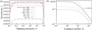
Growth rate of the leading quasi-stationary
 $(S_{\unicode[STIX]{x1D706}}=0)$
mode computed with various number of collocation points
 $M$
and Fourier modes
 $N$
versus the mapping parameter
 $\unicode[STIX]{x1D6FC}$
(a); growth rates of the three leading modes versus the Lundquist number computed with
 $M=64$
,
 $N=4096$
,
 $\unicode[STIX]{x1D6FC}=0.3$
(b).

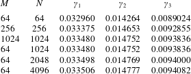
Growth rates of the three leading quasi-stationary
 $(S_{\unicode[STIX]{x1D706}}=0)$
modes computed with various number collocation points
 $M$
, Fourier modes
 $N$
and
 $\unicode[STIX]{x1D6FC}=0.3$
.

5 Results
We start with the quasi-stationary limit, which corresponds to
 $S_{\unicode[STIX]{x1D706}}=0$
, and first verify the accuracy of our numerical method. The highest growth rate
 $\unicode[STIX]{x1D6FE}_{1}$
computed in this limit with various numbers of collocation points
 $M$
and Fourier modes
 $N$
is plotted in figure 2(a) against the mapping parameter
 $\unicode[STIX]{x1D6FC}$
. First, note that
 $\unicode[STIX]{x1D6FE}_{1}$
is real and positive, which means a monotonic instability. The same holds also for the two subsequent eigenvalues shown in table 1, which are several times smaller than
 $\unicode[STIX]{x1D6FE}_{1}$
. Second, the growth rate is seen to be nearly constant over a wide range of the mapping parameter
 $\unicode[STIX]{x1D6FC}$
. For
 $M=64$
collocation points, a noticeable variation, which is a purely numerical effect, appears only for
 $\unicode[STIX]{x1D6FC}\lesssim 10^{-2}$
and
 $\unicode[STIX]{x1D6FC}\gtrsim 10$
. The growth rate computed with
 $M=64$
is nearly constant almost over three decades of
 $\unicode[STIX]{x1D6FC}$
. As seen in figure 2, the range of constant
 $\unicode[STIX]{x1D6FE}_{1}$
extends over more than five decades of
 $\unicode[STIX]{x1D6FC}$
when
 $M\geqslant 256$
. In the following, we fix
 $\unicode[STIX]{x1D6FC}=0.3$
, which is close to the centre of this range. Then
 $M=64$
produces
 $\unicode[STIX]{x1D6FE}_{1}$
coinciding up four decimal places with the value computed with
 $M=1024$
, which is a typically fast convergence of the Chebyshev collocation approximation. The convergence, however, is much slower with respect to the number of Fourier modes
 $N$
. As seen in table 1,
 $N\gtrsim 1024$
is required to compute the leading eigenvalue
 $\unicode[STIX]{x1D6FE}_{1}\approx 0.0335$
with 4 decimal places. Convergence is presumably slowed down by the edge singularity, which is discussed below, as well as by the discontinuity of the scalar magnetic potential over the current sheet resulting from the boundary condition (2.10). This discontinuity limits the Fourier series convergence rate to algebraic while the convergence rate of the Chebyshev collocation approximation is typically exponential (Gottlieb & Orszag Reference Gottlieb and Orszag1977). Further, we use
 $N=4096$
and
 $M=64$
.
Growth rates of the three leading modes computed using the full dynamical model (3.11), (3.12) are plotted in figure 2(b) versus the Lundquist number
 $S_{\unicode[STIX]{x1D706}}$
. For
 $S_{\unicode[STIX]{x1D706}}\ll 1$
, the quasi-stationary limit considered above is obviously recovered. As
 $S_{\unicode[STIX]{x1D706}}$
increases, the development of instability is slowed down by the increasing magnetic diffusion time. For
 $S_{\unicode[STIX]{x1D706}}\gtrsim 10$
, the growth rate is seen to reduce as
 $\unicode[STIX]{x1D6FE}\sim S_{\unicode[STIX]{x1D706}}^{-1}$
, which confirms the asymptotics inferred in § 3. The asymptotic growth rate of the dominant mode
 $\unicode[STIX]{x1D6FE}\sim 0.325/S_{\unicode[STIX]{x1D706}}$
is seen to agree well with the prediction of the reduced dynamical model for ideally conducting liquid described in the previous section.
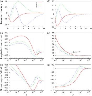
Amplitude distributions of the transverse velocity
 $\hat{v}$
(a,b), the longitudinal current density
 $-{\hat{h}}^{\prime }$
(c,d) and the normal magnetic field
 $\hat{B}$
(e,f) for the three fastest growing modes in the quasi-stationary (a,c,e) and ideally conducting (b,d,f) limits. The amplitudes are normalized by the condition
 $\hat{v}^{\prime }(0)=-1$
. The normal magnetic field in the ideally conducting case is rescaled with
 $(2\unicode[STIX]{x03C0}\unicode[STIX]{x1D6FE}S_{\unicode[STIX]{x1D706}}^{2})^{-1}$
so that
 $\hat{B}(0)=\hat{v}^{\prime }(0)$
.

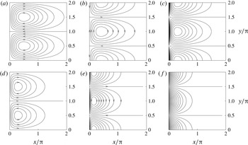
Streamlines (a,d), electric current lines (b,e) and the normal magnetic field isolines (c,f) of the fastest growing mode in the quasi-stationary (a,b,c) and ideally conducting (d,e,f) limits.

Amplitude distributions of the three fastest growing modes in both poorly and ideally conducting limits are plotted versus the distance from the edge in figure 3. The fastest growing mode, whose streamlines are shown in figure 4(a,b), is seen to have a single row of recirculation cells along the edge. Figure 3(a,b) shows that each subsequent mode has one more row of cells, which are separated by the zero crossings of
 $\hat{v}$
. The perturbation of the normal magnetic field in the quasi-stationary limit, which is shown in figure 3(e), has a characteristic logarithmic singularity similar to that of the base field (2.1). This singularity is presumably behind the slow convergence noted above. As seen in figure 3(f), this singularity vanishes in the ideally conducting limit. For a negligible magnetic diffusion, equation (3.12) at the edge
 $(x\rightarrow 0)$
reduces to
 $\unicode[STIX]{x1D6FE}S_{\unicode[STIX]{x1D706}}^{2}\hat{B}(0)=\hat{v}^{\prime }(0)/2\unicode[STIX]{x03C0}$
, which implies a finite normal magnetic field
 $\hat{B}(0)$
proportional to the longitudinal velocity
 $\hat{u} (0)=i\hat{v}^{\prime }(0)$
along the edge. But this, in turn, means a singularity in the longitudinal current density, which is seen in figure 3(d) to increase as
 ${\sim}x^{-1/2}$
towards the edge. Such a singular current distribution is typical at the edges of perfectly conducting sheets, where it generates a purely tangential magnetic field (Priede, Etay & Fautrelle Reference Priede, Etay and Fautrelle2006; Priede Reference Priede2011). The current singularity is obviously smoothed out by finite magnetic diffusion, which thus produces a normal magnetic field through the sheet with a logarithmic singularity at the edge. The associated spatial amplitude distribution of the scalar magnetic potential
 $\hat{\unicode[STIX]{x1D6F9}}(x,z)$
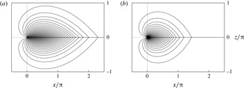
may be seen in figure 5 to have a symmetric discontinuity over the sheet with a continuous normal derivative which defines the normal magnetic field through the sheet. In the ideally conducting limit shown in figure 5(b), the perturbation is entirely due to the advection of the magnetic field and, thus, more localized at the edge. In the quasi-stationary limit shown in figure 5(a), the perturbation is spread out over the sheet by the magnetic diffusion.
Amplitude distributions of the scalar magnetic potential perturbation
 $\hat{\unicode[STIX]{x1D6F9}}$
in the
 $(x,z)$
-plane at the edge of sheet for the fastest growing mode in the quasi-stationary (a) and ideally conducting (b) limits.

As may be seen in figure 3, the increased current density at the edge is produced by the flow towards the edge. It means that the flow effectively compresses the current lines where it is directed towards the edge, while the opposite is the case where the flow is directed away from the edge. As this happens between the vortices, the associated pattern of current lines in figure 4(d,e) is shifted by a quarter wavelength relative to the streamline pattern in figure 4(a,d).
The compression of the current lines occurs as follows. According to (2.7), a flow in a non-uniform magnetic field induces electric current in order to conserve the magnetic flux carried by the liquid. Since the magnetic field drops off with the distance from the edge, the flow towards the edge locally reduces the magnetic flux density, which may be seen in figure 3(f) for the perfectly conducting limit. This, in turn, implies an increase in the current density at the edge. The current density at the edge has to raise in order to compensate the magnetic field generated by the rest of the sheet. The increased local current density interacting with the base magnetic field enhances the pinch force. This effect outweighs the advection of weaker magnetic field towards the edge. As a result, the initial flow perturbation towards the edge is enhanced, thus giving rise to instability in ideally conducting liquid.
Additional amplification of the instability results from the magnetic diffusion, which, as discussed above, smooths out the current singularity, so producing a logarithmic singularity in the normal magnetic field at the edge. As seen in figure 3(e), this perturbation is positive and, thus, enhancing the base field at the edge. Therefore, the growth rate of instability increases as the magnetic diffusion becomes stronger and the Lundquist number respectively smaller. As seen in figure 2(b), the growth rate saturates at
 $S_{\unicode[STIX]{x1D706}}\lesssim 10$
, which means that the instability becomes dominated by the magnetic diffusion. In this range of
 $S_{\unicode[STIX]{x1D706}}$
, the instability grows on the magnetic response time scale (3.9), which by a factor of
 $S_{\unicode[STIX]{x1D706}}^{-1}$
exceeds the respective Alfvén time scale (3.13). The latter is seen to apply only to
 $S_{\unicode[STIX]{x1D706}}\gtrsim 10$
.
6 Summary and conclusions
In this study, we considered a pinch-type instability in a semi-infinite planar sheet of an inviscid incompressible liquid with a straight rigid edge carrying a uniform tangential electric current. The electromagnetic pinch force resulting from the interaction of the electric current with its own magnetic in this model is balanced by the pressure gradient in quiescent liquid. This equilibrium state was found to be inherently unstable with respect to the internal flow perturbation caused by a row of counter-rotating vortices along the edge. The vortices compress the electric current lines where the flow is directed towards the edge and disperse them in the opposite case. The compression and dispersion of the current lines occurs as a weaker magnetic field is advected by the flow towards the edge and a stronger field is carried away. The interaction of the current perturbation with the base magnetic field produces a pinch force that amplifies initial flow perturbation. In an ideally conducting liquid, this part of the pinch force dominates over the opposing one which results from the interaction of the magnetic flux perturbation with the base current.
The role of the latter changes in the resistive limit, where it becomes destabilizing and dominant. The difference in the instability mechanism is due to the current and the magnetic field distributions at the edge. In an ideally conducting liquid, perturbation of the magnetic field remains finite at the edge, whereas the associated current density increases as
 ${\sim}x^{-1/2}$
becoming unbounded at the edge. In a resistive liquid, this current singularity is smoothed out by the magnetic diffusion, which thus produces a logarithmic singularity in the magnetic field. The latter enhances the base magnetic field at the edge. This gives rise to a destabilizing perturbation of the pinch force which dominates in the highly resistive liquid over the interaction of the current perturbation with the base magnetic field.
Different instability mechanisms lead to disparate instability development times in the highly resistive and well conducting fluids. In the former, the instability develops on the magnetic response time scale, which depends on the conductivity. In the latter, the instability develops on the much shorter Alfvén time scale. This is because the perturbation of the magnetic field in poorly conducting fluid depends on the product of conductivity and velocity, whereas in well conducting fluid the magnetic field is effectively frozen in and, thus, its perturbation depends directly on the displacement. Therefore these two instability development times are generic and, thus, expected to hold also in other geometries with fixed boundaries regardless of singularities in the magnetic field or the electric current distributions.
It follows from our model that the relevant electromagnetic parameter of the problem is the linear current density. In the eutectic alloy of GaInSn with
 $\unicode[STIX]{x1D70C}=6.4\times 10^{3}~\text{kg}~\text{m}^{-3}$
and
 $\unicode[STIX]{x1D70E}=3.3\times 10^{6}~\text{S}~\text{m}^{-1}$
(Weber et al.
Reference Weber, Galindo, Stefani, Weier and Wondrak2013) carrying linear current density of
 $J_{0}=1~\text{kA}~\text{cm}^{-1}$
, which is comparable to the respective quantity for the
 $m=1$
instability mode in the cylinder with the radius of 5 cm and the critical current of 2.9 kA (Rüdiger, Schultz & Gellert Reference Rüdiger, Schultz and Gellert2011; Seilmayer et al.
Reference Seilmayer, Stefani, Gundrum, Weier, Gerbeth, Gellert and Rüdiger2012), the characteristic instability development time is
 $\unicode[STIX]{x1D70F}_{m}/\unicode[STIX]{x1D6FE}_{1}\approx 30\unicode[STIX]{x1D70C}/(\unicode[STIX]{x1D70E}\unicode[STIX]{x1D707}_{0}^{2}J_{0}^{2})\approx 4~\text{s}$
, where
 $\unicode[STIX]{x1D6FE}_{1}\approx 0.0335$
is the dimensionless growth rate of the most unstable resistive mode. Note that in a Li–Te liquid-metal battery, where the areal current density can reach up to
 $j_{0}=7~\text{A}~\text{cm}^{-2}$
(Kim et al.
Reference Kim, Boysen, Newhouse, Spatocco, Chung, Burke, Bradwell, Jiang, Tomaszowska and Wang2013), the linear current density
 $J_{0}=1~\text{kA}~\text{cm}^{-1}$
corresponds to a layer of thickness
 $\unicode[STIX]{x1D6FF}\sim 1~\text{m}$
. The respective instability development time in Li (
 $\unicode[STIX]{x1D70E}=3.3\times 10^{6}~\text{S}~\text{m}^{-1}$
,
 $\unicode[STIX]{x1D70C}=0.5\times 10^{3}~\text{kg}~\text{m}^{-3}$
) (Müller & Bühler Reference Müller and Bühler2001) is then by an order of magnitude shorter than that in GaInSn. Comparing the instability development time in GaInSn with the viscous damping time
 $\unicode[STIX]{x1D70F}_{\unicode[STIX]{x1D708}}=\unicode[STIX]{x1D6FF}^{2}/12\unicode[STIX]{x1D708}$
due to the kinematic viscosity
 $\unicode[STIX]{x1D708}$
in the respective Hele-Shaw flow (Batchelor Reference Batchelor1967), we can estimate the critical Hartmann number
 $\mathit{Ha}_{c}=\unicode[STIX]{x1D707}_{0}J_{0}\unicode[STIX]{x1D6FF}\sqrt{\unicode[STIX]{x1D70E}/\unicode[STIX]{x1D70C}\unicode[STIX]{x1D708}}=\sqrt{12/\unicode[STIX]{x1D6FE}_{1}}\approx 20$
. This value is comparable with
 $\mathit{Ha}_{c}\approx 25$
for the non-axisymmetric
 $(m=1)$
instability mode in the cylindrical geometry (Rüdiger et al.
Reference Rüdiger, Schultz and Gellert2011), and it is also not far from
 $\mathit{Ha}_{c}\approx 40$
for the axisymmetric mode in the annular geometry (Priede Reference Priede2015). For
 $\mathit{Ha}\gtrsim 10$
, a more adequate estimate may be provided by the so-called Hartmann damping time
 $\unicode[STIX]{x1D70F}_{H}=(\unicode[STIX]{x1D6FF}^{2}/2\unicode[STIX]{x1D708})\,\mathit{Ha}^{-1}$
(Sommeria & Moreau Reference Sommeria and Moreau1982), which is based on the Hartmann rather than Poiseuille velocity profile, as in the Hele-Show flow, and yields
 $\mathit{Ha}_{c}=2/\unicode[STIX]{x1D6FE}_{1}\approx 60$
. For liquid metals, which are relatively poor conductors characterized by a low magnetic Prandtl number
 $\mathit{Pm}=\unicode[STIX]{x1D707}_{0}\unicode[STIX]{x1D70E}\unicode[STIX]{x1D708}\sim 10^{-5}{-}10^{-6}$
, all these critical Hartmann numbers
 ${\sim}10$
correspond to the Lundquist number
 $S_{\unicode[STIX]{x1D706}}=\mathit{Ha}\mathit{Pm}^{1/2}\lesssim 0.1$
, which means a highly resistive mode of instability.
In conclusion, note that in a viscous fluid, the threshold of instability, which is defined by
 $\unicode[STIX]{x1D6FE}=0$
, depends only on the Hartmann number (Rüdiger et al.
Reference Rüdiger, Schultz and Gellert2011). This is because the magnetic Prandtl number vanishes from (3.11) and (3.12) together with the Lundquist number similarly to the thermal Prandtl number in the case of Rayleigh–Bénard instability (Chandrasekhar Reference Chandrasekhar1961). But it is important to stress that the actual mechanism of the instability and, in particular, its growth rate depend on the Lundquist number. Also nonlinear evolution of the instability depends not on only on the Hartmann number but also on the Lundquist (magnetic Prandtl) number as recently demonstrated by Herreman et al. (Reference Herreman, Nore, Cappanera and Guermond2015).
Acknowledgements
This work was supported by Helmholtz Association of German Research Centres (HGF) in the framework of the LIMTECH Alliance through an agreement between Coventry University and Helmholtz–Zentrum Dresden–Rossendorf.