





1. Introduction
The head-on collision between a deformable liquid droplet and a bubble constitutes one of the canonical free-boundary problems in multiphase fluid mechanics, involving the coupled effects of interfacial hydrodynamics, capillary dynamics and singular free-surface motion (Manga & Stone Reference Manga and Stone1994; Eggers & Villermaux Reference Eggers and Villermaux2008; Prosperetti & Tryggvason Reference Prosperetti and Tryggvason2009; Deike Reference Deike2022; Balachandar Reference Balachandar2024). Unlike collisions of rigid particles, the interfaces separating the immiscible phases are not known a priori but evolve as part of the solution through the nonlinear coupling between the Navier–Stokes equations and the interfacial boundary conditions. Each interface is advected by the local velocity through the kinematic condition while reshaping the surrounding flow through the Young–Laplace pressure jump and the tangential-stress balance. Velocity, pressure and interface geometry therefore constitute a fully coupled moving-boundary problem in which deformation continuously alters the stresses that drive further deformation, admitting no fixed hierarchy of dominant forces.
Even the seemingly simple interaction of a single droplet with a single bubble exhibits a remarkable sequence of coupled hydrodynamic processes, including interface flattening, lubrication-film drainage, pressure amplification, vorticity generation, capillary-wave propagation, liquid-sheet formation, jet ejection and ultimately leading to rebound, attachment, coalescence, penetration or fragmentation (Manga & Stone Reference Manga and Stone1994; Thoroddsen et al. Reference Thoroddsen, Takehara, Nguyen and Etoh2018a ; Deike Reference Deike2022). These outcomes emerge from a competition between inertia, viscosity, capillarity and liquid-film drainage whose relative importance shifts continuously during impact. As the interfaces approach, the intervening liquid is expelled through an increasingly thin lubrication film; the resulting hydrodynamic pressure resists further approach and redistributes momentum within both phases, while inertia promotes deformation and flow focusing and surface tension opposes any increase in interfacial area. Because the lubrication pressure depends sensitively on an interface geometry that itself evolves under that pressure, no single asymptotic description captures the entire process.
The problem is also intrinsically multiscale. The droplet radius sets the outer scale for global momentum transport, whereas the lubrication film thins by several orders of magnitude before rupture or rebound, and the inertial, viscous, capillary and drainage time scales are often comparable. Vorticity is generated at the deforming interfaces by two mechanisms: baroclinic torque from the misalignment of density and pressure gradients across the capillary jump, and viscous generation through the tangential-stress balance (Batchelor Reference Batchelor1967; Prosperetti & Tryggvason Reference Prosperetti and Tryggvason2009). The resulting vortical structures redistribute momentum, modify the transient pressure field and thereby regulate deformation, pressure focusing and jet formation. When inertia dominates capillary restoring forces, convergence towards the symmetry axis produces a high-speed Worthington-type jet whose velocity can exceed the impact velocity and pierce the opposing interface or trigger fragmentation (Thoroddsen et al. Reference Thoroddsen, Takehara, Nguyen and Etoh2018a ; Deike Reference Deike2022).
The same mechanisms underpin many natural and engineering systems across a wide range of scales. Bubble-mediated droplet capture is the basis of mineral flotation, dissolved-air flotation, wastewater treatment, aeration and bubble-column reactors, where collision efficiency controls process performance (Bai et al. Reference Bai, Wang and Tu2011; Piccioli et al. Reference Piccioli, Aanesen, Zhao, Dudek and Øye2020; Abdal et al. Reference Abdal, Kahouadji, Shin, Chergui, Juric, Caulfield and Matar2024). Related interfacial interactions arise in spray combustion, cloud microphysics, emulsification, subsea oil dispersion and ocean–atmosphere gas exchange (Poo & Ashgriz Reference Poo and Ashgriz1991; Qian & Law Reference Qian and Law1997; Zhao et al. Reference Zhao, Boufadel, King, Robinson, Gao, Socolofsky and Lee2017; Li et al. Reference Li, An, Gao, Zhao and Sun2018). Despite differing widely in material properties, length scales and operating conditions, these systems share the same nonlinear interplay of inertia, capillarity, viscosity and interfacial topology. Therefore, understanding droplet–bubble collisions provides a building block for models of many-body interactions, dense dispersions and turbulent multiphase flows.
Schematic of the computational configuration for the head-on collision between an oil droplet moving towards the right (yellow in colour) and an air bubble moving towards the left (blue in colour) immersed in an otherwise quiescent liquid. The droplet and bubble move towards each other with equal and opposite velocities of magnitude
 $V_0$
and are separated by an initial gap
 $h$
. The computational domain has dimensions
 $L\times H\times H$
, with droplet and bubble diameters of
 $2a$
and
 $2\Delta a$
, respectively. The grey plane denotes the central meridional section used for flow visualisation, together with a magnified view of the local mesh near the interfaces. The coordinate system is also indicated. The fully three-dimensional computational domain contains approximately
 $10^9$
hexahedral control volumes.

Typical applications involving droplet–bubble collisions in various air-flotation and natural processes. Thermophysical properties and dimensionless numbers for bubble, droplet and surrounding liquid are listed. Non-bold values are from references, while bold values are estimated from classical formulae (see § 2 for scales). Our work is inspired by applications 5 and 6. Note that in application 4, the high gas density results from compression at a depth of approximately 1500 m, whereas the oil density changes only marginally because of its weak compressibility.

Table 1. Long description
Panel A: Table with six applications involving droplet-bubble collisions. Columns include application descriptions, density (kg/m3), kinematic viscosity (m2/s), size range (m), Reynolds number range, and Weber number range for bubble, droplet, and liquid. Panel B: Detailed values for each application, with non-bold values from references and bold values estimated from classical formulae. Applications range from water treatment to oil-water separation and subsea blowouts.
We investigate the head-on collision of a liquid droplet of radius
 $a$
, density
 $\rho _d$
and dynamic viscosity
 $\mu _d$
with a bubble of radius
 $\Delta \,a$
, density
 $\rho _b$
and dynamic viscosity
 $\mu _b$
(figure 1), both suspended in an otherwise quiescent liquid of density
 $\rho _l$
and dynamic viscosity
 $\mu _l$
. The droplet–liquid surface tension is
 $\sigma _{\mathrm dl}$
and the initial approach speed is
 $V_0$
. The parameter space is characterised by three dimensionless groups,
 \begin{align} \textit{Re} =\frac {2\rho _d aV_0}{\mu _d}, \qquad \textit{We}=\frac {2\rho _d aV_0^2}{\sigma _{\mathrm dl}}, \qquad \textit{Oh}=\frac {\mu _d}{\sqrt {2\rho _da\sigma _{\mathrm dl}}}, \end{align}
the ratios of inertial to viscous (
 $ \textit{Re}$
for Reynolds number), inertial to capillary (
 $ \textit{We}$
for Weber number) and viscous to inertial–capillary (
 $ \textit{Oh}$
for Ohnesorge number) forces, respectively. Only two are independent since
 $ \textit{Re}=\sqrt {\textit{We}}/\textit{Oh}$
. The surrounding liquid and gas enter through the density ratios
 $\rho _d/\rho _l$
,
 $\rho _b/\rho _l$
and viscosity ratios
 $\mu _d/\mu _l$
,
 $\mu _b/\mu _l$
, held fixed at values representative of millimetric gas–liquid systems. Table 1 collects representative physical and dynamical parameters for such systems; the spread of densities, viscosities and sizes yields a broad range of
 $ \textit{Re}$
and
 $ \textit{We}$
associated with distinct deformation, drainage, coalescence and breakup behaviours. In the relatively low-inertia flotation systems represented by applications 1–3, the bubbles are typically within the micrometre range and the corresponding bubble Reynolds and Weber numbers remain small, indicating that viscous and surface-tension forces dominate the interfacial dynamics. Application 4 represents droplet and bubble formation during subsea blowouts, where bubbles and droplets can reach millimetre-to-centimetre length scales and experience Reynolds numbers of
 $\mathcal{O}(10^{2}$
–
 $10^{3})$
and Weber numbers of
 $\mathcal{O}(10^{1}$
–
 $10^{2})$
. The relatively high gas density of
 $135\,\mathrm{kg\,m^{-3}}$
in application 4 corresponds to a pressurised gas phase at a depth of about
 $1500\,\mathrm{m}$
. In contrast, oil droplets are only weakly compressible and therefore remain in the liquid state; consequently, even under high hydrostatic pressures, their density increases only marginally and remains close to its ambient value. Application 5 considers subsurface oil releases and covers a broad range of droplet sizes, Reynolds numbers and Weber numbers, extending from weakly inertial, nearly spherical droplets to strongly deformable droplets that may undergo stretching and breakup. Application 6 describes oil–water separation in a cyclonic flotation column, where the high rotational liquid velocity produces Reynolds numbers of approximately
 $500$
,
 $1000$
and
 $1400$
for the bubble, droplet and surrounding liquid, respectively, together with bubble and droplet Weber numbers extending up to
 $\mathcal{O}(10^{3})$
and
 $\mathcal{O}(10^{2})$
. This regime is therefore characterised by strong inertia, appreciable interface deformation and possible fragmentation.
Whether attachment is thermodynamically favourable is determined independently of the flow by the spreading coefficient,
 $S=\sigma _{bl}-\sigma _{\mathrm dl}-\sigma _{db}$
, where
 $\sigma _{bl}$
,
 $\sigma _{\mathrm dl}$
and
 $\sigma _{db}$
denote the bubble–liquid, droplet–liquid and droplet–bubble interfacial tensions, respectively (Grattoni et al. Reference Grattoni, Moosai and Dawe2003). A positive value of
 $S$
favours complete wetting of the bubble by the droplet. In the present study, however, we restrict attention to
 $S\lt 0$
, for which spreading is energetically unfavourable and the collision outcome is governed primarily by transient hydrodynamics rather than equilibrium energetics. Experiments under steady collision conditions show that attachment occurs only when the thermodynamic criterion is satisfied and the intervening liquid film drains sufficiently rapidly before the interfaces separate (Yan et al. Reference Yan, Yang, Bai, Xu and Wang2020, Reference Yan, Zhang, Yang and Huang2021, Reference Yan, Zhang, Peng, Yang, Huang, Bai and Xu2022). If the intervening film reaches a critical thickness, it ruptures, allowing the interfaces to attach or coalesce. Otherwise, the lubrication pressure generated within the film counteracts the relative motion, inhibits further approach and induces droplet rebound. Since the approach velocity strongly influences drainage through interface deformation and the resulting transient pressure field (Yang et al. Reference Yang, Li, Tang, Hu, Zhang, Liu and Deen2025), the outcome cannot be inferred from equilibrium energetics alone.
At small Weber numbers, the interfaces remain nearly spherical, and the interaction is governed primarily by lubrication forces and viscous dissipation. Increasing
 $ \textit{We}$
drives dimple formation, asymmetric pressure fields, internal circulation and, above a threshold, axial jets that may pierce the opposing interface (Nguyen Reference Nguyen1999; Ray et al. Reference Ray, Biswas and Sharma2012, Reference Ray, Biswas and Sharma2015; Thoroddsen et al. Reference Thoroddsen, Takehara, Nguyen and Etoh2018b
; Roy et al. Reference Roy, Sophia and Basu2023; Sommer et al. Reference Sommer, Heitkam and Eckert2024). Experiments and direct numerical simulation (DNS) have documented these transitions and mapped their dependence on impact velocity, fluid properties and wettability, but almost exclusively for binary droplet collisions. Work addressing the droplet–bubble configuration directly is comparatively sparse and has concentrated on the near-contact and attachment stage (Nguyen Reference Nguyen1999; Yan et al. Reference Yan, Yang, Bai, Xu and Wang2020, Reference Yan, Zhang, Yang and Huang2021, Reference Yan, Zhang, Peng, Yang, Huang, Bai and Xu2022; Sommer et al. Reference Sommer, Heitkam and Eckert2024), establishing when contact and attachment occur while leaving the inertia-dominated, jet-forming stage, and the transient pressure and vortex fields that produce it, largely unexplored. For droplet–bubble collisions it remains unresolved how the impact conditions are transformed into the transient hydrodynamic structures that select the final state: no predictive framework connects the impact inertia to pressure focusing, interfacial vorticity generation and liquid-jet formation, which limits our ability to anticipate rebound, attachment, penetration or fragmentation. Surfactants complicate this further, since non-uniform coverage produces Marangoni stresses that oppose film thinning and interface stretching, alter interface mobility, delay jetting and can render the critical Weber number non-monotonic in concentration (Zhao et al. Reference Zhao, Zhang, Xu, Li and Liu2016; Antonopoulou et al. Reference Antonopoulou, Harlen, Rump, Segers and Walkley2021; Pico et al. Reference Pico, Kahouadji, Shin, Chergui, Juric and Matar2024); we exclude them here to isolate the intrinsic hydrodynamics. Table 1 places representative systems in this landscape, from low-inertia flotation devices with
 $ \textit{Re},\textit{We}=\mathcal{O}(1)$
, where drainage dominates, to millimetric droplets in oil-dispersion and separation devices with
 $ \textit{Re}$
up to
 $\mathcal{O}(10^{2})$
–
 $\mathcal{O}(10^{5})$
and
 $ \textit{We}=\mathcal{O}(10)$
–
 $\mathcal{O}(10^{2})$
, where inertia drives deformation, pressure concentration and jetting.
Three questions motivate this study. First, how does the radius ratio
 $\varDelta$
alter the impact dynamics? The curvature mismatch redistributes the impact pressure and reorganises the interfacial vorticity, yet its effect on the impulsive deceleration of the droplet and the efficiency of axial pressure focusing has not been established systematically. Second, what mechanism governs liquid-jet formation after impact? Internal jetting in droplet impact, cavity and bubble collapse and wave focusing arises when localised pressure amplification converts distributed kinetic energy into concentrated axial motion (Thoroddsen et al. Reference Thoroddsen, Thoraval, Takehara and Etoh2011; Ray et al. Reference Ray, Biswas and Sharma2012, Reference Ray, Biswas and Sharma2015; Thoroddsen et al. Reference Thoroddsen, Takehara, Nguyen and Etoh2018b
; van Rijn et al. Reference van Rijn, Westerweel, van Brummen, Antkowiak and Bonn2021); whether the same pressure-impulse mechanism operates here, and how the jet velocity relates to the transient pressure, interface curvature and vortex evolution, is unknown. Third, can physically grounded scaling laws relate the impact-induced pressure amplification and jet velocity to the governing dimensionless groups and thereby predict the transitions between regimes?
We address these questions with DNS of head-on droplet–bubble collisions in a quiescent liquid, using a volume-of-fluid formulation that resolves the large interfacial deformation together with the transient pressure and internal flow. The configuration is surfactant-free with
 $S\lt 0$
, so the dynamics reflects only the competition among inertia, viscosity, capillarity and pressure-driven momentum transport, free of turbulence, many-body interactions and Marangoni effects. To separate the universal early-time response from genuinely nonlinear finite-inertia dynamics, we adopt the unsteady motion of a nearly spherical, weakly deforming droplet as the reference solution. The point at which the numerical solutions depart systematically from this reference marks the onset of finite-inertia deformation. This complements our recent analysis of internal jetting in a single impulsively driven droplet (Senapati et al. Reference Senapati, Singh, Atta and Lakkaraju2025). Here, the two deforming interfaces, their curvature mismatch and the intervening liquid-film drainage introduce coupled dynamics absent from the single-droplet problem. We vary
 $ \textit{We}$
and
 $\varDelta$
across the inertia-dominated range relevant to millimetric gas–liquid systems and diagnose each collision through the transient interface, pressure, velocity and vorticity fields together with a budget of kinetic energy, surface energy and dissipation.
The remainder of the paper is organised as follows. Section 2 presents the governing equations, the numerical methodology and the validation. Section 3 presents the DNS of droplet–bubble collisions over a broad range of Weber numbers and size ratios. The collision dynamics is first characterised, after which the transient droplet motion is interpreted using the classical theory for unsteady droplet translation and compared with the numerical simulations. Section 4 develops scaling laws for the jet velocity by combining impulsive drag and pressure amplification, and validates the resulting predictions against the DNS. Section 5 summarises the conclusions and the perspectives for future work.
2. Problem formulation, governing equations and numerical methods
We consider the transient head-on collision of a spherical oil droplet of radius
 $a$
with a spherical air bubble of radius
 $\Delta a$
immersed in an otherwise quiescent viscous liquid (figure 1). Initially, the two interfaces are separated by a distance
 $h$
and approach each other with equal and opposite velocities of magnitude
 $V_0$
, giving a relative impact velocity of
 $2V_0$
. The dynamics is governed by the coupled evolution of momentum transport, interfacial deformation, capillary stresses and viscous dissipation arising from the interaction of the two deformable interfaces. The governing parameter space is explored by systematically varying the impact velocity
 $V_0$
, the bubble-to-droplet size ratio
 $\varDelta$
and the relevant thermophysical properties of the three-phase system.
The oil droplet, surrounding liquid and air bubble are modelled as incompressible, immiscible continua. Their evolution is governed by the incompressible Navier–Stokes equations, which are solved using the volume-of-fluid method (Wardle & Weller Reference Wardle and Weller2013; Shonibare & Wardle Reference Shonibare and Wardle2015; Dritselis & Karapetsas Reference Dritselis and Karapetsas2022) implemented in OpenFOAM 10 (Greenshields et al. Reference Greenshields2015) through the multiphaseInterFoam solver (Deshpande et al. Reference Deshpande, Trujillo and Kim2013; Senapati et al. Reference Senapati, Singh and Lakkaraju2019, Reference Senapati, Singh, Atta and Lakkaraju2025). Whereas our companion study (Senapati et al. Reference Senapati, Singh, Atta and Lakkaraju2025) examined the deformation and transient jetting of an isolated impulsively accelerated droplet, the present work addresses the fundamentally more complex two-interface interaction between a droplet and a bubble. The additional degrees of freedom introduced by the deformable bubble give rise to coupled interface dynamics, momentum exchange and transient energy redistribution that ultimately determine the collision regimes, jet formation and force decomposition analysed in the subsequent sections.
Each phase carries a volume fraction
 $\alpha _i$
(
 $i=b,d,l$
for bubble, droplet, liquid) subject to
 $\sum _i\alpha _{i}=1$
. Mass and momentum conservation are
 \begin{align} \boldsymbol{\nabla }\boldsymbol{\cdot }\boldsymbol{u} &= 0, \\[-12pt] \nonumber \end{align}
 \begin{align} {\frac {\partial (\rho \boldsymbol{u})}{\partial t} } +\boldsymbol{\nabla }\boldsymbol{\cdot }(\rho \boldsymbol{u}\boldsymbol{u}) &= -\boldsymbol{\nabla }{p}+\boldsymbol{\nabla }\boldsymbol{\cdot } \big[\mu \big(\boldsymbol{\nabla }\boldsymbol{u}+\boldsymbol{\nabla }\boldsymbol{u}^T \big) \big]+{f_s}, \\[10pt] \nonumber \end{align}
where
 $\boldsymbol{u}$
is the velocity,
 $p$
is the pressure,
 $\partial / \partial t$
is the partial time derivative,
 $\boldsymbol{\nabla}$
is the spatial gradient,
 $\boldsymbol{\cdot}$
is the inner product and superscript
 $T$
is the transpose operator. The mixture density
 $\rho =\sum _i\alpha _{i}\rho _{i}$
and the mixture dynamic viscosity
 ${\mu }=\sum _i\alpha _{i}\mu _{i}$
are computed using the volume-fraction fields. Interfacial tension is represented using the continuum surface force formulation (Brackbill et al. Reference Brackbill, Kothe and Zemach1992), which treats surface tension as a volumetric force distributed over the computational cells rather than acting solely at the interface. The generalisation of the continuum surface force in a three-phase system is modelled as
 $f_{s}=\sum _{i} \sum _{j\neq i} \sigma _{\textit{ij}} \kappa _{\textit{ij}}$
, where
 $\sigma _{\textit{ij}}$
is the interfacial tension coefficient between fluid
 $i$
and
 $j$
and
 $\kappa _{\textit{ij}} = -\boldsymbol{\nabla }\boldsymbol{\cdot }({\gamma _{\textit{ij}}/( |\gamma _{\textit{ij}}|+\epsilon )} )$
is the interfacial curvature computed using the indicator function
 $\gamma _{\textit{ij}} = \alpha _j \boldsymbol{\nabla }\alpha _{i} - \alpha _{i} \boldsymbol{\nabla }\alpha _j$
. Based on the computed interface normals, the local interface curvature is evaluated with a stabilisation parameter,
 $\epsilon$
, which accounts for the non-uniformity of the computational mesh. To represent the three-phase system, we employ an effective interfacial tension formulation that combines the phase-specific surface tension coefficients (Dritselis & Karapetsas Reference Dritselis and Karapetsas2022). The evolution of the volume fraction of each phase is then governed by the following equation:
 \begin{align} {\partial \alpha _i\over \partial t} + \boldsymbol{\nabla }\boldsymbol{\cdot }\left [\alpha _i\boldsymbol{u}- \sum _{{j\neq i}} \alpha _i \alpha _j \boldsymbol{u}_{r} \right ] = 0, \end{align}
where the artificial compression velocity
 $\boldsymbol{u}_{r}$
is used to sharpen the fluid interfaces (Senapati et al. Reference Senapati, Singh and Lakkaraju2019). To keep the volume fraction field bounded, we used the MULES (multidimensional universal limiter with explicit solution) method (Deshpande et al. Reference Deshpande, Anumolu and Trujillo2012; Damián & Nigro Reference Damián and Nigro2014).
The computational box has dimensions
 $L\times H\times H$
with
 $L=32a$
and
 $H=16a$
(Quan & Schmidt Reference Quan and Schmidt2006; Senapati et al. Reference Senapati, Singh, Atta and Lakkaraju2025). Finite-domain effects are negligible for this geometry because zero-Neumann velocity and constant atmospheric pressure are imposed at the boundaries (Senapati et al. Reference Senapati, Singh and Lakkaraju2019, Reference Senapati, Singh, Atta and Lakkaraju2025), as detailed in Appendix A. Each interface is treated as clean, with a constant surface-tension coefficient. The bubble is taken to be incompressible: for millimetric bubbles the deformation time scale far exceeds the internal pressure-equilibration time, the collision Mach number is
 $\ll 1$
and the deformation- and capillary-induced pressures are orders of magnitude below the ambient gas pressure. Bubbles therefore deform strongly while their volume remains essentially fixed, and the collision dynamics is governed by liquid inertia and capillarity. The unsteady flow in the surrounding liquid arises primarily from the impulsive motion of the droplet, whose density greatly exceeds that of the bubble. The
 $15$
governing dimensional variables (the three densities, three viscosities and three interfacial tensions, the impact speed
 $V_0$
, the droplet and bubble diameters, the initial gap
 $h$
and the domain dimensions
 $L,H$
) together with the three primary dimensions (mass, length, time) yield, by the Buckingham-
 $\pi$
theorem,
 $12$
independent dimensionless groups: the density ratios
 $\rho _b/\rho _d,\rho _l/\rho _d$
, the viscosity ratios
 $\mu _b/\mu _d,\mu _l/\mu _d$
, the interfacial-tension ratios
 $\sigma _{bl}/\sigma _{\mathrm dl},\sigma _{bd}/\sigma _{\mathrm dl}$
, the geometric ratios
 $\varDelta ,h/2a,L/2a,H/2a$
, and
 $ \textit{We}$
and
 $ \textit{Oh}$
. Holding the phase-property ratios fixed at the representative values of table 1 and the geometry and domain fixed, the collision dynamics is governed by the three control parameters
 $ \textit{We}$
,
 $ \textit{Oh}$
and
 $\varDelta$
, with
 $ \textit{Re}=\sqrt {\textit{We}}/\textit{Oh}$
following from these. Although the subsequent analysis relies primarily on physical scaling arguments rather than the non-dimensional governing equations, we present the latter in Appendix A for completeness.
Binary droplet studies in viscous oils show that the early approach is largely insensitive to the initial centroid separation, provided the bodies are initially placed between two and more diameters apart (Mohammadi et al. Reference Mohammadi, Shahhosseini and Bayat2012; Yuan et al. Reference Yuan, Dabirian, Shoham and Mohan2020). In this range, the interfaces are sufficiently separated to avoid immediate lubrication effects at the initial instant, while remaining close enough that the weak far-field hydrodynamic disturbance has a negligible influence on the subsequent evolution. Consequently, thin-film drainage, interfacial deformation and short-range hydrodynamic interactions develop only during the final stages of approach. We verified this for the present configuration using
 $h=3a$
,
 $3.5a$
and
 $4a$
, which gave nearly identical approach and collision characteristics, and we report the representative case
 $h=3.5a$
. Guided by the applications in table 1, we fix
 $\rho _l=2\rho _d$
,
 $\rho _b=0.002\rho _d$
and
 $\mu _l=2\mu _d$
, representative of aeration-based capture of oil droplets by bubbles (Grau et al. Reference Grau, Laskowski and Heiskanen2005; Saurel et al. Reference Saurel, Petitpas and Abgrall2008; Xu et al. Reference Xu, Liu, Li, Zhang and Wang2016; Balla et al. Reference Balla, Kavuri, Tripathi, Sahu and Govindarajan2020). This density ratio
 $\rho _l/\rho _d$
enters only through order-unity coefficients and does not alter the regime structure. In the droplet translation model developed in §§ 3 and 4, this parameter enters naturally through the added mass coefficient
 $\lambda ^{2}=9\rho _l/[\pi (2\rho _d+\rho _l)]$
; and the leading-order inertial balance gives the jet velocity
 $V_{\textit{jet}}/V_0\approx [(\rho _l/\rho _d)\varGamma _1]^{-1/2}$
, where
 $V_{\textit{jet}}$
is the maximum surrounding-liquid velocity and
 $\varGamma _1$
the jet-to-droplet volume ratio. For
 $\rho _l/\rho _d=2$
this reduces to
 $V_{\textit{jet}}/V_0\approx (2\varGamma _1)^{-1/2}$
, so the density ratio rescales only the
 $\mathcal{O}(1)$
prefactor while the scaling
 $V_{\textit{jet}}/V_0\propto \varGamma _1^{-1/2}$
and the boundaries set by
 $ \textit{We}$
,
 $ \textit{Oh}$
and
 $ \textit{Re}$
are unchanged. The same holds as
 $\rho _l/\rho _d\to 1$
, since both ratios are
 $\mathcal{O}(1)$
and introduce no new dominant force.
The governing equations are discretised by the finite-volume method, with the intermediate velocity advanced by the Pressure-Implicit with Splitting of Operators (PISO) algorithm (Ma et al. Reference Ma, Liu, Zu and Tang2012): a pressure-correction step enforces mass conservation, after which the transport equation for
 $\alpha _i$
is solved. Time integration uses the first-order implicit Euler scheme and the spatial fluxes a total-variation-diminishing scheme with the van Leer limiter (Sweby Reference Sweby1984). On the hexahedral mesh the time step (
 $\Delta t$
) is kept far below the capillary time
 $t_c=\sqrt {\rho _d(2a)^3/8\sigma _{\mathrm dl}}$
(specifically
 $\Delta t/t_c\approx 1.2\times 10^{-2}$
), and the Courant number below
 $0.2$
. The simulations are performed in Cartesian coordinates
 $(x,y,z)$
, whereas the analysis uses spherical coordinates
 $(r,\theta ,\phi )$
attached to the instantaneous droplet centroid moving at
 $V_0$
, related by the standard transformations. Figure 2 validates the solver against experiment (Qian & Law Reference Qian and Law1997) and simulation (Chen et al. Reference Chen, Khare and Yang2011) for a binary droplet collision in air. Further details of the numerical methodology, numerical validation and grid convergence are provided in the supplementary material available at https://doi.org/10.1017/jfm.2026.12200. In particular, the supplementary material presents a mesh sensitivity analysis of the droplet–bubble thin-film drainage by examining the convergence of the minimum film thickness and the relative approach velocity, thereby establishing the adequacy of the adopted computational resolution for the macroscopic drainage dynamics considered here.
Validation and grid convergence study for the head-on collision of two tetradecane droplets in air at
 $ \textit{We}=61.4$
and
 $ \textit{Oh}=0.026$
. Numerical results obtained using two mesh resolutions,
 $\Delta x=a/50$
and
 $\Delta x=a/60$
, are compared with the experimental observations of Qian & Law (Reference Qian and Law1997) and the numerical simulations of Chen et al. (Reference Chen, Khare and Yang2011). The excellent agreement demonstrates the ability of the present numerical methodology to accurately capture the collision dynamics and confirms that the adopted mesh provides grid-independent predictions for the macroscopic interfacial evolution. Permission to reproduce the comparison data has been requested from the respective copyright holders.

3. Flow features during unsteady motion of a droplet and a bubble
When a droplet or bubble is impulsively set into motion, unsteady effects dominate the initial dynamics. The surrounding liquid responds only gradually, so a mismatch between inertia and viscous diffusion produces transient added-mass forces and a developing boundary layer. Sharp interfacial velocity gradients feed shear layers that roll up into vortices, controlling the drag and the unsteady wake and, when strong enough, driving asymmetric motion and breakup. At early times the Basset history force adds a further unsteady drag from accumulated vorticity (Leal Reference Leal2007), which is most important at low
 $ \textit{Oh}$
, where it couples strongly to interface deformability. Unlike rigid spheres, droplets and bubbles also oscillate in shape, and these oscillations interact with the surrounding vorticity to modify the local stresses. Because droplet inertia dominates, we first characterise the flow generated by an impulsively driven droplet and then analyse the droplet–bubble interaction.
Transient evolution of a suddenly decelerated isolated droplet translating from left to right in a quiescent viscous liquid. Four representative cases are shown: (a)
 $ \textit{We}=200$
,
 $ \textit{Oh}=1.11$
,
 $ \textit{Re}=12.74$
; (b)
 $ \textit{We}=200$
,
 $ \textit{Oh}=0.006$
,
 $ \textit{Re}=2357$
; (c)
 $ \textit{We}=35$
,
 $ \textit{Oh}=0.006$
,
 $ \textit{Re}=986$
; and (d)
 $ \textit{We}=13$
,
 $ \textit{Oh}=0.006$
,
 $ \textit{Re}=600$
. Time progresses from top to bottom in each column, corresponding to the non-dimensional times (in
 $V_0 t/(2a)$
) 3, 6 and 12. In every snapshot, the upper half shows the normalised pressure field, while the lower half presents the velocity vectors together with the normalised streamwise velocity magnitude in the surrounding liquid. The same linear colour scale, ranging from
 $-0.5$
(blue) to
 $0.5$
(red), is used for both the pressure and velocity fields. Although the simulations are fully three-dimensional, only the central meridional plane is shown to illustrate the evolution of the pressure field, wake structure and jet formation more clearly.

3.1. Decelerating droplet in a viscous liquid
The unsteady motion of a single droplet in a quiescent viscous liquid sets the baseline for its subsequent interaction with a bubble. An impulsively driven droplet, decelerating under viscous resistance, generates flow structures governed by the interplay of inertia, viscosity and capillarity and characterised by
 $ \textit{We}$
and
 $ \textit{Oh}$
. Figure 3 shows snapshots of the interface, the normalised pressure field and the mid-plane liquid velocity at three instants, revealing the coupling between interfacial deformation and the surrounding flow.
For high
 $ \textit{Oh}\gt 1$
, the dynamics enters a viscosity-dominated regime in which momentum diffusion occurs more rapidly than inertial interface deformation. The translational kinetic energy is dissipated continuously through viscous stresses rather than being redirected into capillary deformation. As a result, the rear interface remains smooth, no dimple or jet develops and the droplet approaches the equilibrium spherical state at long times despite the imposed pressure gradient (figure 3
a). Deformation stays weak, axisymmetry is preserved and the response is set by the balance between viscous stress and surface tension rather than inertia. For low
 $ \textit{Oh}\ll 1$
, inertial effects dominate the droplet response. The rear interface develops a dimple, which subsequently focuses into a liquid jet as the imposed pressure gradient accelerates the fluid. At high inertia (
 $ \textit{We}=200$
,
 $ \textit{Oh}=0.006$
) the droplet transfers substantial kinetic energy to the liquid, and the rearward jet elongates until it ruptures the interface into a three-dimensional toroidal shape. At moderate inertia (
 $ \textit{We}=35$
) the jet cannot pierce the interface and the droplet remains a prolate ellipsoid with a shallow dimple, reflecting an inertial–capillary balance. At low inertia (
 $ \textit{We}=13$
) deformation is weak and nearly axisymmetric, dominated by linear modes. In every case a toroidal vortex ring develops behind the droplet, coupled to the streamwise pressure gradient and the elongation. These results demonstrate that
 $ \textit{We}$
and
 $ \textit{Oh}$
are the primary parameters governing droplet deformation.
Flow regime map for head-on droplet–bubble collisions in the
 $(We,\varDelta )$
parameter space for
 $ \textit{Oh}=0.006$
. More than 100 three-dimensional simulations were performed to identify four distinct collision regimes, denoted by circles (Regime I), diamonds (Regime II), triangles (Regime III) and squares (Regime IV). Representative interface evolutions are shown alongside the regime map. Regime I (
 $ \textit{We}=13$
,
 $ \textit{Re}=600$
,
 $\varDelta =1$
) results in attachment without jet formation. Regime II (
 $ \textit{We}=70$
,
 $ \textit{Re}=1394$
,
 $\varDelta =0.5$
) exhibits secondary droplet formation without attachment. Regime III (
 $ \textit{We}=70$
,
 $ \textit{Re}=1394$
,
 $\varDelta =1$
) is characterised by jet-induced attachment. Regime IV (
 $ \textit{We}=200$
,
 $ \textit{Re}=2357$
,
 $\varDelta =1$
) produces strong jet stretching followed by interface separation. The regime map highlights the combined influence of impact inertia and bubble size ratio on the transition between attachment, jet formation and breakup. The droplet (moving to the right) is shown in yellow and the bubble (moving to the left) in blue.

Regime I for droplet–bubble collision for
 $ \textit{We}=13$
,
 $ \textit{Oh} = 0.006$
,
 $ \textit{Re} = 600$
and
 $\varDelta =1$
. Attachment is observed with time. In each snapshot, the top half is for normalised pressure and the bottom half for velocity vectors with streamwise velocity (in magnitude and normalised with
 $V_0$
) in the surrounding liquid. Colourbar consists of linear scale from blue (−0.5 value) to red (0.5 value), and the same combination and range are used for both the pressure and the velocity. Droplet in yellow and bubble in blue. Animation is available at Animation-1.

Regime II for droplet–bubble collision for
 $ \textit{We}=70$
,
 $ \textit{Oh} = 0.006$
,
 $ \textit{Re} = 1394$
and
 $\varDelta =0.5$
. Secondary droplet generates with time, but no attachment is observed. In each snapshot, the top half is for normalised pressure and the bottom half for velocity vectors with streamwise velocity (in magnitude and normalised with
 $V_0$
) in the surrounding liquid. Colourbar consists of linear scale from blue (−0.5 value) to red (0.5 value), and the same combination and range are used for both the pressure and the velocity. Droplet in yellow and bubble in blue. Animation is available at Animation-2.

3.2. Droplet collision with a bubble
Based on the single-droplet dynamics, we now examine droplet–bubble collisions in the viscous medium. Simulations span
 $3\lt We\lt 270$
,
 $289 \lt Re\lt 2739$
,
 $0.5\le \varDelta \le 2$
and
 $ \textit{Oh}=0.006$
. Although the initial
 $ \textit{Re}$
is large, the droplet decelerates rapidly, so the instantaneous
 $ \textit{Re}$
falls quickly; the small
 $ \textit{Oh}$
keeps viscous damping weak, so the response is set by rapid interfacial motion rather than viscous diffusion, and jet-induced deformations develop clearly enough to classify. Unlike binary droplet collisions in a gas (Nikolopoulos et al. Reference Nikolopoulos, Nikas and Bergeles2009; Chen et al. Reference Chen, Khare and Yang2011), droplet motion in a liquid host drives strong rearward jets through a persistent low-pressure wake. Figure 4 maps the parameter space into four regimes.
In Regime I (
 $ \textit{We}\le 20$
,
 $0.5\le \varDelta \le 2$
; figure 5), the droplet collides and gradually attaches to form a single coupled unit; toroidal vortices and streamwise pressure variations accompany oscillations between dimpled (concave) and bulged (convex) shapes before attachment. In Regime II (
 $30\le We\lt 80$
,
 $0.5\le \varDelta \le 0.8$
; figure 6), the jet penetrates the primary droplet and ejects a satellite droplet that attaches to the bubble, following oscillatory deformation, jet narrowing and lateral displacement of the bubble and satellite. Finally, the primary droplet does not get attached to the bubble. In Regime III (from
 $ \textit{We}\approx 30$
,
 $\varDelta =2$
to
 $ \textit{We}\approx 250$
,
 $\varDelta =0.5$
; figure 7), a conical jet penetrates the droplet but, unlike Regime II, causes no secondary breakup; the entire droplet becomes a toroidal ring that merges with the bubble into a coherent coupled unit. In Regime IV (
 $ \textit{We}\gt 250$
for
 $\varDelta =0.5$
,
 $ \textit{We}\gt 120$
for
 $\varDelta =2$
; figure 8), strong jetting drives a combined toroidal droplet–bubble attachment: the jet pierces both the droplet and the bubble interior, both elongate into toroids and secondary droplets form. The maximum droplet elongation reaches about three times its initial diameter, consistent with binary-droplet studies (Al-Dirawi et al. Reference Al-Dirawi, Al-Ghaithi, Sykes, Castrejon-Pita and Bayly2021) (supplementary material, figure S12).
Regime III for droplet–bubble collision for
 $ \textit{We}=70$
,
 $ \textit{Oh} = 0.006$
,
 $ \textit{Re} = 1394$
and
 $\varDelta =1$
. Jet induced droplet–bubble attachment with time. In each snapshot, the top half is for normalised pressure and the bottom half for velocity vectors with streamwise velocity (in magnitude and normalised with
 $V_0$
) in the surrounding liquid. Colourbar consists of linear scale from blue (−0.5 value) to red (0.5 value), and the same combination and range are used for both the pressure and the velocity. Droplet in yellow and bubble in blue. Animation is available at Animation-3.

Regime IV for droplet–bubble collision for
 $ \textit{We}=200$
,
 $ \textit{Oh} = 0.006$
,
 $ \textit{Re} = 2357$
and
 $\varDelta =1$
. Jet stretching and separation with time (the reader is referred to Appendix S10 of the supplementary material for more details). In each snapshot, the top half is for normalised pressure and the bottom half for velocity vectors with streamwise velocity (in magnitude and normalised with
 $V_0$
) in the surrounding liquid. Colourbar consists of linear scale from blue (−0.5 value) to red (0.5 value), and the same combination and range are used for both the pressure and the velocity. Droplet in yellow and bubble in blue. Animation is available at Animation-4.

Figure 8. Long description
Panel A: A heat map showing the interaction between a droplet and a bubble at t = 0.3a/V0. The top half represents normalized pressure, and the bottom half shows velocity vectors with streamwise velocity in the surrounding liquid. The color scale ranges from blue (0.5 value) to red (0.5 value). The droplet is yellow, and the bubble is blue. Panel B: A heat map showing the interaction at t = 3a/V0. The top half represents normalized pressure, and the bottom half shows velocity vectors with streamwise velocity in the surrounding liquid. The color scale ranges from blue (0.5 value) to red (0.5 value). The droplet is yellow, and the bubble is blue. Panel C: A heat map showing the interaction at t = 6a/V0. The top half represents normalized pressure, and the bottom half shows velocity vectors with streamwise velocity in the surrounding liquid. The color scale ranges from blue (0.5 value) to red (0.5 value). The droplet is yellow, and the bubble is blue. Panel D: A heat map showing the interaction at t = 10a/V0. The top half represents normalized pressure, and the bottom half shows velocity vectors with streamwise velocity in the surrounding liquid. The color scale ranges from blue (0.5 value) to red (0.5 value). The droplet is yellow, and the bubble is blue. Panel E: A heat map showing the interaction at t = 24a/V0. The top half represents normalized pressure, and the bottom half shows velocity vectors with streamwise velocity in the surrounding liquid. The color scale ranges from blue (0.5 value) to red (0.5 value). The droplet is yellow, and the bubble is blue. Panel F: A heat map showing the interaction at t = 100a/V0. The top half represents normalized pressure, and the bottom half shows velocity vectors with streamwise velocity in the surrounding liquid. The color scale ranges from blue (0.5 value) to red (0.5 value). The droplet is yellow, and the bubble is blue.
These transitions demonstrate that the collision outcome is governed by the coupled effects of impact inertia and the bubble-to-droplet-size ratio. For low inertia, capillary restoration dominates and stable attachment occurs in Regime I. As the impact inertia increases, the liquid jet acquires sufficient momentum to generate secondary droplets without attachment of the primary droplet in Regime II. With a further increase in inertia, the jet and the accompanying toroidal vortex become the dominant transport mechanisms, producing increasingly strong interface deformation and giving rise to Regimes III and IV. The collision regime is therefore selected by the competition between capillary restoration and the persistence of the jet vortex system. The collision thus progresses from quasi-linear, capillary-controlled motion to strongly nonlinear jet-induced morphologies, showing the role of inertial penetration in restructuring and coupling liquid–gas interfaces.
3.3. Unsteady effects around an impulsively driven droplet
At low
 $ \textit{We}$
the droplet translates as a nearly spherical body with weak, dimple-free deformation and little jetting, and the unsteady translation of a weakly deforming droplet provides a well-defined reference for the collision dynamics. The recirculation and incipient jet seen once inertia grows originate in unsteady effects and the diffusion of vorticity from the droplet surface into the liquid (Maxey & Riley Reference Maxey and Riley1983; Auton et al. Reference Auton, Hunt and Prud’Homme1988; Magnaudet & Mougin Reference Magnaudet and Mougin2007). To quantify this early-time response, we estimate the relevant time scales, the unsteady drag and the droplet speed under the Oseen approximation for a rigid sphere.
The unsteady Oseen approximation (Pearcey & Hill Reference Pearcey and Hill1956; Bentwich & Miloh Reference Bentwich and Miloh1978; Leal Reference Leal2007; Simeonov Reference Simeonov2015) describes the transient motion of a suddenly accelerated, spherical body in an otherwise quiescent fluid by extending the Stokes solution to include the leading-order convective inertial correction. Although it is traditionally formulated for small but finite Reynolds numbers, it isolates the roles of unsteady inertia, added mass and history effects in setting the transient drag, wake development and particle transport. In the present problem the initial Reynolds number
 $ \textit{Re}=2\rho _d a V_0/\mu _d$
is large, but the impulsively driven droplet decelerates rapidly, so the instantaneous value
 $ \textit{Re}(\mathsf{t})=2\rho _d a V(\mathsf{t})/\mu _d$
, with
 $ \textit{Re}(0)=Re$
, falls continuously from the outset. We therefore employ the unsteady Oseen solution not as a description of the complete flow but as a reduced model of the early-time force balance. The convective term enters only to close the quasi-steady drag, contributing a bounded
 $\mathcal{O}(1)$
correction. When expressed in the viscous time
 $\mathsf{t}=\pi \nu _l\lambda ^2 t/a^2$
, with
 $\lambda ^2=9\rho _l/[\pi (2\rho _d+\rho _l)]$
, the velocity evolution collapses to a one-parameter family depending only on
 $\mathsf{a}=\lambda \sqrt {\pi }$
(we explain it in a later part of the section). The accuracy of the reduced model is therefore closely correlated with the extent of interfacial deformation. Since the droplet deformation is initially negligible, the weak-deformation approximation is asymptotically valid as
 $\mathsf{t}\rightarrow 0$
for all
 $ \textit{Oh}$
considered here. The subsequent departure from the DNS coincides with the onset of appreciable finite-inertia deformation, suggesting that interfacial deformation is an important contributor to the loss of agreement. However, since the present cases also involve finite Reynolds numbers and the effects of Reynolds number and deformation are not independently separated, finite-
 $ \textit{Re}$
effects may also contribute to the observed departure.
For completeness and to make the underlying force balance transparent, we briefly revisit the classical derivation in the laboratory frame, where the disturbance velocity vanishes and the pressure approaches its ambient value in the far field. We define the Oseen Reynolds number of the surrounding liquid as
 $ \textit{Re}_O = 2 V_0 a/\nu _l$
, related to the droplet Reynolds number through
 $ \textit{Re}_O = (\rho _l/\rho _d)(\mu _d/\mu _l)\,Re$
, so that
 $ \textit{Re}_O = Re$
for the ratios adopted here. The near field,
 $r \ll L_O$
with Oseen length
 $L_O \sim 2a/Re_O$
, is viscous, and the Stokes drag
 $6\pi \mu _l a V_0$
of a nearly spherical droplet holds there, whereas convective corrections dominate the far field,
 $r \gg L_O$
, where the inertial asymmetry of the wake gives the
 $ \textit{Re}_O$
-dependent form
 $6\pi \mu _l a V_0\,[\,1+ ({3}/{8})Re_O+\cdots \,]$
, which is not uniformly valid near the surface. A logarithmic intermediate region provides the overlap between the two limits. In the unsteady problem the short-time response is diffusion-controlled, while the long-time response reflects the gradual emergence of inertia and the wake, and we solve the resulting equations in the Laplace domain and invert them to obtain the flow and force histories across this transition.
The unsteady Oseen approximation for the axisymmetric, viscous flow around a spherical droplet, an assumption justified in the limit of small Weber numbers, can be recast, upon linearising the convective term, in terms of the vorticity field
 $\boldsymbol{\zeta }=\boldsymbol{\nabla }\times \boldsymbol{u}$
as
 \begin{align} \left [\frac {\partial }{\partial t}+V_0\frac {\partial }{\partial x}-\nu _l{\nabla} ^{2}\right ]\boldsymbol{\zeta }=0, \end{align}
where the axisymmetric Laplacian is
 ${\nabla} ^{2}= [({1}/{r^{2}}) ({\partial }/{\partial r})] (r^{2} ({\partial }/{\partial r}) )+ [({1}/{r^{2}\sin \theta }) ({\partial }/{\partial \theta })] (\sin \theta \,({\partial }/{\partial \theta }) )$
, the streamwise derivative is
 $ {\partial }/{\partial x}=\cos \theta \, ({\partial }/{\partial r})- ({\sin \theta }/{r}) ({\partial }/{\partial \theta })$
and
 $ {\partial }/{\partial \phi }=0$
. For axisymmetric flow the only non-zero vorticity component is
 $\zeta _{\phi }$
, related to the Stokes streamfunction
 $\psi$
by
 $\zeta _{\phi }=- ({1}/{r\sin \theta }){\nabla} ^{2}\psi$
. Since the flow is independent of the azimuthal coordinate
 $\phi$
, the streamfunction depends only on
 $r$
,
 $\theta$
and time, so that
 $\psi =\psi (r,\theta ,t)$
. In the laboratory frame, a spherical droplet translates with velocity
 $V_{0}$
in the positive
 $x$
direction through an otherwise quiescent fluid, with the coordinate
 $\theta =0$
aligned with the direction of translation. The far-field condition is therefore
 $\boldsymbol{u}\to \boldsymbol{0}$
as
 $r\to \infty$
, while on the droplet surface the fluid velocity matches the prescribed translational motion. Using the standard transformations between Cartesian and spherical coordinates (Prosperetti Reference Prosperetti2011), the radial and tangential velocities in the surrounding liquid are
 \begin{align} u_r=\frac {1}{r^{2}\sin \theta }\frac {\partial \psi }{\partial \theta },\qquad u_\theta =-\frac {1}{r\sin \theta }\frac {\partial \psi }{\partial r}. \end{align}
The boundary conditions on the rigid droplet’s surface are as follows:
 \begin{align} u_r & = V_0\cos \theta ,\quad u_{\theta }=-V_0\, \sin\theta ,\quad r =a, \\[-12pt] \nonumber \end{align}
 \begin{align} u_{r} & = u_{\theta }=0, \qquad\qquad\qquad\qquad\quad r \to \infty . \\[10pt] \nonumber \end{align}
We decompose the streamfunction (Lamb Reference Lamb2002) into the irrotational field
 $\psi ^{(1)}$
and the solenoidal part
 $\psi ^{(2)}$
, to account for the impulse and the viscous effects, respectively, i.e.
 $\psi =\psi ^{(1)}+\psi ^{(2)}$
. By solving
 $\psi$
, the drag force can be solved as shown in Appendix A, which has the general form as
 \begin{align} \mathcal{D} &= 6\pi \rho _l\nu _l V_0 a \Biggl [ 1 + \frac {1}{\sqrt {\pi \tau }} - \frac {(1+\beta _1)\beta _1^{2}}{\sqrt {\pi }\,(\beta _1 - \beta _2)} {\rm e}^{-\beta _1^{2}\tau } \!\int _{0}^{\tau } \frac {{\rm e}^{\beta _1^{2}t}}{\sqrt {t}}\, {\mathrm dt} \nonumber \\[5pt]& +\, \frac {(1+\beta _2)\beta _2^{2}}{\sqrt {\pi }\,(\beta _1 - \beta _2)} {\rm e}^{-\beta _2^{2}\tau } \!\int _{0}^{\tau } \frac {{\rm e}^{\beta _2^{2}t}}{\sqrt {t}}\, {\mathrm dt} \Biggr ] +\, \frac {1}{2} M V_0\, \delta (\tau ), \end{align}
where
 $\tau ={\nu _l t/a^2}$
is the dimensionless viscous time scale,
 $M$
is the added mass,
 $\delta (\tau )$
is the Dirac delta function and
 $\beta _1$
and
 $\beta _2$
are the solutions of
 $80\beta ^2- ({V_0 a/ \nu _l} )^2\beta +4 ({V_0 a/ \nu _l} )^2=0$
.
At this level of approximation, the drag is a linear function of the instantaneous velocity, so continuously varying velocity histories follow by superposition. Decomposing the motion into infinitesimal velocity increments over successive intervals, the drag at any instant is the cumulative response to all prior increments, weighted by the fluid’s response function. This convolution form encodes the memory of unsteady viscous diffusion in the wake and is the familiar integral-kernel structure of unsteady Stokes and Oseen flow, as in the Basset–Boussinesq–Oseen equation (Leal Reference Leal2007). As a point-particle approximation, the total force on the droplet at time
 $t$
(for small
 $\tau$
) is
 \begin{align} \left (m+{1\over 2}M\right ){\mathrm dV_0\over {\mathrm dt}}+6\pi \rho _l\nu _l a V_0+{6\pi \rho _l\nu _l a^2 \over \sqrt {\pi \nu _l}}\int _0^{\infty }{1\over \sqrt {t'}}{\mathrm dV_0(t-t')\over {{\mathrm d}{t}'}}{{\mathrm d}{t}'}=\mathcal{F}, \end{align}
where the time integration is carried out from the start to an instantaneous time (
 $t=t'$
). The governing relation constitutes an integro-differential equation. In the absence of memory (Basset history) effects and external body forces (
 $\mathcal{F}$
), the evolution of the droplet velocity simplifies to an exponentially decaying form
 $ [({\mathrm dV_0/ {\mathrm dt})}\propto -V_0 ]$
, indicating the rapid dissipation of inertia through viscous diffusion. In contrast, when history effects are taken into account, the dynamics becomes more intricate with the velocity no longer following a simple exponential law, and instead the solution can be systematically expressed as a power-series expansion in time, capturing the gradual influence of the droplet’s past motion on its present evolution. The mentioned force equation is rescaled into dimensionless form by choosing appropriate scales as
 $m=({4/ 3})\pi \rho _d a^3$
,
 $M=({4/ 3})\pi \rho _l a^3$
(as an added-mass effect with appropriate 1/2 prefactor),
 $\mathsf{V}$
as normalised velocity,
 $\lambda ^2=9\rho _l/\pi (2\rho _d+\rho _l)$
and
 $\mathsf{t}=\pi \nu _l\lambda ^2 t/a^2$
. Thus we get the governing equation in rescaled form which is applicable for
 $\mathsf{t}\gt 0$
as
 \begin{align} \frac {\mathrm {d}\mathsf{V}}{{\mathrm {d}\mathsf{t}}} + \mathsf{V} + \lambda \int _0^{\infty } \frac {\textrm{d}{\mathsf{V}}(\mathsf{t} - \mathsf{t}')}{ {\rm d}(\mathsf{t} - \mathsf{t}')} \frac {\textrm{d} {\mathsf{t}}'}{\sqrt {\mathsf{t}'}} = 0. \end{align}
The unsteady added-mass and Basset (memory) contributions follow from the linearised dynamics and do not require a small Reynolds number; the convective (Oseen) linearisation enters only in closing the steady part of the drag, where it contributes a bounded
 $\mathcal{O}(1)$
correction. Retaining the leading dipole mode and neglecting the higher modes is thus justified in the spherical regime, which is the range over which (3.7) is compared with the simulations. Appendix A.1 provides a brief rederivation of the classical analytical solution for
 $\mathsf{V}(\mathsf{t})$
and summarises its early- and late-time asymptotic behaviour for the chosen initial condition.
Comparison between the analytical solution of (3.7) (a,b) and numerical simulations (c,d). (a) Evolution of the normalised drag, Basset history and inertia forces for
 $\lambda =0.5$
(solid) and
 $\lambda =2$
(dashed), as functions of the viscous diffusion time
 $(\pi \nu _l\lambda ^2/a^2)t$
. Increasing
 $\lambda$
strengthens the contribution of the Basset history force while maintaining the instantaneous force balance. (b) Corresponding evolution of the normalised droplet velocity,
 $V/V_0$
. (c) Normalised force balance from (3.6) by choosing DNS-based instantaneous droplet (centroid) velocity for
 $\lambda \approx 1.19$
. Continuous line for theory and dashed line for DNS data. (d) Analytical predictions from (3.6) (dashed) are compared with DNS (solid with markers) for different values of
 $ \textit{We}$
,
 $ \textit{Oh}$
and
 $\varDelta$
. Short- and long-time asymptotic limits shown in dash-dotted lines. Cases without
 $\varDelta$
correspond to an isolated droplet.

Figure 9(a) decomposes the analytical solution of (3.7) into its three constituent contributions: the quasi-steady drag
 $\mathsf{V}$
, the Basset history force proportional to the memory parameter
 $\lambda$
and the inertial contribution
 $\textrm{d}{\mathsf{V}}/\textrm{d}{\mathsf{t}}$
, which accounts for both droplet and added-mass inertia. Results are shown for two representative values,
 $\lambda =0.5$
and
 $2$
, and by construction the three terms satisfy the instantaneous force balance at every time. Immediately after release, the motion is governed almost entirely by a balance between quasi-steady drag and inertia. The drag assumes its maximum value,
 $\mathsf{V}=1$
, while the inertial term is nearly equal and opposite,
 $\textrm{d}{\mathsf{V}}/\textrm{d}{\mathsf{t}}\approx -1$
, reflecting the negligible influence of vorticity diffusion at very early times. As the surrounding vorticity field develops, the history force increases monotonically and overtakes the inertial contribution at
 $\mathsf{t}=O(1)$
, after which it becomes the dominant mechanism opposing the motion. At long times the inertial contribution decays most rapidly, as
 $\mathsf{t}^{-3/2}$
, whereas both the quasi-steady drag and the history force decay algebraically as
 $\mathsf{t}^{-1/2}$
and together govern the asymptotic relaxation. Increasing
 $\lambda$
amplifies the relative importance of the history force and consequently delays the decay of the velocity, as demonstrated in figure 9(b). The decomposition therefore identifies two distinct dynamical stages: an inertia-controlled initial response followed by a history-dominated viscous relaxation, with
 $\lambda$
governing the crossover between them.
Figure 9(c) compares the normalised force components reconstructed from the analytical solution of (3.7) (solid lines) with those obtained by substituting the instantaneous droplet-centroid velocity from the DNS into the corresponding quasi-steady drag, inertial and Basset history terms (dashed lines). This comparison provides a force-balance reconstruction based on the DNS centroid dynamics and demonstrates the consistency of the analytical force decomposition with the simulated droplet motion. The comparison is presented for the representative case
 $\lambda \approx 1.19$
,
 $ \textit{Oh}=0.84$
and
 $ \textit{We}=36$
, where viscous diffusion is sufficiently strong for memory effects to remain significant while finite inertial and deformation effects are present. Overall, the quasi-steady drag and inertial contributions exhibit good quantitative agreement over the entire time interval, demonstrating that the dominant momentum balance predicted by the analytical model is retained in the DNS. The Basset history force also captures the correct temporal evolution and asymptotic behaviour, although small quantitative differences emerge during the intermediate stage where the analytical model neglects finite-Reynolds-number effects, weak droplet deformation and other higher-order hydrodynamic interactions. Nevertheless, the comparison confirms that the history force remains an essential component of the momentum balance even at the relatively large Weber number considered, supporting the applicability of the analytical framework beyond the strictly creeping-flow limit.
Figure 9(d) compares the normalised droplet velocity obtained from the DNS with the analytical solution of (3.7), expressed in terms of the viscous diffusion time
 $\mathsf{t}=(\pi \nu _l\lambda ^2/a^2)t$
. The analytical solution (red dashed) connects smoothly the memory-free early-time behaviour,
 $V/V_0\simeq 1-\mathsf{t}$
, with the long-time algebraic decay,
 $V/V_0\sim \lambda \,\mathsf{t}^{-1/2}$
, which originates from the Basset history force. Expressed in this rescaled time, the evolution depends only upon the single parameter
 $\mathsf{a}=\lambda \sqrt {\pi }$
, yielding a universal velocity history for spherical, weakly deforming motion.
The DNS follows this analytical reference only while the interface remains approximately spherical. The duration of agreement is therefore governed primarily by the onset of finite deformation rather than by the Reynolds number. For the most viscous case,
 $ \textit{Oh}=0.84$
(
 $ \textit{We}=36$
), the numerical solution remains close to the analytical prediction until
 $\mathsf{t}=O(1)$
and approaches the algebraic asymptote. Similar agreement is obtained for
 $ \textit{Oh}=0.16$
(
 $ \textit{We}=6$
), where viscous damping suppresses shape oscillations and preserves an almost spherical interface. In contrast, at
 $ \textit{Oh}=0.006$
the agreement is restricted to the initial stage,
 $\mathsf{t}\lesssim 10^{-1}$
, during which deformation remains weak. The strongest inertial case,
 $ \textit{We}=70$
with
 $\varDelta =0.5$
, departs from the analytical solution first, coincident with the formation of the rear-interface dimple. Beyond these intervals the DNS develops oscillatory behaviour absent from the analytical solution, reflecting finite interfacial deformation, internal circulation, vortex–interface coupling and the onset of jet formation. The bubble-to-droplet size ratio
 $\varDelta$
modifies the detailed deceleration history through changes in momentum partition between the two phases, but does not alter the underlying sequence of physical mechanisms.
The comparison is not intended to validate the analytical solution over the entire parameter space. Instead, it provides a quantitative criterion for identifying the breakdown of the spherical, weakly deforming approximation. Equation (3.7) constitutes the classical solution of the governing free-boundary problem in this limit and serves as the hydrodynamic reference state against which the DNS is interpreted. As expected, it cannot capture the strongly nonlinear evolution of interface deformation, internal circulation, vortex generation, jet penetration and secondary-droplet formation that develops at finite Weber numbers. Its principal value lies in providing a parameter-free benchmark for the universal early-time response, so that the subsequent departure of the DNS from this reference quantitatively marks the emergence of finite-deformation dynamics. In this way, the classical unsteady-force theory is placed in direct correspondence with the fully nonlinear droplet–bubble collision dynamics examined in the present study.
4. Energy analysis in droplet–bubble interaction
As the droplet accelerates through the surrounding liquid, part of its kinetic energy is transferred to the fluid through unsteady inertial coupling, representable as an added-mass contribution. This coupling alters the droplet’s translation and drives localised flow focusing near its rear interface, forming a conical jet. The jet is a coherent, axisymmetric structure that penetrates the droplet in Regimes II–IV, and its formation is governed mainly by the exchange of kinetic and surface energies between droplet and liquid, with only a minor bubble contribution.
At the initial instant (
 $t = 0$
), both the droplet and the bubble possess nearly spherical shapes, and the total energy can be expressed as the sum of their kinetic and interfacial energies as
 \begin{align} \underbrace { \frac {1}{2}\rho _d \left (\frac {\pi }{6} d_{d_0}^3\right ) V_{d_0}^2 + \frac {1}{2}\rho _b \left (\frac {\pi }{6} d_{b_0}^3\right ) V_{b_0}^2 }_{\mathrm{initial\ kinetic\ energy}} \;+\; \underbrace { \sigma _{\mathrm dl}\,\pi d_{d_0}^2 + \sigma _{bl}\,\pi d_{b_0}^2 }_{\mathrm{initial\ surface\ energy}}. \end{align}
The interfacial tension coefficients are
 $\sigma _{\mathrm dl}$
(droplet–liquid) and
 $\sigma _{bl}$
(bubble–liquid). The use of diameters (
 $d_d$
,
 $d_b$
) instead of radii facilitates a consistent representation of both surface area and volume terms. The subscript ‘0’ refers to the initial configuration at
 $t=0$
.
To leading order, the total mechanical energy of the coupled system at a later time
 $t$
decomposes into the kinetic energy of the droplet centroid, the kinetic energy of the surrounding liquid (including added mass), the kinetic energy of the conical jet, the droplet and bubble surface energies and the viscous dissipation in the boundary layer:
 \begin{align} {1\over 2}\rho _d\left ({\pi \over 6}d^3_d\right )V^2_d + {1\over 2}\rho _l \forall_l V^2_l + {1\over 2}\rho _l \varGamma _1 \left ({\pi \over 6}d^3_{d0}\right ) V^2_{jet} & + \sigma _{\mathrm dl}\pi d^2_{d} + \sigma _{bl}\pi d^2_{b} \nonumber \\ & + \int _{0}^{t}\rho _l\nu _l \varGamma _2 {V_l^2 \over d^2_{d0}} \left ({\pi \over 6}d^3_{d0}\right )\, {\mathrm dt}. \end{align}
The jet kinetic energy is modelled as
 $ ({1}/{2})\rho _l\,\varGamma _1( ({\pi }/{6})d_{d0}^3)V_{\textit{jet}}^2$
, where
 $\varGamma _1(t)$
is the instantaneous jet volume normalised by the initial droplet volume. This captures the jet as an internal, axisymmetric structure whose volume grows as the interface deforms. Rapid droplet deformation, bubble collapse and interface focusing are known to produce slender conical jets (Gekle & Gordillo Reference Gekle and Gordillo2010); the early jet volume is negligible, motivating
 $\varGamma _1(0)=0$
, after which interface steepening yields an increasingly well-defined jet. The same phenomenology follows from rapid interfacial compression (Zeng et al. Reference Zeng, Zhang, Tan, An and Ohl2024), where pressure and curvature focusing generate a narrow, high-speed jet. The present jet-energy form is therefore consistent with the reported conical-jet geometry and effective volume.
As the droplet translates, it accelerates a finite region of ambient liquid, contributing a kinetic energy
 $ ({1}/{2})\rho _l\,\forall_l\,V_l^2$
, with
 $\forall_l$
the effective entrained volume. This follows from the classical added-mass formulation for accelerating bodies (Lamb Reference Lamb2002), in which surrounding fluid must be displaced before the body accelerates, raising its effective inertia (Batchelor Reference Batchelor1967). Since Magnaudet (Reference Magnaudet1997) showed that the hydrodynamic reaction depends sensitively on Reynolds number, interface deformability and wake structure, we do not fix
 $\forall_l$
at its inviscid value but treat it as an effective quantity reflecting the deformed surrounding flow.
Viscous stresses in the boundary layer around the droplet continuously remove mechanical energy. A leading-order estimate of the cumulative loss over
 $[0,t]$
is
 $\mathsf{E}_v \approx \int _{0}^{t}\rho _l\nu _l(V_l^2/d_{d0}^2)\,\varGamma _2(\pi d_{d0}^3/6)\, {\mathrm dt}$
, where
 $\varGamma _2$
corrects for the effective thickness and extent of the viscous region. The gradient estimate
 $V_l/d_{d0}$
follows from boundary-layer scaling, in which the near-surface velocity change scales as a characteristic velocity over the relevant length (Schlichting & Gersten Reference Schlichting and Gersten1999); Leal (Reference Leal2007) gives an explicit unsteady-flow dissipation that remains valid across a wide range of Reynolds numbers and deformation. Integrating to time
 $t$
completes the simplified energy budget. We retain only this outer boundary-layer dissipation and neglect the lubrication dissipation within the thin intervening film, which is asymptotically smaller during the inertia-dominated stage. With the outer strain rate set by the unsteady boundary layer of thickness
 $\delta \sim a\,Re^{-1/2}$
and the film thickness
 $h=\mathcal{O}(a)$
before drainage, the ratio of film to boundary-layer dissipation scales as
 $\varPhi _{{film}}/\varPhi _{{outer}}\sim (a_c/a)^2(\delta /h)=\mathcal{O}(Re^{-1/2})\ll 1$
for the present
 $ \textit{Re}=\mathcal{O}(10^2$
–
 $10^3)$
. Thin-film dissipation therefore enters only as a higher-order correction to (4.2) and becomes comparable with the outer loss only in the late-stage drainage regime (
 $h/a\ll 1$
), which lies outside the inertial balance considered here.
Figure 10(a) shows the individual energy components for
 $ \textit{We}=200$
. The droplet and bubble surface energies dominate the budget throughout, and the bubble kinetic energy is initially about three orders of magnitude below that of the droplet owing to its low density. The jet kinetic energy overtakes the droplet kinetic energy at
 $t\approx 2a/V_0$
. The shaded band marks the interval used to extract the jet velocity
 $V_{{jet}}$
, defined as the maximum surrounding-liquid velocity.
By enforcing conservation of total energy equating the initial energy in (4.1) to the energy at a later time in (4.2), and dividing both sides by the initial droplet surface energy, we obtain
 \begin{align} {\textit{We} \over 12} + \left ({\rho _b \over \rho _d}\right ) {\textit{We} \over 12} \varDelta ^3 + 1 +\left ({\sigma _{bl} \over \sigma _{\mathrm dl}}\right ) \varDelta ^2 & = {\textit{We} \over 12} \left (V_d \over V_0\right )^2 \left (a \over d_{d0}\right )^3 + \varGamma _1 { \textit{We} \over 12} \! \left ({\rho _l \over \rho _d}\right )\! \left (V_{jet} \over V_0\right )^2 \nonumber \\& \quad + \left (a \over d_{d0}\right )^2 + \left ({\sigma _{bl} \over \sigma _{\mathrm dl}}\right ) \left (d_b \over d_{b0}\right )^2 \varDelta ^2 \nonumber \\& \quad + {\textit{We} \over \pi } \left (V_l \over V_0\right )^2 \left ({{{\forall}}_l \over d^3_{d0}}\right ) \nonumber \\& \quad + \int _{0}^{t} \varGamma _2 \textit{Oh} \sqrt {\textit{We}} \left (V_l \over V_0\right )^2 \left (V_0 \over d_{d0}\right ) \left ({\rho _l\nu _l \over \rho _d\nu _d}\right )\, {\mathrm dt}. \end{align}
Equation (4.3) can be further rearranged to obtain the expression for
 $V_{jet}$
as
 \begin{eqnarray} \varGamma _1 { \textit{We} \over 12} \left ({\rho _l \over \rho _d}\right )\left (V_{jet} \over V_0\right )^2 & = & {\textit{We} \over 12} + \left ({\rho _b \over \rho _d}\right ) {\textit{We} \over 12} \varDelta ^3 + 1 +\left ({\sigma _{bl} \over \sigma _{\mathrm dl}}\right ) \varDelta ^2 - {\textit{We} \over 12} \! \left (V_d \over V_0\right )^2 \! \left (a \over d_{d0}\right )^3 \nonumber \\&& - \left (a \over d_{d0}\right )^2 - \left ({\sigma _{bl} \over \sigma _{\mathrm dl}}\right ) \left (d_b \over d_{d0}\right )^2 - {\textit{We} \over \pi } \left (V_l \over V_0\right )^2 {{{\forall}}_l \over d^3_{d0}} \nonumber \\&&- \int _{0}^{t} \varGamma _2 \textit{Oh} \sqrt {\textit{We}} \left (V_l \over V_0\right )^2 \left (V_0 \over d_{d0}\right ) \left ({\rho _l\nu _l \over \rho _d\nu _d}\right )\, {\mathrm dt}. \end{eqnarray}
Equation (4.4) can be rewritten in compact non-dimensional form as
 \begin{eqnarray} \frac {V_{jet}}{V_0} = \left [ \frac {12}{\varGamma _1 \textit{We}}\left (\frac {\rho _d}{\rho _l}\right ) (\mathfrak{A} - \mathfrak{K} - \mathcal{L} - \mathfrak{D})\right ]^{1/2}, \end{eqnarray}
where
 $\mathfrak{A} = ({1/ 12})\textit{We} + ( {\rho _b}/{\rho _d} )\ ({\textit{We}}/{12})\varDelta ^3 + 1 + ( {\sigma _{bl}}/{\sigma _{\mathrm dl}} )\varDelta ^2$
is the available initial energy (droplet inertia and interfacial),
 $\mathfrak{K} = ({1/ 12})\textit{We} ({V_d}/{V_0} )^2 ( {a}/{d_{d0}} )^3 + ( {a}/{d_{d0}} )^2 + ( {\sigma _{bl}}/{\sigma _{\mathrm dl}} ) ( {d_b}/{d_{d0}} )^2$
accounts for droplet and bubble kinetic energy corrections,
 $\mathcal{L} = ({1/ \pi })\textit{We} ({V_l}/{V_0} )^2 ({\forall_l}/{d_{d0}^3} )$
corresponds to bulk liquid motion and
 $\mathfrak{D} = \int _0^{t} \varGamma _2\, \textit{Oh} \sqrt {\textit{We}}({V_l}/{V_0} )^2 ({V_0}/{d_{d0}} ) ({\rho _l\nu _l}/{\rho _d\nu _d} ) \,{\mathrm dt}$
captures the cumulative viscous dissipation. This form identifies the jet velocity as the competition between available impact energy and the combined inertial and viscous losses.
For
 $ \textit{We}=200$
,
 $ \textit{Oh} = 0.006$
,
 $ \textit{Re} = 2357$
and
 $\varDelta =1$
in normalised coordinates: (a) energy versus time and (b) jet speed versus time. (a) Droplet surface energy (
 $\mathsf{S}_d$
), bubble surface energy (
 $\mathsf{S}_b$
), jet kinetic energy (
 $\mathsf{K}_{jet}$
), surrounding-liquid kinetic energy (
 $\mathsf{K}_{sl}$
), droplet kinetic energy (
 $\mathsf{K}_d$
), viscous energy dissipation (
 $\mathsf{E}_v$
) and bubble kinetic energy (
 $\mathsf{K}_b$
). (b) Jet speed estimation based on semi-analytical theory (in blue stars) and simulation (in red stars). The inset shows
 $\varGamma _1$
versus time. Snapshots for corresponding time (droplet in yellow and bubble in blue) and
 $\times$
mark at which the jet speed is computed.

Figure 10(b) compares the jet speed from the scaling theory and the simulations for
 $ \textit{We}=200$
. In the simulations we track the deforming droplet and measure the jet speed at the dimple (cross symbol); for the theory, the transient volume ratios and other quantities on the right-hand side of (4.4) are taken from the simulations, with
 $\varGamma _1\approx 1$
(see supplementary material, S12, for its dependence on
 $ \textit{We}$
and
 $\varDelta$
). Theory and simulation agree well for
 $t\gg a/V_0$
, indicating that in this unsteady problem the jet develops well beyond the viscous diffusion time. At early times (
 $t\ll a/V_0$
) the jet volume is negligible (
 $\varGamma _1\approx 0$
; inset of figure 10
b) and grows to
 $\mathcal{O}(1)$
for
 $t\gg a/V_0$
.
4.1. Inertial regime (
 $ \textit{We}\gg 1$
,
$ \textit{Oh}\ll 1$
)


When the Weber number is large and viscous effects are weak,
 $\mathfrak{A}\approx \textit{We}/12$
dominates, while
 $\mathfrak{K}$
,
 $\mathcal{L}$
and
 $\mathfrak{D}$
are of higher order. Equation (4.5) reduces to
 \begin{align} \frac {V_{jet}}{V_0} \approx \left [\left (\frac {\rho _l}{\rho _d}\right )\varGamma _1\right ]^{-1/2}=\sqrt {\frac {1}{2\varGamma _1}}\qquad (\rho _l=2\rho _d). \end{align}
The jet speed thus scales linearly with the impact speed and remains an
 $\mathcal{O}(1)$
fraction of
 $V_0$
, with a prefactor set mainly by the jet mass fraction
 $\varGamma _1$
; for
 $\varGamma _1\simeq 1$
,
 $V_{jet}\approx 0.7V_0$
. Equivalently, this is the leading balance between droplet impact energy and jet kinetic energy,
 $ (1/2)\rho _d(({\pi }/{6})d_d^3)V_0^2\simeq (1/2)\rho _l\varGamma _1(({\pi }/{6})d_{d0}^3)V_{jet}^2$
, giving
 $V_{jet}/V_0\simeq [(\rho _l/\rho _d)\varGamma _1]^{-1/2}$
directly; the density ratio enters only through the
 $\mathcal{O}(1)$
prefactor
 $(\rho _l/\rho _d)^{-1/2}$
, leaving the
 $\varGamma _1^{-1/2}$
scaling intact.
4.2. Capillary–inertial regime (
$ \textit{We}\ll 1$
,
$ \textit{Oh}\ll 1$
)


For weak impacts, the inertial term in (4.5) is small and the capillary term dominates the right-hand side. The scaling becomes
 \begin{align} V_{\textit{jet}}\sim \sqrt {{6\over \varGamma _1}\left (1+\mathcal{O}(\varDelta ^2)\right )\left (\frac {\sigma _{\mathrm dl}}{\rho _d d_{d0}}\right )}. \end{align}
In this limit the jet speed becomes independent of
 $V_0$
, controlled solely by the capillary–inertial velocity scale and geometrical factors (see Appendix S11 in the supplementary material for more on transient
 $V_{jet}$
profiles).
4.3. Viscous regime and critical limit
When viscous losses are significant, the dissipation term
 $\mathfrak{D}(t)\propto \varGamma _2 Oh\sqrt {\textit{We}}$
reduces the available energy for jet formation. A threshold for observable jetting occurs when
 $\varGamma _2\,Oh\sqrt {\textit{We}}\lesssim \mathcal{O}(1)$
, defining the critical Ohnesorge number
 $ \textit{Oh}_c \sim {C/\sqrt {\textit{We}}}$
, where
 $C$
is an
 $\mathcal{O}(1)$
constant related to
 $\varGamma _2$
and the interaction time. For the case shown in figure 10(a) (
 $ \textit{We}=200$
), this yields
 $ \textit{Oh}_c\simeq 0.07$
, consistent with the transition observed in simulations. For
 $ \textit{Oh}\ll Oh_c$
the system follows the inertia- or capillary-dominated scaling, whereas for
 $ \textit{Oh}\gtrsim Oh_c$
viscous dissipation suppresses the jet formation. In the intermediate regime,
 \begin{align} \frac {V_{\textit{jet}}}{V_0} \approx \sqrt {\left [ 1 - \textit{Oh}\,{\textit{We}}^{-1/2} \right ]}, \end{align}
with the gradual reduction of jet velocity with increasing viscosity. In Appendix S11 of the supplementary material, we present a comparison of the maximum values of
 ${V_{\textit{jet}}}/{V_0}$
obtained from the numerical and analytical results.
Asymptotic phase diagram of jetting regimes in the
 $(\textit{We},\textit{Oh})$
parameter space. The vertical line at
 $ \textit{We}\simeq 70$
separates the capillary-dominated and inertia-dominated regimes, while the curve
 $ \textit{Oh}_c\sim {\textit{We}}^{-1/2}$
denotes the critical Ohnesorge number above which viscous dissipation suppresses jet formation. Four asymptotic regimes are identified according to the dominant balance among inertia, capillarity and viscous dissipation. In the capillary regime,
 $V_{{jet}}\sim \sqrt {6\sigma _{\mathrm dl}/(2\varGamma _1\rho _da)}$
, whereas in the inertia-dominated regime,
 $V_{{jet}}/V_0\sim (2\varGamma _1)^{-1/2}$
.

Figure 11 summarises the asymptotic jetting regimes in the
 $(\textit{We},\textit{Oh})$
plane obtained from the leading-order balances of (4.4). Two boundaries emerge naturally: the vertical line
 $ \textit{We}\simeq 70$
, separating capillary- and inertia-dominated dynamics, and the critical curve
 $ \textit{Oh}_c\sim {\textit{We}}^{-1/2}$
, above which viscous dissipation suppresses jet formation. For
 $ \textit{We}\lt 70$
and
 $ \textit{Oh}\lt Oh_c$
, the jet velocity is governed by the capillary–inertial scale,
 $ V_{{jet}}\sim \sqrt {6\sigma _{\mathrm dl}/(2\varGamma _1\rho _d a)}$
, and is essentially independent of the impact speed. For
 $ \textit{We}\gt 70$
and
 $ \textit{Oh}\lt Oh_c$
, inertia dominates the energy conversion, giving
 $ V_{{jet}}/V_0\sim (2\varGamma _1)^{-1/2}$
, so that the jet remains an
 $\mathcal{O}(V_0)$
fraction of the impact velocity. For
 $ \textit{Oh}\gt Oh_c$
, viscous dissipation progressively extracts the available kinetic energy, leading to viscous–capillary and viscous–inertial regimes in which jet formation is increasingly attenuated.
These asymptotic regimes provide a unified interpretation of the numerical observations. Inertia initially transfers translational kinetic energy into interface deformation and subsequently into the focused liquid jet, whereas capillarity restores the interface and viscosity irreversibly dissipates energy. The transition at
 $ \textit{We}\simeq 70$
marks the onset of efficient inertial focusing, while the critical scaling
 $ \textit{Oh}_c\sim {\textit{We}}^{-1/2}$
quantifies the competition between inertial energy input and viscous dissipation. Since
 $\rho _b/\rho _d\ll 1$
, the bubble contributes negligibly to the kinetic energy budget, and the impact energy is transferred predominantly into liquid acceleration and surface deformation. The size ratio
 $\varDelta$
enters the reduced description through the geometric factor
 $\varGamma _1$
, which accounts for the geometric contribution to the energy focusing. Within the range of
 $\varDelta$
and
 $ \textit{We}$
investigated here, however,
 $\varGamma _1$
exhibits only modest case-to-case variations, with no discernible systematic dependence on either parameter (reported in the supplementary material). Thus, while
 $\varGamma _1$
sets the prefactor associated with energy focusing in the reduced model, the dominant balance and the resulting asymptotic jetting regime are primarily determined by
 $ \textit{We}$
and
 $ \textit{Oh}$
.
5. Summary and discussion
We have investigated head-on droplet–bubble collisions in a quiescent, surfactant-free liquid using three-dimensional volume-of-fluid DNS over a broad range of bubble-to-droplet size ratios (
 $0.5\le \varDelta \le 2$
), Weber numbers (
 $3\le \textit{We}\le 270$
) and small Ohnesorge numbers (
 $ \textit{Oh}\lt 1$
). By isolating a single pairwise interaction, the present study eliminates the additional complexity associated with turbulence, surfactants and many-body interactions, thereby exposing the elementary hydrodynamic and interfacial mechanisms that govern droplet–bubble encounters. These pairwise interactions constitute the fundamental building blocks of flotation, aeration, emulsification and liquid–liquid separation processes.
The simulations reveal that the collision dynamics is organised by the competition between inertia, capillarity, viscous diffusion and interfacial mobility. Four distinct collision regimes emerge, ranging from smooth oscillatory attachment at weak inertia to jet-mediated penetration, toroidal deformation and secondary-droplet formation at increasingly larger Weber numbers. A robust transition from capillary-controlled to inertia-dominated dynamics occurs near
 $ \textit{We}\approx 23$
, largely independent of the bubble-to-droplet size ratio, whereas the onset of complete jet penetration depends strongly on
 $\varDelta$
. These results demonstrate that the Weber number governs the initial loss of spherical behaviour, while the size ratio controls the subsequent evolution of the coupled interfaces once large deformations develop.
To interpret the weakly deforming limit, we compare the DNS with the analytical solution of the classical unsteady history-force model for an impulsively accelerated spherical droplet, which incorporates added-mass effects together with the Basset memory force. The analytical solution recovers the bounded early-time deceleration and the inverse-square-root velocity decay associated with viscous diffusion of vorticity. The agreement with the DNS persists only while the interface remains nearly spherical. As the Weber number increases, the numerical solution departs progressively from the analytical prediction owing to the onset of finite interfacial deformation, internal recirculation, vortex–interface coupling and jet formation. Rather than viewing this departure as a limitation of the reduced model, we exploit it as a quantitative diagnostic of the breakdown of spherical dynamics. The analytical solution therefore provides a hydrodynamic reference state that enables the onset of nonlinear free-boundary effects to be identified directly from the simulations.
An energy-based analysis further clarifies the physical origin of jet formation. At low Weber numbers, the impact energy is stored predominantly as surface energy and subsequently released through capillary oscillations, preventing jet formation. As inertia increases, the conversion of translational kinetic energy into localised interfacial motion produces a focused liquid jet, whose characteristic velocity scales as
 $V_{{jet}}\sim V_0/\sqrt {2\varGamma _1}$
for
 $\varGamma _1=\mathcal{O}(1)$
. Viscous dissipation limits this focusing mechanism, leading to the critical scaling
 $ \textit{Oh}_c\sim We^{-1/2}$
beyond which high-speed jetting is progressively suppressed. These results identify the energetic pathway through which impact inertia is redistributed into deformation, vortex generation and secondary atomisation.
The present study is intentionally restricted to idealised pairwise collisions between a clean droplet and a clean bubble in an otherwise quiescent liquid. Consequently, the influences of interfacial contamination, surfactant transport, Marangoni stresses, externally imposed shear, turbulence and many-body interactions have not been considered. Furthermore, while the volume-of-fluid methodology accurately resolves the continuum-scale evolution of the interfaces, including deformation, attachment, jetting and breakup, it does not explicitly resolve the nanometric drainage and molecular rupture of the intervening liquid film. The reported attachment times therefore carry a small uncertainty associated with the final stages of film rupture, although this does not affect the identified collision regimes, the transition boundaries or the underlying inertial mechanisms governing the dynamics. Future extensions of the present framework will incorporate soluble or insoluble surfactant transport, adaptive mesh refinement for resolving thin lubrication films, turbulent and shear-driven environments and many-body droplet–bubble interactions. Such developments will enable a systematic quantification of how interfacial physicochemical effects modify the clean-interface inertial dynamics established here, thereby bridging the gap between the canonical collision problem and realistic engineering and geophysical multiphase flows.
Supplementary materials
Supplementary material are available at https://doi.org/10.1017/jfm.2026.12200.
Acknowledgements
The authors would like to express their heartfelt gratitude to Professors A. Prosperetti, S. Balachandar, D. Lohse, K. Sahu, D. Schmidt, R. Zenit, R. Verzicco, S. Popinet, S. Zaleski, A. Bayly, V. Yang, C. L. Law, M. Federle and L. Tobiska for their outstanding scientific contributions, generous guidance, stimulating discussions, insightful suggestions, provision of valuable research material and continued encouragement. Their pioneering contributions to the field of multiphase flows and computational research have been a lasting source of inspiration. The authors are particularly grateful to the three anonymous referees for their careful reading of the manuscript, thoughtful criticism and constructive suggestions. Their detailed and insightful comments have helped strengthen the scientific content, improve the clarity of the presentation and enhance the overall quality of the manuscript. The authors also sincerely acknowledge the professors listed in the supplementary material for their generous permission to use data and figures from their published works. Their willingness to share these valuable resources made meaningful comparisons and important validation of the results presented in this study. Finally, the authors gratefully acknowledge the computational resources provided by the Param Shakti High Performance Computing facility under the National Supercomputing Mission (NSM) at IIT Kharagpur. These resources made the extensive numerical simulations reported in this work possible and provided essential support for bringing this research to completion.
Declaration of interests
The authors report no conflict of interest.
Notation
Every effort has been made to maintain a consistent notation throughout the paper. However, to preserve standard conventions in different derivations, a few symbols are reused in different appendix sections. The notation is unique and internally consistent within each section, where all symbols are defined upon first use.
Appendix A. Unsteady motion of an impulsively driven droplet
The irrotational condition requires
 $\boldsymbol{\nabla }\times \boldsymbol{u} = \textbf{0}$
. For axisymmetric flow, this implies that the azimuthal vorticity component vanishes,
 $\zeta _{\phi } = 0$
. Using the relation between
 $\zeta _{\phi }$
and the Stokes streamfunction, this condition leads to
 ${\nabla} ^{2}\psi ^{(1)} = 0$
(up to the geometric prefactor associated with the chosen streamfunction representation). The resulting equation is then solved by separation of variables in spherical coordinates, with the unsteady effects treated through the Laplace transform. For positive–negative integer modes
 $n\ge 1$
:
 \begin{align} \psi ^{(1)}=\sum _{n=1}^{\infty }A_n(t)\,r^{-n}\,\big(1-\cos ^2\theta \big)\,P_n'(\cos \theta ), \end{align}
where the prime denotes the derivative with respect to
 $\cos \theta$
and the Legendre functions satisfy the identity
 \begin{align} \frac {\textrm{d}}{{\textrm{d}}\left (\cos \theta \right )}\big [\big(1-\textrm{cos}^2{\theta } \big)P_n'(\cos \theta )\big ] = -n(n+1)P_n(\cos \theta ). \end{align}
We seek a decaying solution in the exterior region (
 $r \ge a$
) of the form
 $r^{-n}$
(with
 $n \ge 1$
). The monopole (
 $n=0$
) harmonic represents a spherically symmetric source–sink field and is therefore incompatible with incompressibility, which forbids any net volumetric flux. Rigid translation, by contrast, generates an antisymmetric disturbance aligned with the direction of motion and is represented solely by the dipolar (
 $n=1$
) harmonic. Thus, for incompressible flow past a translating sphere, the
 $n=1$
mode is the leading non-zero contribution, whereas the monopole is excluded. For the angular dependence, we employ the Legendre basis
 $P_n'$
, which automatically satisfies the radial velocity condition on a spherical surface for axisymmetric flow.
Applying the Laplace transform converts the time-dependent boundary conditions in the governing equations into algebraic relations, greatly simplifying the formulation. In the Laplace domain, the potential-flow streamfunction takes the form
 \begin{align} \widetilde {\psi }^{(1)}(r,\theta ;s) = \int _{0}^{\infty } {\rm e}^{-st}\,\psi ^{(1)}(r,\theta ,t)\, {\mathrm dt}, \end{align}
which provides a convenient representation for solving the unsteady problem via separation of variables in spherical coordinates. That means
 \begin{align} \widetilde {\psi }^{(1)}(r,\theta ;s) =\sum _{n=1}^{\infty }\, \widetilde {A}_n(s)\, r^{-n} \big(1-\cos ^2\theta \big)\,P_n'(\cos \theta ). \end{align}
The tilde denotes the Laplace-transformed variable with the complex frequency parameter
 $s$
. In contrast, the rotational part of the streamfunction satisfies
 \begin{align} \left (\frac {\partial }{\partial t} + V_0{\partial \over \partial x} - \nu _l{\nabla} ^2\right ){\nabla} ^2\psi ^{(2)} = 0, \end{align}
which involves both viscous diffusion and temporal variations. Taking the Laplace transform in time,
 $\widetilde {\psi }^{(2)}(r,\theta ;s) = \int _{0}^{\infty } {\rm e}^{-s t}\, \psi ^{(2)}(r,\theta ,t)\,{\mathrm dt}$
, gives
 \begin{align} \left (s + V_0{\partial \over \partial x} - \nu _l{\nabla} ^2\right ) {\nabla} ^2 \widetilde {\psi }^{(2)} - {\nabla} ^2\psi ^{(2)}(r,\theta ,t=0)=0, \end{align}
where the azimuthal vorticity in the axisymmetric case at initial time is
 $\zeta _{\phi }(r,\theta ,t=0)=-({1/ r\sin\theta }){\nabla} ^2\psi ^{(2)}(r,\theta ,t=0)$
, and thus
 \begin{align} \left (s + V_0{\partial \over \partial x} - \nu _l{\nabla} ^2\right ) {\nabla} ^2 \widetilde {\psi }^{(2)} = -{\nabla} ^2\psi ^{(2)}(r,\theta ,0)=-r \sin\theta \, \zeta _{\phi }(r,\theta ,t=0). \end{align}
For an initially quiescent surrounding flow (as in our simulations),
 $\zeta _{\phi }(r,\theta ,t=0)=0$
, everywhere.
Multiplying (A7) by
 ${\rm e}^{ ({{V}_0/ 2\nu _l} ) x}$
and substituting
 $\widetilde {\psi }^{(2)} = {\rm e}^{- ({{V}_0/ 2\nu _l} ) x}\varPhi$
yields
 \begin{align} & \left [s + {V}_0\left ({\partial \over \partial x} - {{V}_0\over 2\nu _l}\right ) - \nu _l\left ({\nabla} ^2 - 2\left ({{V}_0\over 2\nu _l}\right ){\partial \over \partial x} + \left ({{V}_0\over 2\nu _l}\right )^2\right )\right ] \nonumber \\[4pt] & \quad \left [{\nabla} ^2 - 2\left ({{V}_0\over 2\nu _l}\right ){\partial \over \partial x} + \left ({{V}_0\over 2\nu _l}\right )^2\right ]\varPhi =0. \end{align}
The transformed equation for
 $\varPhi$
in the absence of initial vorticity field satisfies the homogeneous partial differential equation
 \begin{align} \left (s - \nu _l{\nabla} ^2 + \frac {{V}_0^2}{4\nu _l}\right ) \left [{\nabla} ^2 - 2\left ({{V}_0\over 2\nu _l}\right )\,{\partial \over \partial x} + \left ({{V}_0\over 2\nu _l}\right )^2\right ] \varPhi (r,\theta ;s) = 0. \end{align}
We expand the rescaled field
 $\varPhi$
in terms of Legendre modes (retaining
 $n\ge 1$
modes compatible with angular structure) as
 \begin{align} \varPhi (r,\theta ;s) = \sum _{n=1}^{\infty } \widetilde {B}_n(s)\, f_n(r)\, P_n(\cos \theta ). \end{align}
Substituting (A10) into (A9) and using the identity
 \begin{align} \cos \theta \,P_n(\cos \theta ) = \frac {n+1}{2n+1}P_{n+1}(\cos \theta ) + \frac {n}{2n+1}P_{n-1}(\cos \theta ), \end{align}
we get the radial direction equation of
 $f_n(r)$
as
 \begin{align} \left (\frac {{\rm d}^2}{\mathrm{d}r^2} + \frac {2}{r}\frac {{\rm d}}{\mathrm{d}r} - \frac {n(n+1)}{r^2} - q^2\right ) \!\left (\frac {{\rm d}^2}{\mathrm{d}r^2} + \frac {2}{r}\frac {{\rm d}}{\mathrm{d}r} - \frac {n(n+1)}{r^2}\right ) f_n(r) = 0, \end{align}
where
 $q^2 = ({s}/{\nu _l}) + ({{V}_0/ 2\nu _l} )^2$
. For sufficiently small droplets, the non-dimensional parameter
 $ ({V_0 a}/{2\nu _l}) \ll 1$
is small. In this limit, the terms proportional to
 $\cos \theta$
and
 $\sin \theta \, ({\partial }/{\partial \theta })$
generate only weak coupling between neighbouring Legendre modes
 $P_n$
and
 $P_{n\pm 1}$
. These angular contributions arise from the
 $ {\partial }/{\partial x}$
operator, and we have neglected them. Consequently, the amplitudes of the induced
 $P_{n\pm 1}$
components scale as
 $\mathcal{O}\! ( {V_0 x}/{2\nu _l} )$
, and are therefore small compared with the leading
 $P_n$
contribution. Under this approximation, each Legendre mode evolves independently, yielding a decoupled scalar equation for each
 $n$
.
Equation (A12) can be reduced to modified Bessel form by taking
 $g_n(r) = {\nabla} ^2 f_n(r)$
, where the inner operator implies
 \begin{align} \frac {\mathrm{d}^2 f_n}{\mathrm{d}r^2} + \frac {2}{r}\frac {\mathrm{d} f_n}{\mathrm{d}r} - \frac {n(n+1)}{r^2} f_n = g_n. \end{align}
Substituting this into the outer operator gives
 \begin{align} \frac {\mathrm{d}^2 g_n}{\mathrm{d}r^2} + \frac {2}{r}\frac {\mathrm{d} g_n}{\mathrm{d}r} - \left [\frac {n(n+1)}{r^2} + q^2\right ] g_n = 0, \end{align}
which is the standard separation-of-variables form that appears when solving the modified Helmholtz equation in spherical coordinates. The presence of both the
 $n(n+1)/r^2$
angular term and the constant
 $q^2$
term indicates that the solution must involve modified Bessel functions of half-integer order, which are equivalent to the modified spherical Bessel functions. Its general solution is
 \begin{align} g_n(r) = C_n (qr)^{-1/2}\, \mathcal{I}_{n+\tfrac {1}{2}}(qr) + D_n (qr)^{-1/2}\, \mathcal{K}_{n+\tfrac {1}{2}}(qr), \end{align}
where
 $\mathcal{I}$
and
 $\mathcal{K}$
are the modified Bessel functions of the first and second kinds (of half-order). Finally,
 $f_n(r)$
follows by solving (A13) using the known form of
 $g_n(r)$
and applying appropriate boundary conditions at
 $r=a$
(droplet surface) and
 $r\rightarrow \infty$
(decay condition).
In general, the radial function
 $ f_n(r)$
can be expressed as a linear combination of the terms
 $ r^n$
,
 $ r^{-(n+1)}$
, and the Bessel-type functions
 $(qr)^{-1/2}\mathcal{I}_{n+1/2}(qr)$
and
 $(qr)^{-1/2}\mathcal{K}_{n+1/2}(qr)$
. The polynomial terms
 $ r^n$
and
 $ r^{-(n+1)}$
, as well as the modified Bessel function
 $\mathcal{I}_{n+1/2}$
, are discarded based on the requirements of regularity at the origin, exponential decay at infinity and convergence in the Laplace domain. The remaining term,
 $(qr)^{-1/2}\mathcal{K}_{n+1/2}(qr)$
, behaves as
 $\approx \sqrt {({\pi }/{2r})}\,{\rm e}^{-qr}$
, for large
 $r$
, ensuring the desired decaying behaviour in the unsteady situation. Consequently, only this decaying branch is retained, while the term
 $ r^{-(n+1)}$
is unnecessary since
 $\mathcal{K}_{n+1/2}$
already provides the requisite asymptotic behaviour. In the case of steady limit, one has to retain the algebraic nature of
 $r^{-(n+1)}$
.
Thus, the complete streamfunction is
 \begin{align}\widetilde {\psi }^{(2)}(r,\theta ;s) = {\rm e}^{- \left(\tfrac{{V}_0}{2\nu _l} \right) x} \sum _{n=1}^{\infty } \widetilde {B}_n(s)\; (qr)^{-1/2}\,\mathcal{K}_{n+ \tfrac{1}{2}}(qr))\; \bigl (1-\cos ^2\theta \bigr )\,P_n(\cos \theta ).\end{align}
We use
 $x=r\, \cos \theta$
and the exponential prefactor in (A16) represents the convective distortion associated with the centroid translation velocity (in the Laplace transformed space)
 ${V}_0$
. Both the coefficients
 $\widetilde {A}_n(s)$
and
 $\widetilde {B}_n(s)$
are obtained based on the velocity conditions at the droplet’s surface.
At the droplet surface
 $r=a$
we impose the velocity boundary conditions. We have
 $u_r= ({1/ {a^2\sin\theta }} )({\partial \psi / \partial \theta })=V_0\,\cos \theta$
and
 $u_{\theta }=- ({1/ {a \sin\theta }} )({\partial \psi / \partial r})=-V_0\,\sin\theta$
, respectively, which can be evaluated in terms of the gradients on the streamfunction. The physical (time-domain) surface streamfunction obtained by partial integration is
 $\psi \big |_{r=a} = ({1}/{2}) V_0a^2 (1 - \cos ^2 \theta )$
, with the additive constant of integration as zero. This expression represents a uniform flow field combined with a rigid-body translation (with no slip) and is commonly used to specify the far-field conditions at infinity on a fixed laboratory frame. The corresponding Laplace-transformed expression is
 $\widetilde {\psi }\big |_{r=a} = ({1}/{2s}) {V}_0 a^2 (1 - \cos ^2 \theta )$
. Since the Laplace transform of a constant contributes a
 $1/s$
term, applying the continuity condition for
 $\widetilde {\psi }^{(1)} + \widetilde {\psi }^{(2)}$
at
 $r = a$
leads to
 \begin{align} & \sum _{n=1}^\infty \left [\widetilde {A}_n(s)a^{-n}P_n'(\cos \theta ) +{\rm e}^{\left (\tfrac{{V}_0 a}{2\nu _l} \cos \theta \right )} \widetilde {B}_n(s)(qa)^{-1/2}\mathcal{K}_{n+ \tfrac{1}{2}}(qa)P_n(\cos \theta )\right ]\left (1-\cos ^2\theta \right ) \nonumber \\[4pt]& =\frac {V_0 a^2}{2s}\big(1-\cos ^2\theta \big). \end{align}
To simplify the left-hand side of (A17), we apply the standard Legendre identity
 \begin{align} \big(1-\cos ^2\theta \big)P_n'(\cos \theta )=-\,n\cos \theta \,P_n(\cos \theta )+nP_{n-1}(\cos \theta ), \qquad n\ge 1. \end{align}
This converts the derivative term into a combination of
 $P_n$
and
 $P_{n-1}$
and makes the angular dependence explicit in terms of Legendre functions, which implies
 \begin{eqnarray} \sum _{n=1}^{\infty } \Bigg [ && \widetilde A_n(s) a^{-n} \big ({-}n \cos \theta \, P_n(\cos \theta ) + n \, P_{n-1}(\cos \theta ) \big ) \nonumber \\&& + \widetilde B_n(s) (qa)^{-1/2} \mathcal{K}_{n+1/2}(qa) \, {\rm e}^{\left ( \tfrac{{V}_0 a}{2\nu _l}\cos \theta \right )} \big(1-\cos ^2\theta \big) P_n(\cos \theta ) \Bigg ] \nonumber \\&=& \frac {V_0 a^2}{2s} \big (1-\cos ^2\theta \big ). \end{eqnarray}
To obtain algebraic equations for
 $\widetilde A_n(s)$
and
 $\widetilde B_n(s)$
of (A19), we project both sides onto each
 $P_j(\cos \theta )$
using orthogonality in the form
 \begin{align} \int _{-1}^{1} P_j(\cos \theta ) P_n(\cos \theta ) \, {\rm d}(\cos \theta ) = \frac {2}{2j+1} \delta _{jn}. \end{align}
For the right-hand side of (A19),
 \begin{align} \mathcal{R}^{(1)}_j(s) =\int _{-1}^{1} \frac {V_0 a^2}{2s} \big (1-\cos ^2\theta \big )P_j(\cos \theta ) \, {\rm d}(\cos \theta )=\frac {V_0 a^2}{2s}\left ({4\over 3}\delta _{j0}-{4\over 15}\delta _{j2}\right ). \end{align}
We get
 $\mathcal{R}^{(1)}_0(s)= {2V_0 a^2}/{3 s}$
and
 $\mathcal{R}^{(1)}_2(s)=- ({2V_0 a^2}/{15 s})$
. All other
 $\mathcal{R}^{(1)}_j(s)=0$
for
 $j\ne 0$
, 2.
After the projection of Legendre modes, (A19) is truncated to
 $n = 1,2,\dots ,N$
, which gives a finite linear system as
 \begin{align} \sum _{n=1}^{N} a^{-n} \mathcal{M}_{jn} \widetilde A_n(s) + \sum _{n=1}^{N} (qa)^{-1/2} \mathcal{K}_{n+1/2}(qa) \, \overline {\mathcal{N}}_{jn} \widetilde B_n(s) = \mathcal{R}^{(1)}_j(s), \quad j=0,1,\dots ,N, \end{align}
where
 \begin{eqnarray} \mathcal{M}_{jn} &=&\int _{-1}^{1} \big (-n \cos \theta P_n(\cos \theta ) + n P_{n-1}(\cos \theta )\big ) P_j(\cos \theta ) \, {\rm d}(\cos \theta ), \\[-28pt] \nonumber \end{eqnarray}
 \begin{eqnarray} \overline {\mathcal{N}}_{jn} &=& \int _{-1}^{1} {\rm e}^{-\left (\tfrac{V_0 a}{2\nu _l}\right )\cos \theta } \big(1-\cos ^2\theta \big) P_n(\cos \theta ) P_j(\cos \theta ) \, {\rm d}(\cos \theta ). \\[0pt] \nonumber \end{eqnarray}
The entries
 $\mathcal{M}_{jn}$
may be written explicitly in closed form using Legendre recurrence relations, while the
 $\overline {\mathcal{N}}_{jn}$
integrals require numerical evaluation or expressed analytically under approximation,
 $ ({V_0 a}/{2\nu _l})\ll 1$
.
From (A4) and (A16), we compute the partial derivative of streamfunctions with respect to
 $r$
as
 \begin{align} {\partial \widetilde {\psi }^{(1)}_n\over \partial r}&=-n\,\widetilde {A}_n(s)a^{-(n+1)}\left (1-\cos ^2\theta \right )P_n'(\cos \theta ) \nonumber \\[3pt]&= -n^2\, \widetilde {A}_n(s)a^{-(n+1)}\left [\cos \theta \, P_n(\cos \theta )-P_{n-1}(\cos \theta )\right ], \nonumber \\[3pt]\frac {\partial \widetilde {\psi }^{(2)}}{\partial r} &= {\rm e}^{-\left ( {{V}_0}/{2\nu _l}\right ) r\cos \theta }\sum _{n=1}^{\infty }\widetilde B_n(s)\,\big (1-\cos ^2\theta \big )P_n(\cos \theta ) \nonumber \\[3pt]& \quad \Bigg [\left (\frac {{V}_0}{2\nu _l}\right )\cos \theta \,(qr)^{-1/2}\mathcal{K}_{n+ \tfrac{1}{2}}(qr) +q\frac {\rm d}{{\rm d}(qr)}\!\Big ((qr)^{-1/2}\mathcal{K}_{n+ \tfrac{1}{2}}(qr)\Big )\Bigg ]. \end{align}
At
 $r=a$
, we have the tangential component
 $u_{\theta }=[-({1/ {a \sin\theta }})({\partial / \partial r})] (\psi ^{(1)}+\psi ^{(2)} )=-V_0\,\sin\theta$
. So,
 $({\partial / \partial r}) (\psi ^{(1)}+\psi ^{(2)} )=V_0a\sin^2\theta$
. Taking the Laplace transform and expressing it in the Legendre bases, we get
 \begin{align} \begin{aligned} &-\sum _{n=1}^{\infty } \widetilde {A}_n(s)\, a^{-(n+1)}\, n^2\! \left [ \cos \theta \, P_n(\cos \theta ) - P_{n-1}(\cos \theta ) \right ] \\[3pt]&\quad +\; \sum _{n=1}^{\infty } \widetilde {B}_n(s)\,\big(1-\cos ^2\theta \big){\rm e}^{-\left ( \tfrac{V_0 a}{2\nu _l}\right )\cos \theta } P_n(\cos \theta ) \\[3pt]&\qquad \times \left [\left (\frac {V_0 a}{2\nu _l}\right )\! \cos \theta \, (qa)^{-1/2}\,\mathcal{K}_{n+ \tfrac{1}{2}}(qa) \;+\; q\,\frac {\rm d}{{\rm d}(qa)} \big ((qa)^{-1/2}\mathcal{K}_{n+ \tfrac{1}{2}}(qa)\big )\right ] \\[3pt]&\hspace {9cm}= {V_0 a\over s}\, \big(1-\cos ^2\theta \big). \end{aligned} \end{align}
To obtain equations for modal coefficients, we multiply (A26) by
 $P_j(\cos \theta )$
and integrate in the interval
 $[-1,1]$
. This yields, for each
 $j\ge 0$
,
 \begin{align} -\sum _{n=1}^\infty na^{-(n+1)} \,\mathcal{M}_{jn}\,\widetilde A_n(s) + \sum _{n=1}^\infty {D}_{jn}\,\widetilde B_n(s) = \mathcal{R}^{(2)}_j, \end{align}
where
 \begin{align} {D}_{jn} &\equiv \int _{-1}^{1} {\rm e}^{-\left ( \tfrac{V_0 a}{2\nu _l}\right )\cos \theta } \,(1-\cos ^{2}\theta )\, P_n(\cos \theta )\,P_j(\cos \theta ) \nonumber \\[3pt]&\qquad \times \Bigg [ \left (\dfrac {V_0 a}{2\nu _l}\right )\cos \theta \,(qa)^{-1/2}\mathcal{K}_{n+ \tfrac{1}{2}}(qa) -\frac 12\,q(qa)^{-3/2}\mathcal{K}_{n+ \tfrac{1}{2}}(qa) \nonumber \\[3pt]&\qquad \qquad +\, q(qa)^{-1/2}{d\over d(qa)}\left (\mathcal{K}_{n+ \tfrac{1}{2}}(qa)\right ) \; d(\cos \theta )\Bigg ] \end{align}
and
 \begin{align} \mathcal{R}^{(2)}_{j} &\equiv \int _{-1}^{1} \frac {V_0 a}{s}\, \big (1-\cos ^2\theta \big )\, P_j(\cos \theta )\, {\rm d}(\cos \theta ) = \frac {V_0 a}{s} \left ( \frac {4}{3}\,\delta _{j0} - \frac {4}{15}\,\delta _{j2} \right ). \end{align}
We get
 $\mathcal{R}^{(2)}_0(s)= {4V_0 a}/{3 s}$
and
 $\mathcal{R}^{(2)}_2(s)=- ({4V_0 a}/{15 s})$
. All other
 $\mathcal{R}^{(2)}_j(s)=0$
for
 $j\ne 0$
, 2.
The modified Bessel
 $\mathcal{K}_{n+ (1/2)}(qa)$
behaves differently depending on whether the suffix (
 $n+ 1/2$
) is an integer, a half-integer or a general real. For half-integer order, the modified Bessel function has the closed form
 \begin{align} \mathcal{K}_{n+ 1/2}(qa) =\sqrt {\frac {\pi }{2qa}} {\rm e}^{-qa} \sum _{m=0}^{n} \frac {(n+m)!}{m!\,(n-m)!}\, \frac {1}{(2qa)^{m}} \qquad \mathrm{for}\ n\ge 0. \end{align}
Its derivative with respect to the argument gives a recurrence relation:
 \begin{align} {{\rm d}\over {\rm d}(qa)}\left (\mathcal{K}_{n+ \tfrac{1}{2}}(qa)\right ) = -\mathcal{K}_{{n- \tfrac{1}{2}}}(qa)-\frac {\left (n+\tfrac 12\right )}{qa}\,\mathcal{K}_{n+ \tfrac{1}{2}}(qa). \end{align}
Differentiating
 $\mathcal{K}$
lowers the order through the recurrence relations, such as
 $\mathcal{K}_{(-1/2)}$
,
 $\mathcal{K}_{-(1/2)}$
and
 $\mathcal{K}_{0}$
. For
 $qa\to 0$
, introduces logarithmic terms for
 $\mathcal{K}_0$
.
Equations (A22) and (A27) form a coupled algebraic system with infinite dimensions, and unknown modal amplitudes
 $\{\widetilde {A}_j(s),\widetilde {B}_j(s)\}$
, to be determined. Under the small inertial effect approximation
 $ ([{{V}_0 a}/{2\nu _l}]\ll 1 )$
, we can expand
 $\widetilde {\mathcal N}_{nj}$
as
 \begin{align} \overline {\mathcal{N}}_{jn} = \mathcal{N}_{jn}^{(0)} + \left (\frac {{V}_0 a}{2\nu _l}\right )\,\mathcal{N}_{jn}^{(1)} +\left (\frac {{V}_0 a}{2\nu _l}\right )^2\,\mathcal{N}_{jn}^{(2)} + \cdots , \end{align}
where
 \begin{align} \mathcal{N}_{jn}^{(m)}=\int _{-1}^{1} \cos ^{m}\theta \,\big(1-\cos ^2\theta \big)\,P_n(\cos \theta )\,P_j(\cos \theta )\,{\rm d}\left (\cos \theta \right ). \end{align}
Using standard Legendre recurrence relations, we can express
 $N_{jn}^{(1)}$
in terms of
 $N^{(0)}$
-type integrals as
 \begin{align} \begin{aligned} \mathcal{N}_{jn}^{(1)} &=\int _{-1}^{1} \cos \theta \,\big(1-\cos ^2\theta \big)\,P_n(\cos \theta )\,P_j(\cos \theta )\,{\rm d}\left (\cos \theta \right ) \\ &=\frac {n+1}{2n+1}\,\mathcal{N}_{j,\,n+1}^{(0)} +\frac {n}{2n+1}\,\mathcal{N}_{j,\,n-1}^{(0)}. \end{aligned} \end{align}
For completeness, the base integrals
 $\mathcal{N}_{nj}^{(0)}$
can be written, having non-zero entries for
 $j=n,\; n+2,\; n-2$
. They are
 \begin{align} \mathcal{N}^{(0)}_{n,n} = \frac {4\,(n^{2}+n-1)}{(2n+1)\,\bigl (4n^{2}+4n-3\bigr )},\quad \mathcal{N}^{(0)}_{n,n+2} = -\frac {2\,(n+1)(n+2)}{(2n+1)(2n+3)(2n+5)} \end{align}
and
 \begin{align} \mathcal{N}^{(0)}_{n,n-2} = -\frac {2\,n(n-1)}{(2n-3)\,\bigl (4n^{2}-1\bigr )} . \end{align}
All other coefficients vanish,
 $\mathcal{N}^{(0)}_{nj}=0$
for
 $j\notin \{n,n+2,n-2\}$
.
We consider the truncated linear system with the first three modes (
 $j=1$
is dipole, 2 is quadrupole and 3 is octupole) from (A22) and (A27), and the corresponding modal amplitudes up to the first-order terms are
 \begin{eqnarray} \widetilde {A}_j\,a^{-j}\,\mathcal{M}_{jj}+ \sum _{n=1}^{3} \widetilde {B}_n(s)\,(qa)^{-1/2}\,\mathcal{K}_{n+ \tfrac{1}{2}}(qa)\,\nonumber \\&&\hspace {-7cm}\times \left [\mathcal{N}_{nj}^{(0)} + \left (\frac {{V}_0 a}{2\nu _l}\right ) \left ( \frac {n+1}{2n+1}\, \mathcal{N}_{\,n+1,j}^{(0)} + \frac {n}{2n+1}\, \mathcal{N}_{\,n-1,j}^{(0)} \right ) \right ]=\mathcal{R}^{(2)}_j. \end{eqnarray}
For example, using (A22) and (A37), the leading-order modal amplitudes, i.e. the
 $\mathcal{O}(1)$
terms denoted by the superscript ‘(0)’, can be written in terms of
 $\mathcal{K}_j = (qa)^{-1/2}\,\mathcal{K}_{\,j+ (1/2)}(qa)$
and
 $G_j = [{{\rm d}}/{{\rm d}(qa)}] [(qa)^{-1/2}\mathcal{K}_{\,j+ (1/2)}(qa) ]$
. For the modes
 $j=1,\ 2$
and
 $3$
, these estimates are
 \begin{align} \widetilde {B}_1^{(0)} &= 1, \quad \widetilde {B}_2^{(0)} = 5\left (K_1 + \frac {4}{3}\,q a^3 G_1\right )/K_2, \quad \widetilde {B}_3^{(0)} = \left (K_1 + \frac {4}{3}\,q a^3 G_1\right )/\left (\frac {9}{10}K_3 + \frac {24}{7}\,q a^3 G_3\right ), \nonumber \\[3pt]\widetilde {A}_1^{(0)} &= -aK_1\,\widetilde {B}_1^{(0)} + \frac {a}{5}K_2\,\widetilde {B}_2^{(0)},\quad \widetilde {A}_2^{(0)} = \frac {a^2}{9}K_1\,\widetilde {B}_1^{(0)} - \frac {4a^2}{9}K_2\,\widetilde {B}_2^{(0)} + \frac {2a^2}{21}K_3\,\widetilde {B}_3^{(0)}\quad \mathrm{and} \nonumber \\[3pt]\widetilde {A}_3^{(0)} &= \frac {a^3}{15}K_2\,\widetilde {B}_2^{(0)} - \frac {3a^3}{10}K_3\,\widetilde {B}_3^{(0)}. \end{align}
For the first-order corrections, we obtain the leading terms by solving (A22) and (A37) while retaining the
 $ ( {{V}_0 a}/{2\nu _l} )$
contributions. The overall procedure is illustrated in figure 12.
Overall procedure to compute Laplace-transformed modal amplitudes and drag.

Determination of the mentioned coefficients enables us to evaluate the components
 $\widetilde {\psi }^{(1)}$
and
 $\widetilde {\psi }^{(2)}$
of (A4) and (A16). Once these are solved in the Laplace domain, inverse Laplace transform yields the time-domain modal amplitudes.
We compute the drag
 $\mathcal{D}$
experienced by the droplet using the normal (radial) and shear (tangential) stresses acting on its surface. The radial stress is
 $\mathcal{S}_{rr} = -p + 2\rho _l\nu _l\, ({\partial u_r}/{\partial r})$
and the tangential stress is
 $\mathcal{S}_{r\theta } = \rho _l\nu _l [ r\, ({\partial }/{\partial r}) ( {u_\theta }/{r} ) + ({1}/{r}) ({\partial u_r}/{\partial \theta }) ]$
. Both stresses are evaluated at the droplet surface,
 $r=a$
. The total drag then follows from integrating the stress components projected in the streamwise direction over the entire surface of the droplet. This provides a direct link between the modal structure of the flow field, the stress distribution on the interface and the resulting hydrodynamic force acting on the droplet:
 \begin{eqnarray} \mathcal{D}&=&2\pi a^2\int _0^{\pi }\left (\mathcal{S}_{rr}\cos \theta -\mathcal{S}_{r\theta }\sin\theta \right )\sin\theta \, {\rm d}\theta \nonumber \\[3pt]&=&2\pi a^2\int _0^{\pi }\left [\left (-p+2\rho _l\nu _l{\partial u_r\over \partial r}\right )\cos \theta -\rho _l\nu _l\left (r{\partial \over \partial r}\left ({u_{\theta }\over r}\right )+{1\over r}{\partial u_r\over \partial \theta }\right )\sin\theta \right ] \sin\theta \, {\rm d}\theta \nonumber \\[3pt]&=&2\pi a^2\left [-\int _0^{\pi }p\, \cos \theta \, \sin\theta \,{\rm d}\theta \right ] \nonumber \\[3pt]&&+ 2\pi a^2 \!\int _0^{\pi } \!\left [2\rho _l\nu _l \!\left ({\partial u_r\over \partial r}\right ) \! \cos \theta -\rho _l\nu _l r{\partial \over \partial r} \!\left ({u_{\theta }\over r}\right ) \!-{\rho _l\nu _l\over r}{\partial u_r\over \partial \theta }\sin\theta \right ] \!\sin\theta \, {\rm d}\theta . \end{eqnarray}
By applying integration by parts, the pressure-dependent term that appears in the drag can be rewritten as
 \begin{align} -\int _0^{\pi }p\, \cos \theta \, \sin\theta \,{\rm d}\theta ={p\over 2}\cos ^2\theta |_0^{\pi }+\int _0^{\pi }{\partial p\over \partial \theta }\cos \theta \sin\theta \, {\rm d}\theta \equiv \int _0^{\pi }{\partial p\over \partial \theta }\cos \theta \sin\theta \, {\rm d}\theta . \end{align}
Assuming that viscous effects are confined to a thin region near the droplet surface and that the radial pressure gradient is governed by the outer, irrotational flow field, the tangential pressure gradient can be expressed in terms of the inertial terms as
 \begin{eqnarray} -\frac {1}{r} \frac {\partial p}{\partial \theta } &=& \rho _l \left ( \frac {\partial u_\theta }{\partial t} + u_r \frac {\partial u_\theta }{\partial r} + \frac {u_\theta }{r} \frac {\partial u_\theta }{\partial \theta } + \frac {u_r u_\theta }{r} \right ) \nonumber \\ &\approx & \rho _l \left ( \frac {\partial u_\theta }{\partial t} + V_0 \frac {\partial u_\theta }{\partial x} \right )\equiv \rho _l \left ( \frac {\partial }{\partial t} + V_0 \frac {\partial }{\partial x} \right ) \left ( - \frac {1}{r\, \sin\theta } \frac {\partial \psi ^{(1)}}{\partial r} \right ). \end{eqnarray}
For the drag calculation, all required quantities in (A39) can be written directly in terms of the streamfunction
 $\psi ^{(1)}$
and its derivatives. Since
 $\psi ^{(1)}$
itself admits a modal representation through the coefficients
 $A(t)$
or, equivalently, through their Laplace-transformed counterparts
 $\widetilde {A}_n(s)$
, the drag may also be expressed in this modal form.
Taking the Laplace transform of the drag,
 $\mathcal{D}(t) \mapsto \widetilde {\mathcal{D}}(s)$
, and rewriting it in terms of the modal coefficients
 $\widetilde {A}_j(s)$
, we obtain
 \begin{align} \widetilde {\mathcal{D}}(s) &= \frac {4\pi }{3}\,\rho _l a \left ({V}_0 a^2 - \frac {3s}{a}\widetilde {A}_1(s)\right ) + \frac {8\pi }{5}\,\rho _l\,\frac {{V}_0}{a^2}\widetilde {A}_2(s) + \frac {16\pi }{35}\,\rho _l\,\frac {{V}_0}{a^4}\widetilde {A}_3(s) \nonumber \\[3pt] & \quad + \mathcal{O}\!\left (\widetilde {A}_4\right ). \end{align}
The numerical prefactors follow from the orthogonality of the associated Legendre modes and the geometric surface integrals of the corresponding basis functions. The scaling of each modal amplitude
 $\widetilde {A}_n(s)$
follows from the structure of the Laplace-domain boundary-value problem.
The modal amplitudes (in the Laplace-transformed domain) in terms of the drag contributions from each mode can be interpreted as
 \begin{align} \widetilde {A}_1(s) = \frac {a^3 {V}_0}{3 s} - \frac {\widetilde {\mathcal{D}}_{\textit{dipole}}(s)}{4 \pi \rho _l s},\quad \widetilde {A}_2(s) = \frac {5 a^4}{8 \pi \rho _l {V}_0} \, -\widetilde {\mathcal{D}}_{{quad}}(s),\quad \widetilde {A}_3(s) = \frac {35 a^6}{16 \pi \rho _l {V}_0} \, -\widetilde {\mathcal{D}}_{{oct}}(s), \end{align}
where
 $\widetilde {\mathcal{D}}_{\textit{dipole}}$
,
 $\widetilde {\mathcal{D}}_{{quad}}$
and
 $\widetilde {\mathcal{D}}_{\textit{oct}}$
denote the contributions of the
 $j=1,2,3$
modes in the total Laplace-transformed drag, respectively. For low-Reynolds-number, weakly forced flows, the dipolar mode dominates, and higher-order modes (
 $j\ge 2$
) contribute negligibly. Therefore, it is reasonable to approximate
 $\widetilde {\mathcal{D}}(s) \approx \widetilde {\mathcal{D}}_{\textit{dipole}}(s)$
, providing an accurate estimate of the unsteady drag for weak forcing and small interfacial deformations. From unsteady Stokes theory, the Laplace-space dipole drag has the general form as
 \begin{eqnarray} \mathcal{D} &=& 6\pi \rho _l\nu _l V_0 a \Biggl [ 1 + \frac {1}{\sqrt {\pi \tau }} - \frac {(1+\beta _1)\beta _1^{2}}{\sqrt {\pi }\,(\beta _1 - \beta _2)} {\rm e}^{-\beta _1^{2}\tau } \!\int _{0}^{\tau } \frac {{\rm e}^{\beta _1^{2}t}}{\sqrt {t}}\, {\mathrm dt} \nonumber \\[5pt] && \hspace {2cm} +\, \frac {(1+\beta _2)\beta _2^{2}}{\sqrt {\pi }\,(\beta _1 - \beta _2)} {\rm e}^{-\beta _2^{2}\tau } \!\int _{0}^{\tau } \frac {{\rm e}^{\beta _2^{2}t}}{\sqrt {t}}\, {\mathrm dt} \Biggr ] +\, \frac {1}{2} M V_0\, \delta (\tau ), \end{eqnarray}
where
 $\tau ={\nu _l t/a^2}$
is the dimensionless viscous time scale,
 $M$
is the added mass,
 $\delta (\tau )$
is the Dirac delta function and
 $\beta _1$
and
 $\beta _2$
are the solutions of
 $80\beta ^2- ({V_0 a/ \nu _l} )^2\beta +4 ({V_0 a/ \nu _l} )^2=0$
. The drag force admits asymptotic simplifications in the limits of small and large
 $\tau$
, expressed as
 \begin{eqnarray} \text{for small } \tau {:} \quad \mathcal{D} &=& 6\pi \rho _l\nu _l V_0 a \Biggl [ 1 + \frac {1}{\sqrt {\pi \tau }} \left ( 1 + \frac {3}{40}\left (\frac {V_0 a}{\nu _l}\right )^{2}\tau \right ) \mathcal{O}\left ( \left (\frac {V_0 a}{\nu _l}\right )^{4}\tau ^{2} \right ) \Biggr ]+ \frac {1}{2} M V_0 \delta (\tau ), \nonumber \\ \text{for large } \tau {:} \quad \mathcal{D} &\approx & 6\pi \rho _l\nu _l V_0 a \left [ 1 + \frac {25}{2\sqrt {\pi \tau }} \left (\frac {V_0 a}{\nu _l}\right )^{2}\tau \right ]. \end{eqnarray}
The instantaneous force required to establish uniform motion from rest comprises three distinct contributions. The first one is the steady viscous resistance corresponding to the Stokes drag, the second one is a temporally dependent component that decays as
 $\tau ^{-1/2}$
which attains a singular magnitude at the initial moment and the third one is a transient impulse arising exclusively at the onset, attributable to momentum transfer into the surrounding fluid due to the abrupt variation in velocity.
A.1. Solution and asymptotic limits of
$\mathsf{V}(\mathsf{t})$

Taking the Laplace transform of (3.7), and using
 $\mathcal{L}\{\textrm{d}\mathsf{V}/\textrm{d}\mathsf{t}\}=s\widetilde {\mathsf{V}}-\mathsf{V}_0$
together with the Basset kernel transform
 $\mathcal{L}\{\mathsf{t}^{-1/2}\}=\sqrt {\pi }\,s^{-1/2}$
, we obtain
 \begin{align} (s\widetilde {\mathsf{V}}-\mathsf{V}_0) + \widetilde {\mathsf{V}} + \lambda \sqrt {\pi }\,s^{-1/2}\,(s\widetilde {\mathsf{V}}-\mathsf{V}_0)=0 . \end{align}
Defining
 $\mathsf{a} = \lambda \sqrt {\pi }$
and solving for
 $\widetilde {\mathsf{V}}$
:
 \begin{align} \widetilde {\mathsf{V}}(s)= \mathsf{V}_0\, \frac {\sqrt {s} + \mathsf{a}}{\,\sqrt {s}\left (s + \mathsf{a}\,\sqrt {s}\,+1\right )} . \end{align}
The denominator factorises as
 $s+\mathsf{a}\sqrt {s}+1=(\sqrt {s} - z_1)(\sqrt {s} - z_2)$
, with roots
 $z_{1,2} = ({1}/{2}) (-\mathsf{a} \pm \sqrt {\mathsf{a}^2 - 4} )$
, so that
 $z_1+z_2=-\mathsf{a}$
and
 $z_1 z_2=1$
. A partial-fraction decomposition gives
 \begin{align} \frac {\sqrt {s}+\mathsf{a}}{\sqrt {s}(\sqrt {s}-z_1)(\sqrt {s}-z_2)} = \frac {\mathsf{a}}{\sqrt {s}} + \frac {\mathfrak{B}}{\sqrt {s} - z_1} + \frac {\mathfrak{C}}{\sqrt {s} - z_2}, \end{align}
with
 $\mathfrak{B}=(z_1+\mathsf{a})/ [z_1(z_1-z_2) ]$
and
 $\mathfrak{C}=(z_2+\mathsf{a})/ [z_2(z_2-z_1) ]$
; hence,
 \begin{align} \widetilde {\mathsf{V}}(s) = \mathsf{V}_0\left [ \frac {\mathsf{a}}{\sqrt {s}} + \frac {\mathfrak{B}}{\sqrt {s} - z_1} + \frac {\mathfrak{C}}{\sqrt {s} - z_2} \right ]. \end{align}
Inversion uses the standard pairs
 $\mathcal{L}^{-1}\{s^{-1/2}\}=1/\sqrt {\pi \mathsf{t}}$
and
 \begin{align} \mathcal{L}^{-1}\!\left \{\frac {1}{\sqrt {s}-z}\right \} =\frac {1}{\sqrt {\pi \mathsf{t}}}+z\,\xi (z,\mathsf{t}), \qquad \xi (z,\mathsf{t})\equiv e^{z^{2}\mathsf{t}}\,\operatorname {erfc}\!\left (-z\sqrt {\mathsf{t}}\right ). \end{align}
Applying these to (A49), the singular contributions combine as
 $(\mathsf{a}+\mathfrak{B}+\mathfrak{C})/\sqrt {\pi \mathsf{t}}$
and vanish identically because
 $\mathfrak{B}+\mathfrak{C}=-\mathsf{a}$
, leaving the bounded result
 \begin{align} \mathsf{V}(\mathsf{t}) = \mathsf{V}_0\!\left [ \mathfrak{B}\,z_1\,\xi (z_1,\mathsf{t}) + \mathfrak{C}\,z_2\,\xi (z_2,\mathsf{t}) \right ], \qquad \mathsf{t}\ge 0 . \end{align}
The roots satisfy
 $z_1z_2=1$
,
 $z_1+z_2=-\mathsf{a}$
,
 $\mathfrak{B}+\mathfrak{C}=-\mathsf{a}$
, and
 $\mathfrak{B}z_1+\mathfrak{C}z_2=1$
,
 $\mathfrak{B}z_1^{2}+\mathfrak{C}z_2^{2}=0$
,
 $\mathfrak{B}z_1^{3}+\mathfrak{C}z_2^{3}=-1$
,
 $\mathfrak{B}z_1^{4}+\mathfrak{C}z_2^{4}=\mathsf{a}$
. In particular
 $\mathsf{V}(0)=\mathsf{V}_0(\mathfrak{B}z_1+\mathfrak{C}z_2)=\mathsf{V}_0$
, consistent with the impulsive start.
Two asymptotic limits of (A51) follow directly. For the short-time limit
 $\mathsf{t}\to 0$
, the small-argument expansion
 $\xi (z,\mathsf{t})=1+ ({2}/{\sqrt {\pi }})z\,\mathsf{t}^{1/2}+z^{2}{\mathsf{t}} + ({4}/{3\sqrt {\pi }})z^{3}\mathsf{t}^{3/2}+\mathcal{O}(\mathsf{t}^{2})$
gives
 \begin{align} \frac {\mathsf{V}(\mathsf{t})}{\mathsf{V}_0} &= \mathfrak{B}z_1\!\left (1+\frac {2}{\sqrt {\pi }}z_1\sqrt {\mathsf{t}} +z_1^{2}\mathsf{t}+\cdots \right ) +\mathfrak{C}z_2\!\left (1+\frac {2}{\sqrt {\pi }}z_2\sqrt {\mathsf{t}} +z_2^{2}\mathsf{t}+\cdots \right ) \nonumber \\[3pt]&=\left (\mathfrak{B}z_1+\mathfrak{C}z_2\right ) +\frac {2}{\sqrt {\pi }}\!\left (\mathfrak{B}z_1^{2}+\mathfrak{C}z_2^{2}\right )\!\sqrt {\mathsf{t}} +\left (\mathfrak{B}z_1^{3}+\mathfrak{C}z_2^{3}\right )\!\mathsf{t} \nonumber \\[3pt]& \quad +\frac {4}{3\sqrt {\pi }}\!\left (\mathfrak{B}z_1^{4}+\mathfrak{C}z_2^{4}\right )\!\mathsf{t}^{3/2} +\cdots . \end{align}
Substituting the identities above:
 \begin{align} \mathsf{V}(\mathsf{t})=\mathsf{V}_0\!\left [\,1-\mathsf{t} +\frac {4\mathsf{a}}{3\sqrt {\pi }}\,\mathsf{t}^{3/2} +\mathcal{O}\!\left (\mathsf{t}^{5/2}\right )\right ],\qquad \mathsf{t}\to 0 . \end{align}
The velocity therefore starts at
 $\mathsf{V}_0$
and decreases linearly,
 $\mathsf{V}/\mathsf{V}_0\simeq 1-\mathsf{t}$
. The half-integer
 $\mathsf{t}^{1/2}$
term is absent because
 $\mathfrak{B}z_1^{2}+\mathfrak{C}z_2^{2}=0$
, so the first fractional (memory) correction enters only at
 $\mathcal{O}(\mathsf{t}^{3/2})$
with coefficient
 $4\mathsf{a}/(3\sqrt {\pi })= ({4}/{3})\lambda$
.
For the long-time limit
 $\mathsf{t}\to \infty$
, the roots have negative real part for
 $\mathsf{a}\gt 0$
, and the large-argument expansion
 $\xi (z,\mathsf{t})\approx - ({1}/{\sqrt {\pi \mathsf{t}}\,z}) +({1}/{2\sqrt {\pi }\,z^{3}})\,\mathsf{t}^{-3/2}+\mathcal{O}(\mathsf{t}^{-5/2})$
applied to (A51) gives
 \begin{align} \frac {\mathsf{V}(\mathsf{t})}{\mathsf{V}_0} \approx -\frac {\mathfrak{B}+\mathfrak{C}}{\sqrt {\pi \mathsf{t}}} +\mathcal{O} \big (\mathsf{t}^{-3/2}\big ) =\frac {\mathsf{a}}{\sqrt {\pi \mathsf{t}}} +\mathcal{O} \big(\mathsf{t}^{-3/2}\big ), \end{align}
that is,
 \begin{align} \mathsf{V}(\mathsf{t})=\mathsf{V}_0\,\frac {\mathsf{a}}{\sqrt {\pi \mathsf{t}}} =\mathsf{V}_0\,\frac {\lambda }{\sqrt {\mathsf{t}}},\qquad \mathsf{t}\to \infty . \end{align}
The motion thus exhibits the algebraic
 $\mathsf{t}^{-1/2}$
decay characteristic of the Basset history force, with a strictly positive leading coefficient
 $\mathsf{a}/\sqrt {\pi }=\lambda$
for all
 $\mathsf{a}\gt 0$
. The manner of approach to this decay is set by the roots: for
 $\mathsf{a}\gt 2$
they are real and negative and the decay is monotonic (overdamped), whereas for
 $\mathsf{a}\lt 2$
they form a complex-conjugate pair and the decay is oscillatory. For the present density ratio,
 $\mathsf{a}=\lambda \sqrt {\pi }\approx 2.12\gt 2$
, so the response is overdamped. The comparison of (A51) with the simulations is presented in the main text (figure 9).

 V0
 h
 L×H×H
 2a
 2Δa
 109
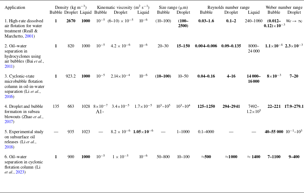

 We=61.4
 Oh=0.026
 Δx=a/50
 Δx=a/60

 We=200
 Oh=1.11
 Re=12.74
 We=200
 Oh=0.006
 Re=2357
 We=35
 Oh=0.006
 Re=986
 We=13
 Oh=0.006
 Re=600
 V0t/(2a)
 −0.5
 0.5

 (We,Δ)
 Oh=0.006
 We=13
 Re=600
 Δ=1
 We=70
 Re=1394
 Δ=0.5
 We=70
 Re=1394
 Δ=1
 We=200
 Re=2357
 Δ=1

 We=13
 Oh=0.006
 Re=600
 Δ=1
 V0

 We=70
 Oh=0.006
 Re=1394
 Δ=0.5
 V0

 We=70
 Oh=0.006
 Re=1394
 Δ=1
 V0

 We=200
 Oh=0.006
 Re=2357
 Δ=1
 V0

 λ=0.5
 λ=2
 (πνlλ2/a2)t
 λ
 V/V0
 λ≈1.19
 We
 Oh
 Δ
 Δ

 We=200
 Oh=0.006
 Re=2357
 Δ=1
 Sd
 Sb
 Kjet
 Ksl
 Kd
 Ev
 Kb
 Γ1
 ×
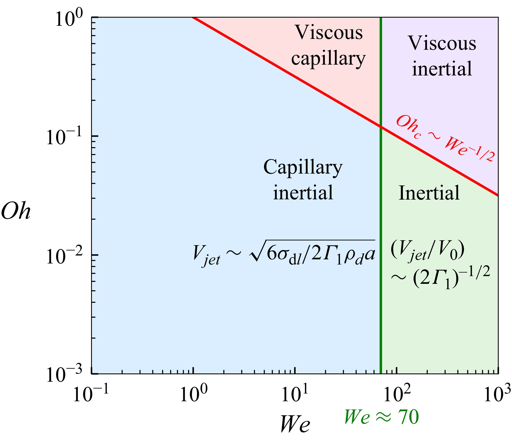
 (We,Oh)
 We≃70
 Ohc∼We−1/2
 Vjet∼6σdl/(2Γ1ρda)
 Vjet/V0∼(2Γ1)−1/2
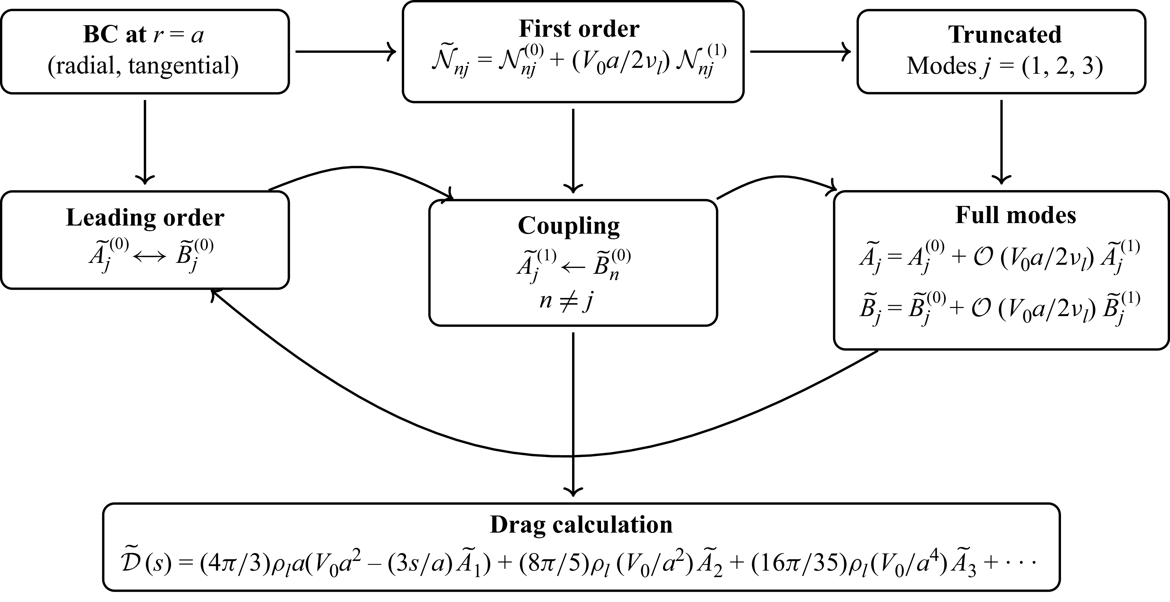


 Open access

