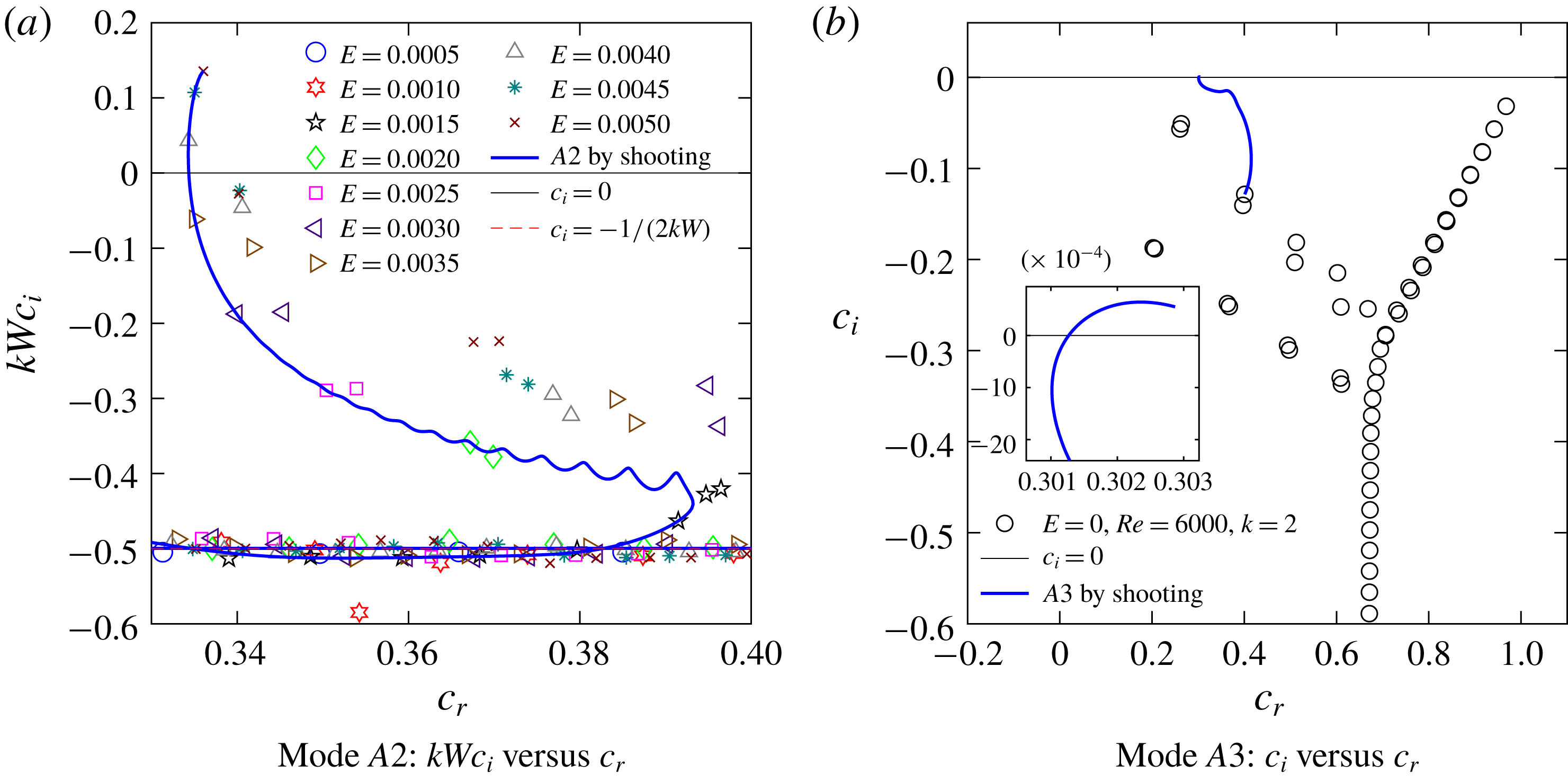
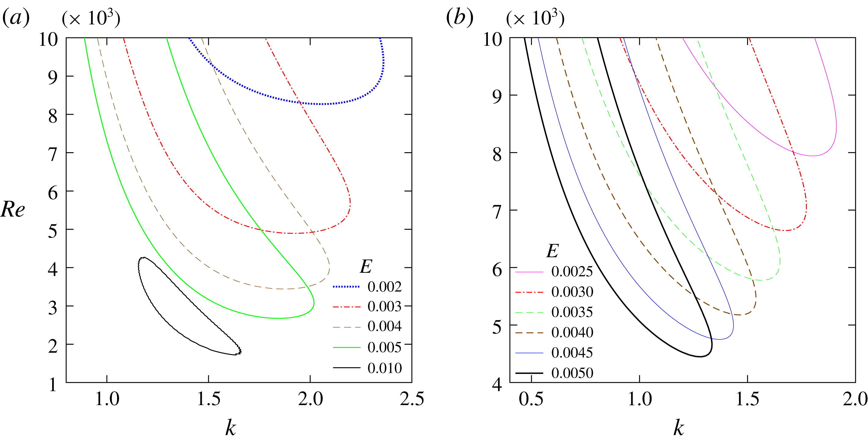
1 Introduction
Plane Poiseuille flow of a Newtonian fluid is predicted to become linearly unstable at a Reynolds number
 $Re\simeq 5772$
, and this instability is often referred to as the ‘Tollmien–Schlichting (TS)’ instability (Schmid & Henningson Reference Schmid and Henningson2001; Drazin Reference Drazin2002). Pressure-driven flows of Newtonian fluids in rectangular channels become unstable in experiments at
 $Re\sim 1000$
(Patel & Head Reference Patel and Head1969; Carlson, Windall & Peters Reference Carlson, Windall and Peters1982; Nishioka & Asai Reference Nishioka and Asai1985). In contrast, the recent experimental study of Srinivas & Kumaran (Reference Srinivas and Kumaran2017) has shown that the flow of dilute polymer solutions in a similar geometry can become unstable at much lower
 $Re\sim 100{-}300$
. Poole (Reference Poole2016) carried out experiments with highly concentrated polymer solutions in rectangular channels with transition occurring at
 $Re\sim 50$
(
 $Re$
being defined based on the viscosity at the wall shear rate), and the instability was proposed as being a consequence of both elasticity and shear thinning. It is well understood, both from experimental and theoretical standpoints, that addition of polymers can lead to novel elastic instabilities in flows with curved streamlines (Shaqfeh Reference Shaqfeh1996) even in the absence of fluid inertia. On the other hand, rectilinear shear flows of (non-shear-thinning) viscoelastic fluids such as plane Couette and Poiseuille flows are presently believed to be linearly stable in the absence of inertia (Ho & Denn Reference Ho and Denn1977; Lee & Finlayson Reference Lee and Finlayson1986; Renardy & Renardy Reference Renardy and Renardy1986), although a rigorous demonstration exists only for plane Couette flow (Renardy Reference Renardy1992). Instabilities in these flows, should they exist, must arise due to an interplay between inertial and elastic effects.
The parameter space relevant to viscoelastic fluid stability, even in the minimal consistent descriptions such as the upper-convected Maxwell (UCM) and the Oldroyd-B constitutive models (the UCM model with an added solvent stress) which neglect effects of shear thinning, is larger: there are at least three dimensionless parameters (the Reynolds and Weissenberg numbers
 $Re$
and
 $W$
, and the ratio
 $\unicode[STIX]{x1D6FD}$
of the solvent to polymer solution viscosity) compared to the Newtonian case where
 $Re$
is the only parameter. Thus, the exclusion of novel (linear) instability mechanisms in viscoelastic shear flows is by no means obvious. Indeed, for plane Poiseuille flow, as discussed in more detail below, earlier investigations have revealed unstable modes other than the (elastically modified) TS mode. Despite this, the traditional viewpoint in the literature, for the two other canonical shear flows, namely plane Couette and pipe Poiseuille flows, has been that of linear stability in the entire
 $Re{-}W{-}\unicode[STIX]{x1D6FD}$
space (Meulenbroek et al.
Reference Meulenbroek, Storm, Bertola, Wagner, Bonn and van Saarloos2003, Reference Meulenbroek, Storm, Morozov and van Saarloos2004; Morozov & van Saarloos Reference Morozov and van Saarloos2005, Reference Morozov and van Saarloos2007; Pan et al.
Reference Pan, Morozov, Wagner and Arratia2013). In marked contrast to this widely held view, we recently (Garg et al.
Reference Garg, Chaudhary, Khalid, Shankar and Subramanian2018) discovered a new centre-mode instability in pressure-driven pipe and channel flows of viscoelastic fluids modelled using the Oldroyd-B constitutive equation. This work underscores the many open questions that remain, especially with regard to the role of elasticity and inertia on the stability of plane shear flows. In the present study, therefore, we revisit the canonical problem of temporal stability of plane shearing flow of a viscoelastic fluid (both Couette and Poiseuille flow profiles) with an objective to explore the possibility of instabilities driven by fluid elasticity that are absent in channel flow of a Newtonian fluid.
We use the upper-convected Maxwell model for our study which predicts a shear-rate-independent viscosity. There have been some earlier studies which have examined the role of shear thinning in the stability of (inelastic) power-law fluids (Liu & Liu Reference Liu and Liu2010), but no qualitatively new instabilities owing to the shear-thinning nature alone have been found. A series of papers by Wilson and co-workers (Wilson & Rallison Reference Wilson and Rallison1999; Wilson & Loridan Reference Wilson and Loridan2015; Castillo & Wilson Reference Castillo and Wilson2017) has shown that shear thinning combined with fluid elasticity, as modelled by a White–Metzner (WM) fluid with a power-law dependence for viscosity on the shear rate, can lead to new instabilities even in the creeping-flow limit. However, in the present work, we focus exclusively on the interplay between elasticity, arising from a microstructure that deforms affinely at a finite rate (that is, the UCM as opposed to the WM model), and inertia; effects of shear thinning are ignored. In the remainder of this Introduction, we provide a brief review of the relevant literature on this subject and motivate the context for the present study.
For parallel shear flows of Newtonian fluids in pipes and channels, temporal linear stability analysis fails to describe the experimentally observed transition (Schmid & Henningson Reference Schmid and Henningson2001): for channels, the theoretical critical Reynolds number
 $Re_{c}=5772$
is much higher than the experimental transition
 $Re\sim 1000$
, as already indicated above; for the pipe geometry, the flow is linearly stable at all
 $Re$
, but experimentally the transition is well known to occur at
 $Re\sim 2000$
. A detailed understanding of transition in the Newtonian case, despite its early origins in the experiments of Reynolds for pipe flow, has only been possible with the recent development of a dynamical systems perspective (Eckhardt et al.
Reference Eckhardt, Schneider, Hof and Westerweel2007; Hof et al.
Reference Hof, de Lozar, Kuik and Westerweel2008, Reference Hof, de Lozar, Avila, Tu and Schneider2010; Avila et al.
Reference Avila, Moxey, Lozar, Barkley and Hof2011; Mullin Reference Mullin2011). The discovery of three-dimensional exact travelling-wave solutions to the Navier–Stokes equations, termed ‘exact coherent states’ (ECS), in the last two decades, has provided the basis for a nonlinear (subcritical) route to transition (Waleffe Reference Waleffe2001; Eckhardt et al.
Reference Eckhardt, Schneider, Hof and Westerweel2007). These solutions bear close resemblance to ‘puffs’ observed in transition experiments (Mullin Reference Mullin2011). The ECS solutions have also been shown to play an important role in the description of structures in the buffer region of turbulent boundary layers, such as streamwise streaks and counter-rotating (streamwise) vortices (Robinson Reference Robinson1991; Jeong et al.
Reference Jeong, Hussain, Schoppa and Kim1997; Waleffe Reference Waleffe2001). It is now believed that, close to transition, turbulence could be interpreted as a phase-space trajectory sampling, in an unpredictable (chaotic) manner, multiple saddle points corresponding to the aforementioned ECS solutions (Budanur et al.
Reference Budanur, Short, Farazmand, Willis and Cvitanović2017).
Experiments have shown that addition of small amounts of polymers to turbulent pipe flow of a Newtonian fluid can significantly reduce the pressure drop (Metzner & Park Reference Metzner and Park1964; Seyer & Metzner Reference Seyer and Metzner1969; Virk Reference Virk1975; White & Mungal Reference White and Mungal2008; Samanta et al.
Reference Samanta, Dubief, Holzner, Schäfer, Morozov, Wagner and Hof2013). While turbulent drag reduction has been achieved in numerical simulations (Sureshkumar, Beris & Handler Reference Sureshkumar, Beris and Handler1997; Dubief et al.
Reference Dubief, White, Terrapon, Shaqfeh, Moin and Lele2004, Reference Dubief, Terrapon, White, Shaqfeh, Moin and Lele2005), an important line of work (Stone, Waleffe & Graham Reference Stone, Waleffe and Graham2002; Stone & Graham Reference Stone and Graham2003; Stone et al.
Reference Stone, Roy, Larson, Waleffe and Graham2004) has analysed the onset of drag reduction in terms of the effect of viscoelasticity on the Newtonian ECS solutions. It has been shown that polymers suppress the Newtonian coherent structures, and that the minimum
 $Re$
for appearance of the ECS solutions increases with increasing
 $E$
, appearing to diverge beyond a critical threshold. This explanation of drag reduction, based on the elastically modified ECS solutions, implicitly assumes that the flow of polymer solutions is linearly stable over the ranges of
 $Re$
and
 $W$
relevant to drag reduction.
Relatively less attention has been devoted to the understanding of turbulence onset in viscoelastic shearing flows. Recent experiments of Samanta et al. (Reference Samanta, Dubief, Holzner, Schäfer, Morozov, Wagner and Hof2013), Chandra, Shankar & Das (Reference Chandra, Shankar and Das2018) and Choueiri, Lopez & Hof (Reference Choueiri, Lopez and Hof2018) on the onset of turbulence in the flow of polyacrylamide solutions in pipes have, however, shown that transition can occur at Reynolds numbers much lower (
 ${\sim}800$
) than the transition Reynolds number for Newtonian fluids in pipes (
 ${\sim}2000$
). At sufficiently high concentrations of the polymer (
 ${>}300~\text{ppm}$
), a new instability is found (Samanta et al.
Reference Samanta, Dubief, Holzner, Schäfer, Morozov, Wagner and Hof2013) for which the onset of transition is independent of the perturbation magnitude and the transition Reynolds numbers can be lower than typical Newtonian values. The ensuing nonlinear flow state is dubbed ‘elasto-inertial turbulence’ to indicate the importance of both fluid elasticity and inertia in this state. Sid, Terrapon & Dubief (Reference Sid, Terrapon and Dubief2018) carried out direct numerical simulations of viscoelastic plane channel flow (using the FENE-P model for the fluid) and demonstrated that the elasto-inertial turbulent state is markedly two-dimensional, further reinforcing the conclusion that the turbulent state that emerges after transition is qualitatively different when compared to its Newtonian counterpart. A recent study by Shekar et al. (Reference Shekar, McMullen, Wang, McKeon and Graham2019) used direct numerical simulations (DNS) to analyse transitional and turbulent channel flows of dilute polymer solutions using the FENE-P model, in a parametric regime where the flow is linearly stable, and where the exact coherent states are suppressed by viscoelasticity. The authors propose a non-normal growth leading to a two-dimensional nonlinear elasto-inertial state wherein the streamwise component of the polymer stress fluctuations is strongly localized at the critical layer closely associated with the original linear eigenmode (an elastically modified TS mode). These results appear to reinforce the earlier conclusion (Sid et al.
Reference Sid, Terrapon and Dubief2018) regarding the two-dimensional nature of the elasto-inertial turbulent state. Our recent theoretical study (Garg et al.
Reference Garg, Chaudhary, Khalid, Shankar and Subramanian2018) also points to the existence of a two-dimensional linear instability in plane channel flows of Oldroyd-B fluids. Clearly, the prevailing theoretical approach towards explaining drag reduction Stone et al. (Reference Stone, Waleffe and Graham2002), Stone & Graham (Reference Stone and Graham2003), Stone et al. (Reference Stone, Roy, Larson, Waleffe and Graham2004), Roy et al. (Reference Roy, Morozov, van Saarloos and Larson2006) using the modified Newtonian ECS solutions, therefore, may not provide a complete description of transition over significant regions of the
 $Re{-}W$
plane. More work is evidently needed with regard to the linear stability of viscoelastic shear flows.
Thus, recent experiments on instabilities in polymer solutions, in both pipes and channels (Samanta et al. Reference Samanta, Dubief, Holzner, Schäfer, Morozov, Wagner and Hof2013; Poole Reference Poole2016; Srinivas & Kumaran Reference Srinivas and Kumaran2017; Wen et al. Reference Wen, Poole, Willis and Dennis2017), direct numerical simulations (Dubief, Terrapon & Soria Reference Dubief, Terrapon and Soria2013; Sid et al. Reference Sid, Terrapon and Dubief2018; Shekar et al. Reference Shekar, McMullen, Wang, McKeon and Graham2019) and linear stability analyses (Garg et al. Reference Garg, Chaudhary, Khalid, Shankar and Subramanian2018) have pointed to the presence of novel instabilities in viscoelastic flows which are absent in Newtonian fluids, and may play a crucial role in transition. In light of these recent efforts, and the dichotomy between them and the prevailing theoretical scenario, the present study explores the possibility of novel instability mechanisms in viscoelastic (plane) channel flows.
2 Survey of earlier stability analyses
In what follows, we specifically review earlier efforts that examine the linear (modal) stability of viscoelastic plane shear flows, and then offer a brief summary of recent efforts on both nonlinear and non-modal stability. Gorodtsov & Leonov (Reference Gorodtsov and Leonov1967) first analysed viscoelastic plane Couette flow based on the UCM model. For
 $Re=0$
, the authors found a pair of stable modes (now known as the zero-Reynolds–Gorodtsov–Leonov (ZRGL) modes). A new class of modes, analogous to shear waves in an elastic solid and propagating at a speed of
 $O(\sqrt{G/\unicode[STIX]{x1D70C}})$
with
 $G=\unicode[STIX]{x1D702}/\unicode[STIX]{x1D706}$
(
 $G$
being the shear modulus and
 $\unicode[STIX]{x1D706}$
being the microstructural relaxation time in the UCM model), but damped on account of the finite relaxation time, emerged for small but finite
 $Re$
(the high-frequency Gorodtsov–Leonov (HFGL) modes). While Gorodtsov & Leonov (Reference Gorodtsov and Leonov1967) inferred an instability due to the HFGL modes in the limit
 $kW\gg 1$
, this was later shown to be incorrect by Renardy & Renardy (Reference Renardy and Renardy1986). Lee & Finlayson (Reference Lee and Finlayson1986) used a shooting method to analyse the stability of both plane Couette and Poiseuille flows and focussed on the regime
 $k\gg 1$
, with
 $Re,W\sim O(1)$
. The authors found only stable eigenmodes for both flows, but the shooting method used accessed only a small subset of the full eigenspectrum. Renardy & Renardy (Reference Renardy and Renardy1986) used a spectral method which clarified the nature of the complete eigenspectrum and showed that plane Couette flow of an UCM fluid is indeed stable at finite
 $Re$
and
 $W$
. Kumar & Shankar (Reference Kumar and Shankar2005) used a singular perturbation analysis and showed that the finite,
 $Re$
discrete, spectrum reported by Renardy & Renardy (Reference Renardy and Renardy1986) was, in fact, a continuation to finite
 $Re$
of the ZRGL and HFGL modes originally found by Gorodtsov & Leonov (Reference Gorodtsov and Leonov1967) for
 $Re\ll 1$
. In summary, the discrete spectrum for plane Couette flow, based on the UCM model, consists of the ZRGL and HFGL modes for any finite
 $Re$
, and an additional continuous spectrum consisting of singular modes all of which relax at a rate
 $\unicode[STIX]{x1D706}$
, with phase speeds in the base-state range of velocities. All of the aforementioned investigations, and other more recent ones (Chokshi & Kumaran Reference Chokshi and Kumaran2009), have confirmed that plane Couette flow of a UCM fluid is stable in the
 $Re{-}W$
plane, a conclusion reinforced by our results reported in § 4.
Porteous & Denn (Reference Porteous and Denn1972) studied the role of elasticity on the TS instability in viscoelastic plane Poiseuille flow by using a UCM model, and showed that at high Reynolds numbers there were three unstable eigenmodes (these modes are labelled as
 $A1(a)$
,
 $A1(b)$
and
 $A2$
in the present work), of which the authors explored
 $A1(a)$
in detail, and demonstrated that an increase in the elasticity number
 $E$
destabilized this mode; as elaborated later in § 4.2, the mode
 $A1(a)$
arises from the original (Newtonian) TS mode. On the other hand, at low Reynolds number (Ho & Denn Reference Ho and Denn1977), plane Poiseuille flow was found to be stable. Lee & Finlayson (Reference Lee and Finlayson1986) explored both symmetric and antisymmetric modes for plane Poiseuille flow of a UCM fluid using a shooting method for wide ranges of
 $k$
and
 $W$
with
 $Re=1$
, finding only stable modes. Sureshkumar & Beris (Reference Sureshkumar and Beris1995b
) used an Arnoldi algorithm to obtain the first few unstable eigenvalues for plane Poiseuille flow of UCM and Oldroyd-B fluids, the latter involving the additional parameter
 $\unicode[STIX]{x1D6FD}$
, defined as the ratio of viscosity of the solvent to that of the polymer solution;
 $\unicode[STIX]{x1D6FD}=0$
represents a UCM fluid and
 $\unicode[STIX]{x1D6FD}=1$
represents a Newtonian fluid. For the UCM fluid, the authors discussed unstable modes belonging to two eigenfamilies (labelled in this work as
 $A1(a)$
and
 $A1(b)$
). They showed that, for the mode
 $A1(a)$
, to begin with, an increase in
 $E$
leads to a reduction in the critical
 $Re$
compared to a Newtonian fluid, but with further increase in
 $E$
, the critical
 $Re$
increases again, suggesting that elasticity has a non-monotonic effect on flow stability; this initial decrease is consistent with the findings of Porteous & Denn (Reference Porteous and Denn1972) above. This behaviour was further analysed by Sadanandan & Sureshkumar (Reference Sadanandan and Sureshkumar2002) based on an analysis of the perturbation kinetic energy and vorticity. The unstable modes in the UCM case were strongly stabilized for non-zero
 $\unicode[STIX]{x1D6FD}$
in an Oldroyd-B fluid. (Sureshkumar & Beris Reference Sureshkumar and Beris1995b
; Sadanandan & Sureshkumar Reference Sadanandan and Sureshkumar2002). As mentioned earlier, we recently found a new type of instability in viscoelastic channel and pipe flows of an Oldroyd-B fluid (Garg et al.
Reference Garg, Chaudhary, Khalid, Shankar and Subramanian2018), absent both in the Newtonian and UCM limits, with profound implications for the transition scenario in viscoelastic shearing flows.
While the above discussion was focussed on quasi-linear constitutive relations, there has been some work on flow stability using nonlinear and non-local constitutive models. Grillet et al. (Reference Grillet, Bogaerds, Peters and Baaijens2002) in their numerical study, in the creeping-flow limit, of the nonlinear Phan-Thien–Tanner (PTT) and Giesekus models found plane Couette flow to be unstable in the former case. To our knowledge, this is the only reported instability of plane Couette flow using a local (but nonlinear) viscoelastic constitutive relation. However, plane Poiseuille flow was found to be unstable in both PTT and Giesekus models. Grillet et al. (Reference Grillet, Bogaerds, Peters and Baaijens2002) also proposed mechanisms for instabilities in both flows based on the coupling between base-state stresses and the gradients of perturbation velocities. They demonstrated the similarity in driving mechanisms of instability for Poiseuille flow in both the PTT and Giesekus models. In Poiseuille flow, a perturbation near the wall disrupts the stratification of the normal stresses near the wall reinforcing the initial perturbation which in turn triggers the instability. For Couette flow, the differences in the shear rates arising from shear thinning are reinforced by the initial velocity perturbations, thereby leading to an instability. Chokshi & Kumaran (Reference Chokshi and Kumaran2009) investigated the stability of plane Couette flow for a non-local Oldroyd-B model with a coupling between the stress and polymer concentration, the latter being governed by an additional convection–diffusion equation. This non-local model was found to exhibit an instability beyond a threshold
 $W$
. The authors argued that the otherwise stable diffusive modes are destabilized by stress-induced migration of the polymer, suggesting that the growth/decay rates of these modes will be determined by the polymer diffusion time scale. This time scale is, however, expected to be exceedingly long when the solution is away from its critical point. Cromer et al. (Reference Cromer, Villet, Fredrickson and Leal2013), Cromer, Fredrickson & Leal (Reference Cromer, Fredrickson and Leal2014) have recently used a Rolie–Poly model, again with a coupling of polymer stress to concentration, and noted a linear instability of plane Couette flow beyond a critical
 $W$
; nonlinear simulations showed that this instability resulted in a banded velocity profile.
The vast majority of investigations based on quasi-linear constitutive models not having found a linear instability for inertia-less viscoelastic shear flows motivated a series of studies by van Saarloos and co-workers (Bertola et al.
Reference Bertola, Meulenbroek, Wagner, Storm, Morozov, van Saarloos and Bonn2003; Meulenbroek et al.
Reference Meulenbroek, Storm, Bertola, Wagner, Bonn and van Saarloos2003, Reference Meulenbroek, Storm, Morozov and van Saarloos2004; Morozov & van Saarloos Reference Morozov and van Saarloos2005, Reference Morozov and van Saarloos2007) examining the role of nonlinear mechanisms in canonical rectilinear shearing flows (plane Couette, plane Poiseuille and pipe Poiseuille) of a UCM fluid. Another motivation underlying these studies was an explanation of the melt fracture phenomenon (Bertola et al.
Reference Bertola, Meulenbroek, Wagner, Storm, Morozov, van Saarloos and Bonn2003), a common instability encountered in polymer extrusion processes. These studies have identified a nonlinear subcritical instability in these flows that becomes operative via a saddle-node bifurcation at a critical
 $W\sim O(1)$
. Further, the magnitude of the perturbation required to trigger instability decreases with increasing
 $W$
. All these studies were restricted to the creeping-flow limit, with the weakly nonlinear stability analysis being based on the ZRGL mode (Gorodtsov & Leonov Reference Gorodtsov and Leonov1967). However, within the linear stability framework, the continuation of the ZRGL mode to finite
 $Re$
leads to it no longer being the least stable mode, making the weakly nonlinear analysis about the GL mode suspect at higher
 $Re$
. Therefore, more work is needed to clarify the relevance of the weakly nonlinear stability of viscoelastic flows at higher
 $Re$
.
With the Oldroyd-B model exhibiting only stable modes in plane Couette flow, there have been many (linear) non-modal analyses to understand the transient growth of disturbances in viscoelastic flows, both in the creeping-flow limit and in presence of inertia (Doering, Eckhardt & Schumacher Reference Doering, Eckhardt and Schumacher2006; Hoda, Jovanovic & Kumar Reference Hoda, Jovanovic and Kumar2008, Reference Hoda, Jovanovic and Kumar2009; Jovanovic & Kumar Reference Jovanovic and Kumar2010, Reference Jovanovic and Kumar2011; Zhang et al.
Reference Zhang, Lashgari, Zaki and Brandt2013; Page & Zaki Reference Page and Zaki2014). For Newtonian fluids, it is now well understood that the non-normal nature of the underlying differential operator governing the stability of the flows allows for significant growth of initial conditions before the onset of asymptotic decay at large times. In the absence of a linear modal instability, it has been argued for Newtonian fluids that this (linear) transient growth of infinitesimal perturbations could eventually make the nonlinear terms important, thus making this combination of initial transient growth and subsequent nonlinear evolution a possible explanation for transition in Newtonian fluids (Schmid & Henningson Reference Schmid and Henningson2001). Indeed, the initial conditions that exhibit the maximum transient growth in Newtonian fluids correspond to alternating regions of high and low streamwise velocities (termed ‘streaks’) seen in both experimental observations and numerical simulations of transition in Newtonian fluids, and form a basic element of the ECSs mentioned above. Doering et al. (Reference Doering, Eckhardt and Schumacher2006) first demonstrated that, even at arbitrarily small
 $Re$
, viscoelastic flows could exhibit transient growth at non-zero Weissenberg number
 $W$
, and thence argued that there is no finite
 $Re$
below which the perturbations decay monotonically. Jovanovic & Kumar (Reference Jovanovic and Kumar2010) studied transient growth in plane Couette flow of an Oldroyd-B fluid, and showed that for streamwise invariant three-dimensional disturbances, both velocity and polymer stress fluctuations exhibit significant transient growth even in the absence of inertia. Another class of studies (Hoda et al.
Reference Hoda, Jovanovic and Kumar2008, Reference Hoda, Jovanovic and Kumar2009; Jovanovic & Kumar Reference Jovanovic and Kumar2011; Page & Zaki Reference Page and Zaki2014) focussed on the (linear) response of viscoelastic flows to stochastic forcing in the governing equations. These studies have shown that the most amplified disturbances again have no streamwise variation, but have an
 $O(1)$
spanwise wavenumber, provided that the elasticity of the fluid is sufficiently strong. Zhang et al. (Reference Zhang, Lashgari, Zaki and Brandt2013) carried out both linear modal and non-modal analyses of channel flows of Oldroyd-B and FENE-P fluids when inertial effects are dominant, by considering both streamwise invariant and oblique disturbances. They showed that the ratio of the relaxation time and the time scale over which the instability evolves plays a significant role with regard to the stabilizing or destabilizing nature of the polymer. When this ratio is small, destabilization was observed, while the opposite happens when the ratio becomes large, with maximum amplification happening when the ratio is of order unity.
Thus, nonlinear or non-modal effects are often invoked to understand and explain instabilities in viscoelastic shearing flows. This is despite the absence of a comprehensive search of the
 $Re{-}W{-}\unicode[STIX]{x1D6FD}$
parameter space for new linearly unstable modes which could be primarily driven by elastic effects. As already discussed, both earlier and recent experimental efforts in pipes and channels (Samanta et al.
Reference Samanta, Dubief, Holzner, Schäfer, Morozov, Wagner and Hof2013; Poole Reference Poole2016; Srinivas & Kumaran Reference Srinivas and Kumaran2017; Wen et al.
Reference Wen, Poole, Willis and Dennis2017) are suggestive of linear instability mechanisms operative in these geometries. This belief has been reinforced in a recent study (Garg et al.
Reference Garg, Chaudhary, Khalid, Shankar and Subramanian2018) which has shown both pipe and plane Poiseuille flows of viscoelastic Oldroyd-B fluids are linearly unstable, with the predicted transition
 $Re$
being in qualitative agreement with experimental results for the flow of polymer solutions in pipes. The unstable modes analysed in the said study belong to a class of ‘centre modes’ with phase speeds close to the maximum velocity of the base flow, and with disturbances increasingly confined near the pipe or channel centreline, as
 $Re$
is increased. This is in marked contrast to the TS instability of Newtonian plane channel flow, where the unstable mode can be termed as a ‘wall mode’ with disturbances being localized close to the solid boundary.
The question that arises naturally, then, is whether there are qualitatively new unstable wall modes in viscoelastic channel flows that are absent in a Newtonian fluid. This is the focus of the present study. For the sake of comparison (and contrast) we also report results for viscoelastic plane Couette flow. We build on and augment the earlier work on temporal stability of viscoelastic channel flows (Porteous & Denn Reference Porteous and Denn1972; Ho & Denn Reference Ho and Denn1977; Lee & Finlayson Reference Lee and Finlayson1986; Sureshkumar & Beris Reference Sureshkumar and Beris1995b
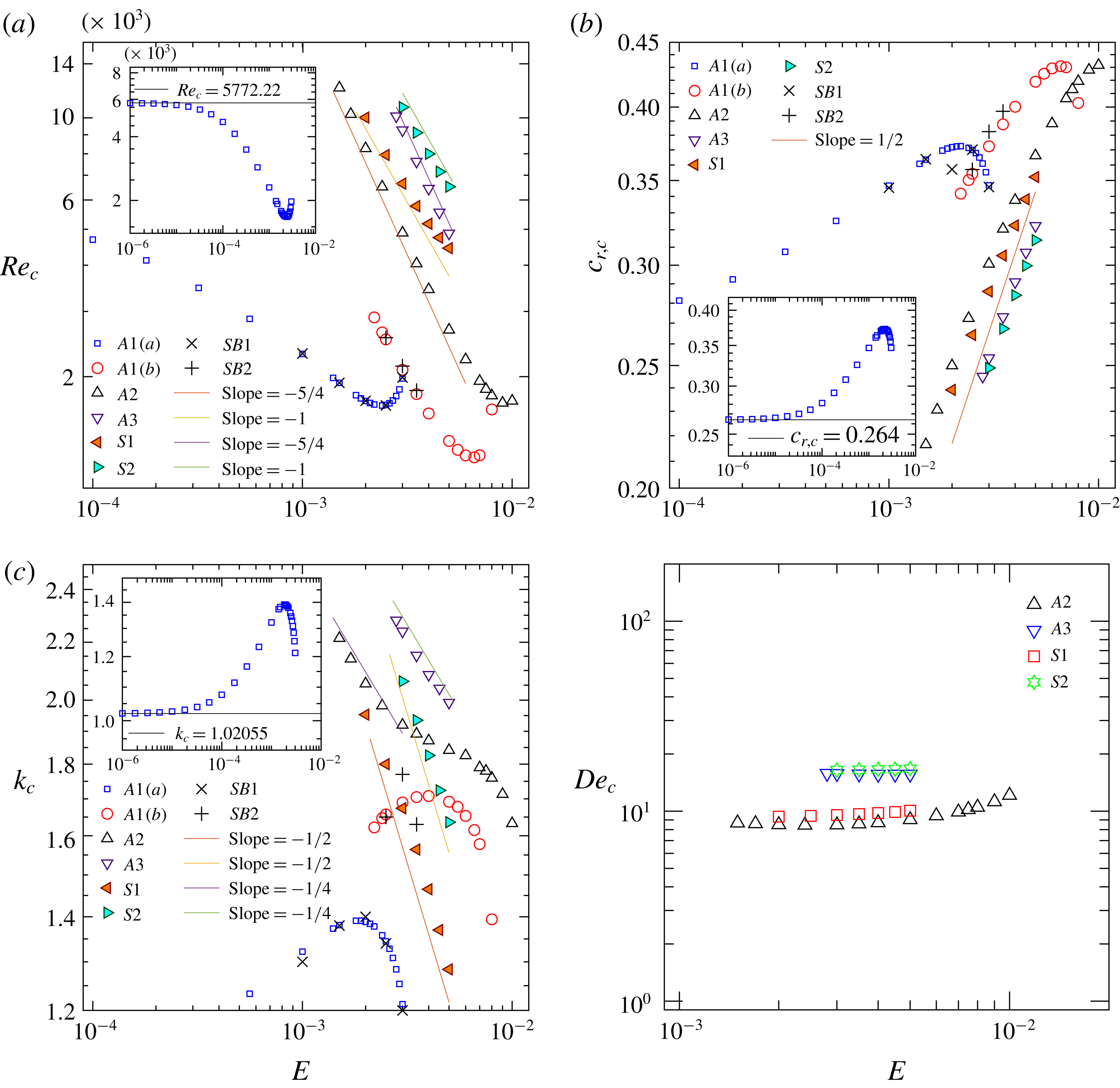
) by expanding the parameter space of our search for unstable eigenmodes for a UCM fluid. We show that there are multiple new unstable modes (suggestive of an infinite elasto-inertial hierarchy) in viscoelastic plane Poiseuille flow that are caused by the combined effects of inertia and elasticity of the fluid, and that are therefore absent in the Newtonian limit. We characterize these new unstable modes in terms of their neutral stability curves and examine how the respective critical Reynolds numbers
 $Re_{c}$
change as a function of
 $E$
. Two different numerical schemes, based on a pseudo-spectral and a shooting method, are used to obtain all numerical results reported here.
The remainder of this paper is organized as follows: in § 3, we present a description of the system considered for investigation and the equations governing small-amplitude perturbations. Our numerical results, presented in § 4, are structured as follows: in § 4.1, we discuss the eigenspectra, eigenfunctions and their salient features to illustrate the general structure of the elasto-inertial eigenspectrum for both plane Couette and Poiseuille flows, and to distinguish between the various unstable eigenmodes. The eigenmodes are classified into three major classes: the continuous spectrum balloon (§ 4.1.1), the HFGL modes (§ 4.1.2) and modes belonging to an ‘hourglass’ structure (§ 4.1.4). Section 4.1.3 presents a WKBJ (Wentzel–Kramers–Brillouin–Jeffreys) based asymptotic analysis of the HFGL modes in the limit
 $Re\gg 1$
,
 $(ReW)^{-1/2}\ll 1$
. The evolution of the eigenspectrum with increasing elasticity of the fluid is discussed in § 4.1.5. The discussion in § 4.2, on the instabilities predicted for plane Poiseuille flow, first focusses on the effect of elasticity on the Newtonian TS instability, and the new features found in this study in terms of coalescence/bifurcation of the continuation of the TS mode with a new elasto-inertial mode as well as the disappearance of the instability at sufficiently high
 $E$
(§ 4.2.1). Section 4.2.2 discusses the new elasto-inertial instabilities found in plane Poiseuille flow in terms of the eigenspectra and eigenfunctions, along with neutral stability curves in the
 $Re{-}k$
-plane. The origin of the new elasto-inertial modes in the Newtonian limit, of
 $E\rightarrow 0$
, is discussed in § 4.2.3. Section 4.2.4 shows the evolution of neutral curves for the new instabilities with increasing elasticity, and the associated scalings for the critical parameters. Finally in § 5, we conclude this paper with a brief summary of the key findings. Validation of the numerical schemes employed is briefly discussed in §§ A.1 and A.2.
3 Problem formulation and numerical method
3.1 Governing equations
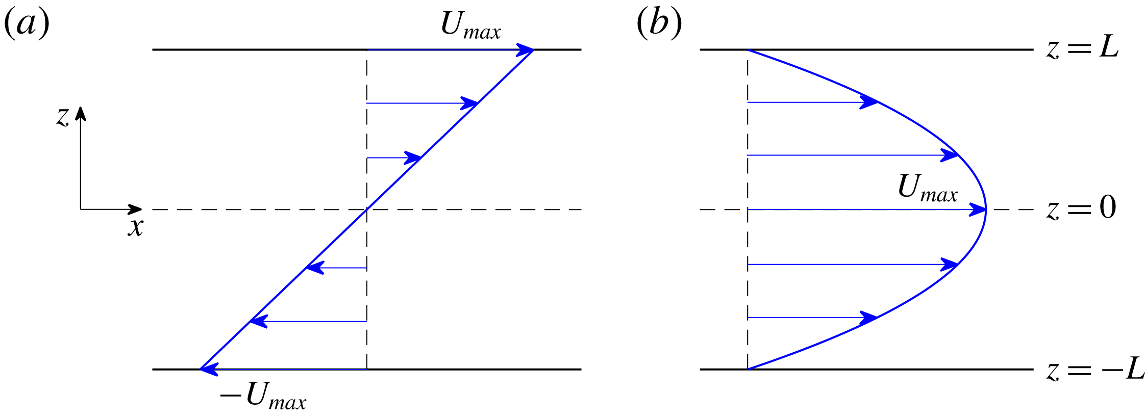
The stability problem considered is that of a viscoelastic shearing flow between a pair of plates separated by a distance
 $2L$
, as shown in figure 1. The unidirectional base flow is along the
 $x$
-axis and the direction normal to the plates is taken along the
 $z$
-axis. The viscoelastic fluid is modelled using the upper-convected Maxwell model with a density
 $\unicode[STIX]{x1D70C}$
, viscosity
 $\unicode[STIX]{x1D702}$
and a (microstructural) relaxation time
 $\unicode[STIX]{x1D706}$
. In the case of plane Poiseuille flow, both the plates are fixed and a pressure gradient along the
 $x$
-axis drives the flow. For plane Couette flow, the top and bottom plates move in opposite directions with a velocity of magnitude
 $U_{max}$
.
Schematic diagram showing the planar flow geometries: (a) Couette flow; (b) Poiseuille flow and dimensional coordinate systems considered.

The following scales are used for non-dimensionalizing the governing equations: the channel half-width
 $L$
for lengths, the base-flow maximum speed
 $U_{max}$
for velocities,
 $L/U_{max}$
for time and
 $\unicode[STIX]{x1D702}U_{max}/L$
for the pressure and stresses. The governing (non-dimensional) continuity and Cauchy momentum equations are given by
 $$\begin{eqnarray}\displaystyle \unicode[STIX]{x1D735}\boldsymbol{\cdot }\boldsymbol{v}=0,\quad Re\left(\frac{\unicode[STIX]{x2202}\boldsymbol{v}}{\unicode[STIX]{x2202}t}+(\boldsymbol{v}\boldsymbol{\cdot }\unicode[STIX]{x1D735})\boldsymbol{v}\right)=-\unicode[STIX]{x1D735}p+\unicode[STIX]{x1D735}\boldsymbol{\cdot }\unicode[STIX]{x1D64F}. & & \displaystyle\end{eqnarray}$$
Here,
 $\boldsymbol{v}$
is the velocity field,
 $p$
is the pressure and
 $\unicode[STIX]{x1D64F}$
is the polymeric stress tensor in the fluid. The polymeric stress tensor is assumed to be given by the UCM constitutive relation (Larson Reference Larson1988) as
 $$\begin{eqnarray}\displaystyle W\left({\displaystyle \frac{\unicode[STIX]{x2202}\unicode[STIX]{x1D64F}}{\unicode[STIX]{x2202}t}}+(\boldsymbol{v}\boldsymbol{\cdot }\unicode[STIX]{x1D735})\unicode[STIX]{x1D64F}-(\unicode[STIX]{x1D735}\boldsymbol{v})^{\text{T}}\boldsymbol{\cdot }\unicode[STIX]{x1D64F}-\unicode[STIX]{x1D64F}\boldsymbol{\cdot }(\unicode[STIX]{x1D735}\boldsymbol{v})\right)+\unicode[STIX]{x1D64F}=(\unicode[STIX]{x1D735}\boldsymbol{v}+\unicode[STIX]{x1D735}\boldsymbol{v}^{\text{T}}). & & \displaystyle\end{eqnarray}$$
The dimensionless groups relevant to the system are the Reynolds number
 $Re=\unicode[STIX]{x1D70C}U_{max}L/\unicode[STIX]{x1D702}$
and the Weissenberg number
 $W=\unicode[STIX]{x1D706}U_{max}/L$
. The Reynolds number measures the ratio of inertial to viscous stresses in the flow, while the Weissenberg number, defined as the ratio of the relaxation time of the fluid to the flow time scale, measures the relative importance of elastic to viscous forces (Poole Reference Poole2012). We also use the elasticity number
 $E=W/Re=\unicode[STIX]{x1D706}\unicode[STIX]{x1D702}/(\unicode[STIX]{x1D70C}L^{2})$
in the following discussion to characterize the stability of the system (Graham Reference Graham2014; Garg et al.
Reference Garg, Chaudhary, Khalid, Shankar and Subramanian2018). The elasticity number is fixed for a given choice of channel and polymer solution, and hence is useful when making comparisons with experiments. The boundary conditions for the velocity field are the no-slip conditions at the two plates
 $z=\pm 1$
.
As the upper-convected nonlinear terms do not affect the determination of the uni-directional velocity profile, the base-state velocity profiles, for the UCM model considered, are the same as the corresponding Newtonian ones,
 $$\begin{eqnarray}\displaystyle \overline{\boldsymbol{v}}=\left[\begin{array}{@{}c@{}}U(z)\\ 0\\ 0\end{array}\right], & & \displaystyle\end{eqnarray}$$
where
 $U(z)=1-z^{2}$
for plane Poiseuille flow and
 $U(z)=z$
for plane Couette flow. The base-state stress tensor, however, is affected by the upper-convected terms, and is given by
 $$\begin{eqnarray}\displaystyle \overline{\unicode[STIX]{x1D64F}}=\left[\begin{array}{@{}ccc@{}}2W(U^{\prime })^{2} & 0 & U^{\prime }\\ 0 & 0 & 0\\ U^{\prime } & 0 & 0\end{array}\right], & & \displaystyle\end{eqnarray}$$
where
 $U^{\prime }\equiv \text{d}U/\text{d}z$
. Thus, relative to the Newtonian case, there exists an additional tension along the base-state streamlines proportional to the square of the velocity gradient.
3.2 Linear stability analysis
A classical linear temporal stability analysis is carried out for this system, wherein infinitesimal perturbations are imposed on the base-state physical quantities. The analysis carried out in this study is restricted to two-dimensional (in the
 $x$
–
 $z$
plane) perturbations with variations in the (spanwise)
 $y$
-direction neglected. Similar to the Newtonian case (Drazin Reference Drazin2002), Squire’s theorem, which shows that two-dimensional disturbances are the most unstable ones, is applicable (Bistagnino et al.
Reference Bistagnino, Boffetta, Celani, Mazzino, Puliafito and Vergassola2007). Three-dimensional perturbations could well be important in an analysis of transient growth (Zhang et al.
Reference Zhang, Lashgari, Zaki and Brandt2013), but consideration of two-dimensional perturbations is sufficient within the framework of a modal analysis. The velocity and stress fields, after imposition of disturbances, become
 $$\begin{eqnarray}\displaystyle \boldsymbol{v} & = & \displaystyle \overline{\boldsymbol{v}}+\hat{\boldsymbol{v}},\end{eqnarray}$$
 $$\begin{eqnarray}\displaystyle p & = & \displaystyle \overline{p}+\hat{p},\end{eqnarray}$$
 $$\begin{eqnarray}\displaystyle \unicode[STIX]{x1D64F} & = & \displaystyle \overline{\unicode[STIX]{x1D64F}}+\hat{\unicode[STIX]{x1D64F}},\end{eqnarray}$$
 $$\begin{eqnarray}\displaystyle \hat{\boldsymbol{v}}=\left[\begin{array}{@{}c@{}}\hat{v}_{x}\\ 0\\ \hat{v}_{z}\end{array}\right]\quad \text{and}\quad \hat{\unicode[STIX]{x1D64F}}=\left[\begin{array}{@{}ccc@{}}\hat{\unicode[STIX]{x1D70F}}_{xx} & 0 & \hat{\unicode[STIX]{x1D70F}}_{xz}\\ 0 & 0 & 0\\ \hat{\unicode[STIX]{x1D70F}}_{xz} & 0 & \hat{\unicode[STIX]{x1D70F}}_{zz}\end{array}\right]. & & \displaystyle\end{eqnarray}$$
Here,
 $\hat{f}$
represents a perturbation to the dynamical quantity
 $f$
. The governing (3.1) and (3.2) are then linearized about the base state. The perturbation quantities are expressed in terms of elementary Fourier modes, in the
 $x$
-direction, of the following form:
 $$\begin{eqnarray}\displaystyle \hat{f}(x,z;t)=\tilde{f}(z)\exp \{\text{i}k(x-ct)\}, & & \displaystyle\end{eqnarray}$$
where
 $k$
is the wavenumber along the
 $x$
-axis, and
 $c=c_{r}+\text{i}c_{i}$
is the (complex) wave speed. The flow is temporally unstable (stable) if
 $c_{i}>0$
(
 $c_{i}<0$
). Substituting (3.7) in the linearized versions of (3.1) and (3.2), we obtain the following set of linearized equations governing the eigenvalue
 $c$
:
 $$\begin{eqnarray}\displaystyle & \displaystyle \mathscr{D}\tilde{v}_{z}+\text{i}k\tilde{v}_{x}=0, & \displaystyle\end{eqnarray}$$
 $$\begin{eqnarray}\displaystyle & \displaystyle Re\{\text{i}k(U-c)\tilde{v}_{x}+\tilde{v}_{z}U^{\prime }\}=-\text{i}k\tilde{p}+\text{i}k\tilde{\unicode[STIX]{x1D70F}}_{xx}+\mathscr{D}\tilde{\unicode[STIX]{x1D70F}}_{xz}, & \displaystyle\end{eqnarray}$$
 $$\begin{eqnarray}\displaystyle & \displaystyle Re\text{i}k(U-c)\tilde{v}_{z}=-\mathscr{D}\tilde{p}+\text{i}k\tilde{\unicode[STIX]{x1D70F}}_{xz}+\mathscr{D}\tilde{\unicode[STIX]{x1D70F}}_{zz}, & \displaystyle\end{eqnarray}$$
 $$\begin{eqnarray}\displaystyle & \displaystyle \{1+\text{i}kW(U-c)\}\tilde{\unicode[STIX]{x1D70F}}_{xx}=[\{2WU^{\prime }\mathscr{D}+2\text{i}k+4\text{i}kW^{2}(U^{\prime })^{2}\}\tilde{v}_{x}-4W^{2}U^{\prime }U^{\prime \prime }\tilde{v}_{z}]+2WU^{\prime }\tilde{\unicode[STIX]{x1D70F}}_{xz}, & \displaystyle \nonumber\\ \displaystyle & & \displaystyle\end{eqnarray}$$
 $$\begin{eqnarray}\displaystyle & \displaystyle \{1+\text{i}kW(U-c)\}\tilde{\unicode[STIX]{x1D70F}}_{xz}=[\mathscr{D}\tilde{v}_{x}+\{\text{i}k+2\text{i}kW^{2}(U^{\prime })^{2}-WU^{\prime \prime }\}\tilde{v}_{z}]+WU^{\prime }\tilde{\unicode[STIX]{x1D70F}}_{zz}, & \displaystyle\end{eqnarray}$$
 $$\begin{eqnarray}\displaystyle & \displaystyle \{1+\text{i}kW(U-c)\}\tilde{\unicode[STIX]{x1D70F}}_{zz}=2(\mathscr{D}+\text{i}kWU^{\prime })\tilde{v}_{z}, & \displaystyle\end{eqnarray}$$
where the notation
 $\mathscr{D}f\equiv \text{d}f/\text{d}z$
. The no-slip conditions at the walls are given by
 $$\begin{eqnarray}\displaystyle \tilde{v}_{x}(\pm 1)=0,\quad \tilde{v}_{z}(\pm 1)=0. & & \displaystyle\end{eqnarray}$$
3.3 Numerical method
The linearized governing equations are solved using two different methods. We obtained the eigenspectrum using a pseudo-spectral method based on an expansion of the relevant fields using Chebyshev polynomials. The number of collocation points required to capture physically genuine eigenvalues is varied as required by the particular parameter regime examined. Convergence in this method is achieved (Schmid & Henningson Reference Schmid and Henningson2001) by comparing the eigenspectra for two different values of
 $N$
, and subsequently filtering them subject to a prescribed tolerance, as discussed in appendix A. However, in the eigenspectrum for viscoelastic flows, there is also a continuous spectrum with
 $c_{r}$
taking any value in the base-state range of velocities. The continuous spectrum (as discussed a little later in § 4.1.1) is not accurately captured by the spectral method, and often manifests as a balloon-like structure in the overall eigenspectrum. The spread of this balloon (along the
 $c_{i}$
-axis) is sensitively dependent on
 $N$
, leading to the different appearances of the filtered and the unfiltered spectra.
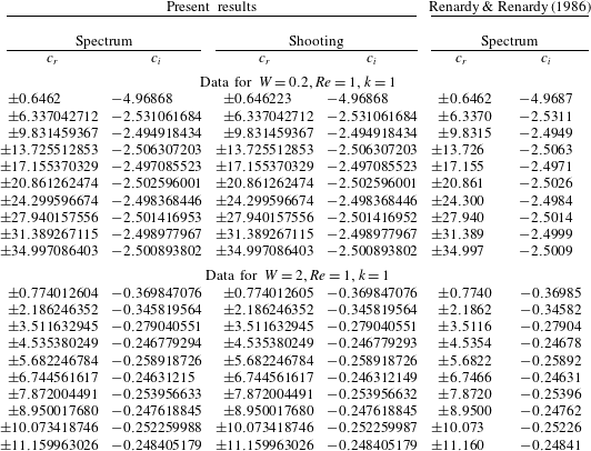
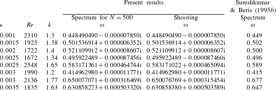
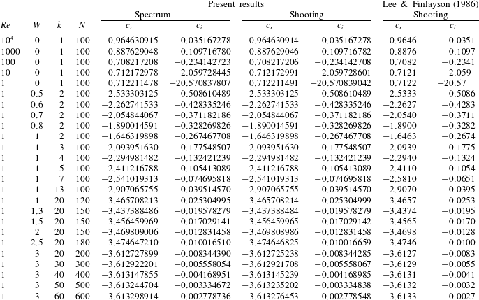
The eigenvalues obtained using the spectral code were further verified using a shooting method with a stiff integrator coupled with Gram–Schmidt orthonormalization during integration. A Newton–Raphson scheme was used to determine the eigenvalue. Both these methods have their own advantages and limitations. Use of the two methods together allows us to exploit the advantages of both. The spectral method provides the entire eigenspectrum without initial guesses. As a result, it is possible to infer the generic features of the eigenspectrum, classify eigenvalues into different groups, etc., as will be discussed below. However, it is well known that spectral methods can yield unphysical and spurious eigenvalues (Schmid & Henningson Reference Schmid and Henningson2001). The shooting method does not have the problem of spurious eigenvalues, but requires a good initial guess for the Newton–Raphson iterative procedure. The question of whether the eigenvalues, obtained from the spectral method are physically genuine, can therefore be confirmed by providing them as initial guesses to the shooting method. A brief description of both methods is given in § A.1. We have validated our numerical schemes by comparing the present results with those available in the literature for plane Couette and plane Poiseuille flows of both Newtonian and UCM fluids. Section A.2 discusses the validation of our numerical procedure.
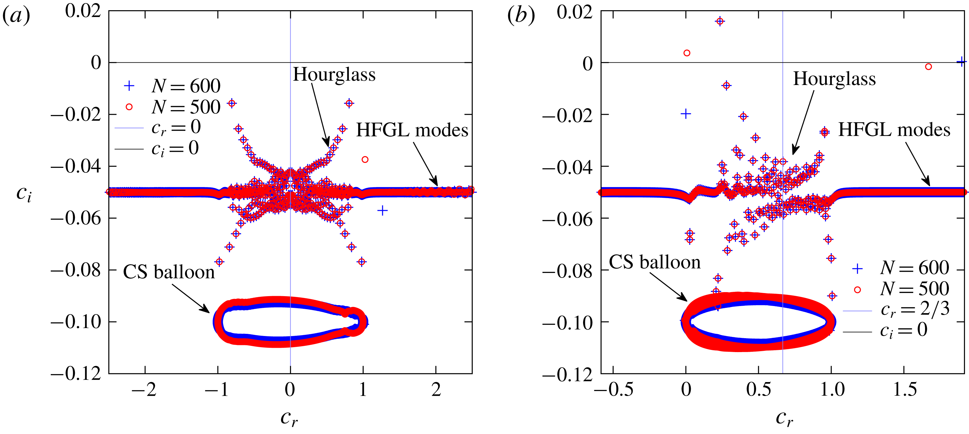
Unfiltered eigenspectra for (a) plane Couette and (b) plane Poiseuille flows for
 $E=0.001,k=1.0,Re=10^{4}$
with
 $N=$
 $500$
and
 $600$
. The distinctive features are labelled within the spectra.

4 Results and discussion
We first discuss the results obtained for both plane Couette and Poiseuille flows of a UCM fluid, focussing on the generic features of the elasto-inertial spectrum. This is followed by the discussion of unstable modes for the plane Poiseuille case. In this work, our search for unstable eigenvalues was limited to
 $Re\leqslant 10^{4}$
and
 $E\leqslant 0.01$
. The restriction in parameter space was necessary due to the larger computational time required for convergence of eigenvalues for
 $Re>10^{4}$
especially for
 $E\sim 0.005$
and higher, as discussed in subsequent sections. For future reference, it is useful to recall that the Newtonian eigenspectrum for plane Poiseuille flow, at sufficiently high
 $Re$
, exhibits a characteristic ‘Y-shaped’ structure (Schmid & Henningson Reference Schmid and Henningson2001). There are thus three distinct (‘APS’) branches of eigenvalues: the ‘
 $A$
-branch’ corresponding to ‘wall modes’ with phase speeds approaching zero, the ‘
 $P$
-branch’ corresponding to ‘centre modes’ with phase speeds tending to the centreline velocity and the ‘
 $S$
-branch’ with modes having phase speeds equal to two thirds of the centreline base-flow velocity. A wall mode belonging to the
 $A$
-branch becomes unstable in plane channel flow of a Newtonian fluid at
 $Re>5772$
. In contrast, on account of the antisymmetry of plane Couette flow, its Newtonian eigenspectrum lacks a
 $P$
-branch. There are two
 $A$
-branches instead, with the modes along these branches having phase speeds tending to those of the respective boundaries.
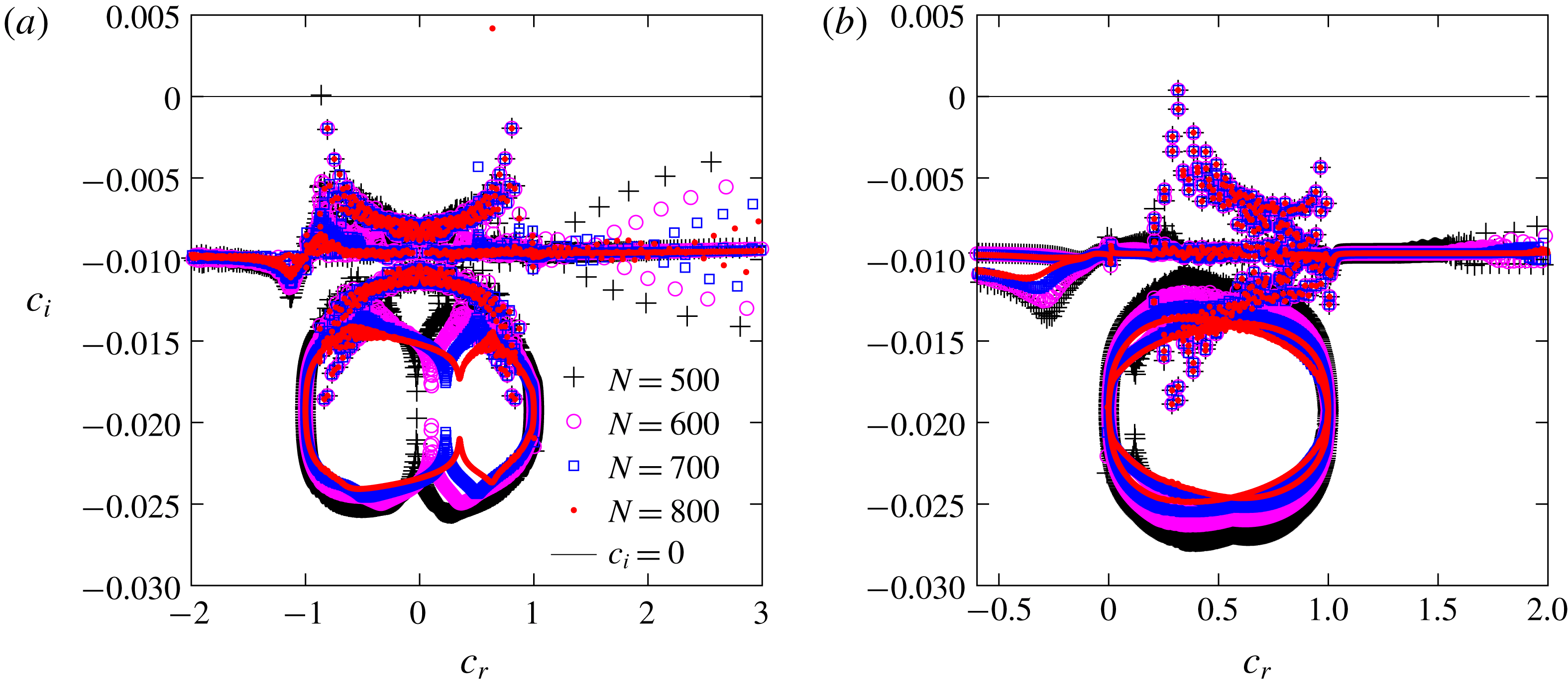
Unfiltered eigenspectra for (a) plane Couette and (b) plane Poiseuille flows for
 $E=0.005,k=2.0,Re=5200$
with
 $N=500$
,
 $600$
,
 $700$
and
 $800$
. In the spectra for plane Couette flow, one spurious unstable mode is present for
 $N=500$
and one for
 $N=800$
. These modes, however, are absent for other values of
 $N$
, thus demonstrating their spurious nature.

4.1 General structure of the eigenspectrum
Figures 2 and 3 show the unfiltered eigenspectra for plane Couette and Poiseuille flows of a UCM fluid for two sets of
 $Re$
,
 $k$
and
 $E$
values (note that there exist unstable modes only for plane Poiseuille flow in both cases). Filtered eigenspectra are shown later, for example, in figures 6(b), 10 and 19. The spectrum for plane Couette flow (in the domain
 $-1\leqslant z\leqslant 1$
) is symmetric about the
 $c_{r}=0$
line as dictated by the (anti)-symmetry of the base flow about
 $z=0$
. Due to this symmetry, the eigenvalues in plane Couette flow appear as pairs, corresponding to the same decay rate but with equal and opposite phase speeds. In contrast, the symmetry of the plane Poiseuille (laminar) flow about
 $z=0$
implies that the eigenspectra can be divided into modes that are either symmetric or antisymmetric in terms of the variation of streamwise velocity disturbance with
 $z$
, and the eigenspectrum is not symmetric about the
 $c_{r}=0$
line. In all the eigenspectra obtained for both flows, as illustrated in figure 2, the following common features can be identified: (i) the balloon that approximates the continuous spectrum (CS) observed only in the unfiltered spectra, (ii) a horizontal ‘line’ containing the collection of (discrete) HFGL modes and (iii) a roughly ‘hourglass’ shaped structure extending both above and below the aforementioned HFGL line. This classification of the eigenspectrum does not account for the additional unstable modes in plane Poiseuille flow. These appear to be a mere extension of one of the arms (the one corresponding to small
 $c_{r}$
) of the hourglass structure above the
 $c_{i}=0$
line. There appears to be no distinct feature that distinguishes them from the least stable modes on the hourglass structure. This is also the case in Newtonian plane Poiseuille flow (Schmid & Henningson Reference Schmid and Henningson2001), where the TS instability is itself an extension of the
 $A$
-arm, of the
 $APS$
structure found in the Newtonian spectrum, above the
 $c_{r}$
-axis at sufficiently high
 $Re$
; there is not much to distinguish between the least stable modes on the
 $A$
-branch from the unstable TS mode.
In what follows, we briefly discuss each of the aforementioned common features, and further, demonstrate as to how the spectrum changes as
 $E$
is increased from zero (the Newtonian limit) to higher values where elastic effects become important.
4.1.1 The continuous spectrum
Equations (3.8)–(3.13) can be combined together to yield a single fourth-order differential equation in
 $\tilde{v}_{z}$
, as shown below in (4.1) of § 4.1.3. The highest-order derivative of this fourth-order equation is multiplied by the factor
 $\{1+\text{i}kW(U-c)\}$
(Graham Reference Graham1998; Wilson, Renardy & Renardy Reference Wilson, Renardy and Renardy1999; Grillet et al.
Reference Grillet, Bogaerds, Peters and Baaijens2002; Chokshi & Kumaran Reference Chokshi and Kumaran2009). The origin of the continuous spectrum in viscoelastic flows can be traced to the singularity which arises when the factor
 $\{1+\text{i}kW(U-c)\}$
equals zero. The location of the continuous spectrum is thus given by
 $c_{r}=U(z)$
and
 $c_{i}=-1/(kW)$
in the complex
 $c$
-plane. Thus,
 $c_{i}=-1/(kW)$
and
 $c_{r}\in [-1,1]$
and
 $[0,1]$
for plane Couette and plane Poiseuille flow respectively (Renardy & Renardy Reference Renardy and Renardy1986; Sureshkumar & Beris Reference Sureshkumar and Beris1995b
; Wilson et al.
Reference Wilson, Renardy and Renardy1999; Sureshkumar Reference Sureshkumar2000; Chokshi & Kumaran Reference Chokshi and Kumaran2009). Physically, the origin of the continuous spectrum may be attributed to the local nature of the constitutive relation for the polymeric stress, with the corresponding eigenfunctions being singular (Sureshkumar & Beris Reference Sureshkumar and Beris1995b
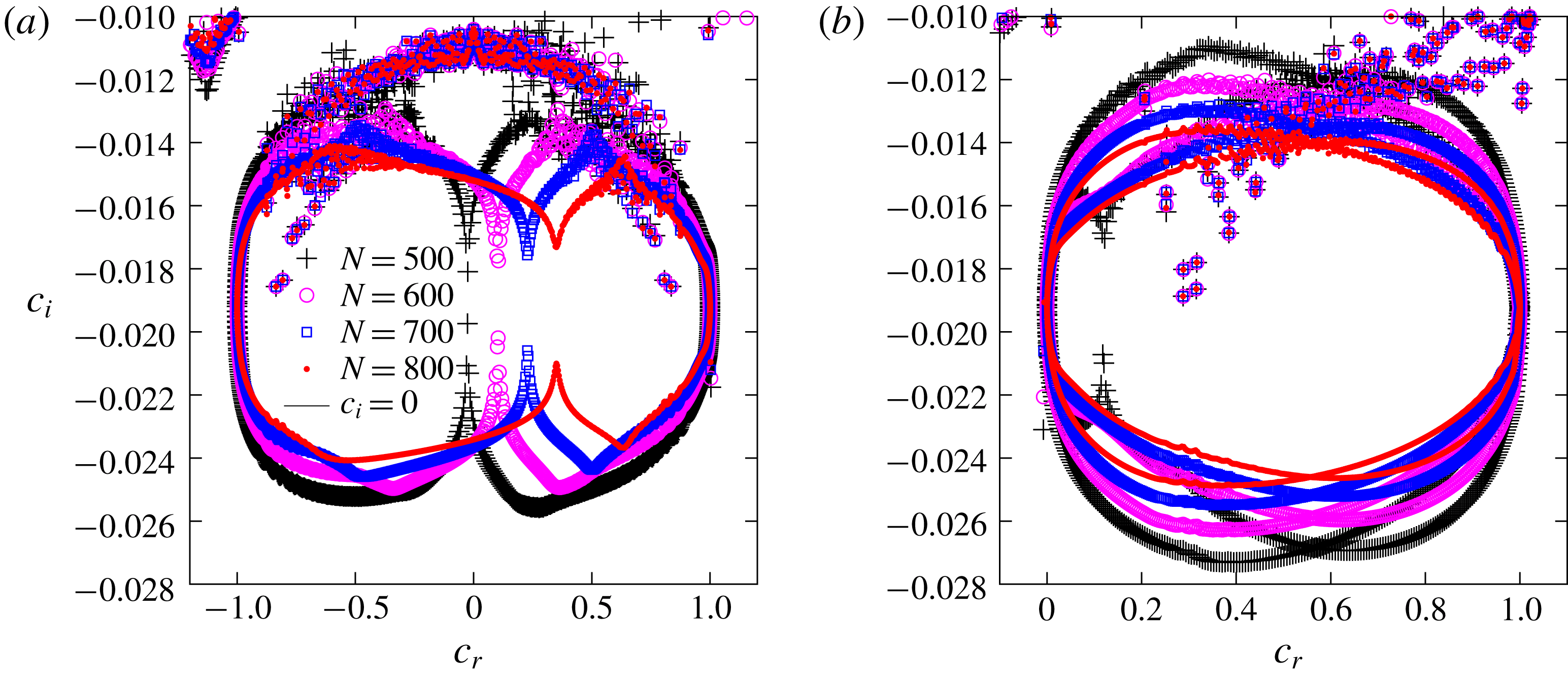
; Graham Reference Graham1998; Sureshkumar Reference Sureshkumar2000) (Author’s paper in preparation: Elastic instability of a vortex column.). Consequently, the spectral method, which uses a finite number of polynomials to approximate the dynamical variables, does not resolve the singular eigenfunctions as accurately as those corresponding to the discrete eigenvalues. The result is a ballooning up of the (expected) ‘line’ of eigenvalues. The spread of the continuous spectrum balloon along the imaginary axis shrinks by a small amount with increase in the number of collocation points
 $N$
(figure 4). Upon filtering (based on a specified tolerance), the balloon disappears with the other unconverged discrete eigenvalues in its vicinity. Inclusion of slow diffusive dynamics of the polymer concentration field (Sureshkumar & Beris Reference Sureshkumar and Beris1995a
; Chokshi & Kumaran Reference Chokshi and Kumaran2009), and thence, of the polymeric stress, introduces non-locality in the constitutive relation thereby regularizing it, in turn leading to the disappearance of the continuous spectrum.
A magnified view of the (unfiltered) continuous spectrum for (a) plane Couette and (b) plane Poiseuille flows for
 $E=0.005,k=2.0,Re=5200$
with
 $N=500$
,
 $600$
,
 $700$
and
 $800$
.

4.1.2 High-frequency Gorodtsov–Leonov modes
The set of discrete eigenvalues in figures 2 and 3 corresponding to the horizontal line
 $c_{i}=-1/(2kW)$
, that appears to extend indefinitely (i.e.
 $c_{r}\rightarrow \pm \infty$
) on either side of the hourglass structure, was first analysed by Gorodtsov & Leonov (Reference Gorodtsov and Leonov1967), and are accordingly termed the HFGL modes. The decay rates of the HFGL eigenmodes are independent of the base velocity profile, with
 $c_{i}=-1/(2kW)$
(Gorodtsov & Leonov Reference Gorodtsov and Leonov1967; Renardy & Renardy Reference Renardy and Renardy1986), although the precise values of the wave speeds (
 $c_{r}$
) are dependent on the velocity profile. The original analysis, for plane Couette flow, was restricted to the limit
 $Re\ll W\sim O(1)$
and
 $\sqrt{ReW}\ll 1$
, in which case
 $c_{r}\sim O(1/\sqrt{ReW})\gg 1$
, with
 $\sqrt{ReW}$
being the viscoelastic Mach number. In dimensional terms,
 $c_{r}\sim O(\sqrt{\unicode[STIX]{x1D702}/(\unicode[STIX]{x1D70C}\unicode[STIX]{x1D706})})\sim O(\sqrt{G/\unicode[STIX]{x1D70C}})\gg U$
, where
 $G$
is the shear modulus of the polymeric liquid. Thus, in the limit analysed, these modes represent a class of weakly damped supersonically propagating shear waves in a viscoelastic fluid. Gorodtsov & Leonov (Reference Gorodtsov and Leonov1967) showed that the
 $n\text{th}$
HFGL eigenvalue is given by
 $c_{i,n}=-1/(2kW)$
, with
 $c_{r,n}=\pm A_{n}/(k\sqrt{ReW})$
, where
 $A_{n}=n\unicode[STIX]{x03C0}/2$
for
 $n\gg 1$
(in the present notation, where we consider the domain
 $z\in [-1,1]$
). Rather interestingly, we find that the expression
 $(n+2)\unicode[STIX]{x03C0}/2$
is a more accurate expression for
 $A_{n}$
, if the HFGL eigenvalue with the lowest
 $|c_{r}|$
is designated to be
 $n=0$
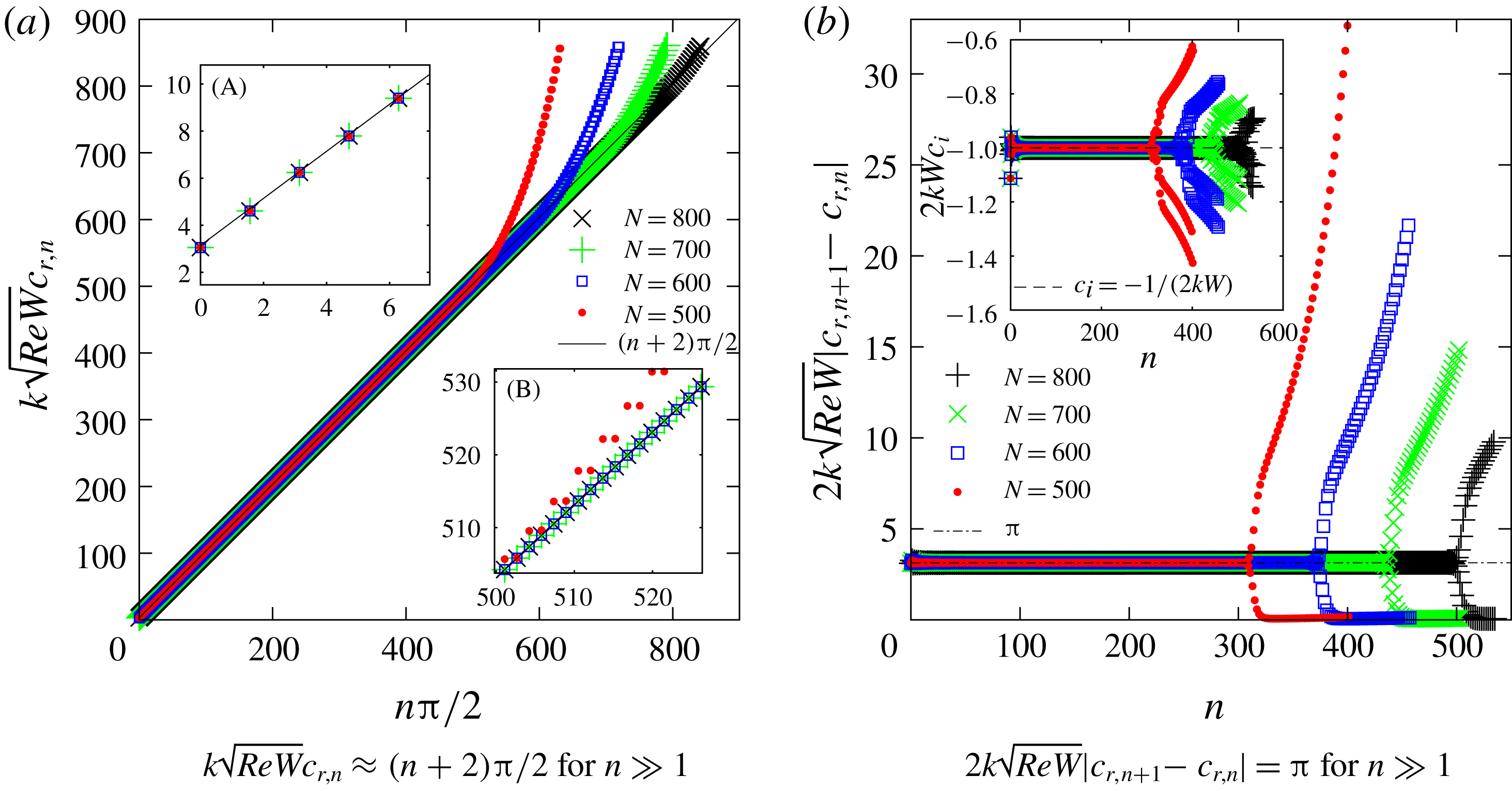
. As shown in figure 5(a), the results from the spectral code (for
 $Re=10^{-4},W=0.9$
) are in excellent agreement with the asymptotic predictions above. Further, figure 5(b) shows that the difference between successive (scaled) eigenvalues approach
 $\unicode[STIX]{x03C0}$
and that
 $c_{i,n}\rightarrow -1/(2kW)$
for higher values of
 $n$
. The numerical results shown in figure 5 splay off the theoretical prediction owing to the invariable loss of convergence (discussed below in more detail) for the higher modes, but this divergence is postponed to a larger value of
 $n$
as
 $N$
increases. The agreement of the difference between successive (scaled) eigenvalues with the theoretical prediction of Gorodtsov & Leonov (Reference Gorodtsov and Leonov1967), on the scale of the plot shown, seems uniformly good for all
 $n$
, although the theoretical prediction is only valid for
 $n\gg 1$
. A zoomed view (not shown) does reveal a discrepancy for the first few values of
 $n$
.
HFGL modes in plane Couette flow for
 $Re=10^{-4},W=0.9$
and
 $k=0.7$
: (a) variation of
 $c_{r}$
with mode number
 $n$
and (b) the absolute value of the difference between successive scaled eigenvalues approaches
 $\unicode[STIX]{x03C0}$
and
 $2kWc_{i,n}\rightarrow -1$
as
 $n\gg 1$
. Inset (A) shows the zoomed view of the region near small values of
 $n$
, and for this case, the estimate,
 $(n+2)\unicode[STIX]{x03C0}/2$
, for the scaled eigenvalue is accurate even for
 $n\sim 1$
. Inset (B) shows the zoomed view of the region where modes splay out for
 $N=500$
. The inset inside panel (b) shows the scaled growth rate versus
 $n$
.

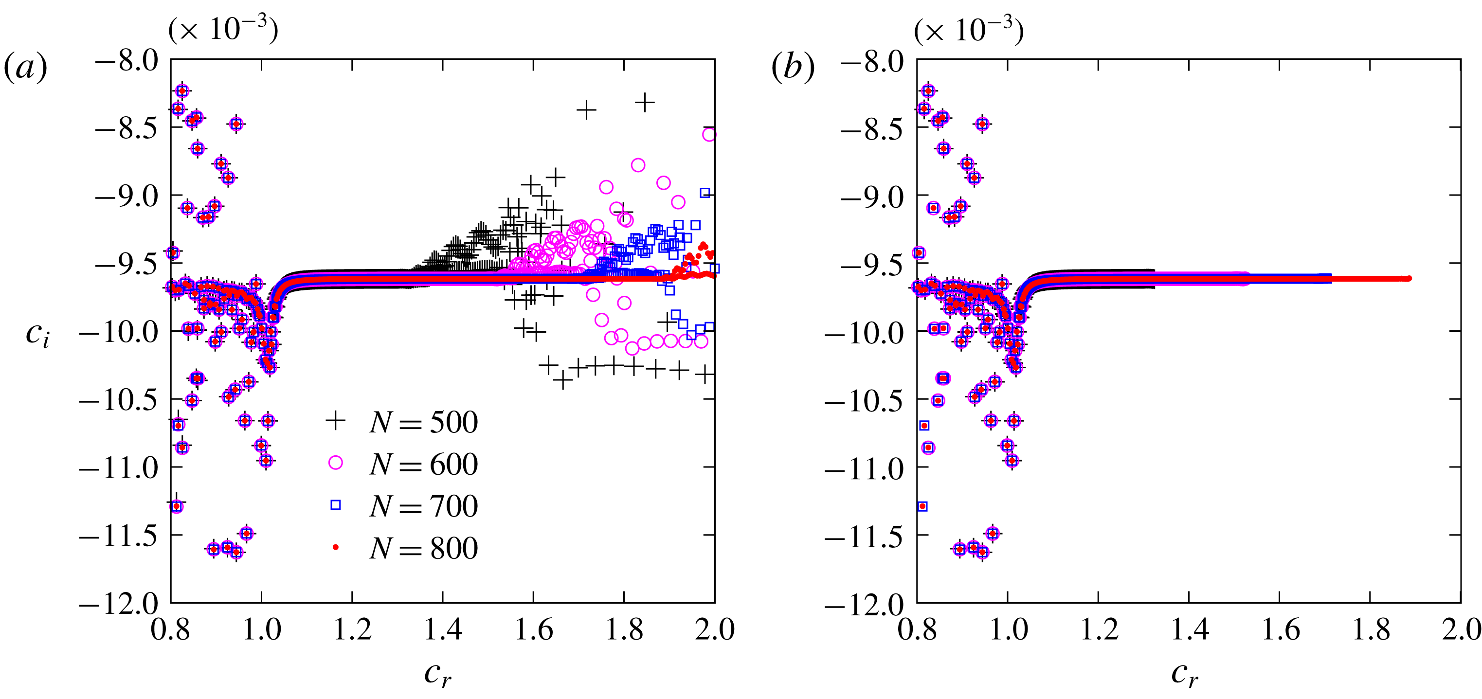
A zoomed view of the HFGL line for plane Poiseuille flow for
 $E=0.005,k=2,Re=5200$
with
 $N=500$
,
 $600$
,
 $700$
and
 $800$
. (a) The unfiltered eigenspectra. (b) The filtered eigenspectra.

Results from the asymptotic analysis of Gorodtsov & Leonov (Reference Gorodtsov and Leonov1967) continue to provide a good approximation to the HFGL part of the spectrum even for
 $Re\gg W\sim O(1)$
, provided
 $A_{n}$
is sufficiently large; such modes still conform to the basic assumption, in the original analysis, of being highly supersonic (i.e.
 $|c|\gg 1$
), and their decay rates are still given by
 $c_{i}=-1/(2kW)$
. This is illustrated most clearly in figure 6 which shows the HFGL part of the eigenspectrum corresponding to figure 3(b), where the Reynolds number (
 $Re=5200$
) is several orders of magnitude larger than that in figure 5, and
 $W=26$
, which explicitly violates the HFGL assumption of
 $Re\ll W$
. This feature is further explored in the following subsection, wherein it is shown that HFGL modes with
 $|c_{r}|\gg 1$
for
 $Re\gg W\sim O(1)$
are well predicted by a WKBJ analysis. Note that although the highly supersonic modes again have decay rates close to
 $c_{i}=-1/(2kW)$
, for
 $c_{r}$
near and in the interval of base-state velocities,
 $c_{i}$
deviates from the aforementioned analytical estimate, and multiple kinks are observed in the HFGL line (figures 2 and 3).
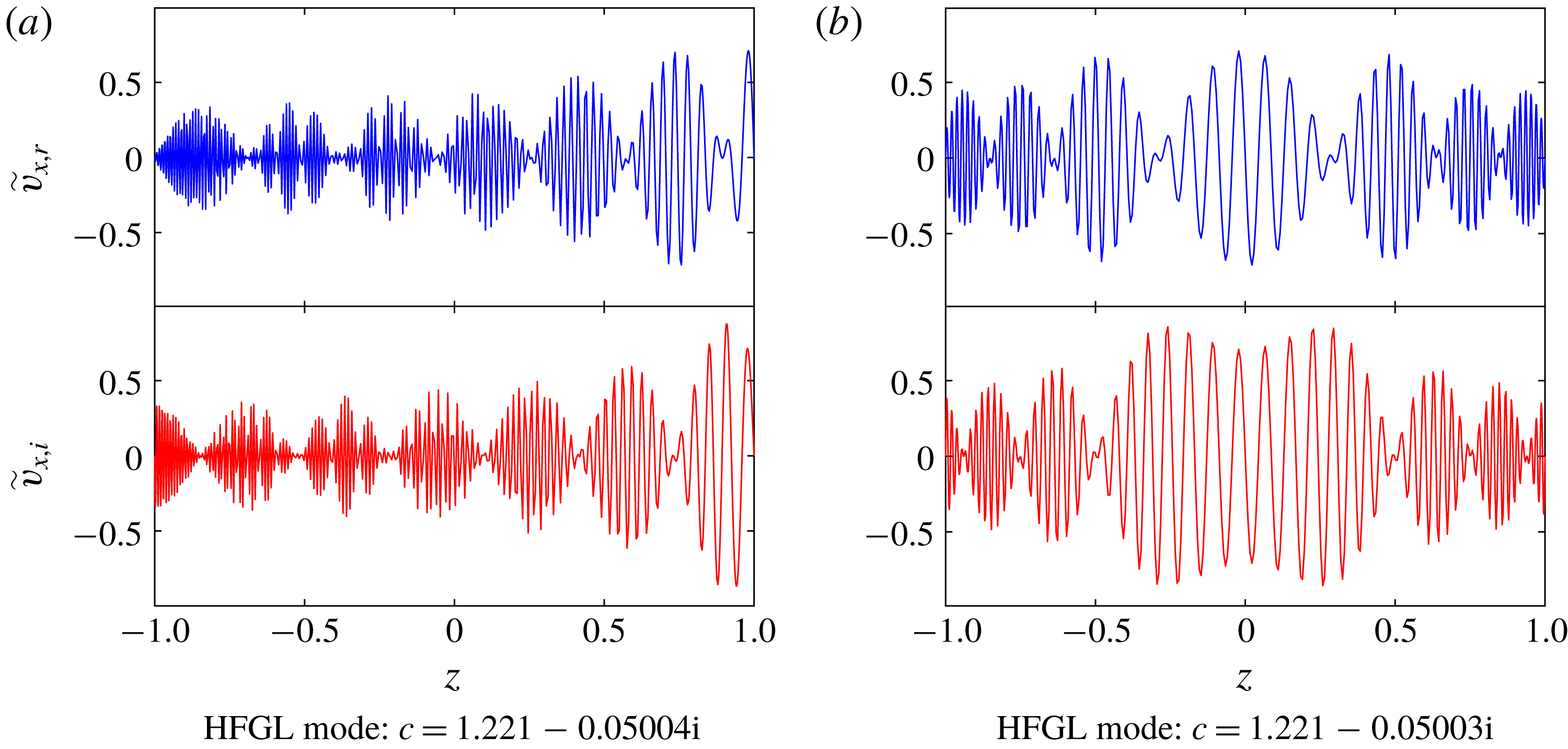
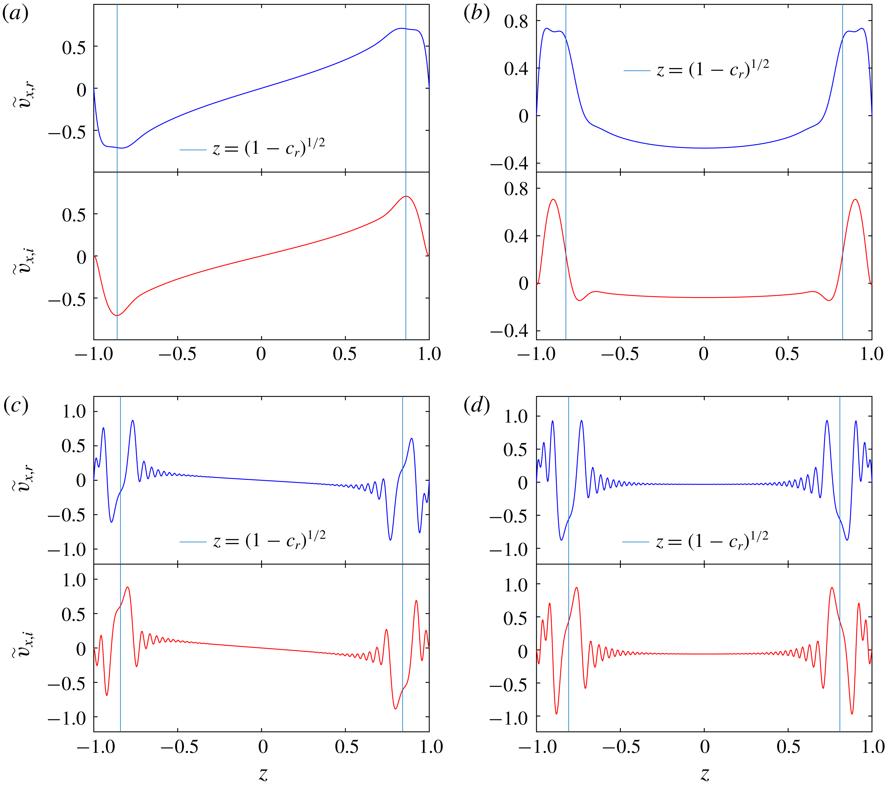
Representative eigenfunctions, corresponding to the HFGL modes from the eigenspectra (figure 2), for plane Couette and Poiseuille flows for
 $Re=10^{4},k=1$
and
 $E=0.001$
are shown in figures 7(a) and 7(b), respectively. In these and the following figures, the eigenfunctions (with real and imaginary parts denoted by the subscripts ‘
 $r$
’ and ‘
 $i$
’, respectively) are normalized so that their maximum absolute value is unity. The eigenfunctions are similar for both the flows and exhibit highly oscillatory behaviour contained within an amplitude envelope that exhibits a secondary longer-wavelength modulation. For both plane Couette and Poiseuille flows, the features in the HFGL eigenfunctions become increasingly fine grained with increase in
 $|c_{r}|$
(figure not shown). The fine-scaled oscillations cause the eigenvalues with higher
 $|c_{r}|$
to splay out from their analytical estimates of
 $c_{i}=-1/(2kW)$
(figure 6
a) for a given number of collocation points
 $N$
. The smallest length scale resolved is limited by the chosen value of
 $N$
, and HFGL modes with
 $c_{r}$
higher than an
 $N$
-dependent threshold cannot be predicted accurately. Equivalently, in figure 6(b), the greater horizontal ‘extent’ of the HFGL line for higher
 $N$
illustrates the improved resolution of the fine-scaled higher
 $|c_{r}|$
modes.
Real and imaginary parts of normalized
 $x$
-velocity eigenfunctions corresponding to the HFGL modes in (a) plane Couette flow, and (b) plane Poiseuille flow for
 $E=0.001,k=1,Re=10^{4}$
and
 $N=500$
. These eigenfunctions correspond to eigenvalues that belong to the eigenspectra shown in figures 2(a) and 2(b), respectively.

4.1.3 Asymptotic analysis of HFGL modes at high
 $Re$

The governing linearized momentum and constitutive relations (3.8)–(3.13) are combined to yield a single fourth-order differential equation for the wall-normal velocity,
 $\tilde{v}_{z}$
, by eliminating the other independent fields,
 $$\begin{eqnarray}\displaystyle & & \displaystyle \mathscr{D}^{4}\tilde{v}_{z}+\mathscr{D}^{3}\tilde{v}_{z}(2\text{i}kWU^{\prime }-2U^{\prime }\unicode[STIX]{x1D6F4}^{-1})\nonumber\\ \displaystyle & & \displaystyle \quad +\,\mathscr{D}^{2}\tilde{v}_{z}(-2k^{2}(1+W^{2}(U^{\prime })^{2})+3\text{i}kWU^{\prime \prime }-\unicode[STIX]{x1D6F4}^{-1}(4\text{i}kW(U^{\prime })^{2}+3U^{\prime \prime })+2\unicode[STIX]{x1D6F4}^{-2}(U^{\prime })^{2})\nonumber\\ \displaystyle & & \displaystyle \quad +\,\mathscr{D}\tilde{v}_{z}(-2\text{i}k^{3}WU^{\prime }+8k^{2}W^{2}U^{\prime }U^{\prime \prime }-\unicode[STIX]{x1D6F4}^{-1}(2k^{2}(1-2U^{\prime }-2W^{2}(U^{\prime })^{3})+8\text{i}kWU^{\prime \prime }U^{\prime })\nonumber\\ \displaystyle & & \displaystyle \quad +\,\text{i}k^{-1}\unicode[STIX]{x1D6F4}^{-2}(4k^{2}W(U^{\prime })^{3}-4\text{i}kU^{\prime \prime }U^{\prime }))\nonumber\\ \displaystyle & & \displaystyle \quad +\,\tilde{v}_{z}\left(-\text{i}k(\text{i}k^{3}+2\text{i}k^{3}W^{2}(U^{\prime })^{2}+4\text{i}kW^{2}(U^{\prime \prime })^{2}+4\text{i}kW^{2}U^{\prime \prime \prime }U^{\prime }-8\text{i}kU^{\prime \prime }U^{\prime }+k^{2}WU^{\prime \prime })\right.\nonumber\\ \displaystyle & & \displaystyle \quad -\,\unicode[STIX]{x1D6F4}^{-1}(2\text{i}k^{3}WU^{\prime }(1-U^{\prime })+\text{i}kU^{\prime \prime }(\text{i}k+2\text{i}kW^{2}(U^{\prime })^{2}+3WU^{\prime \prime }))\nonumber\\ \displaystyle & & \displaystyle \quad \left.+\,\text{i}k^{-1}\unicode[STIX]{x1D6F4}^{-2}(2k^{2}(U^{\prime })^{2}(\text{i}k+2\text{i}kW^{2}(U^{\prime })^{2}+WU^{\prime \prime })+4k^{2}WU^{\prime \prime }(U^{\prime })^{2})\right)\nonumber\\ \displaystyle & & \displaystyle =-k^{2}ReW(U-c)\unicode[STIX]{x1D6F4}((\mathscr{D}^{2}-k^{2})\tilde{v}_{z}+U^{\prime \prime }(U-c)^{-1}\tilde{v}_{z}),\end{eqnarray}$$
where
 $\unicode[STIX]{x1D6F4}=U-c-\text{i}k^{-1}W^{-1}.$
We consider here the limit
 $Re\gg 1$
, and define the small parameter
 $\unicode[STIX]{x1D716}=1\!/\!(\text{i}k(ReW)^{1/2})\ll 1$
in the ensuing analysis. In this limit, to achieve a dominant balance between the inertial, viscous and elastic forces, it is necessary to rescale the lengths using
 $O(ReW)^{-1/2}\ll 1$
, implying that we look for rapidly varying solutions, on the length scale of
 $(ReW)^{-1/2}$
, using the WKBJ ansatz (Lin Reference Lin1945; Drazin & Reid Reference Drazin and Reid2004; Bender & Orszag Reference Bender and Orszag2013) ansatz, as follows:
 $$\begin{eqnarray}\displaystyle & \displaystyle \tilde{v}_{z}=\exp \left(\int g\,\text{d}z\right), & \displaystyle\end{eqnarray}$$
with
 $$\begin{eqnarray}\displaystyle & \displaystyle g=g_{0}/\unicode[STIX]{x1D716}+g_{1}+g_{2}\unicode[STIX]{x1D716}+\cdots \,. & \displaystyle\end{eqnarray}$$
The equation governing
 $\tilde{v}_{z}$
to
 $O(1)$
in (4.3) can be derived from (4.1) and is given by,
 $$\begin{eqnarray}\displaystyle \unicode[STIX]{x1D716}^{2}(\mathscr{D}^{4}\tilde{v}_{z}+\mathscr{D}^{3}\tilde{v}_{z}(2\unicode[STIX]{x1D716}^{-1}U^{\prime }E^{1/2}-2U^{\prime }\unicode[STIX]{x1D6F4}^{-1}))=\mathscr{D}^{2}\tilde{v}_{z}((U-c)\unicode[STIX]{x1D6F4}-2(U^{\prime })^{2}E). & & \displaystyle\end{eqnarray}$$
Substituting equation (4.3) in (4.4), then leads to the following expression for
 $\tilde{v}_{z}$
:
 $$\begin{eqnarray}\displaystyle \tilde{v}_{z} & = & \displaystyle {\displaystyle \frac{1}{((U-c)\unicode[STIX]{x1D6F4}-(U^{\prime })^{2}E)^{1/2}(-U^{\prime }E^{1/2}\pm ((U-c)\unicode[STIX]{x1D6F4}-(U^{\prime })^{2}E)^{1/2})^{2}}}\nonumber\\ \displaystyle & & \displaystyle \quad \exp \left(\unicode[STIX]{x1D716}^{-1}E^{1/2}U\pm \text{i}k\unicode[STIX]{x1D716}^{-1}\int ((U-c)\unicode[STIX]{x1D6F4}-E(U^{\prime })^{2})^{1/2}\,\text{d}z\right.\nonumber\\ \displaystyle & & \displaystyle \quad \left.+\int U^{\prime }g_{0}\unicode[STIX]{x1D6F4}^{-1}(g_{0}+U^{\prime }E^{1/2})^{-1}\,\text{d}z\right),\end{eqnarray}$$
where
 $$\begin{eqnarray}\displaystyle g_{0}=-U^{\prime }E^{1/2}\pm ((U-c)\unicode[STIX]{x1D6F4}-(U^{\prime })^{2}E)^{1/2}. & & \displaystyle\end{eqnarray}$$
Using continuity, we obtain the following expression for the axial velocity, simplified to the leading order in
 $\unicode[STIX]{x1D716}$
and
 $E^{1/2}$
:
 $$\begin{eqnarray}\displaystyle \tilde{v}_{x}={\displaystyle \frac{\unicode[STIX]{x1D716}^{-1}}{((U-c)\unicode[STIX]{x1D6F4})^{3/2}}}\exp \left(\unicode[STIX]{x1D716}^{-1}E^{1/2}U\pm \unicode[STIX]{x1D716}^{-1}\int (U-c)^{1/2}\unicode[STIX]{x1D6F4}^{1/2}\,\text{d}z\right)+O(\unicode[STIX]{x1D716})+O(E^{1/2}). & & \displaystyle \nonumber\\ \displaystyle & & \displaystyle\end{eqnarray}$$
Owing to the small transverse length scale, the flow associated with these elasto-inertial eigenfunctions is a nearly unidirectional flow, with a dominant tangential component. One therefore needs to satisfy only the no-slip condition for
 $v_{x}$
at leading order. Using the boundary conditions for
 $\tilde{v}_{x}$
, then leads to the following dispersion relation for
 $(ReW)^{1/2}\gg 1$
and
 $E^{1/2}\ll 1$
:
 $$\begin{eqnarray}\displaystyle k(ReW)^{1/2}\int _{-1}^{1}(U-c)^{1/2}\unicode[STIX]{x1D6F4}^{1/2}\,\text{d}z=n\unicode[STIX]{x03C0}. & & \displaystyle\end{eqnarray}$$
The above (4.8) is solved by
 $c=c_{r}+\text{i}c_{i}$
, where
 $c_{i}=-1/(2kW)$
and
 $$\begin{eqnarray}\displaystyle \int _{-1}^{1}\left((U-c_{r})^{2}+{\displaystyle \frac{1}{(2kW)^{2}}}\right)^{1/2}\,\text{d}z={\displaystyle \frac{n\unicode[STIX]{x03C0}}{k(ReW)^{1/2}}}. & & \displaystyle\end{eqnarray}$$
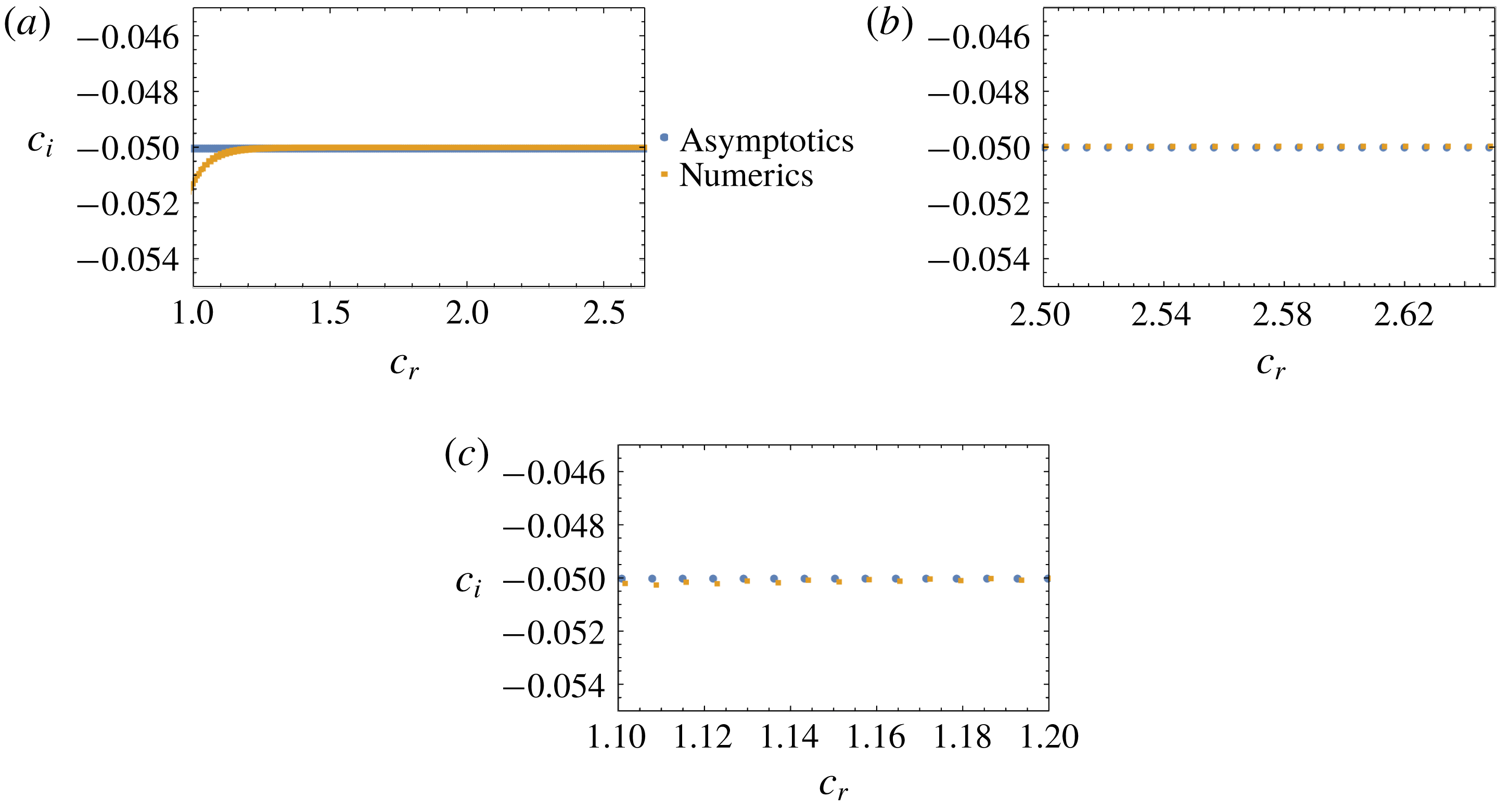
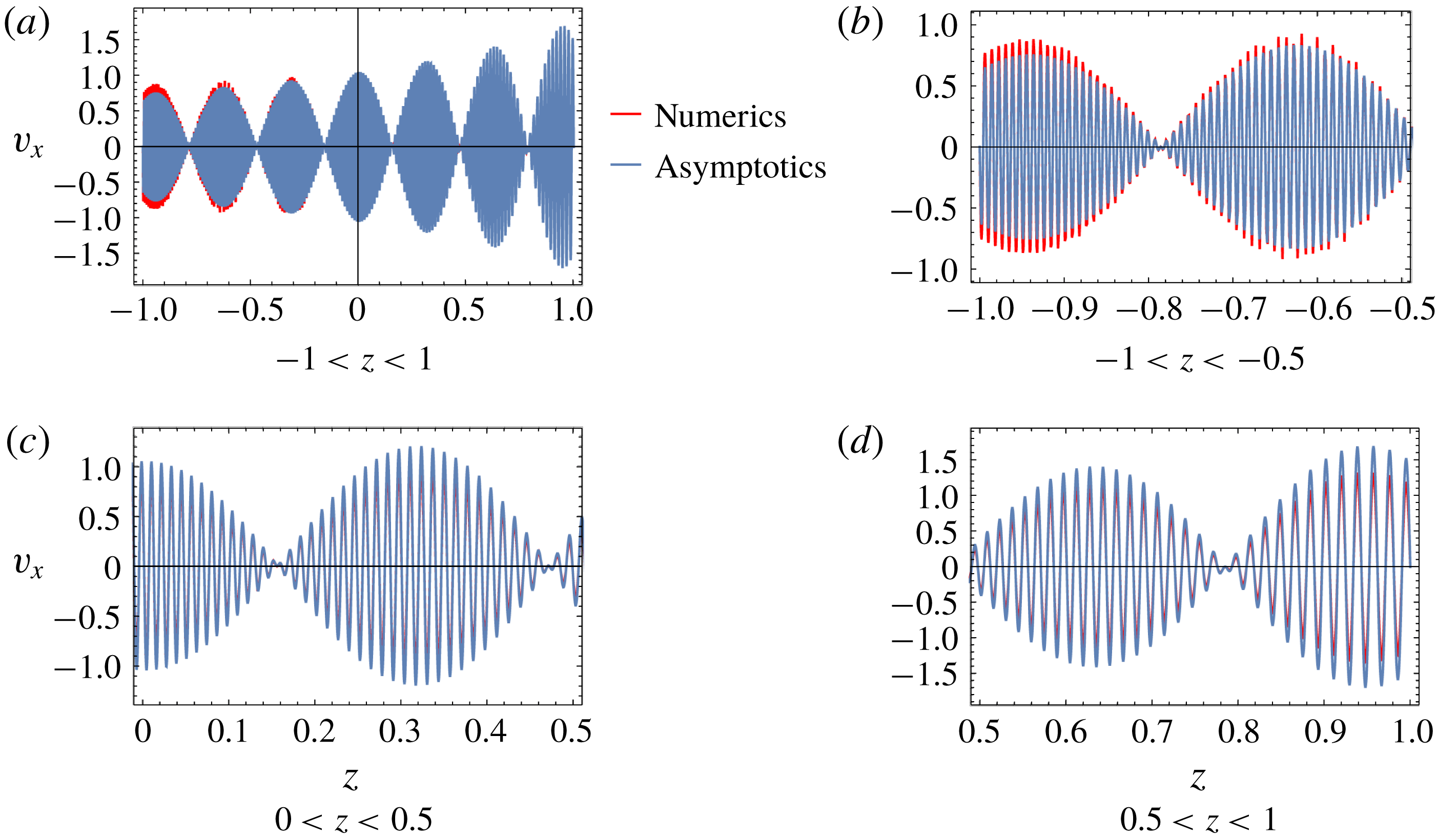
Figures 8 and 9 reveal a good comparison between the numerical and asymptotic results. In our analysis, we have assumed that (4.5) is valid throughout the domain which requires that the singularities of the expression are well away from the real axis. This is true for
 $|c_{r}|>1$
. When
 $|c_{r}|<1$
, there is a critical layer in the channel where (4.5) breaks down and a matched-asymptotic analysis with an inner turning point region is required (Lin Reference Lin1945; Drazin & Reid Reference Drazin and Reid2004; Bender & Orszag Reference Bender and Orszag2013) to accurately capture the eigenvalues. This is reflected in figures 8(a) and 8(c), where the differences between asymptotic and numerical results become substantial as
 $c_{r}\rightarrow 1$
.
Comparison of the eigenvalues for the HFGL part of the spectrum obtained from the asymptotic expression with the numerically obtained eigenvalue for
 $Re=5000,W=10,k=1$
for Couette flow;
 $1500$
collocation points were taken for the numerics. (a)
 $1<c_{r}<2.6$
. (b)
 $c_{r}\sim 2.5$
. (c)
 $c_{r}\sim 1.1$
.

Comparison of the axial velocity eigenfunctions from the asymptotic analysis and the numerical solution for the HFGL eigenvalue
 $c_{r}=2.458$
and
 $Re=5000,W=10,k=1$
for Couette flow;
 $1500$
collocation points were taken for the numerics. While panel (a) shows the entire domain, the other panels (b–d) zoom into smaller intervals to show the rapid oscillations more clearly.

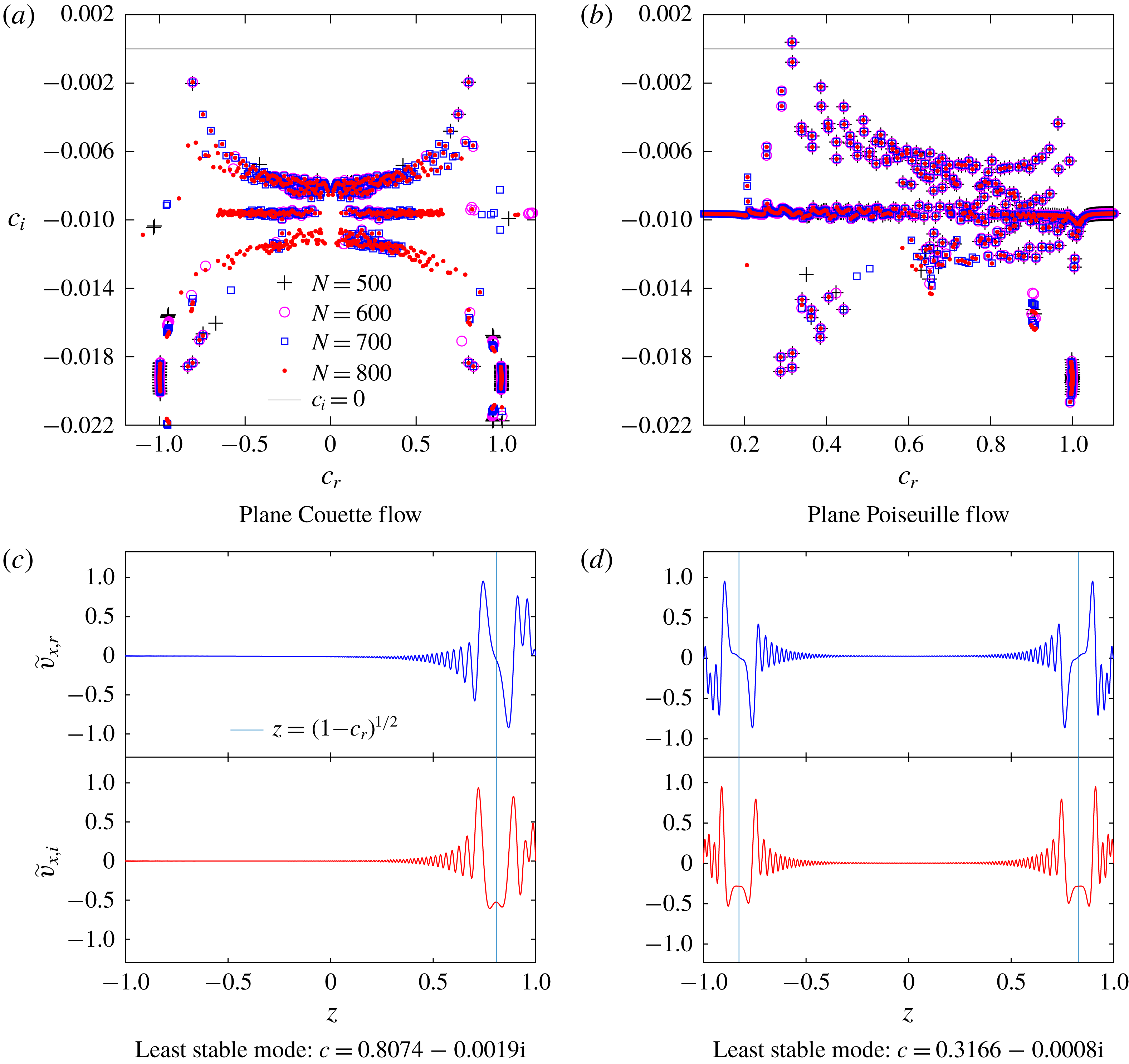
Filtered eigenspectra illustrating the hourglass modes for (a) plane Couette flow, and (b) plane Poiseuille flow for
 $E=0.005,k=2,Re=5200$
with
 $N=500$
,
 $600$
,
 $700$
and
 $800$
, and normalized
 $x$
-velocity eigenfunctions corresponding to the least stable modes for (c) plane Couette flow in panel (a) and (d) plane Poiseuille flow in panel (b).

4.1.4 Hourglass modes
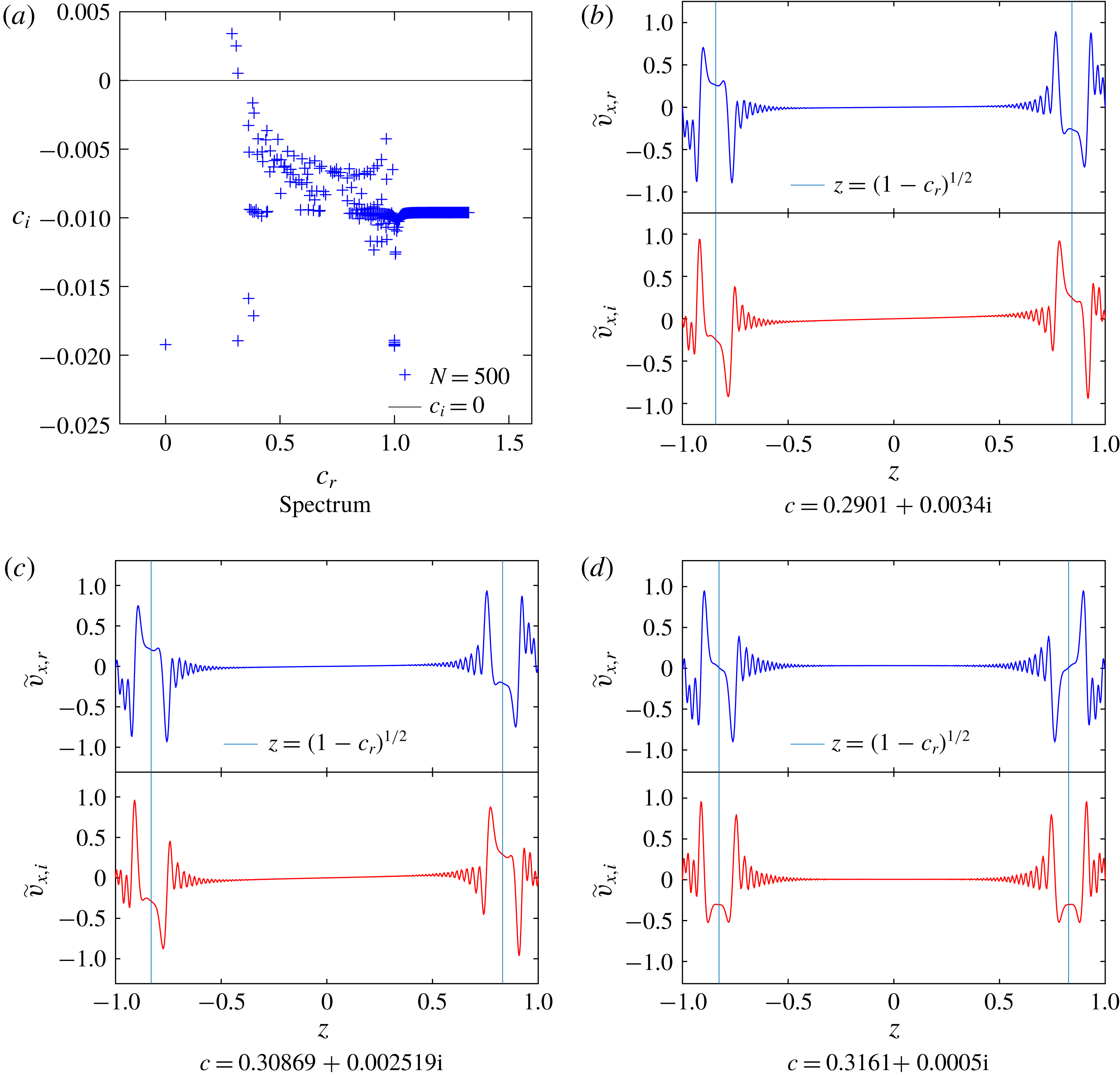
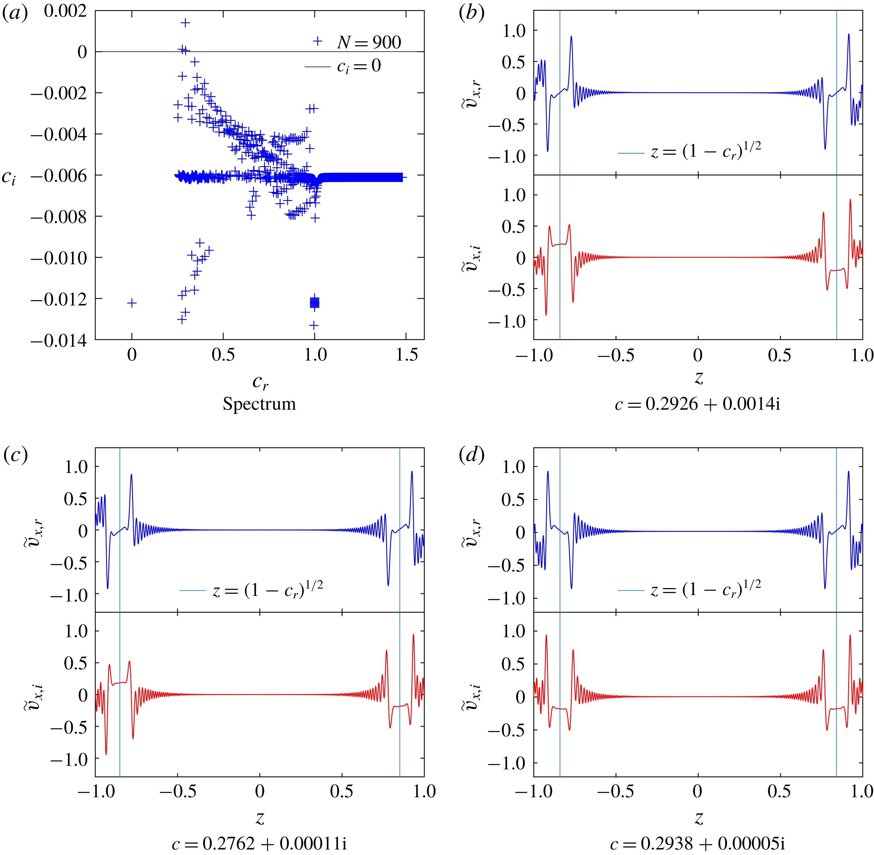
As seen in figures 2 and 3 (depicting unfiltered spectra), and in figures 10(a) and 10(b) (depicting filtered spectra), the HFGL line lies between the two ‘bulbs’ of an (approximately) hourglass-shaped structure in the interval
 $c_{r}\in [0,1]$
, for both plane Couette and Poiseuille flows. It is necessary to plot (as in figure 10) the filtered spectra for parametric regimes in which the ballooned up continuous spectrum tends to mask the physically genuine eigenvalues belonging to the lower bulb of the hourglass structure. The hourglass structure is expectedly symmetric about
 $c_{r}=0$
for plane Couette flow, but is not for plane Poiseuille flow where fewer eigenvalues are present for
 $c_{r}$
close to
 $1$
compared to
 $c_{r}$
close to zero. The lower bulb of the hourglass lies between the HFGL line (
 $c_{i}=-1/(2kW)$
) and the continuous spectrum (
 $c_{i}=-1/(kW)$
). The upper bulb lies between the HFGL line and the
 $c_{i}=0$
axis for plane Couette flow, while for plane Poiseuille flow, the low-
 $c_{r}$
branch of the upper bulb crosses the
 $c_{i}=0$
line, leading to instabilities. In figures 10(a) and 10(b), a higher value of
 $N$
(
 ${\sim}800$
) is required to capture the lower bulb of the hourglass compared to that required (
 $N\sim 500$
) for the upper bulb, due to the encroachment of the lower bulb by the ballooned-up continuous spectrum. Indeed, only at
 $N=800$
, is the lower bulb of the hour glass structure reasonably complete in figure 10(a) for plane Couette flow, and is beginning to get populated in figure 10(b) for plane Poiseuille flow.
The eigenfunctions corresponding to the least stable eigenvalues in the upper bulb of the hourglass structure are shown in figures 10(c) and 10(d). While the oscillations of the HFGL eigenfunctions (in figure 7) span the entire channel domain, those for the least stable hourglass modes exhibit localized large-amplitude oscillations close to the wall. However, as we proceed down the hourglass structure to modes with
 $c_{r}\sim 0$
(for plane Couette) or
 $c_{r}\sim 0.5$
(for plane Poiseuille), there is a gradual transition in the structure of the eigenfunctions from wall-localized oscillations (characteristic of the least stable or unstable modes; see § 4.2 for the eigenfunctions corresponding to the unstable mode) to de-localized oscillations similar to the (stable) HFGL modes. The maximum amplitude of the hourglass eigenfunctions occurs in the vicinity of the critical point
 $z_{c}=(1-c_{r})^{1/2}$
where the phase speed
 $c_{r}$
equals the local base-flow velocity indicated by a vertical line in figures 10(c) and 10(d). The least stable eigenfunctions of the hourglass structure are wall modes with phase velocities
 $c_{r}\rightarrow \pm 1$
(for plane Couette flow) and
 $c_{r}\ll 1$
(for plane Poiseuille flow) in the limit of
 $Re\gg 1$
(Schmid & Henningson Reference Schmid and Henningson2001). As mentioned above, and discussed in more detail below, it is the wall modes belonging to the upper bulb of the hourglass that turn unstable in plane Poiseuille flow as
 $Re$
and
 $E$
are increased.
4.1.5 Evolution of the elasto-inertial eigenspectrum with
$E$

Figure 11(a) shows the Newtonian eigenspectrum for plane Couette flow (
 $E=0$
) which has the familiar Y-shaped structure with three distinct branches (Schmid & Henningson Reference Schmid and Henningson2001). Following Mack (Reference Mack1976), and as mentioned (briefly) at the beginning of this section, we label the vertical branch with phase speeds equal to the average velocity of the base flow (
 $c_{r}=0$
) as the ‘
 $S$
’-branch, and the two symmetrical arms of the Y-shaped spectrum consisting of modes, with
 $c_{r}$
progressively approaching the velocity of the two walls, as the ‘
 $A$
’-branches. The
 $S$
-branch in Newtonian plane Couette flow extends down to
 $c_{i}=-\infty$
. In figure 11(a) there is a region at the intersection of the three branches where the eigenvalues are not convergent. This lack of convergence is well known, and has been attributed to non-orthogonality of the eigenvectors, which renders the eigenspectrum in that region very sensitive to numerical (round-off or truncation) errors in the discretized linear operator (Schmid & Henningson Reference Schmid and Henningson2001).
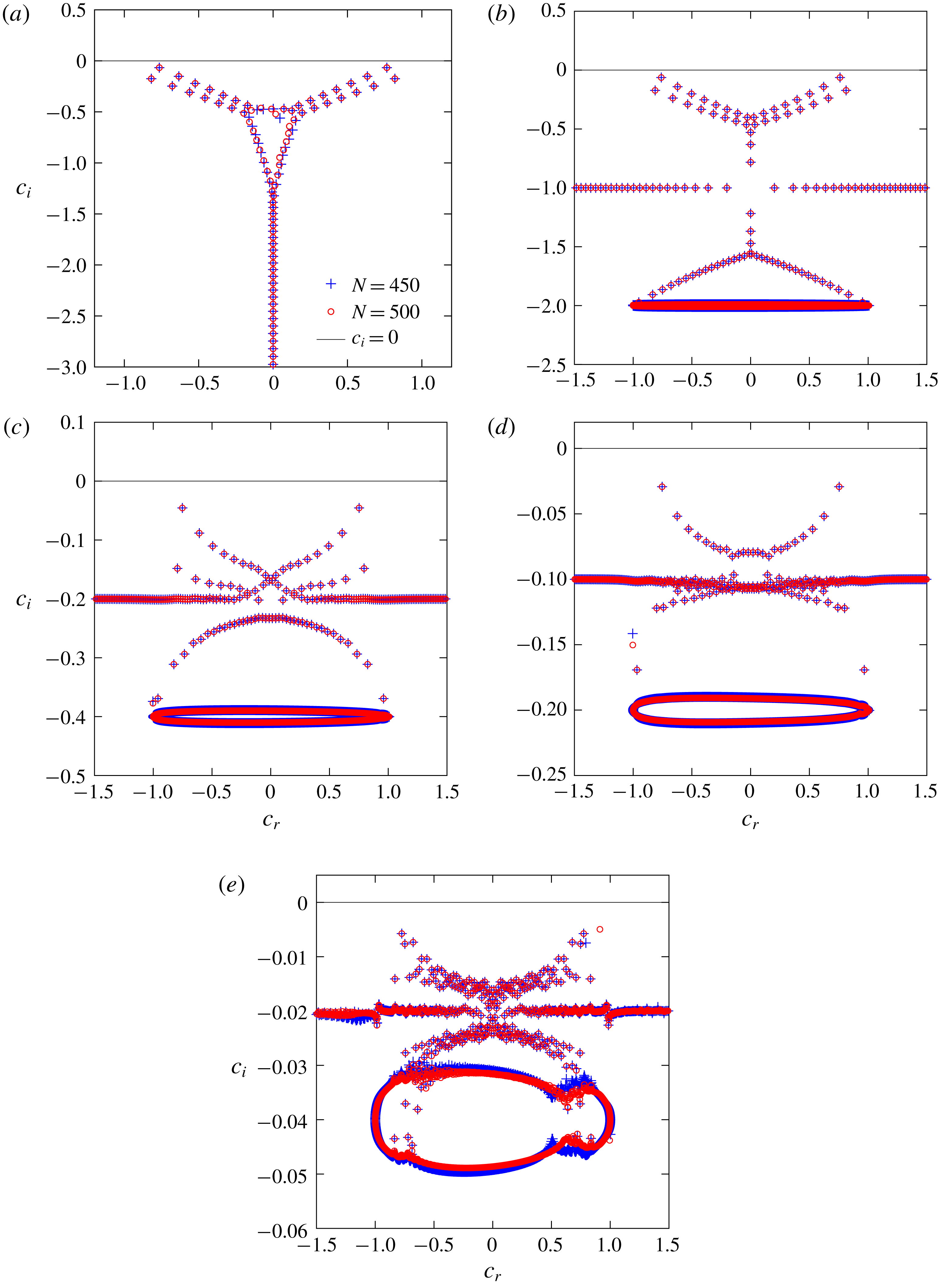
Evolution of the eigenspectrum for plane Couette flow with increase in
 $E$
: unfiltered eigenspectrum for
 $N=450$
and
 $500$
for (a) Newtonian fluid (
 $E=0$
), (b)
 $E=10^{-4}$
, (c)
 $E=5\times 10^{-4}$
, (d)
 $E=10^{-3}$
and (e)
 $E=5\times 10^{-3}$
, for
 $Re=5000$
and
 $k=1$
.

The Newtonian limit of
 $E\rightarrow 0$
is a singular one, so even for
 $E\ll 1$
, in sharp contrast to the Newtonian spectrum, the vertical extent of the elasto-inertial UCM spectrum is finite (of
 $O(1/E)$
), because the fastest relaxation is limited by the intrinsic relaxation time of the polymer. Thus, as shown in figures 11(a)–11(e), as
 $E$
is increased for a fixed
 $Re$
, the extent of the eigenspectrum along the
 $c_{i}$
-axis decreases as
 $1/E$
. An inverted Y-structure also appears below the truncated
 $S$
-branch ending in the continuous spectrum balloon. The HFGL modes are evidently absent for
 $E=0$
. For any non-zero
 $E$
, the HFGL line appears midway between the Y and inverted Y structures (figure 11
b). Figures 11(b)–11(e) show that for increasing values of
 $E$
the upper and lower Y structures gradually transform to the approximately hourglass-shaped structure mentioned earlier, with the vertical extent of this structure again shrinking with increasing
 $E$
(and
 $k$
; figures 11
b–11
e). In addition, the ballooned-up continuous spectrum expands along
 $c_{i}$
-axis with increase in
 $E$
, presumably because the eigenfunctions for the polymer stress components becoming more singular with increasing
 $E$
. The hourglass structure is found to have more eigenvalues for higher
 $E$
, but none of these modes become unstable for plane Couette flow. A similar, but not identical, scenario prevails for the plane Poiseuille spectrum. In this case, however, as
 $E$
is increased, the modes along the low-
 $c_{r}$
branch eventually become unstable; the modes along the high-
 $c_{r}$
branch remain stable. The unstable wall modes above are discussed in more detail in the next section.
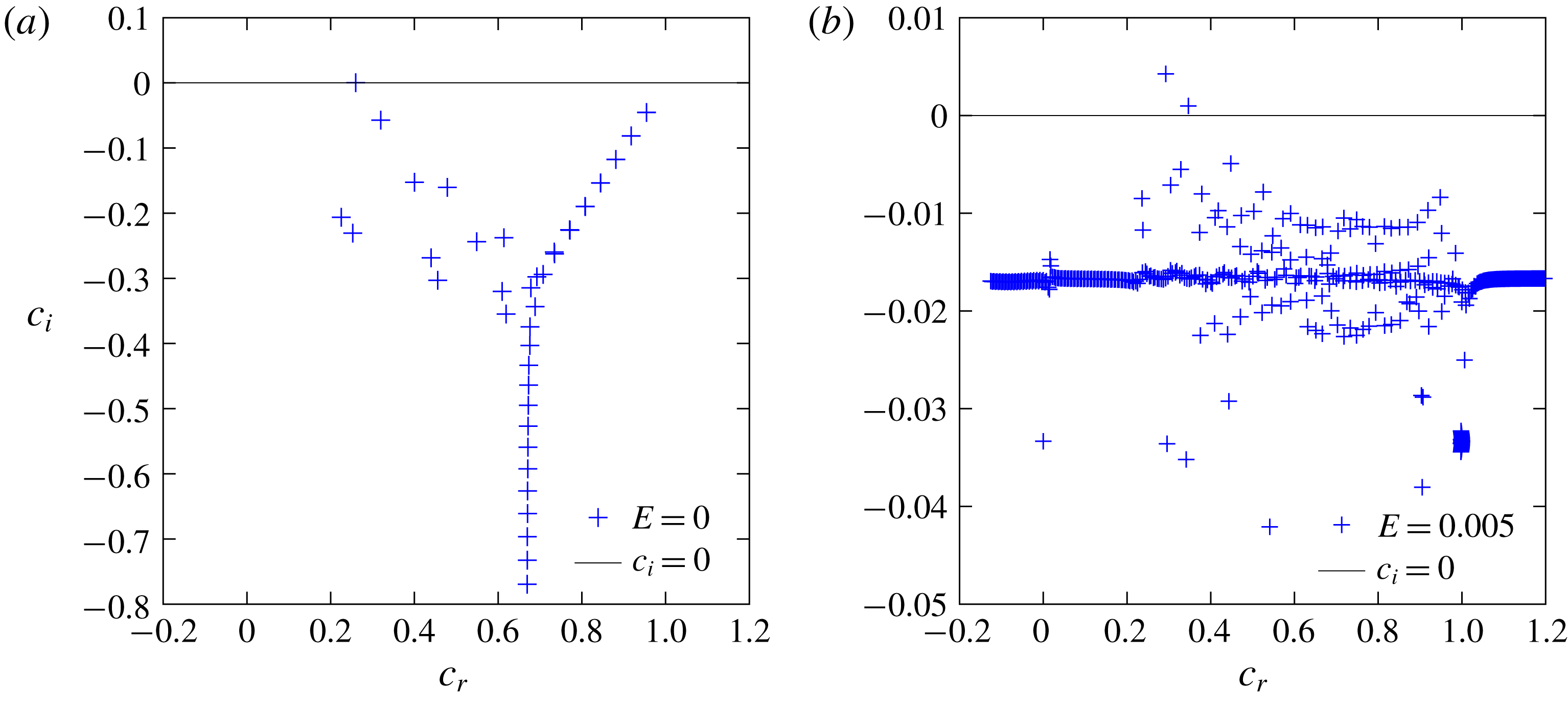
Spectrum for plane Poiseuille flow for Newtonian (
 $E=0$
) and Oldroyd-B (
 $E=0.005$
) fluids:
 $Re=6000$
and
 $k=1$
. For the Newtonian fluid, there is only one unstable (antisymmetric) mode. For the UCM fluid, there are two unstable modes, with the most unstable mode (
 $A1(b)$
) being antisymmetric and the other mode being symmetric (
 $S1$
). (a) Newtonian,
 $E=0$
. (b) UCM,
 $E=0.005$
.

4.2 Instabilities in plane Poiseuille flow
Normalized eigenfunctions for the
 $x$
-velocity corresponding to the eigenmodes found for plane Poiseuille flow for the parameters
 $k=1,Re=6000$
and
 $N=500$
. (a) Antisymmetric eigenfunction for Newtonian fluid (
 $E=0$
) corresponding to the unstable eigenvalue
 $0.259815871+0.000323089\text{i}$
, (b) symmetric eigenfunction for Newtonian fluid (
 $E=0$
) corresponding to the stable eigenvalue
 $0.319582136-0.057148151\text{i}$
, (c) antisymmetric eigenfunction for UCM fluid (
 $E=0.005$
) corresponding to the unstable
 $A1(b)$
mode
 $0.292643237+0.004260020\text{i}$
and (d) symmetric eigenfunction for the UCM fluid (
 $E=0.005$
) corresponding to the unstable
 $S1$
mode
 $0.346547248+0.000983114\text{i}$
.

Structure of the unstable modes in the physical
 $x$
–
 $z$
plane for
 $Re=6000$
,
 $k=1$
and
 $N=500$
. (a) For mode
 $A1(a)$
with
 $E=5\times 10^{-4}$
and
 $c=0.26212758+0.0081117\text{i}$
, and (b) for mode
 $A1(b)$
with
 $E=0.005$
,
 $c=0.292643237+0.00426002\text{i}$
. The location of the critical layer is shown using white dashed lines.

An extensive search in parameter space over the range
 $0<Re\leqslant 10^{4}$
,
 $0<E\leqslant 0.01$
and
 $0<k\leqslant 5$
did not show any instability for plane Couette flow of a UCM fluid, in accordance with the earlier conclusions of Renardy & Renardy (Reference Renardy and Renardy1986). For viscoelastic plane Poiseuille flow, however, the search revealed the modified TS instability, and a whole new hierarchy (possibly, an infinite one) of unstable elasto-inertial modes. The unstable eigenvalues always occur as part of the left branch of the upper bulb in the hourglass structure. The eigenspectrum for plane Poiseuille flow for
 $k=1,Re=6000$
shows one unstable eigenmode (the TS mode) for a Newtonian fluid (
 $E=0$
) but two unstable ones for a UCM fluid at
 $E=0.005$
(figures 12
a and 12
b). The corresponding eigenfunctions for the streamwise disturbance velocity
 $\tilde{v}_{x}$
are shown in figure 13. It is well known that the unstable TS-mode (the streamwise velocity eigenfunction thereof) in a Newtonian fluid is antisymmetric (figure 13
a) (Orszag & Kells Reference Orszag and Kells1980). The least stable symmetric eigenfunction for the Newtonian case is shown in figure 13(b) for the same set of parameters. Both eigenfunctions have a single extremum near the wall and decay smoothly towards the centreline. At
 $E=0.005$
, for the same
 $Re$
and
 $k$
, we find that both antisymmetric and symmetric eigenmodes become unstable, unlike the Newtonian case. The eigenfunctions for the unstable eigenvalues, shown in figures 13(c) and 13(d) respectively, exhibit a fine-scaled oscillatory structure, with the amplitude decaying towards the centreline, the oscillatory structure being indicative of the importance of elasto-inertial effects. These features are similar to those for the stable eigenfunctions belonging to the hourglass structure shown, for example, in figure 10(d), but are qualitatively different from those (figure 7) of the HFGL modes which have
 $|c_{r}|>1$
. It is worth noting that the instability of a symmetric eigenmode has not been reported in the existing literature on the stability of viscoelastic channel flows (Porteous & Denn Reference Porteous and Denn1972; Lee & Finlayson Reference Lee and Finlayson1986; Sureshkumar & Beris Reference Sureshkumar and Beris1995b
).
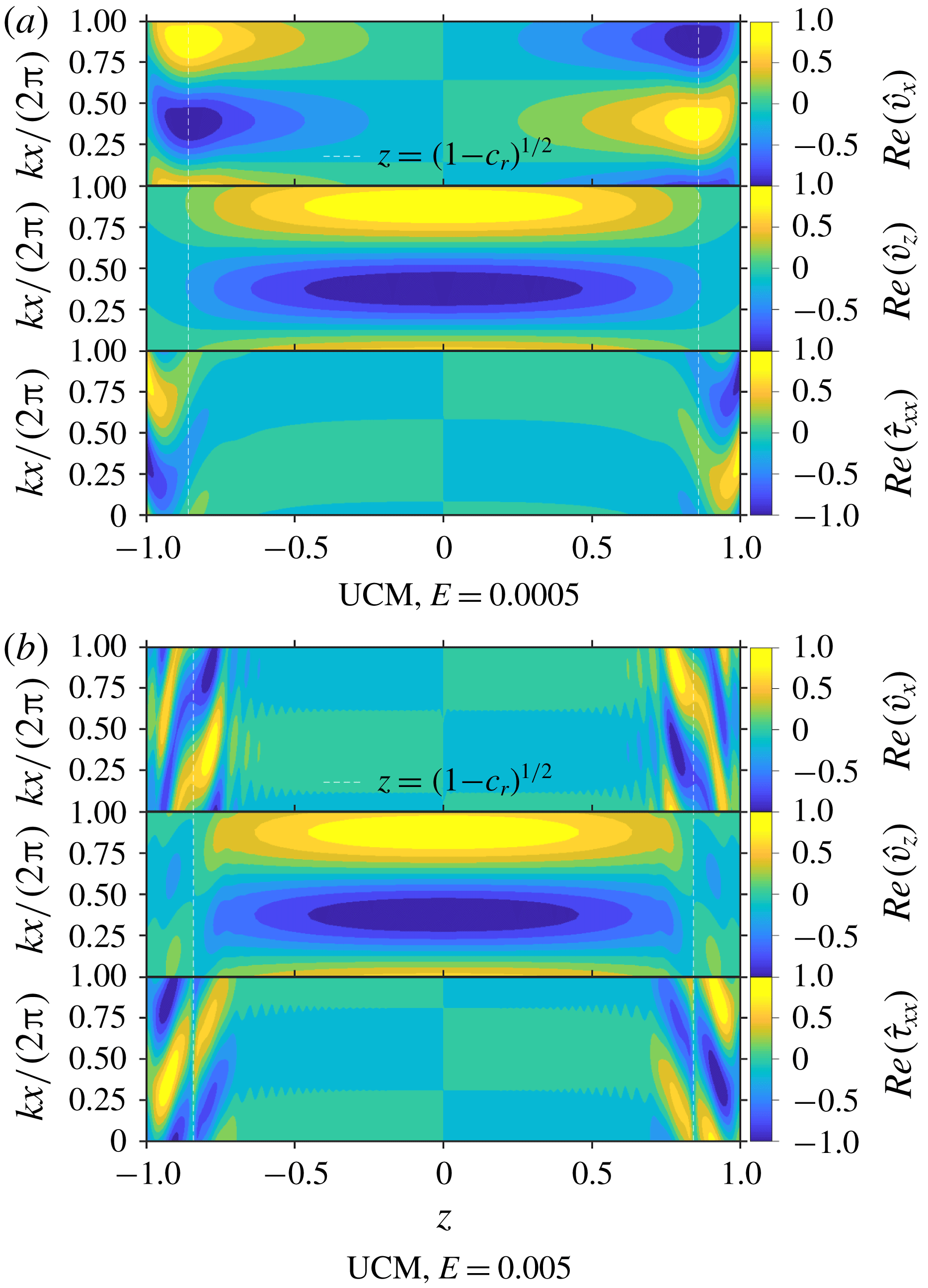
It is also useful to examine the structure of the unstable modes in the physical
 $x$
–
 $z$
plane, shown in figure 14, as this can be easily compared with results from DNS. To this end, we show the structure of
 $\hat{v}_{x}(x,z)$
,
 $\hat{v}_{z}(x,z)$
and
 $\hat{\unicode[STIX]{x1D70F}}_{xx}(x,z)$
. It must be noted that for a Newtonian fluid, the structures of
 $\hat{\unicode[STIX]{x1D70F}}_{xx}(x,z)$
and
 $\hat{v}_{x}(x,z)$
are identical, since the
 $xx$
-component of the stress is directly proportional to the perturbation
 $x$
-velocity. However, for a viscoelastic fluid, the elastic terms in the constitutive relation alter this picture. We show the structure of mode
 $A1(a)$
(figure 14
a), which is the elastically modified Newtonian (unstable) TS mode at
 $E=0.0005$
, and the structure of mode
 $A1(b)$
(figure 14
b) at
 $E=0.005$
, where the mode bifurcation had already occurred. The disturbance velocity
 $\hat{v}_{x}(x,z)$
is virtually identical to that of the Newtonian TS mode, and its structure indicates that it is largely confined near the wall, unlike
 $\hat{v}_{z}(x,z)$
, and the extent of confinement is sharper for
 $E=0.005$
compared to
 $E=0.0005$
. Interestingly, for both the modes,
 $\hat{\unicode[STIX]{x1D70F}}_{xx}(x,z)$
, while being confined near the walls, appears to go to zero near the location of the critical layer for
 $E=0.005$
. This is very different from the results of Shekar et al. (Reference Shekar, McMullen, Wang, McKeon and Graham2019) for a FENE-P fluid, wherein
 $\hat{\unicode[STIX]{x1D70F}}_{xx}$
exhibits a sharp maximum at the critical layer. We have verified that this difference in structure is primarily due to the difference in the solvent to polymer viscosity ratio (
 $\unicode[STIX]{x1D6FD}$
); indeed, with
 $\unicode[STIX]{x1D6FD}=0.97$
, similar to Shekar et al. (Reference Shekar, McMullen, Wang, McKeon and Graham2019), the eigenfunction for
 $\unicode[STIX]{x1D70F}_{xx}$
showed a very sharp localization for the parameters (
 $Re=6000$
, as opposed to
 $Re=1500$
used by Shekar et al. (Reference Shekar, McMullen, Wang, McKeon and Graham2019)) chosen in this study. This suggests that the mechanism of the elasto-inertial mode identified in this study is different from that proposed for the elastically modified TS mode of Shekar et al. (Reference Shekar, McMullen, Wang, McKeon and Graham2019).
In the following subsection, we discuss in detail how the elastically modified TS mode (labelled below as
 $A1(a)$
) transforms to the antisymmetric mode shown in figure 13(c) (labelled below as
 $A1(b)$
).
(a) Neutral stability curves for eigenmode
 $A1$
for
 $0\leqslant E\leqslant 0.0005$
. (b) Qualitative changes in these curves with increase in
 $E$
ranging
 $0.0005\leqslant E\leqslant 0.0018$
. (c) The curve for eigenmode
 $A1$
splits into two separate curves
 $A1(a)$
(lower and smaller lobe) and
 $A1(b)$
as
 $E$
is increased from
 $0.0018$
to
 $0.0022$
. (d) Evolution of the curves after splitting into two parts (
 $A1(a)$
(smaller loop) and
 $A1(b)$
) as
 $E$
is increased from
 $0.0022$
to
 $0.0035$
.

4.2.1 Effect of fluid elasticity on the Tollmien–Schlichting mode
We examine here the role of fluid elasticity on the neutral curve for the TS mode in the
 $Re$
–
 $k$
plane (the elastically modified TS-mode, referred to as mode
 $A1(a)$
hereafter). Figures 15(a) to 15(d) show the neutral stability curves obtained by tracing the loci of the points with
 $c_{i}=0$
that separate stable and unstable regions; the flow being unstable inside the neutral curves. The minimum Reynolds number on the neutral curve is the critical Reynolds number
 $Re_{c}$
and the corresponding wavenumber is the critical wavenumber
 $k_{c}$
, both being functions of
 $E$
; thus, for the Newtonian case,
 $E=0$
, one has
 $Re_{c}=5772.2$
with
 $k_{c}=1.02$
. To begin with, as
 $E$
increases, the neutral stability curve shifts towards lower Reynolds numbers and slightly higher wavenumbers and hence the flow becomes more unstable (figure 15
a). This is consistent with the trends first reported by Sureshkumar & Beris (Reference Sureshkumar and Beris1995b
), who, however, did not report the neutral curves shown in figure 15(a). For
 $E>0.0005$
, the neutral curve starts to develop a two-lobed structure (figure 15
b). Given the upper bound,
 $Re=10^{4}$
, that applies to the current study, we find that for
 $E\geqslant 0.0016$
, another unstable mode emerges which is not present in the Newtonian limit
 $E=0$
. This new unstable mode, labelled
 $A1(b)$
henceforth, appears only in a UCM fluid, and is therefore an elasto-inertial mode. The neutral curves corresponding to
 $A1(a)$
and
 $A1(b)$
for
 $E=0.0016$
(figure 15
b) show that for
 $Re>9543$
, the unstable modes
 $A1(a)$
and
 $A1(b)$
are distinct, in that, the variation of
 $c_{r}$
and
 $c_{i}$
for these modes exhibit two different curves. However, the two modes coalesce to form a single mode for
 $Re<9543$
(below the cusp-like region in figure 15
b) yielding a single unstable region. The
 $Re$
at which this modal coalescence between
 $A1(a)$
and
 $A1(b)$
occurs, as indicated by the cusp in the
 $Re-k$
plane, decreases as
 $E$
is further increased. Beyond
 $E=0.0019$
, the two-lobed structure develops a pair of distinct minima, and a second cusp appears for lower
 $Re$
(figure 15
c); however, only a single unstable mode is found until
 $E=0.0021$
. Thus, in the region below the upper cusp in the
 $Re-k$
plane, the two modes
 $A1(a)$
and
 $A1(b)$
become identical, and the two unstable regions fuse into one, yielding a single
 $c_{r}$
and
 $c_{i}$
versus
 $k$
curve. The
 $Re$
at which the lower cusp appears in the
 $Re-k$
plane increases with increase in
 $E$
, resulting in the upper and lower cusps approaching each other (figure 15
c). For
 $0.0021<E<0.0022$
(data not shown) the two cusps meet each other, leading to the neutral curve splitting into two separate ones for
 $E\gtrsim 0.0022$
as shown in figure 15(c), and concomitantly, the modes become separate once again.
Shrinking of the neutral stability curves and the formation of closed neutral stability ‘loops’ for eigenmode
 $A1(b)$
with increase in
 $E$
from
 $0.003$
to
 $0.008$
.

The aforementioned coalescence and bifurcation of the neutral curves was interpreted by Sureshkumar & Beris (Reference Sureshkumar and Beris1995b
) as two separate eigenfamilies in their study. The
 $x$
-velocity eigenfunction for the original TS instability, as already seen, is antisymmetric about the channel centreline (figure 13
a). The
 $x$
-velocity eigenfunctions that result, after the splitting of the original neutral curve, are therefore both antisymmetric (figure 13
c). The labelling of the two eigenfamilies (1 and 2 in the nomenclature of Sureshkumar & Beris (Reference Sureshkumar and Beris1995b
)) as
 $A1(a)$
and
 $A1(b)$
is justified because, as demonstrated above, for a range of
 $Re$
,
 $E$
and
 $k$
, the two eigenmodes become identical. In light of the above observation, the nomenclature used for labelling the modes in this section, and the new elasto-inertial modes examined in later sections, is as follows. The modes are numbered in increasing order of their critical Reynolds number, with the symmetry of the mode (about the centreline) being indicated by either an
 $A$
or an
 $S$
;
 $A$
here refers to antisymmetric and
 $S$
to symmetric modes. Thus, the alphabet
 $A$
in
 $A1$
refers to antisymmetry of the mode, and ‘1’ refers to the mode with the lowest critical Reynolds number (
 $Re_{c}$
).
Figure 15(d) shows that for
 $E\gtrsim 0.0024$
, the neutral curve for mode
 $A1(a)$
becomes a closed loop which, with a further increase in
 $E$
, shrinks in extent, while simultaneously moving towards higher
 $Re$
. It ceases to exist at
 $E>0.003$
. The neutral stability curve for the eigenmode
 $A1(b)$
shifts towards lower
 $Re$
as
 $E$
increases further, making it more unstable, with a lowest value of
 $Re_{c}=1210.9$
at
 $E=0.0066$
. From figure 16, it is clear that for
 $E=0.006,0.007$
and
 $0.008$
, the neutral curve for eigenmode
 $A1(b)$
also becomes a closed curve, which again shrinks, eventually ceasing to exist for
 $E>0.008$
.
Porteous & Denn (Reference Porteous and Denn1972) were among the first to analyse the stability of viscoelastic plane Poiseuille flow and reported neutral curves for different
 $E$
. We have confirmed that their neutral curves correspond to modes
 $A1(a),A1(b)$
(and the mode
 $A2$
discussed below) found in this study. In the results of Porteous & Denn (Reference Porteous and Denn1972), the neutral curve for eigenmode
 $A1(a)$
did not exist at
 $E=0.005$
, and the reason for this is clear from figures 15(c) and 15(d), which show that the neutral curve disappears for
 $E>0.003$
. This disappearance also explains the abrupt ending of the curve depicting the variation of
 $Re_{c}$
with
 $E$
for eigenfamily 1 in figure 4 of Sureshkumar & Beris (Reference Sureshkumar and Beris1995b
). These authors extended the results of Porteous & Denn (Reference Porteous and Denn1972) for the
 $A1(a)$
and
 $A1(b)$
modes and showed the existence of a minimum critical Reynolds number
 $Re_{c}$
for mode
 $A1(a)$
at
 $E\approx 0.0025$
. For mode
 $A1(b)$
, the data presented by Sureshkumar & Beris (Reference Sureshkumar and Beris1995b
) were limited to
 $E\leqslant 0.0035$
.
Neutral stability curves (a)
 $Re$
versus
 $k$
, and (b)
 $c_{r}$
versus
 $k$
, for
 $E=0.005$
. Points marked on panel (a) represent the
 $(k,Re)$
pairs for which the eigenspectra and eigenfunctions for the unstable modes are discussed further. The neutral curve for mode
 $A1(b)$
corresponds to the mode that splits from the continuation of the Newtonian TS mode to finite
 $E$
. At
 $E=0.005$
, the neutral curve of the original TS mode (mode
 $A1(a)$
in our nomenclature) does not exist. The neutral curves for modes
 $A2$
–
 $A4$
and
 $S1$
–
 $S3$
belong to the new elasto-inertial instabilities found in this study.

4.2.2 New elasto-inertial unstable eigenmodes
Within the parameter range
 $0<Re\leqslant 10^{4}$
and
 $0<E\leqslant 0.01$
, in addition to the modes
 $A1(a)$
and
 $A1(b)$
discussed above, we identified three new unstable antisymmetric (
 $A2$
–
 $A4$
) modes and three symmetric ones (
 $S1$
–
 $S3$
). A representative sample of
 $k$
and
 $Re$
values for
 $E=0.005$
, and the unstable modes that are found in this study, are mentioned in table 1. The neutral stability curves for all instabilities identified in this work are shown in figure 17(a) for
 $E=0.005$
. At
 $E=0.005$
, out of the seven eigenmodes tracked in this study, the eigenmode
 $A1(b)$
is the most unstable. Antisymmetric eigenmodes typically become unstable at a lower
 $Re_{c}$
in comparison to the symmetric modes.
Neutral stability curves (a)
 $Re$
versus
 $k$
, and (b)
 $c_{r}$
versus
 $k$
, for
 $E=0.0035$
.

Unstable eigenmodes found for various combinations of
 $k$
and
 $Re$
for a fixed value of the elasticity number
 $E=0.005$
.

In order to demonstrate the effect of decreasing
 $E$
, another set of neutral curves for
 $E=0.0035$
is shown in figure 18(a). It is evident that, as
 $E$
decreases, the neutral curves shift towards higher
 $Re$
, while also increasing in extent along the
 $k$
-axis. Thus, for
 $E=0.0035$
, the neutral curves for modes
 $S3$
and
 $A4$
have moved to
 $Re>10^{4}$
. Figures 17(b) and 18(b) show the corresponding variation of
 $c_{r}$
with
 $k$
along the neutral curves. One important feature that emerges from these figures is that the wave speeds of all unstable modes lie within the range of base-flow velocities
 $0\leqslant c_{r}\leqslant 1$
. For large
 $Re$
, the
 $c_{r}$
are relatively small (
 $c_{r}\lesssim 0.3$
) implying that the mechanism underlying the instability involves the confining walls in an essential way. This is discussed further in § 4.2.4.
Filtered eigenspectrum (a) for
 $E=0.005,k=1.6,Re=4000$
(location 1 in figure 17
a) for
 $N=500$
. Panel (b) shows the normalized
 $\tilde{v}_{x}$
eigenfunction corresponding to the unstable mode
 $0.3784+0.00552\text{i}$
shown in (a).

We now present a few representative eigenspectra and eigenfunctions, for the unstable modes, for the
 $(k,Re)$
combinations marked by circles within the different neutral curves in figure 17(a). The eigenspectrum for
 $E=0.005$
,
 $k=1.6$
and
 $Re=4000$
, corresponding to point 1 in figure 17(a), is shown in figure 19(a). Only one unstable mode is present for the said parameters, and this is the eigenmode
 $A2$
. The corresponding streamwise velocity (
 $\tilde{v}_{x}$
) eigenfunction appears in figure 19(b). The eigenspectrum for
 $E=0.005$
,
 $k=1.3$
and a higher
 $Re=8000$
(point 2 in figure 17
a) shows three unstable modes (figure 20
a). The corresponding eigenfunctions, in decreasing order of their growth rates, are shown in figures 20(b), 20(c) and 20(d). The leading mode is the eigenmode
 $A2$
, and the two other eigenvalues are the new unstable eigenmodes, namely
 $A3$
and
 $S2$
, identified here for the first time. The eigenspectrum for
 $E=0.005$
,
 $k=1.67$
and
 $Re=9800$
(corresponding to point 3 on figure 17
a) again shows three unstable modes (figure 21(a)). A higher value
 $N=900$
is required for an accurate resolution of these unstable modes owing to the finer-scaled structures in the corresponding eigenfunctions for this set of parameters. The most unstable eigenvalue belongs to the family
 $A3$
whereas the two other eigenvalues belong to new families
 $A4$
and
 $S3$
. The eigenfunctions for the three unstable eigenmodes of this eigenspectrum are shown in figures 21(b), 21(c) and 21(d).
(a) Filtered eigenspectrum for
 $E=0.005,k=1.3,Re=8000$
(location 2 in figure 17
a) for
 $N=500$
. Panels (b–d) show the normalized eigenfunctions for
 $\tilde{v}_{x}$
corresponding to the three unstable modes shown in panel (a).

Filtered eigenspectrum (a) for
 $E=0.005,k=1.67,Re=9800$
(location 3 in figure 17
a) for
 $N=900$
. Panels (b–d) show the normalized eigenfunctions for
 $\tilde{v}_{x}$
corresponding to the three unstable modes shown in (a).

Evolution of the unstable modes
 $A2$
and
 $A3$
from the
 $E\rightarrow 0$
limit: panel (a) shows the spectra (symbols) and results from the shooting procedure (continuous line) for the scaled growth rate
 $kWc_{i}$
versus
 $c_{r}$
for mode
 $A2$
. Panel (b) shows the Newtonian spectra (symbols) and shooting (continuous line) results for mode
 $A3$
at different
 $E$
. The inset in panel (b) zooms into the region where the mode becomes unstable.

4.2.3 Origin of the new elasto-inertial unstable modes
The neutral stability curves shown, for example, in figure 18, do not contain the information on whether the new unstable modes identified in this study are a continuation, to finite
 $E$
, of the stable modes in the spectrum for Newtonian channel flow, or whether they are genuinely new modes that do not have any counterparts in the Newtonian spectrum. If the latter scenario holds, then, the growth rates of the modes should diverge to
 $-\infty$
in the limit
 $E\rightarrow 0$
. In this case, it is still possible for the modes to emerge either from the continuous spectrum or the HFGL line, since both these features of the viscoelastic spectrum have
 $c_{i}\propto 1/E$
for
 $E\rightarrow 0$
. In order to understand this better, we continued the unstable modes
 $A2$
and
 $A3$
to small
 $E$
, and the results are shown in figure 22. The unstable mode
 $A2$
smoothly continues to an HFGL mode in the limit
 $E\rightarrow 0$
. In order to illustrate this better, in figure 22(a), we plot
 $kWc_{i}$
, since
 $c_{i}=-1/(2kW)$
for the HFGL modes, and the quantity
 $kWc_{i}=-0.5$
. The continuous line is the result from the shooting code, while the discrete symbols are results from the spectral method for a few representative values of
 $E$
. In figure 22(b), we show the evolution of the unstable mode
 $A3$
, which (in contrast to
 $A2$
) smoothly continuous (as
 $E\rightarrow 0$
) to the third mode in the
 $A$
-branch of the Newtonian spectrum. Our results for the other elasto-inertial modes (not shown in the figures) show that similar to
 $A2$
, the modes
 $A4$
,
 $S1$
and
 $S3$
continue to one of the HFGL modes as
 $E\rightarrow 0$
. However, the mode
 $S2$
, similar to
 $A3$
, smoothly continues to a stable mode in the Newtonian spectrum as
 $E\rightarrow 0$
. Thus, it appears that there is no generic trend with regard to the origin of the new elasto-inertial unstable modes in the Newtonian limit.
Based on the eigenfunctions presented here, all the new unstable modes are qualitatively similar in that the disturbances are confined close to the walls. The
 $c_{r}$
for these modes are small (
 $c_{r}<0.45$
) and the maximum oscillation amplitude and the reduced spatial frequency occurs in the vicinity of the critical layer, in a manner similar to the least stable modes of the hourglass structure seen earlier (figures 10
d and 13
c). This similarity with the least stable hourglass modes remains true for both the symmetric and antisymmetric modes. In all cases considered, the length scale of the oscillations decreases with increasing
 $Re$
. More unstable modes could well be present at higher
 $Re$
and
 $E$
, but on account of the spatial scales in the eigenfunctions (shown, for example, in figures 19
b, 20
b and 21
b) becoming increasingly small, computation of eigenvalues (via either of the two methods used) becomes difficult. It is necessary to either take closer initial guesses (for the shooting method) or consider a higher number of collocation points (for the spectral method).
Variation of neutral stability curves with
 $E$
for eigenmodes (a)
 $A2$
, and (b)
 $S1$
.

4.2.4 Neutral stability curves for higher unstable elasto-inertial modes
In this section, we examine the role of fluid elasticity on the neutral stability curves for the new elasto-inertial unstable modes (
 $A2$
–
 $A4$
and
 $S1$
–
 $S3$
) found in this study. A similar discussion for the elastically modified TS mode (
 $A1(a)$
) and the neutral curve that coalesced/bifurcated from
 $A1(a)$
, viz.,
 $A1(b)$
, was presented in § 4.2.1. Figure 23 shows that the neutral stability curves for both modes
 $A2$
and
 $S1$
shift to lower
 $Re$
as
 $E$
is increased. Similar behaviour is observed for modes
 $A3$
and
 $S2$
(not shown). For the values of
 $E$
explored, the neutral stability curves for modes
 $A1(a)$
,
 $A1(b)$
and
 $A2$
form closed loops at sufficiently high
 $E$
. We expect this trend to carry over to other higher modes as well at high enough
 $E$
, but could not explicitly verify this due to computational difficulties associated with accessing that regime.
Figure 24(a) shows the variation of
 $Re_{c}$
with
 $E$
for all the modes identified in this study. As indicated, our results compare well with the (limited) results reported in Sureshkumar & Beris (Reference Sureshkumar and Beris1995b
). For eigenmodes
 $A1(a)$
,
 $A1(b)$
and
 $A2$
the critical Reynolds number
 $Re_{c}$
first decreases with increasing
 $E$
, passing through a minimum, before increasing again. This feature could not be explored for the modes higher than
 $A2$
for the values of
 $E$
probed (
 $E\leqslant 0.01$
). All three eigenfamilies exist only over a finite range of
 $E$
, this arising from the shrinking and subsequent disappearance of the corresponding neutral loops, in the
 $Re$
–
 $k$
plane, at critical values of
 $E$
(as discussed earlier in § 4.2.1). For the modes
 $A1(a)$
and
 $A1(b)$
, the threshold values are
 $E\approx 0.003$
and
 $0.008$
, respectively. For the
 $A2$
mode, the threshold
 $E$
might lie just outside the range of
 $E$
(
 ${\leqslant}0.01$
) examined here. Our expectation that the neutral loop corresponding to mode
 $A2$
will nevertheless close up is reinforced by the appearance of the non-monotonicity in
 $Re_{c}$
(figure 24
a). This is because, for modes
 $A1(a)$
and
 $A1(b)$
, the non-monotonicity appears just before the values of
 $E$
for which the neutral loop begins to shrink in size. In general, the critical
 $Re$
for a given modal family initially decreases with
 $E$
, and after reaching a minimum, again increases with
 $E$
. The neutral curve of a given family reduces to a shrinking loop that disappears beyond a critical
 $E$
. Concomitantly, new (unstable) modal families continue to appear as
 $E$
is increased, albeit with larger values of
 $Re_{c}$
. Thus, if
 $Re$
is fixed, plane Poiseuille flow of a UCM fluid is eventually stable at sufficiently high
 $E$
.
Of the three eigenmodes above, the lowest
 $Re_{c}=1210.9$
(at
 $E=0.0066$
) occurs for
 $A1(b)$
. In cases where data are available, for
 $E\ll 1$
,
 $Re_{c}\propto E^{-1}$
for eigenmodes
 $S1$
and
 $S2$
, whereas
 $Re_{c}\propto E^{-5/4}$
for eigenmodes
 $A2$
and
 $A3$
. The phase speed
 $c_{r,c}\propto E^{1/2}$
for all the modes except
 $A1(a)$
(figure 24
b), thus indicating that the unstable elasto-inertial modes are a type of ‘wall modes’ wherein the disturbances are confined to a thin region near the wall (Schmid & Henningson Reference Schmid and Henningson2001). The critical wavenumber
 $k_{c}\propto E^{-1/2}$
for eigenmodes
 $S1$
and
 $S2$
, while it scales as
 $E^{-1/4}$
for eigenmode
 $A3$
as shown in figure 24(c). The data for mode
 $A2$
, for the lowest values of
 $E$
probed, are suggestive of the scaling
 $k_{c}\sim E^{-1/4}$
similar to
 $A3$
.
We also analysed the trend exhibited by the critical frequency corresponding to the minimum of the
 $Re$
–
 $k$
neutral curves for various modal families. When the critical frequency,
 $\unicode[STIX]{x1D714}_{c}^{\ast }$
, is made dimensionless using the relaxation time,
 $\unicode[STIX]{x1D706}$
, the resulting quantity can be interpreted as a Deborah number
 $De_{c}=\unicode[STIX]{x1D714}_{c}^{\ast }\unicode[STIX]{x1D706}=Wk_{c}c_{r,c}$
. When the values of
 $De_{c}$
for various modes are plotted against
 $E$
(figure 24
d), they seem to approach an
 $O(1)$
constant as
 $E\rightarrow 0$
, although the constants are different for different modes. Scaling arguments given below also imply that, for the class of wall modes,
 $De_{c}\sim O(1)$
for
 $E\ll 1$
.
Variation of critical parameters with
 $E$
for modes
 $A1(a),A1(b),A2,A3,S1$
and
 $S2$
for
 $E\leqslant 0.01$
: (a)
 $Re_{c}$
versus
 $E$
, eigenmodes
 $A2$
and
 $A3$
scale as
 $Re_{c}\propto E^{-5/4}$
, and eigenmodes
 $S1$
and
 $S2$
scale as
 $Re_{c}\propto E^{-1}$
, (b)
 $c_{r}$
versus
 $E$
, eigenmodes
 $A2,A3,S1$
and
 $S2$
scale as
 $c_{r}\propto E^{1/2}$
, (c)
 $k_{c}$
versus
 $E$
, eigenmodes
 $S1$
and
 $S2$
scale as
 $k_{c}\propto E^{-1/2}$
, and eigenmodes
 $A3$
and
 $A2$
at the lower
 $E$
end, scale as
 $k_{c}\propto E^{-1/4}$
. Present results are also compared with those of Sureshkumar & Beris (Reference Sureshkumar and Beris1995b
) (denoted as
 $SB1$
and
 $SB2$
). The insets in each panel show the variation for mode
 $A1(a)$
and its approach to the Newtonian TS mode as
 $E\rightarrow 0$
, and (d) the variation of the dimensionless critical frequency
 $De_{c}$
with
 $E$
for modes
 $A2$
,
 $A3$
,
 $S1$
and
 $S2$
shows that it approaches an
 $O(1)$
constant as
 $E\rightarrow 0$
.

The numerically obtained scalings for
 $Re$
,
 $c_{r}$
and
 $k$
in the limit
 $E\ll 1$
may be rationalized using a boundary layer analysis near the walls. It is worth emphasizing that this scaling analysis does not explain why the modes are unstable, but only serves to organize the elasto-inertial unstable modes identified in this study into a class of viscoelastic wall modes. In the limit
 $Re\gg 1$
and
 $E\ll 1$
, there is a thin ‘wall layer’ near the walls of (non-dimensional) thickness
 $\unicode[STIX]{x1D6FF}\ll 1$
. The scalings for
 $Re$
,
 $k$
,
 $\unicode[STIX]{x1D6FF}$
and
 $c_{r}$
in terms of
 $E$
can be derived by rescaling the (4.10)–(4.15) in the region near the wall as follows. The wall-normal coordinate
 $z$
near the wall at
 $z=1$
can be expressed as
 $z=1-\unicode[STIX]{x1D6FF}\unicode[STIX]{x1D709}$
. In the limit
 $Re\gg 1$
,
 $E\ll 1$
, the eigenvalue
 $c$
is asymptotically small, and hence we expand
 $c=\unicode[STIX]{x1D6FF}c^{(0)}$
. The derivatives near the wall get rescaled as
 $\text{d}/\text{d}z=-(1/\unicode[STIX]{x1D6FF})(\text{d}/\text{d}\unicode[STIX]{x1D709})\equiv -\unicode[STIX]{x1D6FF}^{-1}{\mathcal{D}}$
, where
 ${\mathcal{D}}\equiv \text{d}/\text{d}\unicode[STIX]{x1D709}$
. The base-flow profile becomes
 $U=1-z^{2}\equiv 2\unicode[STIX]{x1D6FF}\unicode[STIX]{x1D709}-\unicode[STIX]{x1D6FF}^{2}\unicode[STIX]{x1D709}^{2}$
, which for
 $\unicode[STIX]{x1D6FF}\ll 1$
implies that
 $U\sim \unicode[STIX]{x1D6FF}$
near the wall. Using the boundary layer rescaling, equations (3.8)–(3.13) are modified for the region near the wall as
 $$\begin{eqnarray}\displaystyle & \displaystyle -\frac{1}{\unicode[STIX]{x1D6FF}}{\mathcal{D}}\tilde{v}_{z}+\text{i}k\tilde{v}_{x}=0, & \displaystyle\end{eqnarray}$$
 $$\begin{eqnarray}\displaystyle & \displaystyle Re\{\text{i}k(2\unicode[STIX]{x1D6FF}\unicode[STIX]{x1D709}-\unicode[STIX]{x1D6FF}^{2}\unicode[STIX]{x1D709}^{2}-\unicode[STIX]{x1D6FF}c^{(0)})\tilde{v}_{x}-2(1-\unicode[STIX]{x1D6FF}\unicode[STIX]{x1D709})\tilde{v}_{z}\}=-\text{i}k\tilde{p}+\text{i}k\tilde{\unicode[STIX]{x1D70F}}_{xx}-\unicode[STIX]{x1D6FF}^{-1}{\mathcal{D}}\tilde{\unicode[STIX]{x1D70F}}_{xz}, & \displaystyle\end{eqnarray}$$
 $$\begin{eqnarray}\displaystyle & \displaystyle Re\text{i}k(2\unicode[STIX]{x1D6FF}\unicode[STIX]{x1D709}-\unicode[STIX]{x1D6FF}^{2}\unicode[STIX]{x1D709}^{2}-\unicode[STIX]{x1D6FF}c^{(0)})\tilde{v}_{z}=-\unicode[STIX]{x1D6FF}^{-1}{\mathcal{D}}\tilde{p}+\text{i}k\tilde{\unicode[STIX]{x1D70F}}_{xz}-\unicode[STIX]{x1D6FF}^{-1}{\mathcal{D}}\tilde{\unicode[STIX]{x1D70F}}_{zz}, & \displaystyle\end{eqnarray}$$
 $$\begin{eqnarray}\displaystyle & & \displaystyle \{1+\text{i}kW(2\unicode[STIX]{x1D6FF}\unicode[STIX]{x1D709}-\unicode[STIX]{x1D6FF}^{2}\unicode[STIX]{x1D709}^{2}-\unicode[STIX]{x1D6FF}c^{(0)})\}\tilde{\unicode[STIX]{x1D70F}}_{xx}=\left[\left\{4W(1-\unicode[STIX]{x1D6FF}\unicode[STIX]{x1D709})\unicode[STIX]{x1D6FF}^{-1}{\mathcal{D}}+2\text{i}k\right.\right.\nonumber\\ \displaystyle & & \displaystyle \quad \left.\left.+\,16\text{i}kW^{2}(1-\unicode[STIX]{x1D6FF}\unicode[STIX]{x1D709})^{2}\right\}\tilde{v}_{x}-16W^{2}(1-\unicode[STIX]{x1D6FF}\unicode[STIX]{x1D709})\tilde{v}_{z}\right]-4W(1-\unicode[STIX]{x1D6FF}\unicode[STIX]{x1D709})\tilde{\unicode[STIX]{x1D70F}}_{xz},\end{eqnarray}$$
 $$\begin{eqnarray}\displaystyle & & \displaystyle \{1+\text{i}kW(2\unicode[STIX]{x1D6FF}\unicode[STIX]{x1D709}-\unicode[STIX]{x1D6FF}^{2}\unicode[STIX]{x1D709}^{2}-\unicode[STIX]{x1D6FF}c^{(0)})\}\tilde{\unicode[STIX]{x1D70F}}_{xz}=\left[-\unicode[STIX]{x1D6FF}^{-1}{\mathcal{D}}\tilde{v}_{x}+\left\{\text{i}k\right.\right.\nonumber\\ \displaystyle & & \displaystyle \quad \left.\left.+\,8\text{i}kW^{2}(1-\unicode[STIX]{x1D6FF}\unicode[STIX]{x1D709})^{2}+2W\right\}\tilde{v}_{z}\right]-2W(1-\unicode[STIX]{x1D6FF}\unicode[STIX]{x1D709})\tilde{\unicode[STIX]{x1D70F}}_{zz},\end{eqnarray}$$
 $$\begin{eqnarray}\displaystyle \{1+\text{i}kW(2\unicode[STIX]{x1D6FF}\unicode[STIX]{x1D709}-\unicode[STIX]{x1D6FF}^{2}\unicode[STIX]{x1D709}^{2}-\unicode[STIX]{x1D6FF}c^{(0)})\}\tilde{\unicode[STIX]{x1D70F}}_{zz}=-2\{\unicode[STIX]{x1D6FF}^{-1}{\mathcal{D}}+2\text{i}kW(1-\unicode[STIX]{x1D6FF}\unicode[STIX]{x1D709})\}\tilde{v}_{z}. & & \displaystyle\end{eqnarray}$$
Near the walls,
 $(U-c)\sim \unicode[STIX]{x1D6FF}$
. For
 $E\ll 1$
, our numerical results show that
 $k_{c}$
becomes large (figure 24
c), and so we set
 $k\sim \unicode[STIX]{x1D6FF}^{-1}$
in the following analysis. The left side of the linearized constitutive equations reveal that in order for the elastic stresses and viscous relaxation to be of the same order, we require
 $W\sim O(1)$
, or
 $Re\sim E^{-1}$
. Further, the linearized constitutive relations indicate that
 $\tilde{\unicode[STIX]{x1D70F}}_{zz}\sim \tilde{\unicode[STIX]{x1D70F}}_{xz}\sim \tilde{\unicode[STIX]{x1D70F}}_{xx}\sim \unicode[STIX]{x1D6FF}^{-1}$
. The linearized
 $x$
-momentum equation indicates that
 $Re\sim \unicode[STIX]{x1D6FF}^{-1}\unicode[STIX]{x1D70F}_{xz}$
, which then yields
 $Re\sim \unicode[STIX]{x1D6FF}^{-2}$
. Using
 $Re\sim E^{-1}$
we therefore obtain the following scaling relationships in terms of
 $E$
for
 $E\ll 1$
:
 $$\begin{eqnarray}\displaystyle \unicode[STIX]{x1D6FF}\sim E^{1/2},\quad k\sim E^{-1/2},\quad Re\sim E^{-1},\quad c_{r}\sim E^{1/2}. & & \displaystyle\end{eqnarray}$$
From figures 24(a) and 24(c) it is clear that the modes
 $S1$
and
 $S2$
follow the above scaling very well. The scalings are not followed exactly for the antisymmetric modes in the range of
 $E$
explored. It is possible that the numerical and asymptotic scaling exponents will agree for much lower values of
 $E$
and higher values of
 $Re$
, a regime that is difficult to access numerically.
5 Conclusions
We have carried out a comprehensive linear stability analysis for plane Poiseuille and Couette flows of a UCM fluid using a judicious combination of pseudo-spectral and shooting methods. While the spectral code was used for an extensive search of the
 $Re$
–
 $E$
parameter space, with an objective to detect new unstable modes, the shooting method was used to track the neutral stability envelopes in the
 $Re$
–
 $k$
plane. The main conclusion from the present study is that multiple unstable modes, both symmetric and antisymmetric, exist for viscoelastic plane Poiseuille flow. The origin of the instabilities may be attributed to the competing effects of elasticity and inertia. The identified unstable modes appear to be part of an infinite hierarchy of elasto-inertial instabilities. For Newtonian channel flow, the unstable TS mode is an antisymmetric mode; hitherto, previous studies on viscoelastic channel flows have also found only antisymmetric unstable modes. Our findings concerning symmetric unstable modes in viscoelastic channel flow mark a major departure from this picture.
We found seven unstable eigenmodes in the range of
 $Re=[0,10^{4}]$
, out of which three (
 $S1$
–
 $S3$
) are symmetric and four (
 $A1$
–
 $A4$
) are antisymmetric modes. The neutral curves for the eigenmodes
 $A1(a)$
and
 $A1(b)$
were found to fuse into a single unstable region over a range of
 $Re$
and
 $k$
for
 $E\leqslant 0.0021$
, while they split into two separate neutral curves for
 $E\geqslant 0.0022$
. Thus, we find both coalescence and subsequent bifurcation of eigenvalues corresponding to the aforementioned modes as
 $E$
is increased. The neutral curves in the
 $Re$
–
 $k$
plane form closed loops at sufficiently high
 $E$
, and the unstable region within these loops shrinks with increase in
 $E$
, with both modes
 $A1(a)$
and
 $A1(b)$
ceasing to exist for
 $E>0.003$
and
 $E>0.008$
, respectively. In the region of the parameter space probed, the eigenmode
 $A1(b)$
is found to be the most unstable, with the lowest critical Reynolds number
 $Re_{c}=1210.9$
for
 $E=0.0066$
with
 $k_{c}=1.615$
. Scalings for the critical parameters with the elasticity number
 $E$
were obtained in the limit of small
 $E$
(
 ${<}0.005$
), for
 $A2$
and higher modes. All unstable modes have the character of ‘wall modes’ in the limit
 $E\ll 1$
, with the phase speed being O(
 $E^{1/2}$
) for small
 $E$
.
It is pertinent here to discuss the role of solvent viscosity, characterized by the parameter
 $\unicode[STIX]{x1D6FD}$
(the ratio of solvent to solution viscosity, which is identically zero in a UCM fluid) on the new elasto-inertial modes identified in this study. Sureshkumar & Beris (Reference Sureshkumar and Beris1995b
) showed that solvent viscosity has a stabilizing effect on the continuation of the TS mode to finite
 $E$
. Preliminary results from our computations for an Oldroyd-B fluid also reveal that solvent viscous effects have a stabilizing role on the new elasto-inertial modes. Inclusion of solvent effects will also mitigate the amplitude of the rapid oscillations exhibited by some of the eigenfunctions. Similarly, the role of finite extensibility (characterized by the parameter
 $L$
denoting maximum chain extension, for example, in the FENE-P model) on the new elasto-inertial modes was found to be marginally stabilizing. While the stability boundaries in the
 $Re_{c}$
–
 $\unicode[STIX]{x1D6FD}$
and
 $Re_{c}$
–
 $L$
parameter space will be discussed in detail in a subsequent study (Authors’ paper in preparation: Role of solvent viscous effects and finite extensibility on elasto-inertial wall modes in viscoelastic channel flow.), it is nevertheless useful to assess the role of finite extension of the polymer on the oscillatory nature of the eigenfunctions of the elasto-inertial modes. These modes are characterized by high frequencies (denoted by
 $\unicode[STIX]{x1D714}$
), such that the Deborah number
 $De=\unicode[STIX]{x1D714}\unicode[STIX]{x1D706}$
for these modes is quite high
 ${\sim}10$
(figure 24
d), and hence the polymer does not stretch out much in response to the perturbation velocity gradient in a time of order
 $\unicode[STIX]{x1D714}^{-1}$
. Thus, finite extension effects cannot be expected to remove the oscillatory nature of the eigenfunctions. Inclusion of finite extension (as in the FENE-P model) also implies the onset of shear thinning, which leads to a modified base-state velocity profile. This effect is significant only for modest values of the ratio of the fully extended length to equilibrium coil size, and therefore cannot qualitatively alter the nature of the eigenfunctions for high molecular weight polymers.
It is useful to examine the relevance of these new modes of instability in a UCM fluid, which attempts to model a pure polymeric liquid (without any solvent), in practical situations. Typical viscosities in processes involving polymer melts are very high and the values of
 $Re$
are typically low. Therefore, the present results cannot directly be applied to such low
 $Re$
flows. Nevertheless, the UCM model is one of the simplest constitutive equations allowing for elastic effects, and hence it is important to have a comprehensive picture of its stability characteristics in canonical shear flows. This understanding might then help in the interpretation of stability characteristics of more involved nonlinear constitutive equations, thereby assisting in a general understanding of onset of transition in viscoelastic shear flows. Although it is difficult to make a direct comparison of the present results with experimental observations in the literature, the present work demonstrates that there exist instabilities which are driven by elastic effects even in viscoelastic plane shear flows. Prior studies have shown that, in the absence of inertia, viscoelastic plane shear flows are stable, and that curvature of the streamlines, and the associated hoop stresses, are essential (Shaqfeh Reference Shaqfeh1996) to initiate elasticity-driven instabilities in the non-inertial limit.
In stark contrast, the present study shows that upon inclusion of inertial effects, streamline curvature is not essential for elastically driven instabilities. In particular, it is possible that new elasto-inertial unstable modes (similar to the ones uncovered here) could be present even in flows with curved streamlines (Joo & Shaqfeh Reference Joo and Shaqfeh1992; Muller Reference Muller2008), which are not driven by the same mechanism that underlies the purely elastic instability in the absence of inertia. Considering the localized nature of the unstable mode near the walls (for small
 $E$
), it is also natural to speculate that a similar wall mode instability may well be present in viscoelastic pipe flows. There is indeed a precedent for finding a common mechanism underlying instabilities in channel and pipe flows: the recently discovered (Garg et al.
Reference Garg, Chaudhary, Khalid, Shankar and Subramanian2018) centre-mode instability (localized near the centreline of the pipe or channel) for an Oldroyd-B fluid was demonstrated to exist for both pressure-driven channel and pipe flows, although this instability does not persist in the limit of a UCM fluid. It remains to be seen whether a mechanism similar to the wall mode instability predicted for channel flows also applies to pipe flow of a UCM fluid.
Acknowledgements
The authors thank M. Khalid for instructive discussions regarding the FENE-P model.
Appendix A. Numerical methods and their validation
A.1 Numerical methods
The fluid governing equations and the stress equations along with the boundary conditions are discretized using the pseudospectral method involving interpolating polynomials. These interpolating polynomials in turn are constructed by using Chebyshev polynomials as orthogonal basis. The collocation points that we considered are the Chebyshev points of the second kind, or equivalently, the extrema on the domain
 $[-1,1]$
of the Chebyshev polynomial of degree
 $N-1$
, viz.,
 $T_{N-1}(z)$
, plus the two end points of the domain. This choice for the collocation points is known as the Gauss–Lobatto grid. The interpolating polynomial is constructed using cardinal functions (Canuto et al.
Reference Canuto, Hussaini, Quarteroni and Zang1988). Equations (3.8)–(3.14) are discretized using the pseudo-spectral method and the resulting equations can be formulated as a generalized matrix eigenvalue problem for the complex wave speed
 $c$
. The eigenvalue problem is solved using Matlab and the spurious eigenvalues are filtered by comparing the eigenspectrum obtained for two different grid sizes and rejecting the non-convergent (as decided by a pre-set tolerance) eigenvalues among the obtained sets. This method is a simple way to get rid of spurious eigenvalues (Schmid & Henningson Reference Schmid and Henningson2001). The physically genuine eigenvalues are independent of
 $N$
if
 $N$
is sufficiently high enough to resolve the smallest scales corresponding to a given eigenmode. In order to eliminate physically spurious eigenvalues, first the eigenspectrum is computed for two different values of
 $N$
. The eigenvalues from the two sets are compared based on a specified tolerance (for e.g.
 $10^{-4}$
, for agreement up to four significant digits) for the normalized difference between the eigenvalues obtained for two different
 $N$
. The eigenvalues which pass through the filtering step are treated as physically genuine eigenvalues, and the rest are either physically spurious or genuine eigenvalues that are not captured accurately at this chosen resolution.
In the shooting method, we numerically construct two linearly independent solutions for
 $\tilde{v}_{z}$
to (3.8)–(3.13) consistent with the boundary conditions at
 $z=-1$
. We integrate the governing equations using a fourth-order Runge–Kutta integrator with adaptive step-size control. At each step of integration we orthonormalize the two linearly independent solutions with Gram–Schmidt orthonormalization procedure so that the orthonormality of the computed solutions is maintained throughout the domain. After marching up to the other boundary at
 $z=1$
, the two linearly independent solutions are substituted into the boundary conditions at
 $z=1$
and a
 $2\times 2$
characteristic matrix is obtained. The determinant of this matrix is set to zero for the existence of non-trivial coefficients for the independent solutions. Starting with initial guesses obtained from eigenspectrum, we apply the Newton–Raphson iterative method to obtain convergence of the eigenvalue
 $c$
.
A.2 Validation of numerical schemes
Table 2 shows the comparison of results obtained from both the present spectral and shooting codes with those of Renardy & Renardy (Reference Renardy and Renardy1986) for plane Couette flow of UCM fluid. The number of the eigenvalues obtained in the eigenspectrum depends on the number of collocation points considered, therefore the number of eigenvalues obtained in the present analysis is larger than that of the results of Renardy & Renardy (Reference Renardy and Renardy1986). For comparison, we present only those eigenvalues in table 2 which correspond to the eigenvalues reported in Renardy & Renardy (Reference Renardy and Renardy1986). The results obtained in our study are in good agreement with those of Renardy & Renardy (Reference Renardy and Renardy1986). The present spectral and shooting results are more accurate and are in excellent agreement with each other.
Validation of numerical method: comparison of the present results with that of Renardy & Renardy (Reference Renardy and Renardy1986) for UCM plane Couette flow in a rigid channel for
 $W=0.2$
and
 $W=2.$

In table 3, we compare the present results for plane Poiseuille flow of UCM fluid with those of Sureshkumar & Beris (Reference Sureshkumar and Beris1995b
). According to Sureshkumar & Beris (Reference Sureshkumar and Beris1995b
), these eigenvalues are obtained at the critical values of Reynolds number and hence they reported the frequency
 $\unicode[STIX]{x1D714}\equiv kc$
to be purely real. We solved for the same set of parameters with both spectral and shooting methods and found that the growth rates are not identically zero, but have a very small magnitude. Therefore the frequencies that we have reported in this table are not purely real but complex. On comparison at lower values of elasticity number, we find that the phase speeds
 $c_{r}$
in the present results match up to two decimal places with those in case of Sureshkumar & Beris (Reference Sureshkumar and Beris1995b
), whereas the agreement between present spectral and shooting results is excellent. At higher values of elasticity number, the present results do not match well with that of Sureshkumar & Beris (Reference Sureshkumar and Beris1995b
) but the agreement between present spectrum and shooting results is excellent (up to at least five places after the decimal). The reason for these minor mismatches could perhaps be attributed to the different grid sizes considered in present case and in that of Sureshkumar & Beris (Reference Sureshkumar and Beris1995b
) while solving the eigenvalue problem.
Validation of numerical method: comparison of the present results with those of Sureshkumar & Beris (Reference Sureshkumar and Beris1995b ) for plane Poiseuille flow of UCM fluid in a rigid channel.

Table 4 shows the comparison of eigenvalues obtained from our numerical method with those of Lee & Finlayson (Reference Lee and Finlayson1986) for plane Poiseuille flow of Newtonian and UCM fluids at various
 $Re$
,
 $W$
and
 $k$
. To capture the eigenvalues at higher values of Weissenberg number using spectral method requires larger grid size. The results obtained by our numerical method are in good agreement with those reported in Lee & Finlayson (Reference Lee and Finlayson1986) and the results obtained by present spectral and shooting methods also match very well.
Validation of numerical method: comparison of the present results with those of Lee & Finlayson (Reference Lee and Finlayson1986) for plane Poiseuille flow of UCM fluid in a rigid channel.