1. Introduction
Turbulence is characterised by velocity fluctuations whose statistics are strongly scale-dependent. Probability density functions (p.d.f.s) of the velocity increments are approximately Gaussian at separation distances commensurate to and larger than the integral length scale, but display heavier tails as the separation length scale decreases through the inertial range and into the dissipative range of scales. This phenomenon, known as intermittency, presents a major challenge to creating accurate turbulence models. Over the years, a number of techniques have been developed to model intermittency, such as multifractals and superstatistics, which are reviewed in the following.
In the language of multifractal theory, multiscale observables can be written as a statistical mixture of a continuum of Hölder exponents. Each exponent
 $h$
occupies a set of dimension
 $D(h)$
and this determines the contribution of each
 $h$
to the full statistics (Mandelbrot Reference Mandelbrot1977; Parisi & Frisch Reference Parisi and Frisch1985; Falconer Reference Falconer1990; Meneveau & Sreenivasan Reference Meneveau and Sreenivasan1991). Among the observables to which multifractal theory has been successfully applied are velocity gradients (Nelkin Reference Nelkin1990; Chevillard & Meneveau Reference Chevillard and Meneveau2006; Ishihara, Gotoh & Kaneda Reference Ishihara, Gotoh and Kaneda2009; Johnson & Meneveau Reference Johnson and Meneveau2017; Pereira et al. Reference Pereira, Eça, Vaz and Girimaji2018; Luo, Shi & Meneveau Reference Luo, Shi and Meneveau2022), Eulerian velocity increments (Benzi et al. Reference Benzi, Paladin, Parisi and Vulpiani1984; Meneveau & Sreenivasan Reference Meneveau and Sreenivasan1991), Lagrangian velocity increments (Biferale et al. Reference Biferale, Boffetta, Celani, Devenish, Lanotte and Toschi2004; Chevillard et al. Reference Chevillard, Roux, Lévêque, Mordant, Pinton and Arnéodo2005, Reference Chevillard, Castaing, Arneodo, Lévêque, Pinton and Roux2012; Arnèodo et al. Reference Arnèodo2008) and Lagrangian acceleration (Biferale et al. Reference Biferale, Boffetta, Celani, Devenish, Lanotte and Toschi2004). Crucially, it provides a connection between the asymptotic scaling of all of these observables in terms of a single
 $D(h)$
function.
At first glance, superstatistics (Beck & Cohen Reference Beck and Cohen2003; Beck Reference Beck2004, Reference Beck2011) represents a complementary approach to model intermittency based on a mixture distribution. Applied to non-equilibrium statistical mechanics, superstatistics describes a mixture of Boltzmann statistics with the temperature as the mixing parameter (Beck & Cohen Reference Beck and Cohen2003; Beck Reference Beck2004, Reference Beck2011). In the context of turbulence, the mixing parameter may be, for instance, the energy dissipation. This description has been shown to capture non-Gaussian turbulence statistics both in the Eulerian (Beck Reference Beck2000) and Lagrangian frames (Reynolds Reference Reynolds2003; Beck Reference Beck2003, Reference Beck2007; Reynolds et al. Reference Reynolds, Mordant, Crawford and Bodenschatz2005). It is also worth noting that the multifractal model can be formulated in a way akin to superstatistics. Specifically, Chevillard et al. (Reference Chevillard, Castaing, Arneodo, Lévêque, Pinton and Roux2012) considered a superposition of Gaussian increment statistics with a fluctuating variance as a function of the Hölder exponents. Early approaches include those of Castaing, Gagne & Hopfinger (Reference Castaing, Gagne and Hopfinger1990), who produced K62 increment statistics as a superposition of Gaussian distributions with a fluctuating variance as a function of the dissipation rate, and Benzi et al. (Reference Benzi, Biferale, Paladin, Vulpiani and Vergassola1991), who generated velocity increment and gradient p.d.f.s with anomalous scaling from superpositions based on the random beta model. This indicates that intimate relations between the two approaches exist.
Previous applications of the multifractal and superstatistical approaches have focused on the modelling of individual random variables, e.g. two-point statistics. While the multifractal language provides a connection between the universal properties of different observables (Benzi et al. Reference Benzi, Biferale, Paladin, Vulpiani and Vergassola1991, Reference Benzi, Biferale and Toschi1998; Chevillard et al. Reference Chevillard, Castaing, Arneodo, Lévêque, Pinton and Roux2012), the interest in extending these approaches to modelling the statistics of entire random fields remains. Wilczek (Reference Wilczek2016) showed that a superposition of Gaussian characteristic functionals (i.e. a statistical ensemble of Gaussian fields) with a fluctuating correlation function is capable of producing non-Gaussianity and intermittency. This naturally leads to the question whether a mixture model with realistic multifractal properties comprising entire field statistics can be developed. A first step into this direction was recently taken by Friedrich et al. (Reference Friedrich, Peinke, Pumir and Grauer2021), who developed a model for field statistics with classic K62 multifractal scaling (Kolmogorov Reference Kolmogorov1962; Obukhov Reference Obukhov1962). The approach has been extended to enable a statistical refinement of sparse data sets by Lübke et al. (Reference Lübke, Friedrich and Grauer2023) and has furthermore been applied to the stochastic modelling of turbulent wind fields (Friedrich et al. Reference Friedrich, Moreno, Sinhuber, Wächter and Peinke2022). We mention as well a complementary approach to field statistics, where realisations of a random field are generated with properties compatible with multifractal theory. This can be done with the Gaussian multiplicative chaos, in a static (Chevillard et al. Reference Chevillard, Garban, Rhodes and Vargas2019) or dynamic approach (Apolinário et al. Reference Apolinário, Chevillard and Mourrat2022; Beck et al. Reference Beck, Bréhier, Chevillard, Grande and Ruffenach2024), as well as with multiplicative wavelet decompositions (Benzi, Biferale & Parisi Reference Benzi, Biferale and Parisi1993; Arnéodo, Bacry & Muzy Reference Arnéodo, Bacry and Muzy1998) or products of time series (Biferale et al. Reference Biferale, Boffetta, Celani, Crisanti and Vulpiani1998).
In this paper, we establish a relation between existing multifractal models and the superstatistical Gaussian field ensemble approach. We construct an ensemble of Gaussian fields that features increment and gradient statistics complying with a given multifractal singularity spectrum, albeit only for its even moments. This extends previous models based on Gaussian superpositions of two-point velocity increment p.d.f.s to field statistics that contains arbitrary multi-point p.d.f.s via superpositions of Gaussian characteristic functionals. From a conceptual point of view, this highlights close connections between the discussed previous approaches and lays the foundation for a future connection to statistical field theories based on the Navier–Stokes equation such as the functional approach (Hopf Reference Hopf1952; Ohkitani Reference Ohkitani2020).
The content is arranged as follows. In § 2, we review the multifractal modelling of Chevillard et al. (Reference Chevillard, Castaing, Arneodo, Lévêque, Pinton and Roux2012) and the ensemble of Gaussian fields of Wilczek (Reference Wilczek2016). In § 3, we show how the multifractal description can be generalised to a superstatistical characteristic functional. Section 4 demonstrates the approach with a simple example – the classic log-normal model. In § 5, a more general model is considered, with an arbitrary singularity spectrum, and realistic large-scale and viscous-range behaviour. Conclusions are drawn in § 6.
2. Theoretical background
2.1. Gaussian mixtures for multifractal velocity increment p.d.f.s
In this section, we summarise the formulation of multifractals as Gaussian mixtures put forward by Chevillard et al. (Reference Chevillard, Castaing, Arneodo, Lévêque, Pinton and Roux2012). The paper considers velocity increments
 $v = \delta _\ell u$
across a scale
 $\ell$
in the inertial range, i.e.
 $\eta \ll \ell \ll L$
, where
 $\eta$
denotes the Kolmogorov scale and
 $L$
the integral scale of the flow. The velocity increment, conditional on a given Hölder exponent
 $h$
, is modelled as a zero-mean Gaussian random variable, with p.d.f.
 \begin{equation} g( v;S(\ell ;h) ) = \frac {1}{\sqrt {2 \pi\! S(\ell ;h)}} \exp\! \left [ -\frac {v^2}{2 S(\ell ;h)} \right ] \! . \end{equation}
Notice that we have adopted a notation for the Gaussian p.d.f.
 $g(x; \sigma ^2)$
, where
 $\sigma ^2$
is the variance. Here,
 $S(\ell ;h)$
is the second-order structure function conditional on a given Hölder exponent, and behaves as
 \begin{equation} S(\ell ;h) = 2 \sigma _u^2 \left ( 1 + \left (\frac {L}{\ell }\right )^2\right )^{-h} \end{equation}
in the inertial and large-scale ranges. Compared with Chevillard et al. (Reference Chevillard, Castaing, Arneodo, Lévêque, Pinton and Roux2012), we have added a large-scale saturation. The large-scale root mean square velocity is denoted by
 $\sigma _u$
and
 $S(\ell ,h)$
correctly asymptotes to
 $2 \sigma _u^2$
as
 $\ell \to \infty$
. Moreover, this function shows an
 $(\ell /L)^{2h}$
scaling in the inertial range. In this framework, the p.d.f. of velocity increments is given by
 \begin{equation} f_v(v ; \ell ) = \int {\mathrm{d}} h \, f_{h}(h;\ell ) \, g(v;S(\ell ;h)), \end{equation}
where
 $f_{h}(h;\ell )$
is the probability density of Hölder exponents at fixed scale
 $\ell$
. This mixture of Gaussian random variables with fluctuating variance naturally gives rise to non-Gaussian statistics.
In this one-dimensional setting, the mixture distribution
 $f_h(h;\ell )$
provided by multifractal phenomenology, including the inertial and large-scale ranges, is given by
 \begin{equation} f_h(h; \ell ) = \begin{cases} \frac {1}{Z(\ell )} \left ( 1+ (L/\ell )^2 \right )^{-(1-D(h))/2}&\text{if }h_{\textit{min}} \leqslant h \leqslant h_{\textit{max}}, \\[3pt] 0 &\text{otherwise,}\end{cases} \end{equation}
where
 $D(h)$
is the multifractal singularity spectrum,
 $h_{\textit{min}}$
and
 $h_{\textit{max}}$
are bounds on the Hölder exponent (explained later), and
 $Z(\ell )$
is the normalisation of the p.d.f. A key assumption of the multifractal model, relevant for the subsequent discussion, is that
 $D(h)$
is assumed to be independent of
 $\ell$
over the inertial range of scales.
With this formulation, the velocity increment displays multifractal scaling exponents, at least for its even moments,
 \begin{equation} \langle v^n \rangle \sim \ell ^{\zeta _n}, \quad \text{where } \quad \zeta _n = \min _h \left [ nh + 1 - D(h) \right ]\! , \end{equation}
as can be shown with a steepest descent approximation in the limit of vanishing scale separation (Chevillard et al. Reference Chevillard, Castaing, Arneodo, Lévêque, Pinton and Roux2012). Due to the use of Gaussians, all odd-order moments of the velocity increments are zero. We remark, however, that Chevillard et al. (Reference Chevillard, Castaing, Arneodo, Lévêque, Pinton and Roux2012) address the skewness of the velocity increments by modifying the Gaussian base distribution.
There are several empirical models for
 $D(h)$
in the turbulence literature and, in § 3, we consider a change of variables where
 $D(h)$
can be freely specified. As explicit examples, we consider three representative models of singularity spectra: the log-normal, with a quadratic spectrum
 \begin{equation} D(h) = 1 - \frac {(h-h_0)^2}{2 \sigma _h^2}; \end{equation}
the She–Lévêque model (She & Lévêque Reference She and Lévêque1994), with spectrum
 \begin{equation} D(h) = -1 + 3\left [ \frac {1+\log \log \left (\frac {3}{2}\right )}{\log \left (\frac {3}{2}\right )} - 1 \right ]\left (h - \frac {1}{9}\right ) - \frac {3}{\log \left (\frac {3}{2}\right )}\left (h - \frac {1}{9}\right )\log \left (h-\frac {1}{9}\right )\!; \end{equation}
and the Sreenivasan–Yakhot model (Sreenivasan & Yakhot Reference Sreenivasan and Yakhot2021), defined by
 \begin{equation} D(h) = 1 - c - \beta h + 2 \sqrt {c \beta h}. \end{equation}
The free parameters of the log-normal model can be determined by fits to the statistics of direct numerical simulation (DNS) or experimental data. Typical values are
 $h_0 = 0.37$
,
 $\sigma _h^2 = 0.025$
(Chevillard et al. Reference Chevillard, Castaing, Arneodo, Lévêque, Pinton and Roux2012). For the Sreenivasan–Yakhot model,
 $\beta = 3c - 3$
and
 $c = 7.3$
are predicted by Sreenivasan & Yakhot (Reference Sreenivasan and Yakhot2021).
The range of Hölder exponents,
 $h_{\textit{min}} \leqslant h \leqslant h_{\textit{max}}$
, important for a complete description of the multifractal exponents, requires accurate statistical data at high Reynolds numbers to be reliably inferred. This topic has recently received attention, with numerical simulations done at increasing spatial resolution (Buaria & Pumir Reference Buaria and Pumir2023) and novel techniques for measuring exponents at negative order (Lashermes et al. Reference Lashermes, Roux, Abry and Jaffard2008). Estimates of
 $h_{\textit{min}}$
range from
 $-0.88$
(Debue et al. Reference Debue, Shukla, Kuzzay, Faranda, Saw, Daviaud and Dubrulle2018; Dubrulle Reference Dubrulle2019) to
 $0.15$
(Lashermes et al. Reference Lashermes, Roux, Abry and Jaffard2008). For this study, we rely on simple estimates by choosing
 $h_{\textit{min}}$
and
 $h_{\textit{max}}$
as the solutions to
 $D(h)=0$
.
In the remainder of this paper, we introduce a change of variables that allows to map the multifractal framework as outlined earlier to an ensemble of Gaussian fields.
2.2. Ensemble of Gaussian characteristic functionals for non-Gaussian field statistics
While the statistics of velocity increments (and two-point statistics, more generally) have been a central focus for turbulence theory over the past century, they provide an incomplete characterisation of turbulent fields. A complete description is provided, for instance, by the characteristic functional, satisfying a closed and infinite-dimensional dynamical equation (the Hopf equation, see Hopf Reference Hopf1952; Monin & Yaglom Reference Monin and Yaglom1971, Reference Monin and Yaglom1975). This section reviews the approach of Wilczek (Reference Wilczek2016), where non-Gaussian and intermittent characteristic functionals are built as mixtures (ensembles) of Gaussian random fields (compare also Bentkamp, Lalescu & Wilczek Reference Bentkamp, Lalescu and Wilczek2019; Friedrich et al. Reference Friedrich, Peinke, Pumir and Grauer2021, Reference Friedrich, Moreno, Sinhuber, Wächter and Peinke2022; Lübke et al. Reference Lübke, Friedrich and Grauer2023). While typically not including skewness, this approach provides a simple and analytically tractable basis for capturing the statistics of turbulent fields.
In the following, we consider one-dimensional fields for simplicity. When comparing theoretical results to data from experiments or DNS data, we interpret these fields cum grano salis as one-dimensional cuts through three-dimensional fields. An extension of the approach to three-dimensional vector fields is briefly outlined in Appendix B. For a field
 $u(x)$
, the two-point statistics are encapsulated in the following joint p.d.f.:
 \begin{equation} f_2(u_1, u_2) = \left \langle \delta (u_1 - u(x_1)) \delta (u_2 - u(x_2))\right \rangle \!, \end{equation}
or alternatively in its Fourier transform, the two-point characteristic function,
 \begin{equation} \phi _2(\alpha _1, \alpha _2) = \left \langle \exp \left [ \mathrm{i} \left ( \alpha _1 u(x_1) + \alpha _2 u(x_2) \right ) \right ] \right \rangle \!. \end{equation}
Here, the angular brackets denote ensemble averages. Field statistics include the
 $N$
-point statistics for any number of points
 $N$
. This can be captured in a single object, the characteristic functional, given by the expression (Hopf Reference Hopf1952; Kolmogorov Reference Kolmogorov1991)
 \begin{equation} \varPhi [\alpha ] = \left \langle \exp \left [ \mathrm{i} \int _{-\infty }^{\infty } {\mathrm{d}} x \, \alpha (x) u(x) \right ] \right \rangle \!. \end{equation}
Here, the argument of
 $\varPhi$
is the test function
 $\alpha (x)$
. This characteristic functional contains complete information of the probability densities of observing any velocity field configuration
 $u(x)$
. The characteristic functional can be thought of as the functional Fourier transform of the probability measure on the space of velocity fields. While there exist other characterisations of this probability measure, we chose the characteristic functional for its compactness, ease of use, and its connection to the governing equations (Monin & Yaglom Reference Monin and Yaglom1971, Reference Monin and Yaglom1975).
In particular, the characteristic functional of a zero-mean Gaussian field
 $u_{\gamma }(x)$
is
 \begin{equation} \varPhi ^{G}[\alpha ; \gamma ] = \exp \left [ -\frac {1}{2}\int _{-\infty }^{\infty } {\mathrm{d}} x\int _{-\infty }^{\infty } {\mathrm{d}} x' \alpha (x) \widetilde C(x-x';\gamma ) \alpha (x') \right ]\!, \end{equation}
where
 $\widetilde C(x-x';\gamma )=\langle u_{\gamma }(x)u_{\gamma }(x')\rangle$
denotes the two-point velocity covariance function. Here, we introduced the parameter
 $\gamma$
to label a family of Gaussian fields
 $u_{\gamma }(x)$
, each characterised by its own covariance function
 $\widetilde C(x-x';\gamma )$
. At this stage, we leave the parameter
 $\gamma$
unspecified for generality, but examples could be the field’s dissipation rate, local Hölder exponent or a function of other parameters; the choice depends on the specific model. We restrict ourselves to statistically homogeneous fields, such that the covariance function is an even function depending only on
 $x - x'$
. Note that the two-point covariance is sufficient to determine the entire field statistics of the Gaussian field. This provides a practical advantage in developing theories based on Gaussian field statistics. Non-Gaussianity may be recovered by superposing the statistics of an ensemble of Gaussian fields (Wilczek Reference Wilczek2016). In particular, the covariance function can be chosen to vary depending on a parameter
 $\gamma$
, allowing for its interpretation as a conditional covariance function. In this way, the Gaussian fields become subensembles of the full superstatistical model. The characteristic functional for the resulting ensemble statistics thus takes the form
 \begin{equation} \varPhi [\alpha ] = \int {\mathrm{d}} \gamma \, f_{\gamma }(\gamma ) \, \varPhi ^G[\alpha ;\gamma ], \end{equation}
where
 $f_{\gamma }(\gamma )$
is the p.d.f. of the parameter
 $\gamma$
. Note that, by restricting ourselves to zero-mean Gaussian fields, we do not capture odd-order moments. As a result, our model statistics lacks skewness. Chevillard et al. (Reference Chevillard, Castaing, Arneodo, Lévêque, Pinton and Roux2012) discuss a method to introduce skewness by including correlations between the Hölder exponent
 $h$
and a unit Gaussian variable
 $\delta$
, which plays a similar role as the Gaussian fields in our formulation. However, this method does not generalise directly to the ensemble of Gaussian fields, which is why we leave the incorporation of skewness for future investigation.
The apparent similarity between (2.3) for expressing multifractal two-point statistics (Chevillard et al. Reference Chevillard, Castaing, Arneodo, Lévêque, Pinton and Roux2012) and (2.13) for the superstatistics of random fields invites a closer inspection of the relationship between these two approaches. This is done in the next section and for that, we outline the statistics of velocity increments and gradients that we obtain from the functional description. The velocity increment statistics are obtained by choosing the test function (Monin & Yaglom Reference Monin and Yaglom1971, Reference Monin and Yaglom1975; Wilczek Reference Wilczek2016)
 \begin{equation} \alpha (x) = \Delta \left [ \delta (x - y - \ell )- \delta (x - y) \right ]\!, \end{equation}
which, inserted into (2.13), yields the characteristic function of the increment at scale
 $\ell$
 \begin{equation} \phi _v(\Delta ;\ell ) = \int {\mathrm{d}} \gamma \, f_{\gamma }(\gamma ) \, \exp\! \left ( -\frac {1}{2} \widetilde S(\ell ;\gamma ) \Delta ^2 \right )\!, \end{equation}
with the conditional structure function
 \begin{equation} \widetilde S(\ell ;\gamma ) = 2 \left [ \widetilde C (0;\gamma ) - \widetilde C (\ell ;\gamma ) \right ]\!. \end{equation}
The Fourier transform of this characteristic function produces the increment p.d.f.
 \begin{equation} f_{v}(v;\ell ) = \int {\mathrm{d}} \gamma \, f_{\gamma }(\gamma ) \, g\left (v;\widetilde S(\ell ; \gamma )\right ) \!. \end{equation}
Furthermore, the gradient statistics can be found in a similar way, by choosing the test function (Lumley Reference Lumley2007; Wilczek Reference Wilczek2016)
 \begin{equation} \alpha (x) = -\beta \frac {\partial }{\partial x} \delta (x - y). \end{equation}
Using integration by parts before evaluating the delta function, one obtains the characteristic function of the gradient
 $A = \partial _x u$
,
 \begin{align} \phi _A(\beta ) = \int {\mathrm{d}} \gamma f_{\gamma }(\gamma ) \exp\! \left ( \frac {1}{2} \widetilde C''(0;\gamma ) \beta ^2 \right ) = \int {\mathrm{d}} \gamma f_{\gamma }(\gamma ) \, \exp\! \left ( - \frac {1}{4} \widetilde S''(0;\gamma ) \beta ^2 \right )\!, \end{align}
where primes denote derivatives with respect to
 $\ell$
. A Fourier transform returns the p.d.f. of the velocity gradient,
 \begin{equation} f_{A}(A) = \int {\mathrm{d}} \gamma f_{\gamma }(\gamma ) g\! \left (A;\frac {1}{2}\widetilde S''(0; \gamma )\right ) \! . \end{equation}
3. Connecting multifractal mixtures and Gaussian ensembles
We may now build a connection between the multifractal formulation of Chevillard et al. (Reference Chevillard, Castaing, Arneodo, Lévêque, Pinton and Roux2012) and the ensemble of Gaussian fields of Wilczek (Reference Wilczek2016). Let us start with the multifractal formulation, in particular, (2.3) which we repeat:
 \begin{equation} f_v(v;\ell ) = \int {\mathrm{d}} h f_h(h;\ell ) \, g(v;S(\ell ; h)). \end{equation}
For this distribution,
 $h$
is the mixing parameter. However, notice that (2.17), obtained from the ensemble of Gaussians, is also a mixture, this time with the scale-independent mixing distribution
 $f_{\gamma }$
:
 \begin{equation} f_v(v;\ell ) = \int {\mathrm{d}} \gamma f_\gamma (\gamma ) g\!\left (v;\widetilde S(\ell ; \gamma )\right )\!. \end{equation}
In (3.1), the scale dependence of
 $f_h$
is a requirement of multifractal phenomenology, while in (3.2), its absence in
 $f_{\gamma }$
is necessary for the functional formulation. As can be seen in (2.13), the mixing distribution
 $f_\gamma (\gamma )$
cannot depend on the scale of the observable, which only comes in through the test function (2.14) and thus becomes an argument of the subensemble structure function
 $\widetilde {S}$
. To write an ensemble of Gaussian fields that is compatible with the multifractal formulation of (3.1), we introduce a change of variables which connects
 $\gamma$
and
 $h$
.
Let us introduce the cumulative distribution functions (CDFs)
 \begin{align} F_h(h;\ell ) &= \int _{-\infty }^h \mathrm{d}h' f_h(h';\ell ) \quad \text{and} \\[-12pt]\nonumber \end{align}
 \begin{align} F_\gamma (\gamma ) &= \int _{-\infty }^\gamma \mathrm{d}\gamma ' f_\gamma (\gamma ') \, . \end{align}
We claim that, given the p.d.f.s
 $f_\gamma (\gamma )$
and
 $f_h(h;\ell )$
, as well as a structure function
 $S(\ell ; h)$
, both superpositions are equivalent, i.e.
 \begin{equation} f_v(v;\ell ) = \int \mathrm{d}\gamma f_\gamma (\gamma ) g\!\left (v; \widetilde S(\ell ; \gamma ) \right ) = \int \mathrm{d}h \, f_h(h;\ell ) \, g(v;S(\ell ; h)), \end{equation}
given that
 \begin{equation} \widetilde S(\ell ; \gamma ) = S\! \left (\ell ; F_h^{-1}(F_\gamma (\gamma );\ell ) \right ) \!. \end{equation}
To show this, we choose the following
 $\ell$
-dependent substitution that maps
 $\gamma$
to
 $h$
:
 \begin{equation} h(\gamma ;\ell ) = F_h^{-1}(F_\gamma (\gamma );\ell ), \end{equation}
such that
 \begin{equation} F_h(h(\gamma ;\ell );\ell ) = F_\gamma (\gamma ) . \end{equation}
A derivative with respect to
 $\gamma$
results in
 \begin{equation} \frac {\mathrm d}{\mathrm d \gamma } F_h(h(\gamma ;\ell );\ell ) = \frac {\mathrm d F_h(h(\gamma ;\ell );\ell )}{\mathrm d h} \frac {\mathrm d h}{\mathrm d \gamma } = f_h(h;\ell ) \frac {\mathrm d h}{\mathrm d \gamma } = \frac {\mathrm d F_\gamma (\gamma )}{\mathrm d \gamma } = f_\gamma (\gamma ), \end{equation}
and thus the usual change of probability measures
 \begin{equation} f_h(h;\ell ) \, \mathrm dh = f_\gamma (\gamma ) \, \mathrm d\gamma . \end{equation}
Applying this substitution to the integral, we can write
 \begin{align} \int \mathrm{d}\gamma f_\gamma (\gamma ) g\! \left (v; \widetilde S(\ell ; \gamma ) \right ) &= \int \mathrm{d}\gamma f_\gamma (\gamma ) g\! \left (v; S\! \left (\ell ; F_h^{-1}(F_\gamma (\gamma );\ell ) \right ) \right ) \\[-12pt]\nonumber \end{align}
 \begin{align} &= \int \mathrm{d}h \, f_h(h;\ell ) \, g(v;S(\ell ; h)), \end{align}
which concludes the argument. This means that the increment statistics from an
 $h$
ensemble with any scale-dependent p.d.f.
 $f_h$
can be reproduced by a
 $\gamma$
ensemble with a scale-independent p.d.f.
 $f_{\gamma }$
, subject to an appropriate change of the structure function. Note that only the transformed structure function
 $\widetilde S$
is fixed by the transform, whereas the parameter distribution
 $f_\gamma (\gamma )$
can be chosen freely in advance.
Therefore, we can transform a multifractal model for velocity increment p.d.f.s with arbitrary singularity spectrum into a Gaussian mixture increment p.d.f. with scale-independent mixing distribution. The latter expression can then be generalised to a mixture (ensemble) of characteristic functionals. The resulting functional reproduces the increment statistics of the original multifractal model. Furthermore, it is capable of producing multifractal velocity gradient statistics as well. Chevillard et al. (Reference Chevillard, Castaing, Arneodo, Lévêque, Pinton and Roux2012), in comparison, constructed velocity gradient statistics through a compatibility argument between random variables at different scales. We illustrate the change of variables (3.7) with various examples in the following sections.
4. Example: log-normal model
As a first example to illustrate the mapping from the multifractal formulation to the ensemble of Gaussian fields, we choose a quadratic singularity spectrum,
 $D(h) = 1 - ({(h-h_0)^2}/{2\sigma _h^2})$
(2.6), the log-normal multifractal model, without bounds on
 $h$
(
 $h_{\textit{min}}=-\infty$
,
 $h_{\textit{max}}=\infty$
). According to (2.4), the resulting p.d.f.
 $f_h$
is Gaussian,
 \begin{equation} f_h(h;\ell ) = \frac {1}{Z(\ell )}\exp\! \left [ - \log \left ( 1 + \left (\frac {L}{\ell }\right )^2 \right ) \frac {(h-h_0)^2}{4\sigma _h^2} \right ] = g\big (h - h_0; \varSigma ^2(\ell )\big ), \end{equation}
where
 $Z(\ell )$
is the appropriate normalisation and
 \begin{align} \varSigma ^2(\ell ) &= \frac {2\sigma _h^2}{\log\! \left ( 1 + \left (\frac {L}{\ell }\right )^2 \right )} \end{align}
is the
 $\ell$
-dependent variance. Its CDF reads
 \begin{equation} F_h(h;\ell ) = \int _{-\infty }^h \, \mathrm{d}h' f_h(h';\ell ) = G\!\left (\frac {h-h_0}{\varSigma (\ell )}\right )\!, \end{equation}
where
 $G(x)$
is the CDF of a standard Gaussian. As laid out in the previous section, we want to express the increment p.d.f.s given by (3.1) as a superposition with a scale-independent mixing parameter
 $\gamma$
(3.2). Since we can freely choose the distribution of
 $\gamma$
, we set it to be a standard Gaussian, with p.d.f.
 $f_\gamma (\gamma ) = g(\gamma ;1)$
and CDF
 $F_\gamma (\gamma ) = G(\gamma )$
. The mapping is given by (3.7):
 \begin{align} h(\gamma ; \ell ) &= F_h^{-1}(F_\gamma (\gamma ); \ell ) = h_0 + \varSigma (\ell ) G^{-1}(G(\gamma )) = h_0 + \varSigma (\ell ) \gamma \,. \end{align}
For the superposition, (3.2), we also need the structure function conditional on
 $\gamma$
,
 $\widetilde S$
. To this end, we choose the
 $h$
-dependent structure function
 $S(\ell ,h)$
according to the multifractal formulation (2.2), from which we compute the
 $\gamma$
-dependent structure function by (3.6):
 \begin{align} \begin{split} \widetilde S(\ell ; \gamma ) &= S(\ell ; h(\gamma ; \ell )) \\ &= 2\sigma _u^2 \left ( 1 + \left (\frac {L}{\ell }\right )^2\right )^{-h(\gamma ; \ell )} \\ &= 2\sigma _u^2 \left ( 1 + \left (\frac {L}{\ell }\right )^2\right )^{-h_0 - \gamma \sqrt {\frac {2\sigma _h^2}{\log (1+(L/\ell )^2)}}}. \end{split} \end{align}
Through (2.16), this translates into the
 $\gamma$
-dependent covariance function
 \begin{equation} \widetilde C(\ell ; \gamma ) = \sigma _u^2 - \sigma _u^2 \left ( 1 + \left (\frac {L}{\ell }\right )^2\right )^{-h_0 - \gamma \sqrt {\frac {2\sigma _h^2}{\log (1+(L/\ell )^2)}}}, \end{equation}
which can be used to construct the full ensemble of Gaussian fields, (2.13). Therefore, we have defined a fully explicit characteristic functional, comprehensively describing field statistics, including log-normal multifractal increment statistics.
While analytically simple, the model allows for arbitrarily negative Hölder exponents, which are unphysical. This issue can be fixed by adding bounds
 $h_{\textit{min}} \leqslant h \leqslant h_{\textit{max}}$
, as discussed in § 2.1. The corresponding p.d.f. of Hölder exponents, (2.4), then becomes a truncated Gaussian,
 \begin{equation} f_h(h;\ell ) = \begin{cases} \frac {1}{Z(\ell )}\exp\! \left [ - \log \left ( 1 + \left (\frac {L}{\ell }\right )^2 \right ) \frac {(h-h_0)^2}{4\sigma _h^2} \right ] &\text{if }h_{\textit{min}} \leqslant h \leqslant h_{\textit{max}}, \\ 0 &\text{otherwise,}\end{cases} \end{equation}
where
 $Z(\ell )$
is a new appropriate normalisation. Its CDF is
 \begin{equation} F_h(h;\ell ) = \int _{-\infty }^h \, \mathrm{d}h' f_h(h';\ell ) = \frac {G\!\left (\frac {h-h_0}{\varSigma (\ell )}\right ) - G\!\left (\frac {h_{\textit{min}}-h_0}{\varSigma (\ell )}\right )}{G\! \left (\frac {h_{\textit{max}}-h_0}{\varSigma (\ell )}\right ) - G\! \left (\frac {h_{\textit{min}}-h_0}{\varSigma (\ell )}\right )}\, \quad \text{if }h_{\textit{min}} \leqslant h \leqslant h_{\textit{max}}, \end{equation}
with which we compute a new mapping,
 \begin{align} h(\gamma ; \ell ) & = F_h^{-1}(F_\gamma (\gamma ); \ell ) \\[-12pt] \nonumber \end{align}
 \begin{align} & = h_0 + \varSigma (\ell ) \, G^{-1}\!\left ( \! G\!\left (\frac {h_{\textit{min}}-h_0}{\varSigma (\ell )} \! \right ) + G(\gamma )\! \left ( \! G\!\left (\frac {h_{\textit{max}}-h_0}{\varSigma (\ell )}\right ) - G\!\left ( \! \frac {h_{\textit{min}}-h_0}{\varSigma (\ell )} \! \kern-1pt \right ) \! \kern-1pt \right ) \! \kern-1pt \right )\!. \\[10pt] \nonumber \end{align}
This expression can be used in (4.5) for an improved version of the Gaussian ensemble with log-normal statistics.
Recently, a Gaussian ensemble with log-normal statistics was introduced by Friedrich et al. (Reference Friedrich, Peinke, Pumir and Grauer2021). This approach relies on the combination of a fractional Ornstein–Uhlenbeck process with a rescaling of space depending on a log-normal, scale-independent random parameter. It can be shown that the specific transformation of Friedrich et al. (Reference Friedrich, Peinke, Pumir and Grauer2021) to construct the ensemble of characteristic functionals corresponds to the log-normal case of the general transform method presented here, but with the scale-dependent parameter being the coarse-grained dissipation rate
 $\varepsilon _\ell$
instead of the Hölder exponent
 $h$
. More details are provided in Appendix A.
5. General multifractal Gaussian ensemble
The mapping (3.7) is applicable to general Hölder exponent p.d.f.s
 $f_h(h;\ell )$
and structure functions
 $S(\ell ;h)$
. In this section, we apply this mapping to a multifractal model with an arbitrary spectrum of exponents. We include bounds for the Hölder exponent, as in the previous section, and add a realistic viscous-range cut-off to the formulation. The main goal of this section is to demonstrate the capacity of the model to reproduce the features of general multifractal models for the increment and gradient statistics of turbulence. For the sake of presentation, we make particular choices for the form of
 $f_h$
,
 $S$
and various parameters to be able to evaluate the model numerically and compare with DNS data.
In general, various modelling choices for
 $S(\ell ;h)$
and
 $f_h(h ;\ell )$
are possible as long as they have certain asymptotic scalings in the dissipation, inertial and large-scale ranges. The onset of the dissipation range is built into the multifractal formalism by local Kolmogorov scales
 $\eta (h) \ll L$
that are functions of the Hölder exponent. They depend on the Reynolds number in the following way (Paladin & Vulpiani Reference Paladin and Vulpiani1987; Nelkin Reference Nelkin1990; Frisch Reference Frisch1995):
 \begin{equation} \eta (h) = \textit{LR}^{-\frac {1}{1+h}}, \end{equation}
where
 $R = \textit{Re}/\textit{Re}_*$
, with
 $\textit{Re}$
the large-scale Reynolds number and
 $\textit{Re}_*$
a tuning coefficient. A general Hölder exponent p.d.f.
 $f_h(h;\ell )$
, for
 $h_{\textit{min}} \leqslant h \leqslant h_{\textit{max}}$
, must have the asymptotic scaling:
 \begin{equation} f_h(h;\ell ) \sim \begin{cases} {\displaystyle \left ( \frac {\eta (h)}{L}\right )^{1-D(h)}\,}&\text{if }\ell \ll \eta (h), \\[7pt] {\displaystyle \left (\frac {\ell }{L} \right )^{1-D(h)}\,}&\text{if } \eta (h) \ll \ell \ll L, \\[7pt] {1\,}&\text{if } L \ll \ell . \end{cases} \end{equation}
Additionally, a general
 $S(\ell ;h)$
must have the asymptotic scaling:
 \begin{equation} \frac {S(\ell ;h)}{2 \sigma _u^2} \sim \begin{cases} {\displaystyle \left (\frac {\ell }{\eta (h)} \right )^{2} \left (\frac {\eta (h)}{L} \right )^{2h} \,}&\text{if }\ell \ll \eta (h), \\[7pt] {\displaystyle \left (\frac {\ell }{L} \right )^{2h}\,}&\text{if } \eta (h) \ll \ell \ll L, \\[7pt] 1&\text{if } L \ll \ell . \end{cases} \end{equation}
Using the general transformation outlined in § 3, any such choice of
 $f_h$
and
 $S$
can be used to construct a Gaussian ensemble with multifractal scaling. In the dissipative range, if the conditional structure function,
 $S(\ell ;h)$
, matches (5.3), then it shows smooth behaviour for a fixed Hölder exponent. Therefore, the gradient variance of each subensemble is then readily computed as
 \begin{equation} \sigma _A^2 = \lim _{\ell \rightarrow 0} \frac {S(\ell ;h)}{\ell ^2} = 2 \frac {\sigma _u^2}{L^2} R^{ \frac {2(1-h)}{1+h}} . \end{equation}
For the subsequent discussion, let us specify particular forms of
 $f_h$
,
 $S$
and the distribution of
 $\gamma$
. For the conditional structure function, we choose the following extension to (2.2):
 \begin{equation} S(\ell ;h) = 2 \sigma _u^2 \frac {\left (1+(L/\ell )^2\right )^{-h}}{(1+(\eta (h)/\ell )^{2 \lambda } )^{(1-h)/\lambda }} , \end{equation}
which is essentially how dissipation-range statistics are included by Chevillard et al. (Reference Chevillard, Castaing, Arneodo, Lévêque, Pinton and Roux2012). This Batchelor interpolation is common in turbulent structure function modelling, for examples, see Arnèodo et al. (Reference Arnèodo2008), Chevillard et al. (Reference Chevillard, Roux, Levêque, Mordant, Pinton and Arneodo2003), Biferale (Reference Biferale2008). The additional parameter
 $\lambda$
is a tuning coefficient that controls the onset of the dissipation range. Analogous to (5.5), we also add a viscous-range cut-off to the distribution of Hölder exponents:
 \begin{equation} f_h(h;\ell ) = \begin{cases}{\displaystyle \frac {1}{Z(\ell )} \, \frac {\left ( 1+ (\eta (h)/\ell )^{2 \lambda } \right )^{(1-D(h))/2\lambda }}{\left ( 1+ (L/\ell )^2 \right )^{(1-D(h))/2}}\,}&\text{if }h_{\textit{min}} \leqslant h \leqslant h_{\textit{max}}, \\ 0 &\text{otherwise,}\end{cases} \end{equation}
where
 $Z(\ell )$
is the normalisation of this p.d.f. The unfixed model parameters
 $\textit{Re}_*$
and
 $\lambda$
are chosen in § 5.2 by matching our model with the DNS results in figure 3 for the case
 $n = 2$
.
Since the distribution of the scale-independent parameter
 $\gamma$
can be freely chosen, for simplicity, we opt here for a uniform distribution between
 $0$
and
 $1$
. As a result, the ensemble of functionals (2.13) can be written as
 \begin{equation} \varPhi [\alpha ] = \int _0^1 {\mathrm{d}} \gamma \, \varPhi _G[\alpha ; \gamma ]. \end{equation}
Recognising that the CDF of
 $\gamma$
is
 $F_\gamma (\gamma ) = \gamma$
(for
 $\gamma$
between
 $0$
and
 $1$
), (3.8) tells us that
 $\gamma$
is equal to the CDF of the Hölder exponent,
 \begin{equation} \gamma (h; \ell ) = F_h(h;\ell ) = \int _{-\infty }^h {\mathrm{d}} h' f_h(h' ;\ell ). \end{equation}
5.1. Visualising the transform
This transform, (5.8), is used to map from the multifractal to the functional formulation, as outlined in § 3. Figure 1 illustrates its behaviour, by showing the structure functions
 $S(\ell ;h)$
(panels a and b), the scale-dependent transform between
 $h$
and
 $\gamma$
(panels c and d) and the transformed structure functions
 $\widetilde {S}(\ell ; \gamma )$
(panels e and f), for the case of the She–Lévêque singularity spectrum. Each column corresponds to a different Reynolds number. The transform (panel c and d) is given by the CDF of the Hölder exponents (5.8), which depends on the length scale
 $\ell$
. At large scales, the CDF is flatter, corresponding to a broad distribution of
 $h$
. Due to the large-scale cut-off, the CDFs ultimately converge to a single curve (dark red). At small scales, the CDFs are steeper, corresponding to a narrower
 $h$
-distribution, also converging to a single curve due to the viscous cut-off (dark blue, mostly hidden). Each value of
 $\gamma$
corresponds to a single subensemble in our ensemble of Gaussian fields, but maps to a range of Hölder exponents seen by the different curves for each length scale. At one point in the centre, corresponding to the most likely value of
 $h$
, the dependence of the transform on the length is weak. For
 $\gamma$
-values further away from this centre, the corresponding
 $h$
-values change with length scale, as visualised by the differently coloured curves.
The upper and lower rows show how the
 $h$
-dependent structure functions are transformed into the
 $\gamma$
-dependent structure functions according to (3.6). This transformation is computed by numerically inverting (5.8). For the larger Reynolds number, the
 $h$
-dependent structure functions (panel b) show clear inertial-range power-law scaling, built into (5.5). The transformed structure functions (panel f) are still strongly reminiscent of this, even though their exponents change with length scale (compare with (4.5)).
(a,b) The second-order structure functions at fixed Hölder exponents for (a)
 $\textit{Re} = 10^4$
and (b)
 $\textit{Re} = 10^8$
. (c,d) The scale-independent parameter
 $\gamma$
plotted versus the Hölder exponent with a magenta arrow indicating the direction of small
 $\ell$
to large
 $\ell$
. (e, f) The second-order structure function of selected Gaussian subensembles corresponding to fixed values of
 $\gamma$
. For this figure, the Hölder exponent defining the transformation has a She–Lévêque singularity spectrum and varies from 0.162 to 0.694.

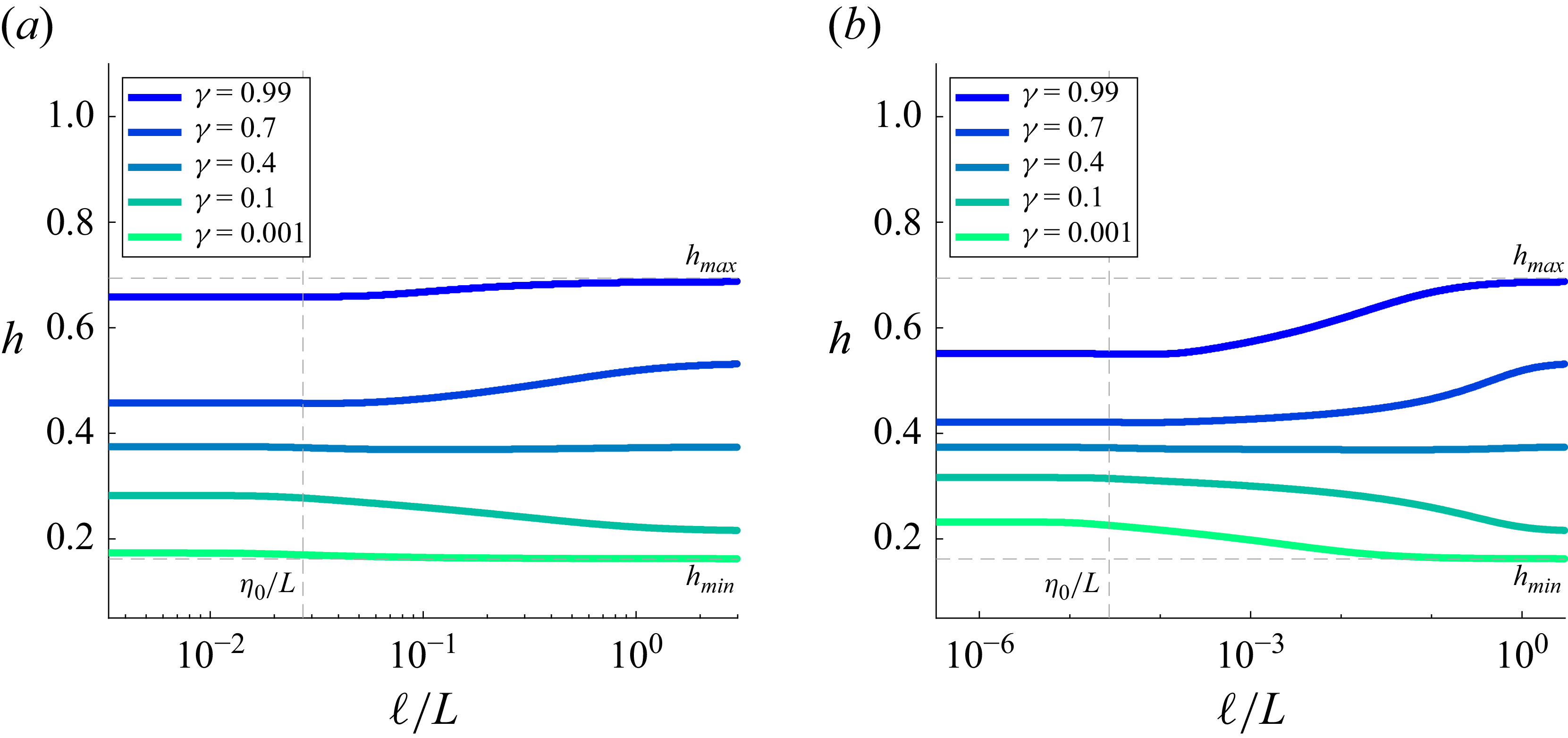
Variation of the Hölder exponent with separation distance of selected members of the ensemble are plotted for Reynolds numbers equal to (a)
 $10^4$
and (b)
 $10^8$
. We define
 $\eta _0 = \eta (h=1/3)$
to illustrate the onset of the dissipation range. For this figure, the Hölder exponent defining the transformation has a She–Lévêque singularity spectrum and varies from 0.162 to 0.694.

Another way of looking at our transform is to consider the different
 $h$
-values that a single
 $\gamma$
-value maps to across length scales. This is shown in figure 2 for two different Reynolds numbers. While
 $\gamma$
-values around
 $0.4$
correspond to almost constant
 $h$
-values, other
 $\gamma$
-curves cover a wider range of
 $h$
-values. It is this length dependence in the transform that allows us to encode multifractal statistics using a single distribution for
 $\gamma$
(in this case, the uniform distribution between
 $0$
and
 $1$
). Figure 2 shows that the variation with
 $\ell$
becomes more pronounced as the Reynolds number increases, since the transform has to accommodate very wide (at large scales) and very narrow (at small scales)
 $h$
-distributions.
5.2. Increment statistics
To illustrate how our ensemble of Gaussian fields exhibits multifractal features resembling the statistics of turbulence, we compute increment statistics by numerically evaluating (2.17). Longitudinal absolute-value increment p.d.f.s and structure functions from the model are compared with DNS data in figure 3 (we used the iso8192 dataset from the Johns Hopkins Turbulence Database (JHTDB), see Li et al. Reference Li, Perlman, Wan, Yang, Meneveau, Burns, Chen, Szalay and Eyink2008 for the database and see Yeung, Zhai & Sreenivasan Reference Yeung, Zhai and Sreenivasan2015 for the simulation details). Figure 3(a) shows that the model reproduces quantitatively the transition from close-to-Gaussian statistics at large scales to the heavy-tailed distributions characterising the small scales. The corresponding structure functions are shown in figure 3(b). Note that these are the unconditional structure functions predicted by the model, not to be confused with the
 $h$
- and
 $\gamma$
-dependent second-order functions
 $S(\ell ; h)$
and
 $\widetilde {S}(\ell ; \gamma )$
used to construct the model. Model parameters in (5.5), (5.6) were chosen to visually fit the
 $\langle |v|^2 \rangle /|\sigma _u|^2$
curve in figure 3(b). Their values are
 $\lambda = 2$
,
 $\textit{Re}_* = 82$
and
 $ L = 0.67 L_D$
, where
 $L_D$
is the integral length scale as reported in the iso8192 dataset. In figure 3(b), we observe a clear power law scaling in the inertial range matching the DNS data, as well as the proper asymptotic behaviour in the viscous and large scale cut-offs. We add that the exact functional form of the viscous transition may not capture all aspects of its DNS counterpart, but serves as a proof of concept and makes us confident that improved choices of
 $S(\ell ; h)$
and
 $\widetilde {S}(\ell ; \gamma )$
can capture a wide range of features of the data.
(a) The standardised velocity increment p.d.f. at various separation distances from the Gaussian ensemble (lines) plotted against simulation data at
 $Re_{\lambda} = 1285$
from the JHTDB iso8192 dataset (points). Additionally a standardised Gaussian is plotted in a red dashed line for reference. (b) The
 $n$
th-order structure function versus separation length (
 $\ell$
) from the Gaussian ensemble (lines) plotted against simulation data from the JHTDB iso8192 dataset (points). For this figure, the Hölder exponent defining the transformation has a She–Lévêque singularity spectrum and varies from 0.162 to 0.694. All curves and points are vertically shifted for clarity.

Scaling exponents of the even
 $n$
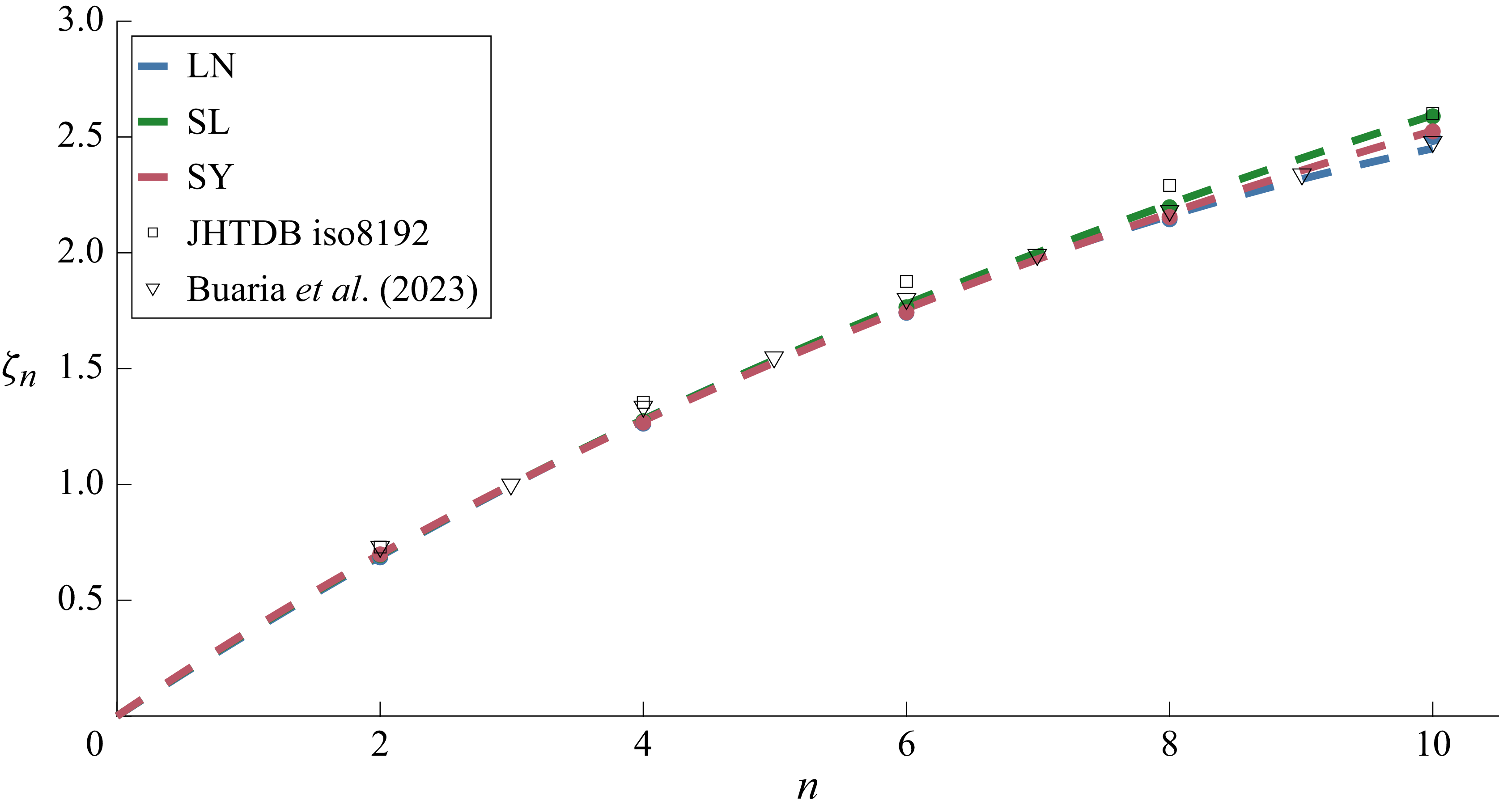
th-order structure functions for various singularity spectra – log-normal (LN), She–Lévêque (SL, She & Lévêque Reference She and Lévêque1994) and Sreenivasan–Yakhot (SY, Sreenivasan & Yakhot Reference Sreenivasan and Yakhot2021) – calculated from the Gaussian ensemble (coloured points) and compared with numerical calculations of (2.5), obtained from multifractal theory (colored dashed lines). The minimum and maximum Hölder exponents are set at the points where
 $D(h) =0$
. Additionally simulation data is plotted from the JHTDB iso8192 dataset (Li et al. Reference Li, Perlman, Wan, Yang, Meneveau, Burns, Chen, Szalay and Eyink2008; Yeung et al. Reference Yeung, Zhai and Sreenivasan2015) and Buaria & Sreenivasan (Reference Buaria and Sreenivasan2023).

By multiplying (2.17) with powers of the increments and integrating analytically, we get
 \begin{equation} \langle v^{n} \rangle = (n-1)!! \int _0^1 {\mathrm{d}} \gamma \, \widetilde {S}(\ell ; \gamma )^{n/2} \end{equation}
for even
 $n$
, which allows us to compute structure functions of any order directly from the second-order subensemble structure functions
 $\widetilde {S}(\ell ; \gamma )$
. With our change of variables, (3.7), one can show that the corresponding scaling exponents agree with (2.5). To check this numerically, we measure the scaling of the structure functions in (5.9) in the limit
 $\textit{Re} \rightarrow \infty$
. To this end, we choose an interval of length scales much smaller than
 $L$
. Then the best linear fit to a double logarithmic plot of (5.9) is used to compute
 $\zeta _n$
. In figure 4, we compare the exponents computed from the model’s structure functions (data points) to the exponents expected by the Legendre transform (2.5) (dashed lines), which agree reasonably well. This confirms that the ensemble of Gaussian fields constructed here is capable of reproducing the velocity increment scaling of various multifractal models.
5.3. Gradient statistics
Based on the full multi-scale description we introduced at the beginning of § 5, our model is able to predict gradient statistics as well. The tuning parameters (
 $\lambda$
,
 $\textit{Re}_*$
and
 $L$
) are set by matching the second-order structure function to data (see § 5.2). The gradient p.d.f., obtained from the functional with the right choice of the test function (2.18), is given by a superposition of Gaussian p.d.f.s, (2.20). The p.d.f. of the absolute value of the gradient is shown at different Reynolds numbers in figure 5(a), standardised by its variance, the average of (5.4).
(a) Standardised gradient p.d.f.s from the Gaussian ensemble (solid lines), alongside a standardised Gaussian (dashed line) for comparison. (b) The
 $n$
th-order standardised gradient moment from the Gaussian ensemble based on superposition of
 $\gamma$
((5.10), lines) plotted on top of calculations from the corresponding version of (5.10) based on superposition of Hölder exponents (points) versus Reynolds number. The Hölder exponents defining the transformation have a She–Lévêque singularity spectrum and vary from 0.162 to 0.694. The plots are vertically shifted for clarity.

Analogous to the increment moments, gradient moments can be computed by multiplying (2.20) with powers of the gradient and integrating analytically. As a result, gradient moments can be written as
 \begin{equation} \langle A^n \rangle = (n-1)!!\int _0^1 {\mathrm{d}} \gamma \left ( \frac {1}{2} \widetilde {S}''(0;\gamma ) \right )^{n/2} \!. \end{equation}
Again, this allows us to compute moments directly from the subensemble structure functions
 $\widetilde {S}(\ell ; \gamma )$
. We show the standardised moments,
 \begin{equation} M_n = \frac {\langle A^n \rangle }{\langle A^2 \rangle ^{n/2}} , \end{equation}
as a function of Reynolds number in figure 5(b) and compare them with a corresponding calculation made with an ensemble of Hölder exponents to demonstrate the validity of the model. They are expected to scale as a power of the Reynolds number,
 \begin{equation} M_n \sim \textit{Re}^{\xi _n}. \end{equation}
To check their scaling, we compute the exponents as linear best fits to the double logarithmic plot in figure 5(b). The result is shown in figure 6, and compared with data from a few different DNS and with the exponents obtained from multifractal theory (Nelkin Reference Nelkin1990),
 \begin{equation} \rho _n \approx - \min _h \frac {n(h-1)+1-D(h)}{1+h}, \qquad \xi _n = \rho _n - \frac {n}{2}\rho _2 . \end{equation}
The comparison with the expected exponents in figure 6 shows that they agree reasonably well. Again, this confirms that the Gaussian ensemble can reproduce multifractal statistics, also in the case of velocity gradients and their scaling with Reynolds number.
Reynolds number scalings of the standardised velocity gradient moments calculated from the Gaussian ensemble (coloured points) and from (5.13) (dashed curves) for the log-normal (LN), She–Lévêque (SL) and Sreenivasan–Yakhot (SY) singularity spectra. The minimum and maximum Hölder exponents are set at the points where
 $D(h) =0$
. DNS and experimental results.

6. Conclusion
The central contribution of this work is that it establishes a connection between multifractal models and functional approaches to turbulence based on ensembles of Gaussian fields. We developed an approach that promotes a multifractal model for increment statistics to a model for entire fields. This is accomplished by a change of variables that transforms a scale-dependent distribution of fluctuating Hölder exponents to a scale-independent distribution over the new parameter
 $\gamma$
. This allows for the superposition of Gaussian characteristic functionals parametrised on
 $\gamma$
, which then enables the computation of arbitrary field statistics, involving velocity, gradients or increments, for instance.
In the current work, we first demonstrated an analytically tractable instance of the transformation procedure that reproduces velocity increment statistics consistent with the log-normal model. After that, we introduced a more general form of the transformation that can encode multifractal increment and gradient statistics for any singularity spectrum
 $D(h)$
. The resulting characteristic functional can be used to model data from direct numerical simulations (or experiments).
Beyond the present work, the hope is that characteristic functionals, as constructed here, could also be helpful in the context of functional approaches to turbulence such as the Hopf equation (Hopf Reference Hopf1952), which is an elegant way to encode the field statistics of turbulence. A major open question towards this goal is the inclusion of skewness into the current framework, which is crucial to model the effects of self-advection and energy transfer across scales. Another topic for future investigation is the prediction of multiscale correlations of velocity increments (Benzi et al. Reference Benzi, Biferale and Toschi1998, Reference Benzi, Biferale, Ruiz-Chavarria, Ciliberto and Toschi1999; Friedrich et al. Reference Friedrich, Margazoglou, Biferale and Grauer2018) by the characteristic functional models constructed in this work.
Acknowledgements
We thank Jan Friedrich for helping us to establish the connection of our transform to their work. Additionally, we thank Mostafa Kamal for his simulation data used for the velocity gradient scaling exponent comparisons.
Funding
This project has received funding from the European Research Council (ERC) under the European Union’s Horizon 2020 research and innovation programme (Grant agreement No. 101001081).
Declaration of interests
The authors report no conflict of interest.
Appendix A. Connection to the ensemble by Friedrich et al. (Reference Friedrich, Peinke, Pumir and Grauer2021)
In their work on the explicit construction of joint multipoint statistics, Friedrich et al. (Reference Friedrich, Peinke, Pumir and Grauer2021) constructed an ensemble of characteristic functionals exhibiting statistics of the Kolmogorov–Obukhov model (K62; Kolmogorov Reference Kolmogorov1962; Obukhov Reference Obukhov1962). The K62 model is formulated in terms of
 $\varepsilon _\ell$
, the energy dissipation rate coarse-grained over scale
 $\ell$
. For simplicity, we focus on the inertial range,
 $\eta \ll \ell \ll L$
, with
 $\eta$
the classic Kolmogorov dissipative scale, independent of
 $h$
. Increment statistics in K62 can be implemented as a superposition of Gaussian distributions (Castaing et al. Reference Castaing, Gagne and Hopfinger1990; Friedrich Reference Friedrich2025),
 \begin{align} f_v(v; \ell ) &= \int \mathrm{d}\varepsilon _\ell \, f_\varepsilon (\varepsilon _\ell ; \ell ) g\!\left (v; S(\ell ; \varepsilon _\ell )\right )\!, \end{align}
with
 \begin{align} S(\ell ; \varepsilon _\ell ) &= U^2\! \left (\frac {\varepsilon _\ell }{\overline {\varepsilon }}\right )^{2/3} \left (\frac {\ell }{L}\right )^{2/3}\!. \end{align}
The distribution of
 $\varepsilon _\ell$
is assumed to be a scale-dependent log-normal distribution
 \begin{align} f_\varepsilon (\varepsilon _\ell ; \ell ) = \frac {1}{\varepsilon _\ell \sqrt {2\pi \sigma ^2(\ell )}} \exp \left (-\frac {(\log (\varepsilon _\ell ) - M(\ell ))^2}{2\sigma ^2(\ell )}\right ) \end{align}
with location parameter
 \begin{align} M(\ell ) = \log (\overline {\varepsilon }) - \frac {\sigma ^2(\ell )}{2} \end{align}
and scale parameter
 \begin{align} \sigma ^2(\ell ) = \mu \log \left (\frac {L}{\ell }\right )\!. \end{align}
The K62 model is equivalent to a multifractal model with quadratic singularity spectrum (2.6) and without bounds on
 $h$
. The difference is that
 $\varepsilon _\ell$
is used as a fluctuating parameter instead of
 $h$
. The equivalence can be seen by applying the transformation
 $\varepsilon _\ell = \overline {\varepsilon } (\ell /L )^{3h-1}$
to (2.2), (2.3) and (2.4), and setting
 $h_0 = 1/3 + \mu /6$
and
 $\sigma _h^2 = \mu /9$
while taking the inertial range limit.
With this in mind, we can apply the methodology outlined in § 3 to the K62 model, while replacing each instance of
 $h$
by
 $\varepsilon _\ell$
. In contrast to § 4, we choose a unit log-normal distribution for
 $\gamma$
, whose CDF is
 \begin{align} F_\gamma (\gamma ) = G(\log (\gamma )). \end{align}
The CDF of the fluctuating parameter
 $\varepsilon _\ell$
with scale-dependent p.d.f. (A3) reads
 \begin{align} F_{\varepsilon _\ell }(\varepsilon _\ell ; \ell ) = G\!\left (\frac {\log (\varepsilon _\ell ) - M(\ell )}{\sigma (\ell )}\right )\!. \end{align}
Then, the structure functions of the
 $\gamma$
-ensemble can be computed by (3.6) as
 \begin{align} \widetilde {S}(\ell ; \gamma ) &= S\left (\ell ; F_{\varepsilon _\ell }^{-1}(F_\gamma (\gamma ); \ell )\right ) \\[-12pt]\nonumber \end{align}
 \begin{align} &= U^2 \left (\frac {L}{\ell }\right )^{-2/3-\mu /3} \gamma ^{\frac 23 \sqrt {\mu \log \left (\frac {L}{\ell }\right )}}. \end{align}
This turns out to be the same inertial-range form of the structure function as proposed by Friedrich et al. (Reference Friedrich, Peinke, Pumir and Grauer2021). As the basis for their model, they use fractional Ornstein–Uhlenbeck processes with Hölder exponent
 $H=1/3$
. These are Gaussian processes with a specific, analytically known correlation function. For our considerations, it is only important to know that the corresponding structure function scales as
 \begin{align} S_{{K41}}(\ell ) \sim \ell ^{2H} = \ell ^{2/3} \end{align}
for
 $\ell \ll L$
, which is K41 scaling (Kolmogorov Reference Kolmogorov1941). Then, the subensemble structure functions (A9), which we obtained by application of our method to the K62 model, can also be obtained by applying the following length-scale transform to the K41 structure functions (A10):
 \begin{align} \ell \rightarrow \gamma ^{\sqrt {\mu \log \left (\frac {L}{\ell }\right )}} \left (\frac {L}{\ell }\right )^{-\mu /2} \ell. \end{align}
This is very close to the transform proposed by Friedrich et al. (Reference Friedrich, Peinke, Pumir and Grauer2021, (10)) for a fluctuating parameter
 $\xi \equiv \gamma$
. Overall, this means that the length scale transform proposed by Friedrich et al. (Reference Friedrich, Peinke, Pumir and Grauer2021) can be considered a special case of the more general transform presented here. However, choices regarding the small- and large-scale cut-off were made differently.
We also note that Friedrich et al. (Reference Friedrich, Peinke, Pumir and Grauer2021)’s work and the present framework share the property that a single sample field drawn from the probability distribution will only correspond to a single (random) value of the fluctuating parameter,
 $\xi$
or
 $\gamma$
, respectively. Hence, the full multifractal properties emerge only when averaging over multiple field realisations. To address this, an extension to the work by Friedrich et al. (Reference Friedrich, Peinke, Pumir and Grauer2021) has recently been proposed by Lübke et al. (Reference Lübke, Friedrich and Grauer2023), incorporating local fluctuations of the parameter. Adapting our framework in this way would be an interesting future direction to pursue.
Appendix B. Generalisation to vector fields
Our ensemble approach can be straightforwardly generalised to vector fields. To illustrate that, consider a three-dimensional incompressible velocity field
 $\boldsymbol u(\boldsymbol x)$
. Analogous to (2.11) the characteristic functional generalises to
 \begin{equation} \varPhi [\boldsymbol \alpha ; \gamma ] = \left \langle \exp \left [ \mathrm{i} \int _{-\infty }^{\infty } {\rm d}\boldsymbol{x} \, \alpha _i(\boldsymbol{x}) u_i(\boldsymbol{x}) \right ] \right \rangle \!, \end{equation}
where summation over repeated indices is implied and
 $\boldsymbol \alpha (\boldsymbol x)$
is a three-dimensional test function. If
 $\boldsymbol u(\boldsymbol x)$
is an incompressible statistically homogeneous Gaussian vector field with zero mean, its characteristic functional takes the form
 \begin{equation} \varPhi ^{G}[\boldsymbol \alpha ] = \exp \left [ -\frac {1}{2}\int _{-\infty }^{\infty } {\mathrm{d}} \boldsymbol x\int _{-\infty }^{\infty } {\mathrm{d}} \boldsymbol x' \alpha _i(\boldsymbol x) \widetilde C_{ij}(\boldsymbol x-\boldsymbol x';\gamma ) \alpha _j(\boldsymbol x') \right ]\!, \end{equation}
analogous to (2.12). Assuming statistical isotropy and incompressibility, the covariance tensor
 $\widetilde C_{ij}(\boldsymbol x-\boldsymbol x';\gamma ) = \langle u_i(\boldsymbol x) u_j(\boldsymbol x') \rangle$
can be written as (Pope Reference Pope2000)
 \begin{equation} \widetilde {C}_{ij}(\boldsymbol r;\gamma ) = \sigma _u^2 \left ( \left [ \tilde f(r; \gamma ) + \frac {1}{2} r \tilde f'(r;\gamma ) \right ]\delta _{ij} - \frac {1}{2} r \tilde f'(r;\gamma ) \, \hat r_i \hat r_j \right )\!, \end{equation}
where
 $\tilde f(r;\gamma )$
is the longitudinal velocity autocorrelation function, prime indicates a derivative with respect to
 $r$
;
 $\hat {\boldsymbol r}$
denotes the unit vector in the direction of
 $\boldsymbol r$
.
As a next step, we can relate the longitudinal autocorrelation function to the conditional structure function
 \begin{equation} \tilde f(r;\gamma ) = 1 - \frac {1}{2 \sigma _u^2} \tilde S(r;\gamma ), \end{equation}
which then allows to establish the relationship between a multifractal model for the increment p.d.f.s as outlined in § 3. Once the covariance tensor is determined this way, the Gaussian ensemble (2.13) straightforwardly generalises.
Quite obviously, addressing the question of how to include skewness into this framework is even more relevant for the generalisation to vectorial statistics. This is, however, beyond the scope of the current work.