INTRODUCTION
The introduction of genetically modified (GM) crops has been met across the globe with mixed views. Proponents argue that GM crops could herald a major breakthrough in the fight against famine and poverty (Delmer Reference Delmer2005), while critics point to the environmental and health risks as well as the mirage of thinking that complex issues such as poverty can be addressed with a single ‘magic bullet’ technology such as GM (Arends-Kuenning & Makundi Reference Arends-Kuenning and Makundi2000; deGrassi Reference deGrassi2003). Both sides in the debate have been adept at posting evidence and arguments to support their case, and much of it comprises claims and counter-claims of benefits and harm.
An excellent example of contradiction in the GM debate, and the one which will be explored in the present paper, can be found with ‘Bt’ cotton, having resistance to bollworm (Lepidoptera; Helicoverpa zea, Helicoverpa armigera, Diparopsis castenea, Earias biplaga and Earias insulana), a major constraint to cotton production (James Reference James2002). Bt cotton utilizes a gene from the bacterium Bacillus thuringiensis (Bt) that encodes for proteins (endotoxins) toxic to bollworm. Proponents argue that the use of plant resistance to control the bollworm means that less of the toxic (to non-target organisms, including humans), environmentally damaging and expensive insecticide can be used and this can have positive impacts on human health (Hossain et al. Reference Hossain, Pray, Lu, Huang and Fan2004). In addition, Bt-based resistance is an easier technology for the farmer, requiring far less labour to apply, and thus could make a contribution to integrated pest management (Hillocks Reference Hillocks2005). However, the presence of Bt-based resistance does not eliminate the need for insecticide, as older instars of the bollworm larvae are more able to tolerate the endotoxin (Russell & Deguine Reference Russell and Deguine2006). Some also argue that a reliance on a single-gene based resistance cannot be sustainable as the selection pressure can lead to pests which can overcome the resistance (Nuffield Council on Bioethics 2003; Kranthi & Kranthi Reference Kranthi and Kranthi2004; Jayaraman Reference Jayaraman2005; Russell & Deguine Reference Russell and Deguine2006). Proponents address this latter point by arguing that there are a number of forms of the Bt endotoxin (Gonzalez-Cabrera et al. Reference Gonzalez-Cabrera, Escriche, Tabashnik and Ferre2003) and this variation will allow breeders to ‘stack’ the genes and make the plant resistance more durable (Tabashnik et al. Reference Tabashnik, Patin, Dennehy, Liu, Carriere, Sims and Antilla2000).
There is a growing body of evidence which suggests that Bt cotton does provide substantial benefits for small-scale farmers in developing countries (James Reference James2002) and this includes India (Qaim Reference Qaim2003; Qaim & Zilberman Reference Qaim and Zilberman2003; Barwale et al. Reference Barwale, Gadwal, Zehr and Zehr2004; Bennett et al. Reference Bennett, Ismael, Kambhampati and Morse2004, Reference Bennett, Kambhampati, Morse and Ismael2006; Pemsl et al. Reference Pemsl, Waibel and Orphal2004; Morse et al. Reference Morse, Bennett and Ismael2005; Kambhampati et al. Reference Kambhampati, Morse, Bennett and Ismael2006; Crost et al. Reference Crost, Shankar, Bennett and Morse2007). These studies have suggested that growing Bt cotton can increase yield and quality as well as reduce insecticide and labour costs. More good quality cotton with less insecticide can improve the gross margin even when farmers have to pay a premium for Bt hybrid seed. Nevertheless, there are other reports to the contrary (Orton Reference Orton2003; Gala Reference Gala2005; Qaim et al. Reference Qaim, Subramanian, Naik and Zilberman2006) and critics have highlighted the problems of relying upon field trial-based data (it can be ‘unrepresentative’; Gala Reference Gala2005) and the difficulty of separating out a ‘Bt effect’ from an overall management effect given that adopters of the Bt hybrids are more likely to be the ‘better’ farmers (in terms of education, ability, interest, access to resources, etc.) within the community. The criticism can be summarized by the following quotation from one of the anti-GM groups: ‘The first adopters of Bt cotton were the farmers that were most able to weather such risks and overcome constraints: older farmers with additional non-farm income, more livestock and larger farms, in other words, the better-off farmers with access to credit. Another constraint for farmers is insecure land tenure as most farmers have access to tribal land only. Bt cotton has benefited better-off farmers and businessmen at the expense of the poor.’ (GMWatch 2005).
The implication is twofold. Firstly, that ‘better-off’ farmers will tend to be those that can benefit most from Bt cotton and, secondly, that when ‘economic benefit’ of Bt cotton is measured, this will be inflated as the best farmers are the ones adopting the new technology. Despite its obvious importance in a development context, this latter point in particular has received remarkably little attention in the Bt cotton literature. Researchers have typically tried to address it by collecting some limited ‘background’ information on the age, gender, education and household size of survey respondents and then using this information to see whether there are any obvious differences between adopters and non-adopters and then ‘control’ for these in terms of the economic results. Typical examples can be found in Bennett et al. (Reference Bennett, Ismael, Kambhampati and Morse2004, Reference Bennett, Kambhampati, Morse and Ismael2006) and Morse et al. (Reference Morse, Bennett and Ismael2005). Crost et al. (Reference Crost, Shankar, Bennett and Morse2007) state that many published farm-level studies do not control for such farmer self-selection and that efficient farmers do indeed adopt Bt cotton at a higher rate than their less efficient peers. Crost et al. (Reference Crost, Shankar, Bennett and Morse2007) point out that the more efficient farmers will be better managers, able to get higher yields through management, and thus there is a ‘farmer’ effect when the economic impact of Bt cotton is assessed. They employed two models, one based on pooled effects and the other based on fixed effects, in order to test for such a ‘farmer’ effect and come to the conclusion that it can account for more than half of the recorded yield benefit of growing Bt cotton in India. However, while the study by Crost et al. (Reference Crost, Shankar, Bennett and Morse2007) is one of the few attempts to primarily focus on the ‘farmer’ effect in an analysis of Bt economic impact, it does not explore in depth the reasons for such an effect and neither does it focus on the variable that arguably is the most apparent and relevant to the farmer, namely gross margin.
The aim of the present paper is to explore the ‘farmer’ effect in greater depth as part of the economic impact of growing Bt cotton in India. The paper examines how much of any benefit (if it exists) to adopters of Bt cotton can be ascribed to the Bt engendered resistance and how much is due to adopters perhaps being ‘better’ farmers or having access to more resources. In addition if there is a ‘farmer’ effect, the paper will consider the important elements that comprise it.
MATERIALS AND METHODS
The survey was conducted in the district of Jalgaon, situated in the north of Maharashtra State, India. Located within a productive, irrigated agricultural region, Jalgaon is a significant collection and distribution centre of agricultural goods. The leading products are millet and raw cotton and the region's rich volcanic soil is particularly well-suited to cotton production. Jalgaon is an important centre for cotton-textile and vegetable-oil mills, particularly groundnut-oil and hydrogenation plants. With an area of about 11,700 km2, Jalgaon District has a population of about 4 million. Jalgaon is divided into 15 sub-districts known as Talukas and has 1475 villages. It has a minimum temperature of 20°C and a maximum of 35°C with an annual rainfall of 763 mm. The main crops grown in Jalgaon are banana, cotton, sugarcane, oil seeds and pulses. Cotton is planted 2–3 weeks prior to the monsoon season in June and harvested in November and December.
There are two species of cotton grown in Jalgaon: Gossypium hirsutum and Gossypium arboreum. Most of the cotton grown (0·73 of cotton area) is an intra-hirsutum hybrid, with the remainder being covered with improved (non-hybrid) G. hirsutum and G. arboreum cultivars. Bt hybrids were commercially introduced in the 2002 growing season. Three Mahyco–Monsanto Bt cotton hybrids were introduced: MECH-162 Bt, MECH-184 Bt and MECH-12 Bt. Popular non-Bt varieties are Bunny, Tulsi, NHH-44 and JK-666.
A questionnaire-based survey of 450 cotton producers in two Talukas, Parola and Darangaon, in Jalgaon district was undertaken during April and May 2004. The questionnaire focused on the first two cotton-growing seasons (2002 and 2003) following the commercial introduction of Bt hybrid. The essence of the questionnaire was to capture information on cotton producer's background, their perception of Bt cotton, cultivation practices (e.g. cotton varieties planted, cotton output, output prices and uses and cost of inputs) and as well as capital and assets, financial profile and impacts of Bt cotton on their livelihood. Experienced personnel who had previously conducted a similar study of Bt cotton interviewed cotton producers at length. In addition, the interviewers were trained for 2 days and conducted a pilot study on three cotton producers who were not included in the sample.
The respondents were classified into ‘adopters’ of Bt cotton (i.e. those who had planted at least one plot of Bt cotton in season 2002 and/or 2003; thus a farmer who had planted a plot of Bt cotton in 2002 but not in 2003 was still classified as an ‘adopter’) and ‘non-adopters’ (i.e. those who had not planted a plot of Bt cotton in either 2002 or 2003). Adopters made up the majority of the sample (300 respondents), largely because the Bt hybrids had become so popular in the area. Non-adopters numbered 150. All respondents were selected randomly.
For each respondent, two types of information were collected: firstly, background information on the household (e.g. size, labour availability, asset ownership, crops grown, income, credit and savings) and respondent (e.g. age, education and years of farming experience) and, secondly, detailed production information on at least one plot of cotton owned by the household in 2002 and 2003. For non-adopters the plots would, of course, only be for non-Bt varieties. Where possible for adopters, plots of Bt and non-Bt were sampled for the same respondent. This provides some ‘control’ for a number of producer-related factors that might influence performance of the technology (such as entrepreneurial ability, age, experience and expertise in growing the crop and access to other inputs such as credit and irrigation). In some cases where the whole farm was planted to Bt cotton, this was not possible. The original sample comprised a total of 932 cotton plots for the two cotton seasons. Data collected included yield, plot size, amount and value of inputs used (including labour) and value of yield. The income and expenditure data were used to calculate gross margin (defined as output value−variable costs).
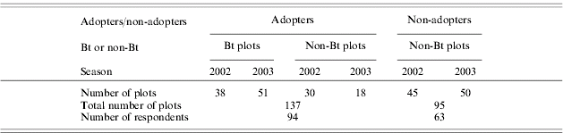
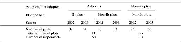
However, problems emerged with the original sampling frame of 450 respondents and 932 cotton plots because, although paper records were consulted whenever possible, much was dependent upon their memory. While respondents generally had good knowledge of plot outputs and inputs such as pesticide, there were often problems with their recollection of the labour used for cotton cultivation. Thus a respondent might remember labour input for some practices but not others, or might be uncertain. In order to avoid any bias that could emerge with incomplete datasets, it was decided that only the complete records available for respondents and plots would be included in the analysis. This set totalled 137 plots of 94 adopting households (Bt as well as non-Bt) and 95 plots of 63 non-adopting households. For these plots, labour involved in all activities, as well as other inputs and outputs, were known with some certainty. The final sample of checked and validated records was stratified as shown in Table 1.
Stratification of respondents and cotton plots
Data analysis was centred on comparisons between adopters and non-adopters – respondents and plots. The comparison was via a one-way analysis of variance (ANOVA), and all data were transformed by logarithms (z=loge (x) or Z=loge (x+1)). The critical level for significance was taken as P⩽0·05, but comparisons in which 0·05<P<0·10 are also reported where applicable. This method of analysis (as distinct from a production function approach as adopted by Crost et al. Reference Crost, Shankar, Bennett and Morse2007) allows for a comparison of performance as it would be perceived by the farmers. For plots, the comparison also included seasons (2002 v. 2003) and an interaction between adoption and season.
RESULTS
Comparisons of respondents
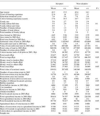
In terms of general background features of the farmer and household, only a few differences were discernible between adopters and non-adopters of Bt cotton, but these are clearly important (Table 2). With regard to age, farming experience and education of respondent, there were no significant differences between adopters and non-adopters. In terms of household family labour, there was some suggestion (P<0·1) that adopters had more full-time and male labour available for agriculture than did the non-adopters. Given that crop cultivation in this area is dependent on human and animal labour, this is a major advantage.
Characteristics of adopters and non-adopters of Bt cotton (mean and standard deviation)
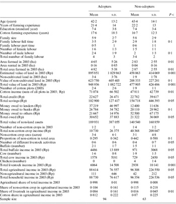
Comparisons were made with a one-way ANOVA and the series were logged to correct non-normality. The probability value is only given for significant differences.
The pattern of credit for farming activities was much the same for both adopters and non-adopters. However, once credit in general is considered (i.e. the total owed not just for agriculture but for activities such as education, health care, buildings, etc.) then adopters have significantly more credit (Rupees (Rp) 30 652) than do non-adopters (Rp 21 322).
With regard to land, there were a number of significant differences between adopters and non-adopters. Generally, adopters had more land in terms of both area and financial value (cultivated and not cultivated) than non-adopters. The difference was quite marked – an average of 1·82 ha per respondent more for adopters compared to non-adopters. Also, while the difference was not statistically significant there is some suggestion that adopters had more cotton plots than non-adopters. In terms of income from cotton, the average difference between adopters and non-adopters was over Rp 23 000.
For non-cotton crops, it would appear that adopters and non-adopters are similar in terms of the number of non-cotton crops grown and the average acreage allocated to such crops. But because adopters have larger cultivated areas, the proportion of land allocated to non-cotton crops was significantly higher for non-adopters (0·44) compared to adopters (0·30). Interestingly non-adopters reported a much greater (but not statistically significant) level of income from non-cotton crops compared to adopters. Thus, it would seem that the non-adopters did better on much the same area of non-cotton.
Another set of significant differences between adopters and non-adopters was with livestock. In general, adopters were involved in more livestock activities and had twice as much income from livestock (especially with buffalo and cows) than did non-adopters. This difference helps explain the greater area of land farmed for adopters.
Overall, while adopters did best with cotton and livestock, non-adopters did well with non-cotton crops. Indeed, income from agriculture was significantly higher for non-adopters and given that the bulk of household income is from agriculture then household income was also significantly higher for non-adopters. This suggests that the categories of adopter and non-adopter may reflect two quite different types of farmer. Adopters concentrate more on cotton, and have more land and higher incomes from livestock. Non-adopters are generalists in terms of the crops that they grow, and have less land and less of an emphasis on cotton.
Comparisons of plots
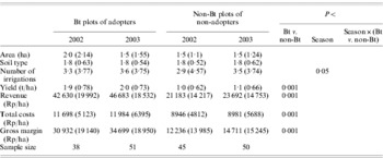
The results of comparing cotton production on Bt plots of adopters with non-Bt plots of non-adopters calculated on a per hectare basis are shown in Table 3. For both seasons, the yield of the Bt plots was significantly greater (c. 80%) than for those of non-Bt plots of non-adopters and, combined with a better quality of Bt cotton, this resulted in double the revenue. Total costs for Bt were higher than non-Bt, but overall the gross margin of Bt plots was significantly higher than non-Bt; this was generated by the higher revenue of those plots and not by reduced costs. However, given that the two groups of farmer have differences as shown in Table 2, it is important to establish how much of the higher yield of Bt plots is due to the variety (i.e. a genetic effect) and how much is due to a better environment resulting from better management.
Comparison of cotton-related costs, revenue and gross margin per acre between Bt plots of adopters and non-Bt plots of non-adopters

For each variable is given: mean and standard deviation in parentheses. Values have been logged (z=ln (x+1)) before ANOVA. The probability value is only given for significant differences.
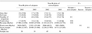
One comparison that would help elucidate the ‘farmer’ effect would be to compare non-Bt plots of adopters and non-adopters. Here, of course, the genetic effect of Bt is discounted. The results (Table 4) do appear to support the hypothesis that Bt farmers can generate significantly higher yields (29–43% higher) and revenues (31–47% higher) from non-Bt cotton. However, while the gross margins of Bt adopters seemed higher than non-Bt in both seasons the differences were not statistically significant (sample variation was high).
Comparison of cotton-related costs, revenue and gross margin per acre between non-Bt plots of adopters and non-adopters

For each variable is given: mean and standard deviation in parentheses. Values have been logged (z=ln (x+1)) before ANOVA. The probability value is only given for significant differences.
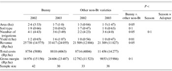
It is important to determine what has contributed to this improved performance of adopters relative to non-adopters even with non-Bt plots. One obvious difference rests with the non-Bt variety grown by adopters and non-adopters. The variety Bunny is especially popular among Bt adopters compared to non-adopters. Of the 48 non-Bt plots grown by Bt adopters, 34 (0·71) were planted to Bunny, whereas of the 95 ‘non-Bt’ plots of non-adopters only 38 (0·40) were Bunny. The results in Table 5 compare the performance of plots of Bunny with other plots of non-Bt for both adopters and non-adopters. Bunny has a significantly greater yield (P<0·01) and revenue (P<0·05) than other non-Bt types and total costs are much the same, given that all non-Bt varieties have to be sprayed with insecticide. As a result, the gross margin of Bunny is significantly higher (P<0·1) than other non-Bt varieties.
Comparison of cotton-related costs, revenue and gross margin per acre between plots of Bunny variety and other non-Bt cotton varieties

For each variable is given: mean and standard deviation in parentheses. Values have been logged (z=ln (x+1)) before ANOVA. The probability value is only given for significant differences.
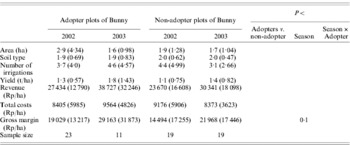
While differential planting of Bunny itself provides a significant advantage for Bt adopters, it is necessary to examine whether there is any evidence that adopters of Bt are ‘better’ at farming Bunny compared to non-Bt. In other words, once the genetic advantage of Bunny has been discounted, farmers may be achieving very similar outputs. The results of this comparison are shown in Table 6 and, while the average yield and revenue of Bunny plots for adopters are higher than for non-adopters in both 2002 and 2003, none of the differences is significant. However, sample sizes for this comparison are low and it is certainly possible that adopters consistently outperform non-adopters in these seasons.
Comparison of cotton-related costs, revenue and gross margin per acre between plots of Bunny variety produced by adopters and non-adopters of Bt cotton

For each variable is given: mean and standard deviation in parentheses. Values have been logged (z=ln (x+1)) before ANOVA. The probability value is only given for significant differences.
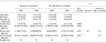
Another means of addressing the problem highlighted above with regard to comparing Bt plots and non-Bt plots of different farmers is to compare Bt and non-Bt plots of adopters only (Table 7). This comparison, of course, does not allow for the direct estimation of a ‘farmer’ effect (in terms of comparing adopters and non-adopters) but does allow for an estimation of the Bt advantage as it would be perceived by the farmers. The results suggest that there is indeed a positive gain from growing Bt. Bt plots are higher yielding (27–42% higher) and have higher revenues (34–53% higher) than non-Bt, although costs are higher for Bt. Overall the gross margins of Bt plots are significantly higher (59–66% higher) than non-Bt. However, it should be remembered that the non-Bt plots of adopters are mostly the Bunny variety and this variety is itself better-performing than other non-Bt types. Therefore, these farmers are seeing the benefit of Bt relative to one of the best non-Bt varieties. There are some significant interactions between season and variety (P<0·1) for total costs and gross margin, but this should not be surprising given that bollworm pest pressure will vary over seasons.
Comparison of cotton-related costs, revenue and gross margin per acre between Bt and non-Bt plots of adopters

For each variable is given: mean and standard deviation in parentheses. Values have been logged (z=ln (x+1)) before ANOVA. The probability value is only given for significant differences.
DISCUSSION
The results presented in this paper provide further support for the broad body of evidence that points to an economic advantage for Bt cotton in India (Qaim Reference Qaim2003; Qaim & Zilberman Reference Qaim and Zilberman2003; Barwale et al. Reference Barwale, Gadwal, Zehr and Zehr2004; Bennett et al. Reference Bennett, Ismael, Kambhampati and Morse2004, Reference Bennett, Kambhampati, Morse and Ismael2006; Pemsl et al. Reference Pemsl, Waibel and Orphal2004; Morse et al. Reference Morse, Bennett and Ismael2005; Kambhampati et al. Reference Kambhampati, Morse, Bennett and Ismael2006; Crost et al. Reference Crost, Shankar, Bennett and Morse2007). The yield of Bt cotton was c. 80% higher than non-Bt and hence resulted in greater revenue and while costs were also higher, the overall effect was that gross margin for Bt was significantly higher than that of non-Bt. These findings agree with those of Crost et al. (Reference Crost, Shankar, Bennett and Morse2007), also employing data from India, who found a 92% increase in yield for Bt plots compared to non-Bt based on a pooled effects regression model. However, as Crost et al. (Reference Crost, Shankar, Bennett and Morse2007) reiterate, some of the reported yield advantages of Bt cotton over non-Bt in a number of countries have been lower than this; ranging from 6 to 65%.
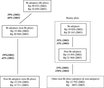
However, it is important to establish how much of this economic gain, as perceived by the farmers themselves, from growing Bt is due to a ‘farmer’ effect and how much is due to the Bt trait. Crost et al. (Reference Crost, Shankar, Bennett and Morse2007) provide a clue in that they also employed a fixed effects model which suggested that the yield advantage of Bt over non-Bt was 31%; a third of the estimate based on a pooled effects model. The fixed effects model controls for farmer selection bias and hence they conclude that there is a significant self-selection effect which explains more than half of the observed increase in yield of 92% for plots of Bt over non-Bt. Using gross margin, the variable that arguably means most to the households in the sample, as the basis for the assessment, the data in Tables 3–7 for 2002 and 2003 can be summarized as in Fig. 1. The main component of Fig. 1 on the left-hand side shows the increase in gross margin from non-Bt plots of non-adopters through non-Bt plots of adopters and at the top of the chain, Bt plots of adopters. A ‘farmer’ effect can be discerned by comparing non-Bt plots of adopters and non-adopters. The assumption is that the observed benefit in gross margin (42–59%) for adopters could be the result of better management or the adoption of better non-Bt varieties such as Bunny. Given that there are differences between the two categories of respondents in a range of factors such as household labour and livestock then this is a reasonable assumption. Comparing Bt and non-Bt plots of adopters provides a further increase in gross margin (59–66%) for the Bt plots. Indeed, it is interesting that the average increase for these two links in the chain is much the same. The overall effect, therefore, is that when comparing Bt plots of adopters and non-Bt plots of non-adopters, roughly half the observed increase is due to a ‘farmer effect’ and half to the Bt trait. This is a conclusion broadly in line with that of Crost et al. (Reference Crost, Shankar, Bennett and Morse2007).
Plot comparisons (based on average gross margin, Rupees/ha) as would be perceived by the farmers comprising the Jalgaon sample.

It remains to be examined what has caused this ‘farmer’ effect with gross margin. In the present case it is largely due to the fact that Bt adopters also tend to plant high-performing varieties of non-Bt, namely Bunny. The yield benefit in growing Bunny compared to other non-Bt varieties was noted by Crost et al. (Reference Crost, Shankar, Bennett and Morse2007). The ‘Bunny’ effect is demonstrated in the right-hand side of Fig. 1. The Bunny variety had a significantly higher (P<0·1) gross margin than other non-Bt varieties. However, while gross margin was higher (by 31 and 33%) for adopters growing Bunny compared to non-adopters growing Bunny in both 2002 and 2003, the differences were not statistically significant. Thus, much of the difference in gross margin between non-Bt plots of adopters and non-adopters can be explained by the preferential planting of Bunny by adopters, although there is also likely to be a ‘better’ management component.
‘Adopters’ of the technology in the first two seasons following commercial release are indeed quite different from ‘non-adopters’ in a number of ways and in its broadest sense this supports the points made in the quotation given earlier (GMWatch 2005). While there is no evidence from the present data that early adopters are older or more experienced than non-adopters, there were important differences in important aspects such as family labour, land area owned and amount of credit taken. Most important of all it would appear that adopters are farmers who specialize more on cotton; at least in terms of the land area they devote to the crop. However, while there is a ‘farmer’ effect, the data point conclusively towards there also being a clear economic advantage to growing Bt cotton. The comparisons that need to be made in GM-impact studies are of critical importance. Comparing Bt and non-Bt plots of different farmers can be misleading (the Bt effect can be inflated) if no account is taken of the fact that adopters can be different from non-adopters in a number of ways.
CONCLUSION
What and how comparisons are made is of critical importance in judging the success of any agricultural technology, and GM is no different. Indeed if anything the issue is raised to a greater level of sensitivity because of the highly contested nature of the technology as ‘positive’ or ‘negative’. Critics have claimed that much of the reported ‘benefits’ from GM crops arise because adopters are simply better farmers, and the present paper does provide some limited evidence in support of this viewpoint. As can be seen with Bunny, even non-GM varieties can provide significant economic benefits. However, while a ‘farmer’ effect provides a partial explanation for a Bt advantage the evidence from the present work suggests that the bulk of the gross margin difference (59–66%) seen between Bt and non-Bt varieties in this study is a result of the Bt gene. A difference of this magnitude with a variable, gross margin, of such importance to households readily explains the popularity of Bt cotton in this part of India.
The authors thank Mahyco and ACNielsen ORG-MARG for access to the data they have collected in India. They also thank Mr Jagresh Rana for logistic support and Mr Matthieu Arnoult for help with data analysis. They also thank the anonymous referees for their comments and suggestions for the improvement of this paper. Data analysis was funded by the United Kingdom's Department for International Development (DFID) (project ‘Monitoring the impact of GM cotton in India’ MC/GEA/004). The views expressed are not necessarily those of DFID.