Introduction

An understanding of basal motion is essential to many studies of glacier dynamics, including those of ice-stream flow, glacier surges and seasonal and short-term velocity fluctuations. However, the difficulties of directly observing the basal interface have left the mechanisms of such motion obscure, and our understanding of the processes occurring at the bed is still far from complete. Boreholes, caws and tunnels provide a means to observe the bed on a local scale, but they are often logistically unfeasible, and can affect the dynamics. For instance, a single borehole is not a reliable indicator of the spatial extern of subglacial changes, and it may disturb the existing subglacial drainage system by introducing a new source for basal water. Aside from these localized measurements, the bed of a glacier can be investigated only after the ice leaves, or it may be imaged by geophysical methods such as electromagnetic or seismic sounding.

Seismic techniques have been used as a non-invasive method to investigate basal motion over large areas on a variety of glaciers. For example, passive seismic techniques have been used to measure the extent and nature of sub-glacial and englacial seismic events related to glacier motion on Ice Streams B and C, West Antarctica (Reference Anandakrishnan and AlleyAnandakrishnan and Alley, 1997), and Variegated Glacier, Alaska, U.S.A. (Reference Raymond and MaloneRaymond and Malone, 1986), as well as to monitor events related to iceberg calving (e.g. Reference Wolf and DaviesWolf and Davies, 1986). Active seismic measurements of ice thickness, using explosive sources, have been used to estimate the deformational component of glacier speed, and thus infer the component of motion at the bed, on Taku Glacier, Alaska (Reference Nolan, Motyka, Echelmeyer and TrabantNolan and others, 1995), and Jakobshavn Isbræ, Greenland (Reference Clarke and EchelmeyerClarke and Echelmeyer, 1996). Active seismic methods have also been used to investigate basal and englacial layer properties over extensive regions of Antarctica (e.g. Reference Bentley and CraryBentley, 1971). Similar methods have been employed to determine the thickness, porosity and effective pressure of subglacial tillsFootnote ^* beneath Ice Stream B (Reference Blankenship, Bentley, Rooney and AlleyBlankenship and others, 1987), as well as their spatial variation (Reference Blankenship, Bentley, Rooney and AlleyRooney and others, 1987; Reference Atre and BentleyAtre and Bentley, 1993). Such measurements have also been made on Rutford Ice Stream, Antarctica (Reference SmithSmith, 1997). In a study similar to ours, seismic reflection methods have been used to observe changes that occurred between pre-surge and surge conditions at the bed of Variegated Glacier (Reference RichardsRichards, 1988).

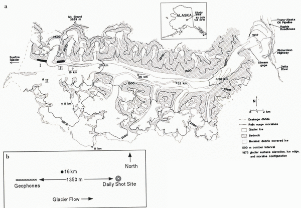
In 1993 we applied seismic reflection techniques to investigate changes at the bed of Black Rapids Glacier, Alaska (Fig. 1), during its annual spring speed-up, and during subsequent short-term velocity fluctuations. This glacier was selected for study because it has a well-documented history of large seasonal changes in basal motion (Reference Heinrichs, Mayo, Echelmeyer and HarrisonHeinrichs and others, 1996; personal communication from W. Harrison, 1993). These seasonal changes appeared to occur on a reliable schedule, and our intent was to study the nature and extent of concomitant changes at the bed by comparing the properties of reflected seismic waves before, during and after this speed-up. The repeated measurements were made at a high temporal resolution to pinpoint the timing and location of basal changes, and thus to increase our understanding of the mechanisms of motion at the glacier bed.

Our study was part of a larger project in which researchers from the University of Washington, Seattle, U.S.A., conducted analogous radio-echo sounding (RES) investigations (Reference GadesGades, 1998), and the outlet stream of the glacier was monitored for hydrological parameters (Reference CochranCochran, 1995).

Fig. 1

(a) Map of Black Rapids Glacier, Alaska. The glacier is shown with its center-line coordinates, beginning with 0 km at the head. Lake locations are labeled with Roman numerals in the order that they drained in summer 1993. (b) An enlargement of the 16 km study area.

From mid-May to mid-July, coincident with the geophysical research, we surveyed ice motion twice daily (including three-dimensional position and horizontal strain over 5 km); measured vertical strain and passive seismicity hourly near the survey site; monitored the outlet stream for stage, conductivity and turbidity using automated equipment; and occupied a stream camp continuously for related studies. These data provide the background against which comparisons of the geophysical data will be made. In this paper we present only the seismic techniques and observations, focusing on their spatial and temporal changes. In the companion paper (Reference Nolan and EchelmeyerNolan and Echelmeyer, 1999; denoted as N&E) we give an interpretation of these seismic-observations in terms of subglacial morphology and the mechanisms of seismic change.

Black Rapids Glacier: Motion History and Drainage Events

Black Rapids Glacier is a surge-type glacier in the central Alaska Range. Much of it lies in an east–west valley along the Denali Fault, a major tectonic fault extending for several hundred km through the Alaska Range. Motion along this predominantly strike slip fault has placed granitic rocks adjacent to metasediments across the fault (Reference NoklebergNokleberg and others, 1992) and has caused a loss of competency of the rocks directly on the fault. It is interesting that three other large surge-type glaciers (Susitna, West Fork and Yanert Glaciers) lie along this fault just to the west (Reference Harrison, Echelmeyer, Chacho, Raymond and BenedictHarrison and others, 1994); these glaciers appear to surge every 50–70 years (Reference ClarkeClarke, 1991).

The glacier is about 43 km long, with an area of 246 km². It flows from an elevation of about 2500 m to a terminus at about 1000 m, with an average surface slope of about 2.3^° (Reference Heinrichs, Mayo, Echelmeyer and HarrisonHeinrichs and others, 1996). Center-line ice thickness is about 630 m near our field site (Fig. 1). The glacier is temperate (Reference Harrison, Mayo, Trabant, Weller and BowlingHarrison and others, 1975), and it is situated in the cold, dry continental climatic regime characteristic of interior Alaska.

Black Rapids Glacier last surged in 1936–37 (Reference HanceHance, 1937), and relic moraines indicate that previous surges have crossed the current location of the Trans-Alaska Pipeline and a major highway (Reference Reger, Sturmann, Beget, Solie and TannianReger and others, 1993), closing off the valley and damming the Delta River (Fig. 1). Since its last surge, the glacier has thinned by up to 220 m near the terminus, while thickening by about 50 m on the upper glacier (K. Echelmeyer and W. Harrison, unpublished data, 1996).

Average center-line surface speeds in the neighborhood of our field site (Fig. 1) are about 55–65 m a^-1. Based on a 20 year record of surveying (Reference Heinrichs, Mayo, Echelmeyer and HarrisonHeinrichs and others, 1996) and 15 years of time-lapse photography (personal communication from W. Harrison, 1993), we know that the average annual velocity in the region between 14 and 20 km (Fig. 1) varies by about 50% (30 m a^-1), possibly periodically. The seasonal fluctuations in speed mentioned above are superimposed on these longer-term variations, with speeds in spring and early summer being about 100–300% faster than those in winter, as averaged over a few weeks. The spring transition in speed occurs abruptly within about 1 day, and the velocity generally remains high for 2–4 weeks. Afterwards there is a slow decay to a minimum in late summer, followed by a gradual increase through the winter. This spring speed-up usually occurs between 1 and 10 June. All of these variations in speed are due primarily to changes in basal motion (Reference Heinrichs, Mayo, Echelmeyer and HarrisonHeinrichs and others, 1996).

Unfortunately, in 1993 the spring speed-up occurred about two and a half weeks earlier than expected (22 May), on the day that our seismic monitoring began. However, during the subsequent measurement period we observed three jökulhlaupsFootnote ^* up-glacier of our monitoring site. Associated with each jökulhlaup was a period of increased glacier speed, with up to a four-fold increase in speed during each event, as welt as up to 15 cm increases in surface elevation (Fig. 2). The high speeds lasted about 1 day each, while the elevation changes varied in duration (Fig. 2). Such events appear to be annual phenomena (Reference Sturm and CosgroveSturm and Cosgrove, 1990; Reference Raymond, Benedict, Harrison, Echelmeyer and SturmRaymond and others, 1995; Reference Truffer, Harrison, Echelmeyer and HeinrichsTruffer and others, 1996). For a period of about 45 days encompassing these events, we made nearly daily seismic reflection surveys of one section of the bed that was affected by these transient water inputs. This paper describes the seismically detected changes at the bed that occurred during these events.

Fig. 2.

Surveyed speed of Black Rapids Glacier near 16 km in 1993. The initial spring speed-up occurred about day 142 (22 May), following a storm. The three peaks in speed labeled with Roman numerals correspond to drainage of the lakes identified in Figure 1. Elevation change is calculated from the vertical coordinate minus the mean decrease throughout the summer due to surface slope.

The three jökulhlaups varied in size, location, drainage method and glacier-dynamic effects. We observed the first and third jökulhlaups, located at ice-marginal lakes on the north side of the valley (labeled I and III in Fig. 1), and afterwards completed maps of their empty basins. About 10⁶ m³ of highly turbid water drained from each. The second jökulhlaup, located at a supraglacial pothole (II in Fig. 1), was not directly observed nor was its basin surveyed afterwards. No more than about 10⁵ m³ of clean meltwater drained from this pothole, but other nearby potholes may also have drained at the same lime.

Seismic Background and Methods

Wave Types and Speeds

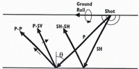
Seismic waves are characterized by the type of particle motion they induce through a medium (Fig. 3). The direction of particle motion for compressional (P) waves is the same as wave propagation, whereas for shear (S) waves it is perpendicular. S-wave particle motion can be decomposed into vertical (SV) and horizonal (SH) polarizations.

Upon reflection of a P-wave at non-normal incidence, some of the incident energy is converted to SV motion (Fig. 3), and vice versa SH motion does not undergo such conversion. Unlike P-waves, S-waves are often difficult to generate with explosives, and thus converted P-to-SV (P-SV) reflections may be the only means to study S-wave response. This was true in our study: no useful S-waves were generated by our sources.

Fig. 3.

Schematic of seismic waves. Heavy arrows show direction of wave propagations; light arrows show direction of particle motion. SH particle motion is into and out of the page.

In addition to these reflected and converted waves, two direct waves (traveling from the source to the geophones along the ice surface) are often recorded: a direct P-wave and a Rayleigh wave (also known as “ground roll”). The latter is considered coherent noise in this study.

The speeds of P-and S-waves, V _P and V _S, respectively, in temperate ice are not well constrained. They are sensitive to the amount of liquid water at the grain boundaries (Reference RöthlisbergerRöthlisberger, 1972). The speeds in colder ice, where little water is present, are much better determined. The wave speeds for temperate ice that we use in this paper were derived from data obtained during our project, as described in Appendix A. In particular, we found an average P-wave speed of V _P = 3704 m s^-1, which is at the upper end of the range recommended by Röthlisberger (1972, p. 20) of 3600–3700 m s^-1.

Wave Identification and Reflector Migration

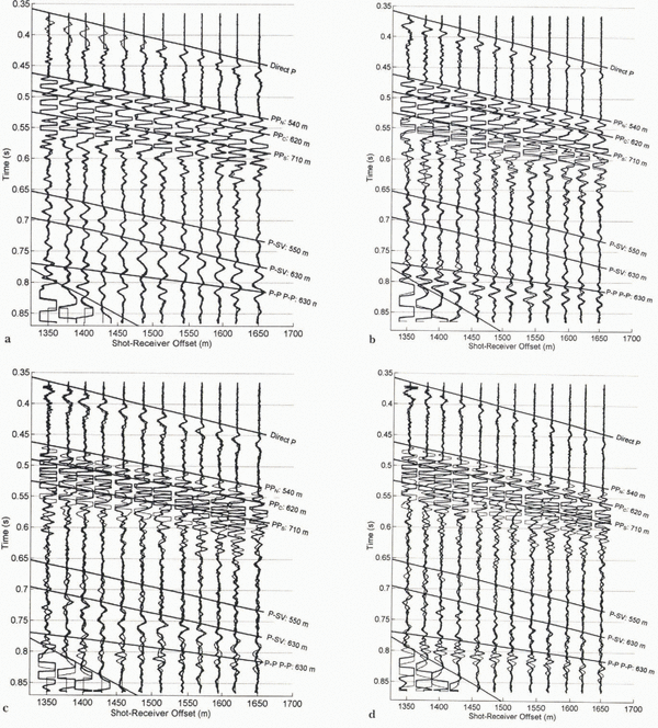
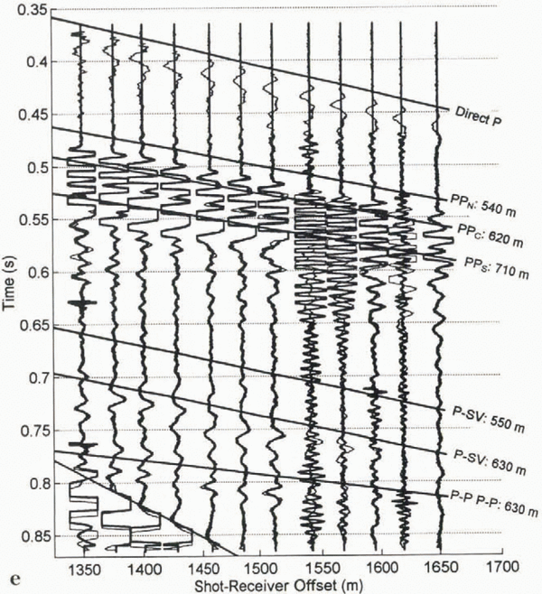
We were able to identify the type of waves present by comparing the arrival times of the observed waves along the geophone spread (the so-called “move-out”) to theoretical time distance curves (also known as travel-time curves). Preliminary identification was made in the field using a normalized time–distance chart (Reference RöthlisbergerRöthlisberger, 1972). The seismograms in Figure 4 are examples of our longitudinal data. The superimposed time–distance curves were calculated using a simple geometry with ice of a uniform thickness over bedrock. We used these curves to identify the most coherent P-P, P-SV, and multiple P-P (P-P P-P) waves in the seismograms, as well as the direct P-wave and ground roll. As can be seen in these figures, there are often several waves of each type in the longitudinal sections. They come from different parts of the valley bottom and walls, as identified below. This multitude of different waves is a feature of seismic reflection studies on valley glaciers, due to the bed’s curved shape, and is not commonly found on ice sheets.

Several coherent P-P and P-SV waves show up in only limited sections of the records, and some are unaccounted for by time–distance curves (Fig. 4). In addition, the correspondence between the labeled waves and their respective time–distance curves is not exact, because the subglacial valley, which comprises the envelope of the reflectors, is characterized by ridges and troughs, not the smooth, flat surface we assume for calculations.

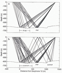
Knowing the three-dimensional locations of the reflectors, especially those seen in the daily records, is essential for a complete glaciological interpretation of any observed changes in them. The approximate longitudinal locations of the daily P-P, multiple P-P, and P-SV reflectors are shown in Figure 5, obtained by ray-tracing the first arrivals of each type of wave to each geophone. The bed was specified by RES (personal communication from T. Gades, 1994); RES data work well for this purpose because of their high spatial resolution. This migration is strictly valid only for reflectors located along this center-line profile.

Fig. 4.

Longitudinal cross-section using (a) horizontal and (b) vertical geophones. Superimposed lines represent the theoretical time–distance curves for various waves. Annotated lengths are one-way distances between a reflector and the shot-receiver axis at the ice surface. Note that axes limits differ between (a) and (b).

We can estimate the spatial extent of seismically observed changes at the bed by estimating the horizontal resolution of each geophone. Horizontal resolution is typically described in terms of the constructive interference that would occur if two reflections front nearby reflectors arrive at a geophone within one half-cycle of each other. For normal incidence, assuming a planar interface, all reflections of a spherical wavefront from within a circle of radius (λH/2)^1/2 should constructively interfere, where H is ice thickness. This circle defines the horizontal resolution (Reference Sheriff and GeldartSheriff and Geldart, 1995). In our case, λ in ice is about 45 m and H is about 450–600 m, yielding a radius of about 100–120 m. Thus, any subglacial layers that we observe seismically should be fairly continuous over an area of about 40 000 m² for each geophone. The sampled area for adjacent geophones will often have some overlap, but we might expect that a reflected wave arriving at each of the geophones along the 300 m long array would illuminate a region on the order of 200 m wide by 350 m long. The irregular bottom, however, may cause this illuminated area to be discontinuous, as described below.

Fig. 5.

First-arrival ray-tracing for daily-shot geometry. (a) P-P and P-SV rays. (b) The same rays with multiple P-P waves. The P-P reflector does not overlap with the others, suggesting that changes in P-P measurements may occur independently of P-SV or multiple P-P measurements.

Figure 5 indicates that the reflectors are distributed over a 1300 m length of the bed, and that the irregular bottom, combined with the large shot-receiver offset, results in reflectors for the different wave types that do not overlap. Therefore, comparisons of changes in P-P and multiple P-P reflections, for example, require caution because they represent different parts of the bed and the reflectors may be affected differently as subglacial conditions change. The P-P reflections come from a section of the bed about 650 m downstream of geophone 12. The P-SV and multiple P-P reflectors, unlike the P-P, are unevenly spaced compared to the surface spacing of the geophones, and they may lie on both the lee and stoss sides of bumps in the bed, as shown in Figure 5. Again, since such reflectors might be affected differently, two geophones 27 m apart on the surface may be recording changes within two independent subglacial regimes. As we will later show, the measurements of both P-SV and multiple P-P waves reveal that some of the reflectors were in fact topographically discontinuous and each region was affected differently.

Even though the shot, the geophone array and a reflector will typically lie within a single plane, that plane may not be vertical, requiring additional information from outside the plane to locate it. We determined the transverse position of the reflectors by comparing the radial distance of a reflector measured on the time–distance curves (Fig. 4) to a transverse cross-section of the study area measured by seismic reflections and RES (Fig. 6) at the approximate location of the P-P reflectors shown in Figure 5 (650 m down-glacier from geophone 12). The radius of each of the three semicircles in Figure 6 is equal to the distance from the shot-receiver axis to the three P-P reflectors N, C and S labeled in Figure 4; they are the loci of all possible locations for each of the reflectors (assuming travel through ice only). Note that the annotated distances are not depths; instead they are distances from the shot-receiver axis at the ice surface. Barring any unlikely englacial reflectors, reflection N (corresponding to a distance of 540 m) is unambiguously located about 350 m north of, and 100 m above, the deepest part of the bed (Fig. 6), at a depth of about 500 m. This lack of ambiguity is important as nearly all the morphological interpretations made in N&E rely on changes to P-P waves observed at this location.

Fig. 6.

Transverse cross-section of Black Rapids Glacier near 16 km. The vertical lines represent the borehole locations, purposefully selected to match seismic reflector locations used in this study. The semicircles represent the loci of the reflector locations for the P-P waves annotated in Figure 4. The dashed lines represent the most likely reflector locations for these waves.

The locations of the two other P-P reflectors, C and S, are more ambiguous because their loci have two intersections with the bed. From Snell’s law, we know that the tangent to each circle must be parallel to the transverse slope of the bed for a reflection to be recorded. Figure 6 shows the intersections that best meet this condition for reflectors C and S. This figure shows the significance of labeling these reflections N, C and S: north, center and south (or PP_N, PP_C and PP_S). Reflection PP_C comes from the center of the valley at a depth of about 600 m, and reflection PP_S probably comes from a point about 350 m south of the center line at a depth of 550 m. It is possible that one or both of these waves traveled through a subglacial layer that has a slower wave speed (e.g. till) for part of its path. In that case, the radius of its reflection locus would be decreased somewhat. On the other hand, if these reflections came from the top of a subglacial layer, other reflectors could be beneath; such reflections are impossible to identify confidently, yet they would contribute to the complex suite of P-P reflections shown in Figure 4.

The angles of incidence of these P-P reflections at the subglacial interface are important for later interpretation (N&E). Because of the large shot-receiver offsets and the measured ice thickness, we expect these angles to be about 45–50^°, which cannot be taken as “near-normal” incidence (i.e. near zero) in any analysis. To obtain a more accurate value for the angle of incidence for reflection PP_N, we utilize the move-out of its unobscured arrival times to calculate the slope of the basal interface relative to the surface following the migration procedures developed by Reference Clarke and EchelmeyerClarke and Echelmeyer (1996). This method shows that reflector PP_N was inclined upward about 2^°. This implies an angle of incidence of about 49–54^° for the rays reaching geophones 12–1, respectively. The incidence angles for reflection PP_C were estimated from ray tracing (Fig. 5), and were in the range 47–53^° across the geophone line. For PP_S, they were estimated to be 44–49^°.

The travel time of the brightest P-SV reflection (labeled in Fig. 4) corresponds to a distance of about 620 m from the shot-receiver axis, implying that this reflector is probably located near the deepest point of the cross-section, similar to reflector PP_C. An earlier, unlabeled P-SV reflection, with a 550 m distance, is probably situated along the northern valley wall at a location similar to PP_N in the cross-section. Again we note that these P-SV waves need not come from the same longitudinal position as the corresponding P-P returns, as shown in Figure 5a.

To summarize, our analysis shows that there are three prominent P-P reflections: the one labeled PP_N comes from the north side of the valley about 100 m above the deepest part of the channel (500 m depth); the one labeled PP_C comes from the near-deepest part of the channel (about 610 m) near its center line; and the one labeled PP_S comes from the south side at about 550 m depth. There are also relatively strong P-SV and multiple P-P reflections that probably come from the deepest part of the channel. It is the temporal changes in these reflections, particularly PP_N, that form the basis of our analysis of the basal morphology of Black Rapids Glacier in N&E.

Temporal Changes in Seismic Data

In undertaking these analyses, we found that there were two major categories of daily records, which we label “normal” and “anomalous”. Although there was some variation between the records within each category, the two categories are well distinguished. For most of the summer, the records were nearly identical, with only minor variations. The similarity in waveforms throughout the summer can be seen in Figure 7, which shows all of the daily traces for geophone 10H. Most of these traces show very few changes in amplitude or timing throughout the summer; these are the “normal” records. Only those associated with the drainage and motion events are “anomalous”; they occurred on days 165–167, 169–171 and 175. At first glance, the differences between these two record types are not large, but they are significant. We first describe the analysis methods, and then the distinguishing features of the normal and anomalous records.

Since neither the absolute timing (due to faulty triggers) nor the absolute amplitudes (due to variable source coupling) could be compared directly between traces, both of these values were then normalized using another wave in the same trace. However, it should be noted that source coupling was remarkably uniform throughout the study period, as can be seen in Figure 7, and this normalization was minimal. Quantitative comparisons of the changes in arrival time (e.g. Fig. 8a) and amplitude were then made. This was done with most combinations of the direct, reflected (P-P and P-SV) and multiple waves, realizing that normalizations using reflected waves are of questionable validity because their reflectors are at different locations.

Fig. 7.

Gather of traces from horizontal geophone 10 throughout summer. These are raw data with no amplitude modifications or filtering. For must of the summer, the measurements are nearly identical. Significant changes are apparent on days 169–171 and day 175.688. Also apparent, at the lower right, is the increase in ground roll speed due to decreasing snow thickness. Measurements on days 180 and 184 are different because the geophone was temporarily reoriented to measure SH waves.

Cross-correlating daily records was another effective way to quantitatively characterize their similarity. The set of daily traces at a given geophone was analyzed by comparing: (1) every trace with every other trace, (2) every trace with a single “typical” trace, (3) every trace with the average of all the traces at that geophone, or (4) each trace to the preceding trace. Different effects were illuminated by each method, but we found the fourth most useful. Figure 8b and c are examples of the fourth cross-correlation method: comparing each geophone’s recording to that of the preceding day. The mean correlation over all 12 geophones for each daily record is shown.

Digitally overlaying two records often proved to be the most useful technique for determining the nature and extent of the differences between them, particularly on days when large-scale changes occurred at the bed. On such days, comparisons of the amplitude of a particular wave had little value because it was often not clear if the same reflections were still being compared. Examples of such a comparison are shown in Figure 9.

Features of the Normal Records

There were no trends in arrival times for the various waves in the normal records. Figure 8a shows the difference in arrival time between the direct P-wave and the PP_N for all horizontal geophones, along with their mean for each seismogram (heavy circles). This pattern is typical of both vertical and horizontal geophones. The standard deviation of these means (not including the outliers) is about 2 ms, which is about the combined accuracy of our picking ability. The prominent outliers in this figure are associated with anomalous records. The apparent scatter of individual traces about the mean for a particular day is real: the move-outs of the direct and reflected P-waves are not the same, so each geophone records a slightly different time difference.

In general, there were few trends in the amplitudes of the various waves in the normal records. Those trends that we did identify were apparent only on the horizontal geophones; the vertical geophones showed almost no coherent changes. These include: (1) the P-P to P-SV amplitude ratio gradually decreased throughout the summer; (2) the ratio of P-P to multiple P-P increased after the second jökulhlaup (day 169), primarily due to a change in the multiple P-P; (3) the P-SV to multiple P-P amplitude ratio increased after day 169; and (4) in general, most of the amplitude ratios show more scatter after day 169. Here P-P refers to reflection N, P-SV to the 620 m P to SV reflection, and multiple P-P to the most prominent (630 m) P-P wave multiple. We might expect to find some variations as the geophones were displaced relative to the bed by glacier motion throughout the study period (a total of about 12 m), yet such changes are impossible to predict.

Fig. 8.

Examples of timing and cross-correlation analyses. (a) Plot of the difference in arrival times of direct P-wave and first P-P arrival: light circles are from individual traces and dark circle is the mean of all the traces. Several records are missing because the direct P-wave was not recorded. (b, c) Cross-correlations were made of each trace to the previously measured trace (e.g. trace 10 on day 158 to trace 10 on day 157), and the mean of these cross-correlations for all 12 traces for each seismogram is shown for the (a) horizontal and (b) vertical geophones. Although not resolved in (b), there are two data points on day 175, each with a correlation coefficient of about–0.05; no measurements were made using the vertical geophones on day 175.

We distinguished the effects of such daily motion from those related to changes in basal conditions using cross-correlations. By selecting one particular day as a standard for comparison (technique 2 in the previous subsection), we found that the greater the time interval between two records, the more dissimilar they were (that is, their correlation coefficient was reduced). This trend was linear with the number of days between the records, and thus was not related to temporal variations in basal conditions.

We eliminated the effects of this daily motion by comparing each trace to the previous one (technique 4 in the previous subsection), which highlights the difference between successive records. Results of this correlation over the study period for the vertical and horizontal geophones are shown in Figure 8b and c, respectively. Most of the records have a cross-correlation coefficient with the previous record of 0.75 or higher; these “nearly identical” records are the normal ones. There is somewhat more variation in the horizontal geophone records.

There are several “normal” records that have a cross-correlation coefficient less than 0.75, but extenuating circumstances apply in each of these cases. For example, records from days 144 and 146 have a poor ice–shot coupling, and all waves, including the direct P-wave and ground roll, are of a lower amplitude, as can be seen in Figure 7. This lower amplitude causes slight differences in waveforms, and thus a weaker correlation. Measurements made on days 180 and 184 have low coefficients because several of the geophones on each geophone cable were temporarily switched or reoriented to study local effects, causing some traces to be inverted (Fig. 7). Inspection of these records using overlays reveals that they too are “normal” once these experimental discrepancies are accounted for.

Overlays of two such normal records highlight their similarity (Fig. 9a). The cross-correlation between the two records overlaid in this figure was about 0.9. No amplitude scaling was applied; this shows that the source/ice coupling was nearly equal for the two records, as was typical throughout the summer. The measurement on day 159 is missing several of the direct waves because of an error in timing.

Features of the Anomalous Records

There were only three periods throughout the summer when significant changes in the seismic reflections were observed. We refer to these as anomalies I–III; each corresponds to one of the three lake-drainage events. Unfortunately, no longitudinal cross-sections were made during these events and therefore none could be used to constrain their longitudinal extent.

Anomaly I

There were several changes associated with the first jökulhlaup, on days 165–167. In Figure 9b, which compares day 166 (anomalous) to day 159 (normal), reflection PP_N was unaffected (Figs 7 and 9b), but there were minor changes to PP_C and larger changes to PP_S, particularly on the horizontal geophones. The latter appears to have changed polarity, but this finding is somewhat ambiguous.

The early multiple (corresponding to a distance of 620 m from the shot-receiver axis, immediately preceding the time–distance curve labeled “P-P P-P: 630 m” in Figure 9b) also appears to have changed polarity following the first drainage event. The later multiple appears only slightly shifted, with perhaps a minor increase in amplitude. The changes in these multiples were smaller on the horizontal geophones, partly due, perhaps, to the fact that these P-waves were much clearer on the vertical geophones. Minor changes were observed on the horizontal geophones for the 620 m P-SV wave.

Anomalies II and III

Seismic anomalies were observed following the second and third jökulhlaups as well. The changes from the normal records were more prominent than those observed during anomaly I. It appears that each of the three P-P reflectors was affected, as well as the multiple P-P and P-SV waves; these reflectors span the entire 700 m by 1300 m study area (Figs 5 and 6). These anomalies, on days 169–171 and then on day 175, were nearly identical despite being separated by normal records on days 173 and 174 (Fig. 9c–e), so we discuss their changes together. Two measurements were made using the horizontal geophones during the early part of the third lake-draining event: the first was anomalous and the second, 36 min later, was completely back to normal (days 175.688 and 175.713, respectively, in Figure 7). There are several interesting features of these anomalous records, and it is these anomalous features that give us the most definitive constraints on the changing morphology of the basal interface.

Fig. 9.

(a) Overlay comparison of two normal seismograms (days 158 (heavy) and 159) which have a cross-correlation coefficient greater than 0.9 and are typical of most of the measurements throughout the summer. (b) Overlay comparison of anomaly I (day 166, heavy) to a normal day (day 158, as in (a)). Several changes are apparent in the later-arriving P-P waves and in the P-P multiple arrival immediately preceding 630 m multiple. (c) Overlay comparison of anomaly II (day 171, heavy) to a normal day (day 159), using horizontal geophones. Major changes are apparent in almost all of the waves. Horizontal and vertical geophones did not change identically during this anomaly (e.g. slight changes are apparent on the 630 m P-S wave on the horizontal geophones, but much larger changes are observed on some of the vertical geophones). (d) Overlay comparison of anomaly II (heavy) to a normal day, using vertical geophones, from the same days as in (c). (Continued...)

The first P-P arrival on those anomalous records was about 10 ms later than normal (Figs 7, 8a and 9c; no data points exist for days 170 and 175.688 in Figure 8a because no direct P-wave was recorded due to timing errors.) This first P-P arrival no longer originates from reflector N. If it did, the 10 ms increase would require either that the ice thickened by over 17 m in one day or that the bulk-ice wave speed temporarily dropped by almost 150 m s^-1, while the near-surface wave speed remained constant. Neither scenario is plausible, especially given the 36 min time constraint. This new first arrival may be from a new reflector, the second arrival in the normal records, and/or from the bottom of a basal layer beneath reflector N. These possibilities are considered in N&E.

Most of the subsequent reflections during anomalies II and III are also uncharacteristic of the normal records. Several of the P-P waves seem to be phase-reversed from those on the normal records, and they have changed in roughly the same manner on both the vertical and horizontal geophones. Of all the P-P waves, reflection PP_C, from near the deepest part of the valley, appears to have changed the least.

Fig. 9.

(e) Overlay comparison of anomaly III to anomaly II. The only seismogram from anomaly III, recorded by the horizontal geophones on day 175.688 (dark), is compared to the same anomaly II seismogram (day 171) shown in (c). Although the direct P-waves were truncated due to timing errors and several traces were noisy due to melted-out geophones, it is dear that the remaining measurements on day 175.688 are nearly identical to those of day 171. Superimposed on all of the overlays are travel-time curves of various waves along with their one-way distance from the shot-receiver axis to the reflector, as annotated.

The change in the P-SV waves is different on the two orientations of geophones. On both, the first peak of the earlier P-SV wave (corresponding to about 550 m distance from the shot-receiver axis) decreases to near zero amplitude, and the next peak may be phase-reversed. The second P-SV wave (620 m distance) remains essentially unchanged in amplitude or phase on the horizontal geophones, while it is somewhat phase-shifted on the vertical geophones. These two waves display complex structure. For example, the shape of the anomalous 620 m P-SV wave (Fig. 9c) sometimes has two peaks without an intervening trough. This effect can only be caused through superposition of more than one wave; interpretation of such changes would be ambiguous. The changes to both P-SV waves are more pronounced on the geophones closest to the shot, suggesting that the reflectors for different geophone arrivals are located in different subglacial regimes along the bed. This possibility is also suggested by Figure 5.

Significant changes were also observed in the P-P multiple waves. On both the horizontal and vertical geophones, the later-arriving, more prominent multiple appears to have changed polarity and possibly increased in amplitude. The earlier multiple does not seem to have changed significantly on the vertical geophones. Changes in polarity and amplitude are apparent on the horizontal geophones with offsets of 1450–1650 m, bin not on the closer ones. As with the P-SV waves, this suggests that this multiple results from discontinuous reflectors that are affected independently.

There are only minor differences between the anomalous records from days 169–171 (event II) and day 175.688, as is shown in Figure 9e and the cross-correlations in Figure 8b and e. The anomalous record from day 175 in Figure 9e is missing the direct P-wave arrival because of timing errors, but it has been shifted properly and is nearly identical to the anomalous records from the previous event. Each of the reflections returned to normal after events II and III, except for the 620 m P-SV wave, which continued to have a slight phase shift during the interval between the two events. That these two anomalous records are separated in time by three normal daily records and yet are nearly identical indicates that the basal conditions existing after the second and third jökulhlaups, which came from different lakes, were similar over much of the bed and that the changes are the result of similar processes.

It is significant that the seismic records during event I were only slightly changed from normal ones, while those during events II and III were markedly different, especially given the magnitude and timing of the associated glacier motion events, as is discussed in the following section.

Correlation of Drainage, Survey and Seismic Measuments

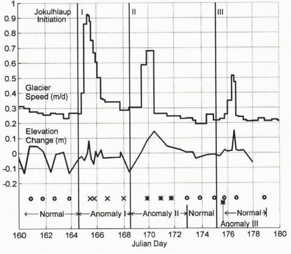
The sequence of drainage events, seismic anomalies, increased motion, and surface-elevation change is shown in Figure 10. This figure allows us to constrain the duration of the seismic anomalies, assuming that no changes occurred between our measurements. As we will discuss, this assumption should be regarded with caution. We use the initiation of the jökulhlaups as a minimum estimate for the initial time of a seismic anomaly.

Fig. 10.

Correlation of jökulhlaups, increases in ice motion, surface-elevation change and seismic anomalies. Estimated initiation times of jökulhlaups are represented by thin vertical lines with Roman numerals corresponding to those in Figures 1 and 2. Circles at bottom represent “normal” seismic measurements. Crosses and asterisks represent the two types of anomalous seismic measurements.

The initiation of each jökulhlaup can be estimated fairly accurately. In the early afternoon of day 164 we observed water from the first lake draining through a channel cut into its bank. This muddy water traveled down-glacier along the ice surface, filling several small lakes bordering the moraine of a tributary glacier, before entering a moulin. We estimate that the water first reached the bed by day 164.6 ± 0.1 d, at the latest. The second jökulhlaup was not observed, but we did find a freshly drained supraglacial pothole 1 day later; automated camera data indicate that several such potholes may have drained simultaneously (personal communication from W. Reference Raymond, Benedict, Harrison, Echelmeyer and SturmHarrison, 1995). Our survey data show that increased motion associated with this jökulhlaup began as early as day 168.5 and certainly by day 169.3. We closely observed the third jökulhlaup, which emptied water directly into a tunnel at the lake bottom, and estimate drainage onset at day 175.1 ± 0.2 days. These estimates are shown in Figure 10 as vertical lines.

All of the seismic records measured during the 3 days of the first drainage event showed some variation from normal (shown with a cross in Figure 10). Although the next lake-drainage event occurred before the records returned to normal, we assume that this first anomaly was reversible since records following anomalies II and III were back to normal. Thus, we estimate the minimum duration of anomaly I as the time between the first anomalous record and the last record before the second jökulhlaup (2.1 days), and the maximum duration as the time between the initiation of the first and second jökulhlaups (3.9 days) (Fig. 10). The last anomalous record during event I was obtained at least 1 day after the period of increased basal motion had ended (Fig. 10).

Several seismic records obtained after the second jökulhlaup began were anomalous (asterisk in Fig. 10); they were followed by normal records until the initiation of the third event. We estimate the minimum duration of this second anomaly as the interval between anomalous measurements (1.9 days), and the maximum duration from the initiation of draining to the next normal record (4.4 days). Our first anomalous seismic measurement during this event occurred after the increase in motion began, but we continued to record anomalous measurements for another full day after the glacier speed returned to the pre-drainage magnitude (Fig. 10).

The third seismic anomaly was recorded during the early stages of the third jökulhlaup, but ended before the increase in basal motion began (Fig. 10). We have only one seismic record during this anomaly (asterisk in Fig. 10 on day 175.688); and we therefore estimate its maximum duration as beginning at drainage initiation and extending to the next normal record (0.6 days). If we assume this anomaly began immediately prior to its measurement and ended immediately prior to the next (normal) measurement; the actual duration could be as little as 36 min. However, as the record following the anomalous one was completely back to the normal state with no hysteresis, it seems possible that the transitions between states could lake even less than 30 min.

That we have unequivocal measurements of transitions occurring over about 1 km² of the bed in less than 36 min is an unexpected result. It indicates that our daily seismic sampling interval was too coarse to measure all the potential changes that may have occurred and that, at least following jökulhlaups, this interval could justifiably be decreased to 15 min during jökulhlaups.

The number of processes that can affect such a large area so quickly and reversibly is limited, and these timing constraints are important for interpretation in terms of basal morphology (N&E). A further constraint to be considered is that, while the lake drainages appear to have caused both the seismic anomalies and the increased motion, the two effects may result from different processes as they often do not strictly overlap, as shown in Figure 10.

Conclusions

We have conclusively demonstrated the feasibility of an active seismic technique to measure temporal variations in the bed of a glacier that relate to variations in basal motion. After recording seismic reflections from the bed of Black Rapids Glacier for a period of 45 days in spring 1993, we found that the only measurements which showed significant variation were immediately following jökulhlaups that also caused increased glacier motion. While these particular motion events were small and short-lived, these methods could easily be adapted to investigate the changing sub-glacial conditions that relate to why glaciers surge or form ice streams. The spatial scale of these reflectors is much larger than that sampled by individual boreholes. It should also he noted that changing surface conditions, such as the amount of meltwater present or small amounts of normal glacier motion, do not affect the seismic reflection data.

We learned several new results regarding the basal dynamics of Black Rapids Glacier. Two of the seismic anomalies were identical despite being caused by jökulhlaups from different locations. In both cases, the anomalous measurements returned to nearly pre-anomalous forms within 2 days or less. Therefore the responsible mechanism is not only independent of the origin of the basal water input but also causes no permanent change to the bed’s seismic character. This mechanism must also be able to act over the same 1 km² area of the bed in less than 36 min. And because the timing between the seismic anomalies and the increased basal motion varied with each event, we know that, while they were both caused by jökulhlaups, the temporal correlation between the two is not one-to-one.

The most important specific changes in the seismic records were:

• (i) The First P-P reflection disappeared during two of the events, then returned to normal each time. This reflection comes from a location which is about 100 m above the deepest part and on the north side of the glacier valley (PP_N in Fig. 6).

• (ii) The P-P reflection that comes from the deepest part of the valley cross-section (PP_C in Fig. 6) showed the least change of any reflection.

• (iii) The P-SV reflection coming from a location near P-P reflector PP_N decreased in amplitude to near zero during the second two anomalies. The P-SV reflection from the deepest part of the valley (near PP<_C in Fig. 6) did not show strong changes on the horizontal geo-phones, but it did on the vertical ones.

• (iv) During the second two anomalies the 630 m P-P wave multiple (most likely from the deepest part of the valley cross-section) showed clear phase reversals.

These results impose stringent constraints on the changing properties of the bed. In our second paper in this issue (N&E) we investigate what changes in basal morphology can lead to these observed seismic changes.