1 Introduction
Bubble dynamics is a classical field associated with wide and important applications in science and technology (Young Reference Young1989; Leighton Reference Leighton1994; Brennen Reference Brennen2013). Its study was started in 1917 by Lord Rayleigh during his work with the Royal Navy to investigate cavitation damage on ship propellers. Over several decades his work was refined and developed by Plesset, Prosperetti and others (Plesset & Prosperetti Reference Plesset and Prosperetti1977; Tomita & Shima Reference Tomita and Shima1977; Vokurka Reference Vokurka1986; Feng & Leal Reference Feng and Leal1997; Prosperetti Reference Prosperetti2004; Zhang & Li Reference Zhang and Li2012). The resulting equation, known as the Rayleigh–Plesset equation, models the oscillations of a gas-filled spherical cavity in an infinite incompressible liquid. Gilmore (Reference Gilmore1952) was the first to incorporate sound radiation into the liquid from the oscillating bubble. Keller & Miksis (Reference Keller and Miksis1980) also incorporated sound radiation from the oscillating bubble, leading to a more popular model, the Keller–Miksis equation.
Both the Rayleigh–Plesset equation and the Keller–Miksis equation are nonlinear and therefore are often analysed numerically (see, for example, Lauterborn & Kurz Reference Lauterborn and Kurz2010). However, in recent years, approximate analytical solutions have been sought to these equations, since analytical analysis is a powerful tool for improved understanding of the qualitative behaviour and trends of phenomena.
Obreschkow, Bruderer & Farhat (Reference Obreschkow, Bruderer and Farhat2012) derived accurate explicit analytical approximate solutions of the Rayleigh equation for the collapse of an empty spherical bubble. Amore & Fernández (Reference Amore and Fernández2013) developed a rigorous justification and explanation for the remarkable accuracy of these approximations. Kudryashov & Sinelshchikov (Reference Kudryashov and Sinelshchikov2014) found an implicit analytical solution to the Rayleigh equation for an empty bubble (in terms of the hypergeometric function) and for a gas-filled bubble (in terms of the Weierstrass elliptic function). Mancas & Rosu (Reference Mancas and Rosu2016) obtained the parametric rational Weierstrass periodic solutions using the connection between the Rayleigh–Plesset equation and Abel’s equation. Van Gorder (Reference Van Gorder2016) made a theoretical study for
 $N$
-dimensional bubbles with arbitrary polytropic index of the bubble gas.
Both viscous and compressible effects are neglected in the above theoretical studies. However the viscous effects are significant for microbubbles (Smith & Wang Reference Smith and Wang2017) and the compressible effects are essential for inertial collapse of bubbles (Leighton Reference Leighton1994; Lauterborn & Kurz Reference Lauterborn and Kurz2010). Compressible effects were studied by Shapiro & Weinstein (Reference Shapiro and Weinstein2011) and Costin, Tanveer & Weinstein (Reference Costin, Tanveer and Weinstein2013), in the linearized approximation. In particular, they proved that the amplitude of bubble oscillation decays exponentially, in the form
 $\text{e}^{-\unicode[STIX]{x1D6E4}t}$
,
 $\unicode[STIX]{x1D6E4}>0$
, as time advances. Furthermore the decay rate parameter
 $\unicode[STIX]{x1D6E4}$
was derived in terms of the Mach number and the Weber number.
We will study bubble oscillation at large amplitude with significant nonlinear compressible effects, which is associated with the loss of energy of a bubble system due to acoustic radiation to the far field (Prosperetti & Lezzi Reference Prosperetti and Lezzi1986; Lezzi & Prosperetti Reference Lezzi and Prosperetti1987; Fuster, Dopazo & Hauke Reference Fuster, Dopazo and Hauke2011; Wang Reference Wang2013, Reference Wang2016). We will investigate the decay of large-amplitude bubble oscillation, to evaluate the time histories of the energy, frequency and maximum and minimum radii of an oscillating bubble. Inertial bubble dynamics is associated with important applications such as cavitation damage to pumps, turbines and propellers (Young Reference Young1989; Duncan & Zhang Reference Duncan and Zhang1991; Zhang, Duncan, & Chahine Reference Zhang, Duncan and Chahine1993; Brennen Reference Brennen2013) and underwater explosions (Wang Reference Wang2013; Zhang et al. Reference Zhang, Cui, Cui and Wang2015). Ultrasound-driven microbubbles are widely used in biomedical technology (Klaseboer et al. Reference Klaseboer, Fong, Turangan, Khoo, Szeri, Calvisi, Sankin and Zhong2007; Wang & Blake Reference Wang and Blake2010, Reference Wang and Blake2011; Wang & Manmi Reference Wang and Manmi2014; Wang, Manmi & Liu Reference Wang, Manmi and Liu2015), sonochemistry (Suslick & Crum Reference Suslick, Crum and Crocker1997) and ultrasonic cavitation cleaning (Ohl et al. Reference Ohl, Arora, Ikink, de Jong, Versluis, Delius and Lohse2006).
Compressible bubble dynamics can be described approximately by a short time scale associated with inertial oscillation and a long time scale associated with acoustic radiation damping, and is thus analysed using the multi-scaled perturbation method of Kuzmak (Reference Kuzmak1959) and Luke (Reference Luke1966), which was developed for studying nonlinear oscillations and the nonlinear dispersive wave problems. This asymptotic method has successfully determined the decay rate of large-amplitude oscillations of an incompressible viscous drop (Smith Reference Smith2010), a generalization of the Landau equation for travelling waves in two-dimensional plane Poiseuille flow (Smith & Wissink Reference Smith and Wissink2015) and necessary conditions for the invariant manifold of the turbulent attractor in two-dimensional Kolmogorov flow (Smith & Wissink Reference Smith and Wissink2017). It is particularly suitable for the multi-scaled nonlinear oscillations which occur in fluid mechanics.
The remainder of the paper is organized as follows. The mathematical model for the radiative decay of bubble oscillations is described in § 2. In § 3, the Keller–Miksis equation is analysed using a multi-scaled method with a short time scale associated with inertial oscillation and a long time scale with radiation damping. The leading-order problem is solved analytically on the inertial oscillation time scale. In § 4, the analytical solutions are firstly compared with the numerical solutions of the Keller–Miksis equation and experimental observations. A parametric analysis is then carried out with the above theory for the energy of the bubble system, frequency and amplitude of oscillation in terms of the dimensionless initial pressure of the bubble gases, Weber number and polytropic index of the bubble gas. Finally, in § 5, this study is summarized and the key outcomes are identified.
2 Mathematical model
We study the Keller–Miksis equation for a spherical gas bubble in a compressible liquid under adiabatic conditions
 $$\begin{eqnarray}\left(1-\frac{1}{c}\frac{\text{d}\bar{R}}{\text{d}\bar{t}}\right)\bar{R}\frac{\text{d}^{2}\bar{R}}{\text{d}\bar{t}^{2}}+\frac{3}{2}\left(\frac{\text{d}\bar{R}}{\text{d}\bar{t}}\right)^{2}\left(1-\frac{1}{3c}\frac{\text{d}\bar{R}}{\text{d}\bar{t}}\right)=\left(1+\frac{1}{c}\frac{\text{d}\bar{R}}{\text{d}\bar{t}}\right)\frac{\bar{p}_{l}}{\unicode[STIX]{x1D70C}}+\frac{\bar{R}}{\unicode[STIX]{x1D70C}c}\frac{\text{d}\bar{p}_{l}}{\text{d}\bar{t}},\end{eqnarray}$$
in which
 $\bar{p}_{l}$
is the pressure of liquid at the bubble surface and given as follows
 $$\begin{eqnarray}\bar{p}_{l}=\bar{p}_{g0}\left(\frac{\bar{R}_{max}}{\bar{R}}\right)^{3\unicode[STIX]{x1D705}}-\frac{2\unicode[STIX]{x1D70E}}{\bar{R}}-(\bar{p}_{\infty }-\bar{p}_{v})-\frac{4\unicode[STIX]{x1D707}}{\bar{R}}\frac{\text{d}\bar{R}}{\text{d}\bar{t}},\end{eqnarray}$$
where
 $\bar{R}(\bar{t})$
is the spherical bubble radius at time
 $\bar{t}$
,
 $c$
is the speed of sound in the liquid,
 $\bar{R}_{max}$
the initial maximum bubble radius,
 $\unicode[STIX]{x1D70C}$
the liquid density,
 $\bar{p}_{\infty }$
the hydrostatic pressure of the liquid,
 $\bar{p}_{v}$
the vapour pressure of the liquid,
 $\bar{p}_{g0}$
the initial pressure of the bubble gases,
 $\unicode[STIX]{x1D705}>1$
the polytropic index,
 $\unicode[STIX]{x1D70E}$
the surface tension and
 $\unicode[STIX]{x1D707}$
the liquid viscosity.
The Keller–Miksis equation (2.1) is well established and its advantages and limitations have been widely discussed in the literature. Among the limitations, it is well known that it has problems capturing all the damping mechanisms occurring during the collapse, which is translated into an over-estimation of the amplitude of the rebound intensity for very intense collapses.
Equation (2.1) is scaled using
 $\bar{R}=\bar{R}_{max}R$
and
 $\bar{t}=\bar{R}_{max}t/U$
, where
 $$\begin{eqnarray}\unicode[STIX]{x1D6E5}=\bar{p}_{\infty }-\bar{p}_{v},\quad U=\sqrt{\frac{\unicode[STIX]{x1D6E5}}{\unicode[STIX]{x1D70C}}},\end{eqnarray}$$
in which
 $\unicode[STIX]{x1D6E5}$
is the characteristic pressure of the liquid and
 $U$
is a reference velocity. The dimensionless Keller–Miksis equation takes the form
 $$\begin{eqnarray}\left(1-\unicode[STIX]{x1D716}\frac{\text{d}R}{\text{d}t}\right)R\frac{\text{d}^{2}R}{\text{d}t^{2}}+\frac{3}{2}\left(\frac{\text{d}R}{\text{d}t}\right)^{2}\left(1-\frac{\unicode[STIX]{x1D716}}{3}\frac{\text{d}R}{\text{d}t}\right)=\left(1+\unicode[STIX]{x1D716}\frac{\text{d}R}{\text{d}t}\right)p_{l}+\unicode[STIX]{x1D716}R\frac{\text{d}p_{l}}{\text{d}t},\end{eqnarray}$$
in which
 $$\begin{eqnarray}p_{l}=\frac{p_{g0}}{R^{3\unicode[STIX]{x1D705}}}-\frac{2}{WeR}-1-\frac{4}{ReR}\frac{\text{d}R}{\text{d}t},\end{eqnarray}$$
where
 $$\begin{eqnarray}Re=\frac{\unicode[STIX]{x1D70C}U\bar{R}_{max}}{\unicode[STIX]{x1D707}},\quad We=\frac{\bar{R}_{max}\unicode[STIX]{x1D6E5}}{\unicode[STIX]{x1D70E}},\quad p_{g0}=\frac{\bar{p}_{g0}}{\unicode[STIX]{x1D6E5}}<1,\quad \unicode[STIX]{x1D716}=\frac{U}{c}\end{eqnarray}$$
are the large Reynolds number, the Weber number, the dimensionless initial pressure of the bubble gases and the small Mach number, respectively. For convenience, we choose the initial time at the maximum bubble radius
 $\bar{R}_{max}$
. The initial conditions are
 $$\begin{eqnarray}R(0)=1,\quad \frac{\text{d}R}{\text{d}t}(0)=0.\end{eqnarray}$$
With the choice of the maximum radius
 $\bar{R}_{max}$
as the reference length, the initial conditions become (2.7). The essential independent dimensionless parameters for the system are limited to four parameters: the Mach number
 $\unicode[STIX]{x1D716}$
, the dimensionless minimum pressure
 $p_{g0}$
of the bubble at the maximum radius during the first cycle, the polytropic index
 $\unicode[STIX]{x1D705}$
of the bubble gas and the Weber number
 $We$
. The analysis is thus simplified using this combination of the initial conditions and dimensionless parameters.
The dimensionless equilibrium radius
 $R_{eq}$
is defined by
 $R_{eq}=\bar{R}_{eq}/\bar{R}_{max}$
, where
 $\bar{R}_{eq}$
is the dimensional equilibrium radius which is more easily measured in experiments than the dimensionless initial pressure of the bubble gases
 $p_{g0}$
. These quantities are linked via the equation
 $$\begin{eqnarray}p_{g0}=R_{eq}^{3\unicode[STIX]{x1D705}}\left\{1+\frac{2}{WeR_{eq}}\right\}.\end{eqnarray}$$
After multiplying by
 $2R^{2}\,\text{d}R/\text{d}t$
, equation (2.4) can be rewritten in the form
 $$\begin{eqnarray}\frac{\text{d}E}{\text{d}t}=R^{2}\frac{\text{d}R}{\text{d}t}\left[\unicode[STIX]{x1D716}F-\frac{4}{ReR}\frac{\text{d}R}{\text{d}t}+O\!\left(\frac{\unicode[STIX]{x1D716}}{Re}\right)\right],\end{eqnarray}$$
in which
 $$\begin{eqnarray}F=R\frac{\text{d}R}{\text{d}t}\frac{\text{d}^{2}R}{\text{d}t^{2}}+\frac{1}{2}\left(\frac{\text{d}R}{\text{d}t}\right)^{3}+\frac{\text{d}R}{\text{d}t}\left(\frac{p_{g0}}{R^{3\unicode[STIX]{x1D705}}}-\frac{2}{WeR}-1\right)+R\frac{\text{d}}{\text{d}t}\left(\frac{p_{g0}}{R^{3\unicode[STIX]{x1D705}}}-\frac{2}{WeR}\right),\end{eqnarray}$$
where the energy of a bubble system
 $E(t)$
is defined as follows
 $$\begin{eqnarray}E(t)=\frac{1}{2}R^{3}\left(\frac{\text{d}R}{\text{d}t}\right)^{2}+\frac{p_{g0}}{3(\unicode[STIX]{x1D705}-1)}R^{-3(\unicode[STIX]{x1D705}-1)}+\frac{1}{3}R^{3}+\frac{R^{2}}{We}.\end{eqnarray}$$
The first term on the right-hand side of (2.11) is associated with the kinetic energy of the surrounding liquid, the second and third terms the potential energy of the bubble gas and the last term the potential energy associated with surface tension at the interface. The kinetic energy of the gas is negligible since the density of gases is usually three orders of magnitude smaller than that of liquids. The initial condition for energy is
 $$\begin{eqnarray}E(0)=\frac{p_{g0}}{3(\unicode[STIX]{x1D705}-1)}+\frac{1}{3}+\frac{1}{We}.\end{eqnarray}$$
Henceforth, we assume that
 $1/Re\ll \unicode[STIX]{x1D716}\ll 1$
, so that compressibility effects dominate viscous effects.
3 Strongly nonlinear analysis
The damped oscillations of a bubble in a compressible Newtonian fluid are modelled using two time scales. The bubble radius
 $R$
varies significantly over a time scale corresponding to the period
 $2\unicode[STIX]{x03C0}/\unicode[STIX]{x1D714}$
of inertial oscillation, where the (angular) frequency is
 $\unicode[STIX]{x1D714}$
. The period (or frequency) and the minimum/maximum bubble radii change on a time scale of the order of the reciprocal of the Mach number
 $1/\unicode[STIX]{x1D716}$
associated with compressibility. We therefore introduce two time variables
 $t_{i}$
and
 $t_{c}$
associated with the inertial and compressible time scales (Kuzmak Reference Kuzmak1959; Kevorkian & Cole Reference Kevorkian and Cole1981; Smith Reference Smith2005), respectively,
 $$\begin{eqnarray}\displaystyle & \displaystyle \frac{\text{d}t_{i}}{\text{d}t}=\unicode[STIX]{x1D714}, & \displaystyle\end{eqnarray}$$
 $$\begin{eqnarray}\displaystyle & \displaystyle t_{c}=\unicode[STIX]{x1D716}t, & \displaystyle\end{eqnarray}$$
 $$\begin{eqnarray}\displaystyle & \displaystyle \frac{\text{d}}{\text{d}t}=\unicode[STIX]{x1D714}\frac{\unicode[STIX]{x2202}}{\unicode[STIX]{x2202}t_{i}}+\unicode[STIX]{x1D716}\frac{\unicode[STIX]{x2202}}{\unicode[STIX]{x2202}t_{c}}, & \displaystyle\end{eqnarray}$$
 $\unicode[STIX]{x1D714}$
needs to be chosen so that, in terms of
 $t_{i}$
, the period of oscillation of the leading-order solution is independent of
 $t_{c}$
. The period on this
 $t_{i}$
scale is then an arbitrary constant which we specify to be
 $2\unicode[STIX]{x03C0}$
without loss of generality. In other words, the leading-order solution is periodic in
 $t_{i}$
, with period precisely
 $2\unicode[STIX]{x03C0}$
, so that the changes in the frequency of the original problem are accounted for by determining a separate equation for
 $\unicode[STIX]{x1D714}$
below.
Using (3.1c ), the Keller–Miksis equation (2.4) becomes
 $$\begin{eqnarray}\displaystyle & & \displaystyle R\left(\unicode[STIX]{x1D714}^{2}\frac{\unicode[STIX]{x2202}^{2}R}{\unicode[STIX]{x2202}t_{i}^{2}}+2\unicode[STIX]{x1D716}\unicode[STIX]{x1D714}\frac{\unicode[STIX]{x2202}^{2}R}{\unicode[STIX]{x2202}t_{i}\unicode[STIX]{x2202}t_{c}}+\unicode[STIX]{x1D716}\frac{\text{d}\unicode[STIX]{x1D714}}{\text{d}t_{c}}\frac{\unicode[STIX]{x2202}R}{\unicode[STIX]{x2202}t_{i}}+\unicode[STIX]{x1D716}^{2}\frac{\unicode[STIX]{x2202}^{2}R}{\unicode[STIX]{x2202}t_{c}^{2}}\right)+\frac{3}{2}\left(\unicode[STIX]{x1D714}\frac{\unicode[STIX]{x2202}R}{\unicode[STIX]{x2202}t_{i}}+\unicode[STIX]{x1D716}\frac{\unicode[STIX]{x2202}R}{\unicode[STIX]{x2202}t_{c}}\right)^{2}\nonumber\\ \displaystyle & & \displaystyle \quad =\frac{p_{g0}}{R^{3\unicode[STIX]{x1D705}}}-\frac{2}{WeR}-1+\unicode[STIX]{x1D716}F-\frac{4\unicode[STIX]{x1D714}}{ReR}\frac{\unicode[STIX]{x2202}R}{\unicode[STIX]{x2202}t_{i}}+O\left(\frac{\unicode[STIX]{x1D716}}{Re}\right).\end{eqnarray}$$
We introduce an expansion for the bubble radius of the form
 $$\begin{eqnarray}R\sim R_{0}(t_{i},t_{c})+\unicode[STIX]{x1D716}R_{1}(t_{i},t_{c}),\quad F\sim F_{0}(t_{i},t_{c}),\end{eqnarray}$$
as
 $\unicode[STIX]{x1D716}\rightarrow 0$
. At leading order in (3.2) we obtain
 $$\begin{eqnarray}\unicode[STIX]{x1D714}^{2}R_{0}\frac{\unicode[STIX]{x2202}^{2}R_{0}}{\unicode[STIX]{x2202}t_{i}^{2}}+\frac{3}{2}\unicode[STIX]{x1D714}^{2}\left(\frac{\unicode[STIX]{x2202}R_{0}}{\unicode[STIX]{x2202}t_{i}}\right)^{2}=\frac{p_{g0}}{R_{0}^{3\unicode[STIX]{x1D705}}}-\frac{2}{WeR_{0}}-1.\end{eqnarray}$$
We also introduce an expansion for the energy of the bubble system of the form
 $$\begin{eqnarray}E\sim E_{0}(t_{c})+\unicode[STIX]{x1D716}E_{1}(t_{i},t_{c}),\end{eqnarray}$$
where the dependence of
 $E_{0}$
only on
 $t_{c}$
and
 $$\begin{eqnarray}E_{0}(t_{c})=\frac{1}{2}\unicode[STIX]{x1D714}^{2}R_{0}^{3}\left(\frac{\unicode[STIX]{x2202}R_{0}}{\unicode[STIX]{x2202}t_{i}}\right)^{2}+\frac{p_{g0}R_{0}^{-3(\unicode[STIX]{x1D705}-1)}}{3(\unicode[STIX]{x1D705}-1)}+\frac{R_{0}^{3}}{3}+\frac{R_{0}^{2}}{We}\end{eqnarray}$$
follow from (2.9) and (2.11), respectively. The energy of a transient bubble system decreases during a very short period of time at the end of the collapse due to acoustic radiation (Wang Reference Wang2016). In the present approach, we consider the loss of the average energy for each cycle of oscillation rather than the transient time history of the energy during that cycle. It is shown in (3.5) that the average energy of a bubble system changes on the long compressible time scale of the order
 $1/\unicode[STIX]{x1D716}$
. We also show subsequently that the period of the oscillation, maximum and minimum bubble radii all change on the long compressible time scale of the order
 $1/\unicode[STIX]{x1D716}$
.
Equation (3.4) is readily integrated to yield
 $$\begin{eqnarray}Q^{2}=\unicode[STIX]{x1D714}^{2}\left(\frac{\unicode[STIX]{x2202}R_{0}}{\unicode[STIX]{x2202}t_{i}}\right)^{2}=\frac{1}{R_{0}^{3}}\left\{-\frac{2p_{g0}R_{0}^{-3(\unicode[STIX]{x1D705}-1)}}{3(\unicode[STIX]{x1D705}-1)}-\frac{2R_{0}^{2}}{We}-\frac{2R_{0}^{3}}{3}+2E_{0}(t_{c})\right\},\end{eqnarray}$$
where
 $$\begin{eqnarray}Q=\unicode[STIX]{x1D714}\frac{\unicode[STIX]{x2202}R_{0}}{\unicode[STIX]{x2202}t_{i}}=\pm \sqrt{\frac{1}{R_{0}^{3}}\left\{-\frac{2p_{g0}R_{0}^{-3(\unicode[STIX]{x1D705}-1)}}{3(\unicode[STIX]{x1D705}-1)}-\frac{2R_{0}^{2}}{We}-\frac{2R_{0}^{3}}{3}+2E_{0}(t_{c})\right\}}.\end{eqnarray}$$
The collapse stage from the maximum bubble radius to the minimum bubble radius corresponds to the negative sign and the expansion stage from the minimum bubble radius to the maximum bubble radius corresponds to the positive sign.
An oscillating bubble attains its maximum or minimum when
 $\unicode[STIX]{x2202}R_{0}/\unicode[STIX]{x2202}t_{i}=0$
. Using (3.7), the maximum radius
 $R_{max}(E_{0},p_{g0},\unicode[STIX]{x1D705},We)$
and the minimum bubble radius
 $R_{min}(E_{0},p_{g0},\unicode[STIX]{x1D705},We)$
are defined to be two successive roots of
 $$\begin{eqnarray}g(R_{0},E_{0},p_{g0},\unicode[STIX]{x1D705},We)\equiv -\frac{2p_{g0}R_{0}^{-3(\unicode[STIX]{x1D705}-1)}}{3(\unicode[STIX]{x1D705}-1)}-\frac{2R_{0}^{2}}{We}-\frac{2R_{0}^{3}}{3}+2E_{0}=0\end{eqnarray}$$
such that
 $g(R_{0},E_{0},p_{g0},\unicode[STIX]{x1D705},We)>0$
for
 $0<R_{min}<R_{0}<R_{max}$
.
We note that
 $Q$
is an odd function of
 $t_{i}$
from (3.8) and it follows that
 $R_{0}$
is an even function of
 $t_{i}$
. Thus, the dependence of
 $R_{0}$
and
 $Q$
on
 $t_{i}$
are fully determined if they are specified on half a period of oscillation. The half-period corresponding to the collapse stage is adopted. More precisely, if we denote
 $t_{i}=-\unicode[STIX]{x1D6F9}$
at the maximum bubble radius
 $R_{0}=R_{max}$
, then
 $t_{i}=\unicode[STIX]{x03C0}-\unicode[STIX]{x1D6F9}$
at the minimum bubble radius
 $R_{0}=R_{min}$
, in which
 $\unicode[STIX]{x1D6F9}(t_{c})$
is the phase shift. Therefore, the leading-order solution
 $Q$
for
 $t_{i}+\unicode[STIX]{x1D6F9}(t_{c})\in (0,\unicode[STIX]{x03C0})$
or the collapse stage is
 $$\begin{eqnarray}Q=\unicode[STIX]{x1D714}\frac{\unicode[STIX]{x2202}R_{0}}{\unicode[STIX]{x2202}t_{i}}=-\sqrt{\frac{1}{R_{0}^{3}}g(R_{0},E_{0},p_{g0},\unicode[STIX]{x1D705},We)}.\end{eqnarray}$$
The corresponding leading-order solution
 $R_{0}$
is obtained by integrating (3.10) from
 $t_{i}=-\unicode[STIX]{x1D6F9}$
, at the maximum bubble radius
 $R_{0}=R_{max}$
, to
 $t_{i}<\unicode[STIX]{x03C0}-\unicode[STIX]{x1D6F9}$
as follows
 $$\begin{eqnarray}\displaystyle & & \displaystyle \int _{R_{max}(E_{0},p_{g0},\unicode[STIX]{x1D705},We)}^{R_{0}}\frac{-\sqrt{\hat{R}^{3}}\,\text{d}\hat{R}}{\sqrt{g(\hat{R},E_{0},p_{g0},\unicode[STIX]{x1D705},We)}}\nonumber\\ \displaystyle & & \displaystyle \quad =\frac{1}{\unicode[STIX]{x1D714}(E_{0},p_{g0},\unicode[STIX]{x1D705},We)}\int _{-\unicode[STIX]{x1D6F9}(t_{c})}^{t_{i}}\,\text{d}\hat{t}=\frac{1}{\unicode[STIX]{x1D714}(E_{0},p_{g0},\unicode[STIX]{x1D705},We)}(t_{i}+\unicode[STIX]{x1D6F9}(t_{c})).\end{eqnarray}$$
Otherwise, if
 $t_{i}+\unicode[STIX]{x1D6F9}(t_{c})\not \in (0,\unicode[STIX]{x03C0})$
, then
 $R_{0}$
and
 $Q$
may be calculated using the parity and periodicity properties
 $$\begin{eqnarray}R_{0}(t_{i}+\unicode[STIX]{x1D6F9},t_{c})=R_{0}(2\unicode[STIX]{x03C0}-(t_{i}+\unicode[STIX]{x1D6F9}),t_{c}),\quad Q(t_{i}+\unicode[STIX]{x1D6F9},t_{c})=-Q(2\unicode[STIX]{x03C0}-(t_{i}+\unicode[STIX]{x1D6F9}),t_{c}),\end{eqnarray}$$
 $$\begin{eqnarray}R_{0}(t_{i}+\unicode[STIX]{x1D6F9},t_{c})=R_{0}(t_{i}+\unicode[STIX]{x1D6F9}-2n\unicode[STIX]{x03C0},t_{c}),\quad Q(t_{i}+\unicode[STIX]{x1D6F9},t_{c})=Q(t_{i}+\unicode[STIX]{x1D6F9}-2n\unicode[STIX]{x03C0},t_{c}),\end{eqnarray}$$
 $n$
. We thus specify the phase shift
 $\unicode[STIX]{x1D6F9}$
by taking
 $R_{0}$
to be even (and
 $Q$
to be odd) about
 $t_{i}+\unicode[STIX]{x1D6F9}=n\unicode[STIX]{x03C0}$
, with
 $Q<0$
for
 $0<t_{i}+\unicode[STIX]{x1D6F9}<\unicode[STIX]{x03C0}$
. We may then express
 $\unicode[STIX]{x1D714}$
in terms of
 $E_{0}(t_{c})$
,
 $p_{g0}$
,
 $\unicode[STIX]{x1D705}$
and
 $We$
via
 $$\begin{eqnarray}\unicode[STIX]{x1D714}(E_{0},p_{g0},\unicode[STIX]{x1D705},We)\int _{R_{min}(E_{0},p_{g0},\unicode[STIX]{x1D705},We)}^{R_{max}(E_{0},p_{g0},\unicode[STIX]{x1D705},We)}\frac{\sqrt{\hat{R}^{3}}\,\text{d}\hat{R}}{\sqrt{g(\hat{R},E_{0},p_{g0},\unicode[STIX]{x1D705},We)}}=\unicode[STIX]{x03C0}.\end{eqnarray}$$
If the Mach number is set to zero and the Reynolds number is set to infinity, then the Rayleigh collapse problem is exactly recovered in the first half-period of the analysis above. The energy
 $E_{0}(t_{c})$
of the bubble system and the phase shift
 $\unicode[STIX]{x1D6F9}(t_{c})$
remain to be determined. The secularity conditions to derive
 $E_{0}(t_{c})$
will be obtained from the equation for
 $R_{1}$
in § 3.1.
3.1 The first correction
At next order in (3.2) we have
 $$\begin{eqnarray}\displaystyle & & \displaystyle \unicode[STIX]{x1D714}^{2}R_{0}\frac{\unicode[STIX]{x2202}^{2}R_{1}}{\unicode[STIX]{x2202}t_{i}^{2}}+3\unicode[STIX]{x1D714}^{2}\frac{\unicode[STIX]{x2202}R_{0}}{\unicode[STIX]{x2202}t_{i}}\frac{\unicode[STIX]{x2202}R_{1}}{\unicode[STIX]{x2202}t_{i}}+\left(\unicode[STIX]{x1D714}^{2}\frac{\unicode[STIX]{x2202}^{2}R_{0}}{\unicode[STIX]{x2202}t_{i}^{2}}+\frac{3\unicode[STIX]{x1D705}p_{g0}}{R_{0}^{1+3\unicode[STIX]{x1D705}}}-\frac{2}{WeR_{0}^{2}}\right)R_{1}\nonumber\\ \displaystyle & & \displaystyle \quad =-2\unicode[STIX]{x1D714}R_{0}\frac{\unicode[STIX]{x2202}^{2}R_{0}}{\unicode[STIX]{x2202}t_{i}\unicode[STIX]{x2202}t_{c}}-\left(\frac{\text{d}\unicode[STIX]{x1D714}}{\text{d}t_{c}}R_{0}+3\unicode[STIX]{x1D714}\frac{\unicode[STIX]{x2202}R_{0}}{\unicode[STIX]{x2202}t_{c}}\right)\frac{\unicode[STIX]{x2202}R_{0}}{\unicode[STIX]{x2202}t_{i}}+F_{0},\end{eqnarray}$$
where
 $$\begin{eqnarray}\displaystyle F_{0} & = & \displaystyle \unicode[STIX]{x1D714}\frac{\unicode[STIX]{x2202}R_{0}}{\unicode[STIX]{x2202}t_{i}}R_{0}\unicode[STIX]{x1D714}^{2}\frac{\unicode[STIX]{x2202}^{2}R_{0}}{\unicode[STIX]{x2202}t_{i}^{2}}+\frac{1}{2}\unicode[STIX]{x1D714}^{3}\left(\frac{\unicode[STIX]{x2202}R_{0}}{\unicode[STIX]{x2202}t_{i}}\right)^{3}+\unicode[STIX]{x1D714}\frac{\unicode[STIX]{x2202}R_{0}}{\unicode[STIX]{x2202}t_{i}}\left[\frac{p_{g0}}{R_{0}^{3\unicode[STIX]{x1D705}}}-\frac{2}{WeR_{0}}-1\right]\nonumber\\ \displaystyle & & \displaystyle +\,\unicode[STIX]{x1D714}R_{0}\frac{\unicode[STIX]{x2202}}{\unicode[STIX]{x2202}t_{i}}\left[\frac{p_{g0}}{R_{0}^{3\unicode[STIX]{x1D705}}}-\frac{2}{WeR_{0}}\right].\end{eqnarray}$$
Using (3.4) and (3.7), the expression for
 $F_{0}$
may be simplified to
 $$\begin{eqnarray}F_{0}=-\unicode[STIX]{x1D714}\frac{\unicode[STIX]{x2202}R_{0}}{\unicode[STIX]{x2202}t_{i}}f(R_{0},E_{0},p_{g0},\unicode[STIX]{x1D705}),\end{eqnarray}$$
in which
 $$\begin{eqnarray}f(R_{0},E_{0},p_{g0},\unicode[STIX]{x1D705})=\frac{2E_{0}}{R_{0}^{3}}+\frac{4}{3}-\frac{p_{g0}}{R_{0}^{3\unicode[STIX]{x1D705}}}\left(2-3\unicode[STIX]{x1D705}-\frac{2}{3(1-\unicode[STIX]{x1D705})}\right).\end{eqnarray}$$
Secular terms may be found on the right-hand side of (3.14). These terms must be eliminated if
 $R_{1}$
is to have bounded solutions and the asymptotic expansion for
 $R$
is to remain uniform. We seek to eliminate secular terms in this subsection.
The method of variation of parameters may be employed to solve the linear equation (3.14) provided that two linearly independent solutions of its homogeneous equation are known. Differentiation of (3.4) with respect to
 $t_{i}$
and
 $E_{0}$
reveals that two solutions of the homogeneous problem for (3.14) are
 $Q$
and
 $$\begin{eqnarray}S=\frac{\unicode[STIX]{x2202}R_{0}}{\unicode[STIX]{x2202}E_{0}}(t_{i},t_{c};E_{0},p_{g0},\unicode[STIX]{x1D705},We),\end{eqnarray}$$
respectively, in which
 $\unicode[STIX]{x1D714}(E_{0},p_{g0},\unicode[STIX]{x1D705},We)$
in (3.10)–(3.12) is treated as independent of
 $E_{0}$
. It is still necessary to show that these two solutions are linearly independent; therefore, the Wronskian,
 $$\begin{eqnarray}W=S\frac{\unicode[STIX]{x2202}Q}{\unicode[STIX]{x2202}t_{i}}-Q\frac{\unicode[STIX]{x2202}S}{\unicode[STIX]{x2202}t_{i}},\end{eqnarray}$$
is determined. The evaluation of the Wronskian requires us to differentiate (3.7) with respect to
 $E_{0}$
in which, again,
 $\unicode[STIX]{x1D714}(E_{0}(t_{c}),p_{g0},\unicode[STIX]{x1D705},We)$
is treated as independent of
 $E_{0}$
. We also require (3.4) in order to derive the result
 $$\begin{eqnarray}W=-\frac{1}{\unicode[STIX]{x1D714}R_{0}^{3}}.\end{eqnarray}$$
This expression for the Wronskian is clearly non-zero and we deduce that
 $Q$
and
 $S$
are linearly independent.
The method of variation of parameters may now be applied to solve (3.14) by writing
 $$\begin{eqnarray}R_{1}=\unicode[STIX]{x1D6FC}(t_{i},t_{c})Q+\unicode[STIX]{x1D6FD}(t_{i},t_{c})S,\end{eqnarray}$$
in which
 $\unicode[STIX]{x1D6FC}(t_{i},t_{c})$
and
 $\unicode[STIX]{x1D6FD}(t_{i},t_{c})$
are the parameters to be determined. Following the standard procedure, the following restriction is imposed on
 $\unicode[STIX]{x1D6FC}(t_{i},t_{c})$
and
 $\unicode[STIX]{x1D6FD}(t_{i},t_{c})$
 $$\begin{eqnarray}Q\frac{\unicode[STIX]{x2202}\unicode[STIX]{x1D6FC}}{\unicode[STIX]{x2202}t_{i}}+S\frac{\unicode[STIX]{x2202}\unicode[STIX]{x1D6FD}}{\unicode[STIX]{x2202}t_{i}}=0.\end{eqnarray}$$
Substituting (3.21) into (3.14) and utilizing (3.22) yields
 $$\begin{eqnarray}\unicode[STIX]{x1D714}^{2}R_{0}\left(\frac{\unicode[STIX]{x2202}Q}{\unicode[STIX]{x2202}t_{i}}\frac{\unicode[STIX]{x2202}\unicode[STIX]{x1D6FC}}{\unicode[STIX]{x2202}t_{i}}+\frac{\unicode[STIX]{x2202}S}{\unicode[STIX]{x2202}t_{i}}\frac{\unicode[STIX]{x2202}\unicode[STIX]{x1D6FD}}{\unicode[STIX]{x2202}t_{i}}\right)=-2\unicode[STIX]{x1D714}R_{0}\frac{\unicode[STIX]{x2202}^{2}R_{0}}{\unicode[STIX]{x2202}t_{i}\unicode[STIX]{x2202}t_{c}}-\left(\frac{\text{d}\unicode[STIX]{x1D714}}{\text{d}t_{c}}R_{0}+3\unicode[STIX]{x1D714}\frac{\unicode[STIX]{x2202}R_{0}}{\unicode[STIX]{x2202}t_{c}}\right)\frac{\unicode[STIX]{x2202}R_{0}}{\unicode[STIX]{x2202}t_{i}}+F_{0}.\end{eqnarray}$$
In order to assist us in the identification of the secular terms, it is helpful to express the right-hand side of (3.21) in terms of two periodic functions. Unfortunately,
 $S$
is not periodic in
 $t_{i}+\unicode[STIX]{x1D6F9}$
. The structure of the leading-order solution (3.10)–(3.12) allows us to express
 $$\begin{eqnarray}\displaystyle & \displaystyle R_{0}=R_{0}\left(\frac{t_{i}+\unicode[STIX]{x1D6F9}(t_{c})}{\unicode[STIX]{x1D714}(E_{0}(t_{c}),p_{g0},\unicode[STIX]{x1D705},We)};E_{0}(t_{c}),p_{g0},\unicode[STIX]{x1D705},We\right), & \displaystyle\end{eqnarray}$$
 $$\begin{eqnarray}\displaystyle & \displaystyle Q=Q\left(\frac{t_{i}+\unicode[STIX]{x1D6F9}(t_{c})}{\unicode[STIX]{x1D714}(E_{0}(t_{c}),p_{g0},\unicode[STIX]{x1D705},We)};E_{0}(t_{c}),p_{g0},\unicode[STIX]{x1D705},We\right). & \displaystyle\end{eqnarray}$$
 $R_{0}$
above with respect to
 $t_{c}$
, then we find that
 $X$
, defined by (Smith et al.
Reference Smith, King, Tuck and Orton1999)
 $$\begin{eqnarray}X=S-\frac{\text{d}\unicode[STIX]{x1D714}/\text{d}t_{c}(t_{i}+\unicode[STIX]{x1D6F9})}{\unicode[STIX]{x1D714}^{2}\,\text{d}E_{0}/\text{d}t_{c}}Q,\end{eqnarray}$$
is periodic in
 $t_{i}+\unicode[STIX]{x1D6F9}$
, with period
 $2\unicode[STIX]{x03C0}$
, and is even about
 $t_{i}+\unicode[STIX]{x1D6F9}=n\unicode[STIX]{x03C0}$
. We may now rewrite
 $R_{1}$
in (3.21) in terms of the two periodic functions
 $Q$
and
 $X$
. The solution for
 $R_{1}$
is now of the form
 $$\begin{eqnarray}R_{1}=\unicode[STIX]{x1D6FE}Q+\unicode[STIX]{x1D6FD}X,\end{eqnarray}$$
where
 $$\begin{eqnarray}\unicode[STIX]{x1D6FE}(t_{i},t_{c})=\unicode[STIX]{x1D6FC}(t_{i},t_{c})+\frac{\text{d}\unicode[STIX]{x1D714}/\text{d}t_{c}(t_{i}+\unicode[STIX]{x1D6F9})}{\unicode[STIX]{x1D714}^{2}\,\text{d}E_{0}/\text{d}t_{c}}\unicode[STIX]{x1D6FD}(t_{i},t_{c}).\end{eqnarray}$$
The system of two equations (3.22) and (3.23) for the two unknowns
 $\unicode[STIX]{x2202}\unicode[STIX]{x1D6FC}/\unicode[STIX]{x2202}t_{i}$
and
 $\unicode[STIX]{x2202}\unicode[STIX]{x1D6FD}/\unicode[STIX]{x2202}t_{i}$
may be readily solved. Thus, we obtain
 $$\begin{eqnarray}\displaystyle & \displaystyle \frac{\unicode[STIX]{x2202}\unicode[STIX]{x1D6FD}}{\unicode[STIX]{x2202}t_{i}}=\frac{R_{0}^{2}Q}{\unicode[STIX]{x1D714}}\left[-2\unicode[STIX]{x1D714}R_{0}\frac{\unicode[STIX]{x2202}^{2}R_{0}}{\unicode[STIX]{x2202}t_{i}\unicode[STIX]{x2202}t_{c}}-\left(\frac{\text{d}\unicode[STIX]{x1D714}}{\text{d}t_{c}}R_{0}+3\unicode[STIX]{x1D714}\frac{\unicode[STIX]{x2202}R_{0}}{\unicode[STIX]{x2202}t_{c}}\right)\frac{\unicode[STIX]{x2202}R_{0}}{\unicode[STIX]{x2202}t_{i}}+F_{0}\right],\qquad & \displaystyle\end{eqnarray}$$
 $$\begin{eqnarray}\displaystyle & \displaystyle \frac{\unicode[STIX]{x2202}\unicode[STIX]{x1D6FE}}{\unicode[STIX]{x2202}t_{i}}=\frac{\text{d}\unicode[STIX]{x1D714}/\text{d}t_{c}}{\unicode[STIX]{x1D714}^{2}\,\text{d}E_{0}/\text{d}t_{c}}\unicode[STIX]{x1D6FD}-\frac{R_{0}^{2}X}{\unicode[STIX]{x1D714}}\left[-2\unicode[STIX]{x1D714}R_{0}\frac{\unicode[STIX]{x2202}^{2}R_{0}}{\unicode[STIX]{x2202}t_{i}\unicode[STIX]{x2202}t_{c}}-\left(\frac{\text{d}\unicode[STIX]{x1D714}}{\text{d}t_{c}}R_{0}+3\unicode[STIX]{x1D714}\frac{\unicode[STIX]{x2202}R_{0}}{\unicode[STIX]{x2202}t_{c}}\right)\frac{\unicode[STIX]{x2202}R_{0}}{\unicode[STIX]{x2202}t_{i}}+F_{0}\right].\qquad & \displaystyle\end{eqnarray}$$
We now require that the right-hand sides of (3.28) and (3.29) to have zero average over a single cycle of oscillation in order to suppress the secular terms in (3.14).
If we differentiate (3.6) with respect to
 $t_{c}$
, then we obtain
 $$\begin{eqnarray}\displaystyle \frac{\text{d}E_{0}}{\text{d}t_{c}} & = & \displaystyle \unicode[STIX]{x1D714}\frac{\text{d}\unicode[STIX]{x1D714}}{\text{d}t_{c}}R_{0}^{3}\left(\frac{\unicode[STIX]{x2202}R_{0}}{\unicode[STIX]{x2202}t_{i}}\right)^{2}+\unicode[STIX]{x1D714}^{2}R_{0}^{3}\frac{\unicode[STIX]{x2202}R_{0}}{\unicode[STIX]{x2202}t_{i}}\frac{\unicode[STIX]{x2202}^{2}R_{0}}{\unicode[STIX]{x2202}t_{i}\unicode[STIX]{x2202}t_{c}}\nonumber\\ \displaystyle & & \displaystyle +\,R_{0}^{2}\frac{\unicode[STIX]{x2202}R_{0}}{\unicode[STIX]{x2202}t_{c}}\left[\frac{3}{2}\unicode[STIX]{x1D714}^{2}\left(\frac{\unicode[STIX]{x2202}R_{0}}{\unicode[STIX]{x2202}t_{i}}\right)^{2}-\frac{p_{g0}}{R_{0}^{3\unicode[STIX]{x1D705}}}+\frac{2}{WeR_{0}}+1\right]\nonumber\\ \displaystyle & = & \displaystyle \unicode[STIX]{x1D714}\frac{\text{d}\unicode[STIX]{x1D714}}{\text{d}t_{c}}R_{0}^{3}\left(\frac{\unicode[STIX]{x2202}R_{0}}{\unicode[STIX]{x2202}t_{i}}\right)^{2}+\unicode[STIX]{x1D714}^{2}R_{0}^{3}\frac{\unicode[STIX]{x2202}R_{0}}{\unicode[STIX]{x2202}t_{i}}\frac{\unicode[STIX]{x2202}^{2}R_{0}}{\unicode[STIX]{x2202}t_{i}\unicode[STIX]{x2202}t_{c}}-\unicode[STIX]{x1D714}^{2}R_{0}^{3}\frac{\unicode[STIX]{x2202}R_{0}}{\unicode[STIX]{x2202}t_{c}}\frac{\unicode[STIX]{x2202}^{2}R_{0}}{\unicode[STIX]{x2202}t_{i}^{2}}.\end{eqnarray}$$
Substituting (3.30) into (3.28), we find that
 $$\begin{eqnarray}\frac{\unicode[STIX]{x2202}\unicode[STIX]{x1D6FD}}{\unicode[STIX]{x2202}t_{i}}=-\unicode[STIX]{x1D714}\frac{\unicode[STIX]{x2202}}{\unicode[STIX]{x2202}t_{i}}\left(R_{0}^{3}\frac{\unicode[STIX]{x2202}R_{0}}{\unicode[STIX]{x2202}t_{i}}\frac{\unicode[STIX]{x2202}R_{0}}{\unicode[STIX]{x2202}t_{c}}\right)-\frac{1}{\unicode[STIX]{x1D714}}\frac{\text{d}E_{0}}{\text{d}t_{c}}-R_{0}^{2}Q\frac{\unicode[STIX]{x2202}R_{0}}{\unicode[STIX]{x2202}t_{i}}f(R_{0},E_{0},p_{g0},\unicode[STIX]{x1D705}).\end{eqnarray}$$
In order to suppress the secular terms in (3.28), we need to establish that
 $$\begin{eqnarray}\left\langle \frac{\unicode[STIX]{x2202}\unicode[STIX]{x1D6FD}}{\unicode[STIX]{x2202}t_{i}}\right\rangle =0,\end{eqnarray}$$
in which
 $$\begin{eqnarray}\langle \cdot \rangle =\frac{1}{2\unicode[STIX]{x03C0}}\int _{-\unicode[STIX]{x1D6F9}}^{2\unicode[STIX]{x03C0}-\unicode[STIX]{x1D6F9}}\cdot \text{d}t_{i}\end{eqnarray}$$
denotes the average value over a single cycle of oscillation. The first term on the right-hand side of (3.31) has zero average owing to periodicity. Therefore, we obtain
 $$\begin{eqnarray}\frac{\text{d}E_{0}}{\text{d}t_{c}}=-\langle R_{0}^{2}Q^{2}f(R_{0},E_{0},p_{g0},\unicode[STIX]{x1D705})\rangle .\end{eqnarray}$$
Equation (3.34) is the secularity conditions for
 $E_{0}$
which we sought to obtain in this subsection. In fact, it may be derived much more directly from (2.9).
4 Numerical results
4.1 Validation
Equation (3.34) governs the average energy loss rate for a bubble system, which may be expressed as follows
 $$\begin{eqnarray}\frac{\text{d}E_{0}}{\text{d}t_{c}}=\frac{\unicode[STIX]{x1D714}}{\unicode[STIX]{x03C0}}\int _{R_{min}(E_{0},p_{g0},\unicode[STIX]{x1D705},We)}^{R_{max}(E_{0},p_{g0},\unicode[STIX]{x1D705},We)}R_{0}^{2}Qf(R_{0},E_{0},p_{g0},\unicode[STIX]{x1D705})\,\text{d}R_{0}.\end{eqnarray}$$
Substituting (3.10) and (3.13), the right-hand side may be rewritten entirely as a function of
 $E_{0}$
,
 $p_{g0}$
,
 $\unicode[STIX]{x1D705}$
and
 $We$
in the form
 $$\begin{eqnarray}\frac{\text{d}E_{0}}{\text{d}t_{c}}=-\frac{\displaystyle \int _{R_{min}(E_{0},p_{g0},\unicode[STIX]{x1D705},We)}^{R_{max}(E_{0},p_{g0},\unicode[STIX]{x1D705},We)}\sqrt{\hat{R}g(\hat{R},E_{0},p_{g0},\unicode[STIX]{x1D705},We)}f(\hat{R},E_{0},p_{g0},\unicode[STIX]{x1D705})\,\text{d}\hat{R}}{\displaystyle \int _{R_{min}(E_{0},p_{g0},\unicode[STIX]{x1D705},We)}^{R_{max}(E_{0},p_{g0},\unicode[STIX]{x1D705},We)}\frac{\sqrt{\hat{R}^{3}}\,\text{d}\hat{R}}{\sqrt{g(\hat{R},E_{0},p_{g0},\unicode[STIX]{x1D705},We)}}}.\end{eqnarray}$$
An important conclusion can be draw from (4.2) that
 $\text{d}E_{0}/\text{d}t=O(\unicode[STIX]{x1D716})$
, therefore the energy loss due to acoustic radiation is proportional to the Mach number.
Using (2.12), the initial condition for
 $E_{0}$
is
 $$\begin{eqnarray}E_{0}(0)=\frac{p_{g0}}{3(\unicode[STIX]{x1D705}-1)}+\frac{1}{3}+\frac{1}{We}.\end{eqnarray}$$
The initial value problem (4.2)–(4.3) allows the calculation of the energy of the bubble system
 $E_{0}(t_{c})$
without evaluating the leading-order solution
 $R_{0}$
.
Euler’s method is utilized to evaluate the first derivative in (4.2) and the NAG routine D01ATF for the integrals in (4.2). Once the energy
 $E_{0}$
is known, the bisection algorithm may be exploited to compute the upper and lower bounds on the radius in (3.9). In order to facilitate comparison with the numerical solution, the NAG routine D02EJF is employed to solve the Keller–Miksis initial value problem (2.4)–(2.7).
We consider the case of a special detonator equivalent to 1.32 g of trinitrotoluene which is 1.5 m below the water surface (Hung & Hwangfu Reference Hung and Hwangfu2010). A laboratory tank of dimension 4 m cubed is employed to undertake the experiments. The following values for gas bubbles in water are adopted following the experimental conditions
 $\unicode[STIX]{x1D6E5}=1.16\times 10^{5}~\text{kg}~\text{m}^{-1}~\text{s}^{-2}$
,
 $\unicode[STIX]{x1D70E}=0.0725~\text{Nm}^{-1}$
,
 $\unicode[STIX]{x1D705}=1.667$
(noble gas),
 $\unicode[STIX]{x1D707}=0.001$
Pa s,
 $c=1500~\text{ms}^{-1}$
,
 $\unicode[STIX]{x1D70C}=998~\text{kg}~\text{m}^{-3}$
and
 $\bar{R}_{max}=0.17$
m. From the above parameters, we deduce that the Reynolds number
 $Re\approx 1.9\times 10^{6}$
, the Weber number
 $We\approx 2.7\times 10^{5}$
and the Mach number
 $\unicode[STIX]{x1D716}\approx 0.0073$
. The dimensionless initial pressure of the bubble gases
 $p_{g0}\approx 1.22\times 10^{-3}$
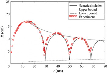
is chosen to fit with the experimental results. In order to validate the asymptotic analysis, a numerical solution is obtained for these parameter values. Figure 1 compares the amplitude envelope of the bubble radius,
 $R_{max}$
and
 $R_{min}$
, with the experimental results and a full numerical solution of (2.4)–(2.7), the agreement being excellent.
Comparison of the time histories of a spherical underwater explosion bubble using a full numerical solution of the Keller–Miksis equation (2.4)–(2.7), the amplitude envelope of the bubble radius and experimental results (Hung & Hwangfu Reference Hung and Hwangfu2010). In this experiment, a special detonator equivalent to 1.32 g of trinitrotoluene is 1.5 m below the water surface. The amplitude envelope employs the solution to (4.2)–(4.3) and the roots of (3.9). The parameter values used in the calculations are the Reynolds number
 $Re\approx 1.9\times 10^{6}$
, the Weber number
 $We\approx 2.7\times 10^{5}$
,
 $p_{g0}\approx 1.22\times 10^{-3}$
(
 $R_{eq}=0.26$
) and the Mach number
 $\unicode[STIX]{x1D716}\approx 0.0073$
.

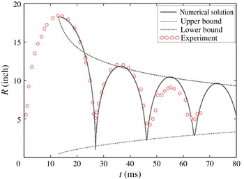
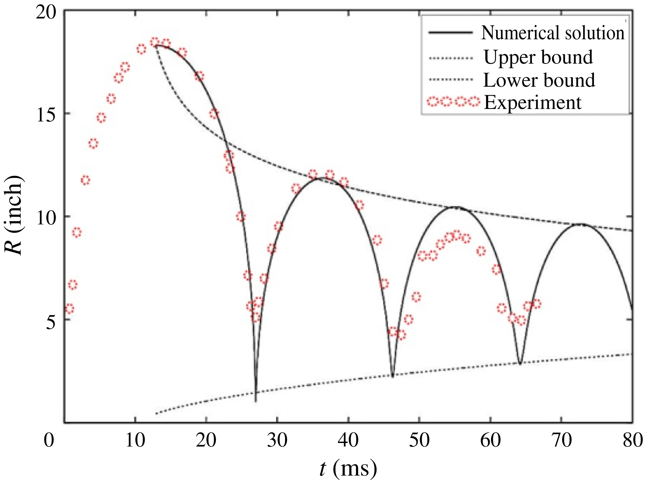
Comparison of the time histories of a spherical underwater explosion bubble using a full numerical solution of the Keller–Miksis equation (2.4)–(2.7), the amplitude envelope of the bubble radius and experimental results (Cole Reference Cole1948). The experiment corresponds to a tetryl charge of 0.249 kg detonated 91.44 m below the water surface. The amplitude envelope employs the solution to (4.2)–(4.3) and the roots of (3.9). The parameter values used in the calculations are the Reynolds number
 $Re\approx 1.5\times 10^{7}$
, the Weber number
 $We\approx 6.4\times 10^{6}$
,
 $p_{g0}\approx 1.63\times 10^{-2}$
(
 $R_{eq}=0.33$
) and the Mach number
 $\unicode[STIX]{x1D716}\approx 0.0214$
.
The logarithm of the rate of change of energy
 $\ln |\text{d}E_{0}/\text{d}t_{c}(0)|$
in (4.2) as a function of (a) the logarithm of the dimensionless initial pressure of the bubble gases
 $\ln (p_{g0})$
for
 $We=10$
and three values of
 $\unicode[STIX]{x1D705}=1.25$
, 1.4, 1.667 and (b) the logarithm of the Weber number
 $\ln (We)$
for
 $p_{g0}=0.01$
and three values of
 $\unicode[STIX]{x1D705}=1.25$
, 1.4, 1.667. The energy corresponds to the initial condition for
 $E_{0}$
in (4.3).

Another case for comparison corresponds to a tetryl charge of 0.249 kg detonated 91.44 m below the water surface (Cole Reference Cole1948). The following values for gas bubbles in water are adopted following the experimental conditions
 $\unicode[STIX]{x1D6E5}=9.9\times 10^{5}~\text{kg}~\text{m}^{-1}~\text{s}^{-2}$
,
 $\unicode[STIX]{x1D70E}=0.0725~\text{Nm}^{-1}$
,
 $\unicode[STIX]{x1D705}=1.25$
,
 $\unicode[STIX]{x1D707}=0.001$
Pa s,
 $c=1500~\text{ms}^{-1}$
,
 $\unicode[STIX]{x1D70C}=998~\text{kg}~\text{m}^{-3}$
and
 $\bar{R}_{max}=0.47$
m. With the above parameters, we deduce that the Reynolds number
 $Re\approx 1.5\times 10^{7}$
, the Weber number
 $We\approx 6.4\times 10^{6}$
and the Mach number
 $\unicode[STIX]{x1D716}\approx 0.0214$
. The dimensionless initial pressure of the bubble gases
 $p_{g0}\approx 1.63\times 10^{-2}$
is chosen to fit with the experimental results. Figure 2 compares the amplitude envelope of the bubble radius,
 $R_{max}$
and
 $R_{min}$
, with the experimental results and a full numerical solution of (2.4)–(2.7). The theoretical results for
 $R_{max}$
and
 $R_{min}$
agree with the Keller–Miksis equation, but there are some discrepancies between the theoretical results and the experimental results. This is because that the bubble becomes non-spherical due to buoyancy after the first cycle of oscillation (Hung & Hwangfu Reference Hung and Hwangfu2010; Wang Reference Wang2013).
The
 $R_{min}$
and
 $R_{max}$
obtained here are the approximated maximum and minimum radii during each cycle of oscillation, which thus only provide an approximate envelope for the oscillating radius history. The errors in our asymptotic approach are of the order of the Mach number
 $\unicode[STIX]{x1D716}$
. It is clear that the errors in our approach, when compared with the numerical solution, are greater in figure 2 for the Mach number
 $\unicode[STIX]{x1D716}\approx 0.0214$
than in Figure 1 for
 $\unicode[STIX]{x1D716}\approx 0.0073$
.
4.2 Energy loss rate:
 $\text{d}E/\text{d}t$

In view of (3.1b
) and (4.2), the loss rate
 $\text{d}E_{0}/\text{d}t$
of the energy of the bubble system is proportional to the Mach number
 $\unicode[STIX]{x1D716}$
. From (4.2)–(4.3), we deduce that
 $\text{d}E_{0}/\text{d}t_{c}(0)=h(p_{g0},\unicode[STIX]{x1D705},We)$
which allows us to analyse how
 $\text{d}E_{0}/\text{d}t_{c}(0)$
varies with
 $p_{g0}$
,
 $\unicode[STIX]{x1D705}$
and
 $We$
.
Figure 3(a) shows
 $\text{d}E_{0}/\text{d}t_{c}(0)$
versus
 $p_{g0}$
in the range
 $[0.01,0.99]$
for
 $We=10$
and
 $\unicode[STIX]{x1D705}=1.25$
, 1.4 and 1.667, respectively. The magnitude of the energy loss rate decreases with the minimum bubble pressure
 $p_{g0}$
, since a bubble at a smaller minimum pressure is associated with a larger pressure difference with the ambient pressure. It thus follows that a stronger collapse is associated with increased energy loss due to acoustic radiation at the end of collapse. The magnitude of the energy loss rate increases inversely with the polytropic index
 $\unicode[STIX]{x1D705}$
, as a smaller
 $\unicode[STIX]{x1D705}$
is associated with stronger collapse. For a smaller
 $\unicode[STIX]{x1D705}$
, the pressure of the bubble gas increases slower during the collapse for the same change in volume, thus leading to a relatively stronger collapse.
Figure 3(b) shows
 $\text{d}E_{0}/\text{d}t_{c}(0)$
versus
 $We$
in the range
 $[10,200]$
for
 $p_{g0}=0.01$
and
 $\unicode[STIX]{x1D705}=1.25$
, 1.4 and 1.667, respectively. The magnitude of the energy loss rate decreases with the
 $We$
number. The surface tension effects are more prominent at a smaller value of
 $\unicode[STIX]{x1D705}$
.
4.3 Influence of the first collapse
Figure 4 shows the influence of the intensity of the first collapse through the parameter
 $p_{g0}$
. In this figure, we have introduced the energy difference between the total energy and the energy of the system in the final equilibrium state
 $E_{eq}$
defined by
 $$\begin{eqnarray}E_{eq}=-\frac{p_{g0}}{3(1-\unicode[STIX]{x1D705})}R_{eq}^{3(1-\unicode[STIX]{x1D705})}+\frac{R_{eq}^{2}}{We}+\frac{1}{3}R_{eq}^{3}.\end{eqnarray}$$
Figure 4(a) shows that the loss rate of the average energy of a bubble system per cycle decreases with the minimum pressure
 $p_{g0}$
at the maximum bubble radius. A smaller
 $p_{g0}$
reflects a larger imbalance of the bubble gas pressure with the ambient pressure and thus is associated with a stronger collapse and greater energy loss. Figure 4(a) also shows that the loss rate of the average energy decreases with the polytropic index
 $\unicode[STIX]{x1D705}$
of the bubble gas, as a smaller
 $\unicode[STIX]{x1D705}$
is associated with a stronger collapse. The minimum bubble radius thus increases with
 $p_{g0}$
and
 $\unicode[STIX]{x1D705}$
, as shown in figure 4(b). Figure 4(c) shows that the frequency of bubble oscillation decreases with
 $p_{g0}$
but increases with
 $\unicode[STIX]{x1D705}$
.
The influence of the first collapse through the parameter
 $p_{g0}$
on (a)
 $E_{0}(0)-E_{eq}$
, (b)
 $R_{min}(E_{0}(0),p_{g0},\unicode[STIX]{x1D705},We)$
, (c)
 $\unicode[STIX]{x1D714}(E_{0}(0),p_{g0},\unicode[STIX]{x1D705},We)$
for three values of
 $\unicode[STIX]{x1D705}=1.25$
, 1.4, 1.667 and
 $We=10$
.

4.4 The behaviour over many cycles
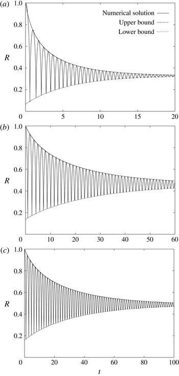
Comparison of the numerical solution to the Keller–Miksis equation (2.4)–(2.7) and the upper and lower bounds evaluated using the solution to (4.2) and the roots of (3.9). The parameter values are
 $We=1.38$
(
 $R_{eq}=0.33$
) for (a),
 $We=13.8$
(
 $R_{eq}=0.45$
) for (b),
 $We=138$
(
 $R_{eq}=0.47$
) for (c),
 $\unicode[STIX]{x1D716}=0.00667$
,
 $p_{g0}=0.05$
and
 $\unicode[STIX]{x1D705}=1.4$
.

Figure 5 compares the numerical solutions of the Keller–Miksis equation (2.4)–(2.7) and the upper and lower bounds evaluated by the present theory. The parameter values used are
 $\unicode[STIX]{x1D716}=0.00667$
,
 $p_{g0}=0.05$
and
 $\unicode[STIX]{x1D705}=1.4$
and
 $We=1.38$
, 13.8, 138, which are corresponding to the dimensional maximum bubble radii
 $\bar{R}_{max}=1,10,100~\unicode[STIX]{x03BC}\text{m}$
, respectively, for a bubble in water with
 $\unicode[STIX]{x1D70E}=0.0725~\text{Nm}^{-1}$
. The bubble undergoes damped oscillation due to acoustic radiation, with the minimum radius increasing, maximum radius decreasing and both of them achieving an equilibrium radius ultimately. They approach the equivalent radius slower for a larger Weber number (or a larger bubble). The upper and lower bounds predicted by the theory agrees excellently with the numerical results for a number cycles of oscillation.
The time histories of (a) the difference between the total energy and the equilibrium energy of the bubble system
 $E_{0}-E_{eq}$
, (b) the maximum bubble radius
 $R_{max}$
, (c) the minimum bubble radius
 $R_{min}$
and (d) the oscillation frequency
 $\unicode[STIX]{x1D714}$
of the bubble. The initial condition for (4.2) is taken from the second maximum value of the radius in the numerical solution. The parameter values are
 $We=1.38$
, 13.8, 138,
 $\unicode[STIX]{x1D716}=0.00667$
,
 $p_{g0}=0.001$
and
 $\unicode[STIX]{x1D705}=1.4$
.

Figure 6 displays the time histories of the difference between the total energy and the equilibrium energy of the bubble system, maximum and minimum radii and oscillation frequency of the bubble. The energy difference of the bubble system
 $E_{0}-E_{eq}$
initially decreases rapidly and the rate of change decreases rapidly too (figure 6
a). For a larger
 $We$
number (or a larger bubble), the energy decreases slower. For a larger
 $We$
number (or a larger bubble), the maximum radius decreases slower, reaching an equilibrium status later but at a larger equilibrium radius (figure 6
b,c). The oscillation frequency increases with time, increasing faster and reaching at a larger equilibrium value at a short period for a smaller
 $We$
number (or a smaller bubble) (figure 6
d).
5 Summary and conclusions
A theoretical study has been carried out to investigate the acoustic decay of nonlinear oscillations of a spherical bubble in a compressible inviscid fluid, using the Keller–Miksis equation. This is a multi-scaled problem with a short time scale associated with inertial oscillation and a long time scale associated with acoustic damping, their ratio being the Mach number. A multi-scaled perturbation method is thus employed to solve the Keller–Miksis equation. The techniques of strongly nonlinear analysis result in several important analytical formulae including the following.
(i) The leading-order analytical solution of the bubble radius history is obtained to the Keller–Miksis equation in a closed form including both compressible and surface tension effects.
(ii) An explicit expression for the average energy loss rate for the bubble system for each cycle of oscillation, which allows the calculation of the energy loss without prior knowledge of the bubble radius history.
(iii) An explicit formula is obtained for the dependence of the frequency of oscillation on the energy.
(iv) Implicit formulae are obtained for the maximum and minimum radii of the bubble during each cycle of oscillation.
These asymptotic predictions have excellent agreement with experimental results and the numerical solutions of the Keller–Miksis equation over the long lifetime of the damped oscillations of a transient bubble in a compressible liquid. Theoretical and numerical studies are undertaken with the above formulae for the energy of the bubble system, frequency of oscillation and minimum/maximum bubble radii in terms of the dimensionless initial pressure of the bubble gases
 $p_{g0}$
, the Weber number
 $We$
and polytropic index of the bubble gas
 $\unicode[STIX]{x1D705}$
. The following new phenomena/features are observed:
The energy loss rate of a bubble system is proportional to the Mach number
 $\unicode[STIX]{x1D716}$
. This is as expected since the energy loss is associated with acoustic radiation, which increases with the Mach number.
The energy loss rate decreases with the minimum bubble pressure
 $p_{g0}$
and the polytropic index
 $\unicode[STIX]{x1D705}$
of the bubble gas. A smaller
 $p_{g0}$
reflects the stronger imbalance between the bubble internal pressure and ambient pressure, and thus is associated with stronger collapse. A smaller
 $\unicode[STIX]{x1D705}$
is associated with weaker collapse.
For a smaller
 $We$
(or stronger surface tension), the equilibrium bubble radius and equilibrium energy increase, since surface tension acts as an elastic parameter of the oscillation bubble system.