1 Introduction
The Schrödinger equation in quantum mechanics is a partial differential equation describing the evolution of the quantum state of the physical system with time, and is one of the fundamental equations of quantum mechanics. It reveals the basic law of the matter movement in the microscopic physical world. It is a powerful tool for dealing with all non-relativistic problems in atomic physics, and is widely applied in atomic, molecular, solid-state physics, nuclear physics, chemistry and other fields.
The nonlinear Schrödinger equation (NLSE) is related to various nonlinear problems in theoretical physics, such as nonlinear optics, fluid mechanics, condensed matter physics, electromagnetism and ionic acoustic waves of plasmas (Zakharov Reference Zakharov1972; Pereira & Stenflo Reference Pereira and Stenflo1977; Goldman Reference Goldman1984; Silberberg Reference Silberberg1990; Sulem & Sulem Reference Sulem and Sulem1999; Porras Reference Porras2010). The NLSE has been widely applied to describe different kinds of nonlinear waves in physics, such as the propagation of a laser beam in a medium whose refractive index is related to the wave amplitude, the propagation of an optical pulse in a nonlinear dispersive medium, the water wave of an ideal fluid on a free surface and plasma waves. Since the nonlinear Schrödinger equation is a nonlinear partial differential equation, only numerical solutions can be obtained except for some special one-dimensional NLSEs (Pereira & Stenflo Reference Pereira and Stenflo1977; Nie & Li Reference Nie and Li2020). The numerical methods for solving the NLSE include two categories, the finite difference method and the pseudo-frequency spectrum method. In contrast to the finite difference method, the pseudo-frequency spectrum method is one to two orders of magnitude faster under the same accuracy condition, and the step-by-step Fourier transform method is a kind of pseudo-frequency spectrum method widely used to solve the pulse transmission problem of nonlinear dispersion media, and it is a fast and efficient numerical method (Bernatz Reference Bernatz2010).
In recent years, the standard NLSE has been applied to the formation, properties, other local structures and interactions of solitons. Pereira and Stenflo considered the one-dimensional complex coefficient cubic NLSE and obtained the soliton solution by using the approximate estimation method (Pereira & Stenflo Reference Pereira and Stenflo1977). Subsequently, this equation was widely extended to the study of singular solitons, vortices, specklegram and other results (Gupta, Som & Dasgupta Reference Gupta, Som and Dasgupta1981; Conway & Riecke Reference Conway and Riecke2007; Shukla et al. Reference Shukla, Bingham, Phelps and Stenflo2009; Bernatz Reference Bernatz2010; Skarka, Aleksic & Leblond Reference Skarka, Aleksic and Leblond2010). In recent decades, the phenomenon of wave collapse (amounting to the mathematical singularity problem) often appears in many theoretical studies of nonlinear wave interaction. The study of wave collapse is also based on the NLSE (Grindrod Reference Grindrod1966; Zakharov Reference Zakharov1972; Grimes & Adams Reference Grimes and Adams1979; Goldman Reference Goldman1984; Zakharov, Musher & Rubenchik Reference Zakharov, Musher and Rubenchik1985; Musher, Rubenchik & Zakharov Reference Musher, Rubenchik and Zakharov1995; Sulem & Sulem Reference Sulem and Sulem1999; Kivshar & Pelinovsky Reference Kivshar and Pelinovsky2000). When both the group dispersion coefficient $p=p_r+{\rm i}p_i$ and the nonlinear coefficient $q=q_r+{\rm i}q_i$
 in the nonlinear Schrödinger equation are complex constants, it is also called the generalized nonlinear Schrödinger equation(GNSE). It is also a kind of generalized nonlinear reaction–diffusion equation. Different kinds of novel instability phenomena have been found successively through a numerical study based on the two-dimensional GNSE. Zhao & Yu (Reference Zhao and Yu2011), Zhao et al. (Reference Zhao, Tian, Cui and Yu2012), Cui, Yu & Zhao (Reference Cui, Yu and Zhao2013), Yu, Cui & Zhao (Reference Yu, Cui and Zhao2015) and Cui, Lv & Xin (Reference Cui, Lv and Xin2016) found that the localized large-amplitude pulse first undergoes modulational instability and then collapses into the shortest-wavelength modes, and then the collapse is followed by the inverse cascade of energy back to modes of longer wavelengths, until a stationary state homogeneous turbulence with a spiky energy spectrum appears. Further, Cui et al. (Reference Cui, Yu and Zhao2013), Yu et al. (Reference Yu, Cui and Zhao2015) and Cui et al. (Reference Cui, Lv and Xin2016) found that the inverse cascade or decay following the collapse can then lead to asymptotic states with nearly single-mode-dominated turbulence and, finally, the energy was condensed in the same wavenumber $|k|$
 mode with eight phase angles in the phase space, or near the terminals of three different wave vectors, rather than into the homogeneous turbulence state filling the whole space.
In this paper, we mainly focus on the analysis of the wave inverse cascade instability with a simple self-regulating feedback control based on a two-dimensional GNSE. As expected (Zhao & Yu Reference Zhao and Yu2011; Zhao et al. Reference Zhao, Tian, Cui and Yu2012; Cui et al. Reference Cui, Yu and Zhao2013; Yu et al. Reference Yu, Cui and Zhao2015; Cui et al. Reference Cui, Lv and Xin2016), at the start of the evolution the initial pulse firstly suffers the modulation instability, followed by collapse into the shortest-wavelength modes in the system. This is followed by the inverse cascade of the shortest-wavelength modes back to the longer-wavelength ones, until a statistical stationary turbulent state is reached. And the inverse cascade is limited to the shorter-wavelength modes with the wavenumber $|k|\geq 100$ . The viscous damping $p_i$
 plays an important part in the process of the inverse cascade. Under the self-regulating feedback control in the system, the inverse cascade can be regulated in a way.
2 Generalized NLSE
The two-dimensional GNSE including a simple self-regulating feedback control term can be written as follows:

where it is applied to describe the evolution of instability with time in the electron plasma wave packet field. In (2.1), $E(x,y,t)$ is a complex wave packet function of space position $(x,y)$
 and time $t$
 , $V(x,y)$
 represents the initially given external potential energy, ${\rm i}$
 is the imaginary unit and $i^2=-1$
 . ${\nabla }^2$
 is a Laplace operator which satisfies

Equation (2.1) is different from the standard cubic NLSE, here, both the group dispersion coefficient $p=p_r+{\rm i}p_i$ and the nonlinear coefficient $q=q_r+{\rm i}q_i$
 are complex constants, where $p_r$
 is the coefficient of group velocity dispersion $p_r{\nabla }^2E$
 , and $p_i$
 is the coefficient of viscous damping (growth) determined by wavelength $p_i{\nabla }^2E$
 . Also, $q_i$
 is the coefficient of growth (damping) determined by amplitude, $q_r|E|^2E$
 is the nonlinear frequency shift of dispersion and $q_i|E|^2E$
 is the nonlinear damping (growth). The last term $\beta |E{|^2}(\beta \ne 0)$
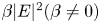 is a feedback control term in the system; when $\beta = 0$
 there has no feedback control in the system.
In this paper, we study the evolution of the initial perturbation of the local finite amplitude with time under a given external potential energy. In general, the total energy is not conserved (except $p_i=q_i=0$ ). The evolution of the total wave energy $w=\iint _{D}|E(t,x,y)|^2\,{\rm d}x\,{\rm d}y$
 (where $D$
 is the whole $xy$
 plane region) can be obtained from (2.1)

This shows that positive values of $p_i$ and $q_i$
 , respectively, correspond to gain and loss of the total wave energy. For non-dissipative systems, $w$
 is conserved.
The external potential energy is given by

Here, $V_0=-3.0,a=5.0,b=6.0$ . As for the form of the external potential energy equation, many kinds of forms have been tried by trial and error, and it has finally been found that the different forms have less influence on the analysis. The initial pulse is given by

Here, $E_0=0.05,r_0=2.0$ . The spatial structures of the external potential and the initial perturbation are shown in figure 1.
External potential and initial perturbation.

The simulation region is $D=[-2{\rm \pi},2{\rm \pi} ;-2{\rm \pi},2{\rm \pi} ]$ under the periodic boundary conditions. It can be seen from figure 1 that a small perturbation is given at the initial time in the system. It is in the centre of the simulation region and has a narrow spatial contour, and the amplitude is obviously smaller than the external potential energy $|V(x,y)|$
 . The evolution process of the initial small disturbance with time is studied based on the GNSE. In this paper, the GNSE is numerically solved using the spectral method by carrying out the step-by-step Fourier transform method in space and a fourth-order Runge–Kutta method in time. The number of grids is $256\times 256$
 , and the time step is ${\Delta t}=10^{-3}$
 . We also have verified that the grids are sufficiently fine to ensure low level aliasing effects and the absence of preferential alignment of small turbulence structures.
3 Numerical results
3.1 In the absence of feedback control in the system
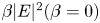
The GNSE is investigated numerically for $p=3.5+0.5{\rm i},q=8.0+0.9{\rm i}$ in the absence of the feedback control term $\beta |E{|^2}(\beta =0)$
 . We consider a system with positive group dispersion $p_r>0$
 , viscous heating $p_i>0$
 , nonlinear frequency upshift $q_r|E|^2>0$
 and nonlinear damping $q_i|E|^2>0$
 , as well as an external potential $V(x,y)$
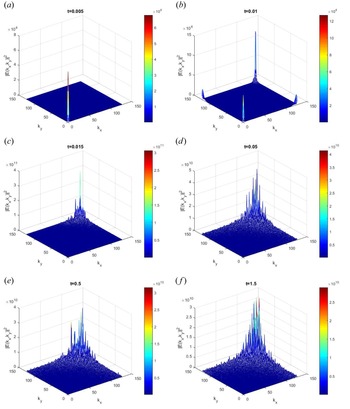
 . Figure 2 shows a quadrant of the evolution of energy spectrum $|E(t,k_x,k_y)|^2$
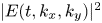 at $t=0.005,0.01,0.015,0.05,0.5,1.5$
 .
Evolution of energy spectrum $|E(k_x,k_y)|^2$ with time for $p=3.5+0.5{\rm i}, q=8.0+0.9{\rm i}$
 .

It is clearly found in figure 2 that the localized large-amplitude pulse first condenses, forming an intense spot in the small $k$ (long-wavelength) corner, that is, the pulse undergoes modulational instability at time $t=0.005$
 . In a very short time, a part of the instability energy has been transferred to the shortest-wavelength region (large wavenumber $k$
 ) allowed by the system at time $t=0.01$
 . After a while, at around $t=0.015$
 , the energy has been completely transferred to the shortest-wave region (maximum wavenumber $k$
 ), and the initial pulse has evolved into the shortest-wave modes. The whole process is a very typical wave collapse process (Grindrod Reference Grindrod1966; Zakharov Reference Zakharov1972; Grimes & Adams Reference Grimes and Adams1979). In this case, the wave collapse occurs quickly, and the energy of the system quickly increases. Soon the short-wave modes gradually develop to the longer-wave modes (the value of $k$
 is smaller), and there is onset of the inverse cascade instability. Unlike before (Cui et al. Reference Cui, Yu and Zhao2013; Yu et al. Reference Yu, Cui and Zhao2015; Cui et al. Reference Cui, Lv and Xin2016), the inverse cascade energy remains in the shorter-wave region (the smaller wavenumber $k$
 ) for a long time until $t=1.5$
 . We also can see that the system energy is concentrated in the $k$
 ($|k|\geq 100$
 ) space region, and the short-wave mode energy is higher than the longer-wave mode energy. Generally, the relative stable region forms a round domain with radius $|k|=100$
 in the whole $k$
 space.
Figure 3 shows the evolution of the total energy of the system $\iint _{D}|E(t,x,y)|^2\,{\rm d}x\,{\rm d}y$ with time for $p=3.5+0.5{\rm i},q=8.0+0.9{\rm i}$
 . It can be seen from figure 3 that, at initial time $(t<0.01)$
 , the total energy of the system is close to zero. At the time $t=0.01$
 , the total energy rises in a straight line and rapidly. increases to the highest point (singularity). Meanwhile, the wave collapse phenomenon occurs in the whole system, and then, in a very short time, the system energy decreases sharply until $t=0.02$
 , and then the energy of the whole system fluctuates around a stable value.
Evolution of total system energy $\iint _{D}|E(t,x,y)|^2\,{\rm d}x\,{\rm d}y$ for $p=3.5+0.5{\rm i},q=8.0+0.9{\rm i}$
 .

The viscous damping (growth) $p_i$ in the GNSE is determined by the wavelength. The effect of $p_i$
 on the inverse cascade instability is investigated. By fixing the parameters in the GNSE except $p_i$
 , and gradually increasing the value of $p_i(\geq 0.5)$
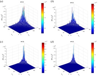
 , figure 4 shows the comparison of the system energy spectrum $|E(k_x,k_y)|^2$
 at time $t=1.5$
 for $p_i=0.5,0.6,0.8,1.0$
 . It can be clearly seen from figure 4 that the short-wave mode region of the inverse cascade is gradually reduced with the increase of the value of $p_i$
 , that is, the increase of the value $p_i$
 in this case can suppress the inverse cascade process. Meanwhile, it is found that the solution of (2.1) diverges to infinity for $p_i\geq 1.1$
 .
Comparison of system energy spectrum $|E(1.5,k_x,k_y)|^2$ ; (a) $p_i=0.5$
 , (b) $p_i=0.6$
 , (c) $p_i=0.8$
 , (d) $p_i=1.0$
 .

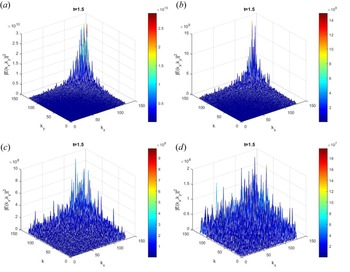
Figure 5 shows the comparison of the system energy spectrum $|E(k_x,k_y)|^2$ at the time $t=1.5$
 for $p_i=0.5,0.4,0.2,0.1$
 . It is found that the inverse cascade process gradually expands to the long-wave region when the value of $p_i$
 decreases. While $p_i=0.1$
 , the system energy transfers back to the long-wave region, and eventually the whole $k$
 phase space is filled with a spiky turbulent state.
Comparison of system energy spectrum $|E(1.5,k_x,k_y)|^2$ ; (a) $p_i=0.5$
 , (b) $p_i=0.4$
 , (c) $p_i=0.2$
 , (d) $p_i=0.1$
 .

By analysing figures 4 and 5, it is easily found that the inverse cascade process can be regulated by the viscous damping $p_i$ for $p_r=3.5,q=8.0+0.9{\rm i}$
 . The larger the value of $p_i$
 is, the smaller the inverse cascade process is. When the value of $p_i$
 varies from $0.1$
 to $1.0$
 , the viscous coefficient $p_i$
 determined by the wavelength acts as a regulating switch, which can regulate the inverse cascade process in a way.
3.2 With feedback control in the system
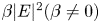
The GNSE is investigated numerically for $p=3.5+0.5{\rm i},q=8.0+0.9{\rm i}$ with a simple feedback control term $\beta |E{|^2}(\beta \ne 0)$
 . Figure 6 shows the evolution of total energy $\iint _{D}|E(t,x,y)|^2\,{\rm d}x\,{\rm d}y$
 for the different levels of self-regulated feedback control $\beta |E{|^2}$
 . One can see the total energy of the system is close to zero at the initial time $(t<0.01)$
 . At approximately $t=0.01$
 , the total energy for the different $\beta$
 transforms in a vertical straight line and rapidly increases to the highest point (singularity) almost at the same time. The mode amplitudes are unequal for the different feedback control values $\beta |E{|^2}$
 in the singular point, and the amplitude is the least when $\beta =0$
 . Meanwhile, the wave collapse occurs in the four systems, and the feedback control affects the wave collapse amplitude, whereafter the system energy sharply decays until approximately $t=0.015$
 . From $t=0.015$
 to $t=0.02$
 , there are obviously larger fluctuations in the system for $\beta \ne 0$
 . From $t=0.02$
 , the four kinds of system energy all fluctuate around a stable value. In this case, the right-hand side of (2.3) can vanish during the evolution, so that the total energy becomes constant, i.e. the summed effect of growth and damping of all the modes in the system become balanced.
Evolution of total system energy $\iint _{D}|E(t,x,y)|^2\,{\rm d}x\,{\rm d}y$ for $\beta =0,5,10,20$
 ; (a) $\beta =0$
 , (b) $\beta =5$
 , (c) $\beta =10$
 , (d) $\beta =20$
 .

Fixing $p=3.5+0.5{\rm i},q=8.0+0.9{\rm i}$ under a simple feedback control $\beta |E{|^2}(\beta \ne 0)$
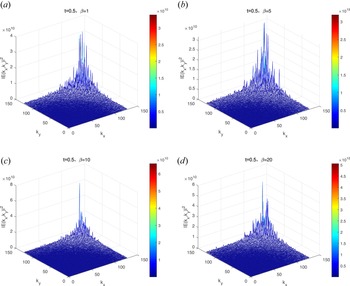
 in (2.1), we present the energy spectrum $|E(k_x,k_y)|^2$
 at $t=0.5$
 with various $\beta$
 values (different levels of self-regulated feedback control $\beta |E{|^2}$
 ) in figure 7. One can see that, for small $\beta =1$
 , the inverse cascade energy spectrum is similar to that for $\beta =0$
 . For $\beta =5$
 and 10, the shorter-wave mode slowly converts to a longer-wave mode. However, even for large $\beta =20$
 , there is also mode conversion. This can explain how the feedback controls invoked here regulate the mode amplitudes, and the inverse cascade mode process is mainly determined by the viscous damping.
Value of $|E(k_x,k_y)|^2$ for different levels of self-regulated feedback control at $t=0.5$
 ; (a) $\beta =1$
 , (b) $\beta =5$
 , (c) $\beta =10$
 , (d) $\beta =20$
 .

4 Conclusion
This research has analysed the entire evolution of a pulse disturbance in a plasma modelled by the two-dimensional GNSE including group dispersion, diffusion, dissipation and self-regulated feedback control. The total system energy can become balanced during the evolution. The system here is open and non-conservative, and existing theories such as resonant three-wave interaction and wave kinetic equations do not work (Sagdeev & Galeev Reference Sagdeev and Galeev1969; Stenflo Reference Stenflo1994; Mendonça & Bingham Reference Mendonça and Bingham2002; Mendonça & Hizanidis Reference Mendonça and Hizanidis2011). For the two-dimensional GNSE, it is unable to obtain a definite theoretical description, so we can get some results from numerical simulation. In the absence of self-regulated feedback control, $\beta |E{|^2}(\beta =0)$ , as expected, modulation instability, wave collapse and inverse cascade occur one after another until a statistical stationary turbulent state is reached. Different from the previous results, it is found that the perturbation energy after the inverse cascade is mainly concentrated in the region $|k|\geq 100$
 under $p=3.5+0.5{\rm i},q=8.0+0.9{\rm i}$
 , i.e. the inverse cascade is limited to the shorter-wavelength mode region. Meanwhile, a regular relative circular stable region appears for $|k|\leq 100$
 (long-wavelength modes region).
The viscous damping $p_i$ is an important factor in the evolution. It is found that the energy in the short-wave region shrinks gradually with increasing $p_i(0.5< p_i\le 1.0)$
 . The regular relatively stable region expands continuously. While reducing the imaginary part $p_i(0.1\le p_i<0.5)$
 gradually, the regular relatively stable region is continuously reduced until it disappears, and the inverse cascade fills the whole space in a sharp-fork turbulent state. The viscous damping $p_i$
 acts like a control switch for the process of inverse cascade. Under a simple self-regulated feedback control $\beta |E{|^2}(\beta \ne 0)$
 , it is clearly found that the feedback control acts like a switching mechanism. Our results can be directly applied to laser filamentation (Liao, Kelley & Ouellette Reference Liao, Kelley and Ouellette2012), Langmuir wave turbulence (Robinson Reference Robinson1997) and other phenomena governed by two-dimensional GNSE in material science, fluid dynamics, atomic and plasma physics, biology and other areas (Grindrod Reference Grindrod1966; Grimes & Adams Reference Grimes and Adams1979; Murray, Sprenger & Wenk Reference Murray, Sprenger and Wenk1990; Murray Reference Murray1993; Aranson & Kramer Reference Aranson and Kramer2002; Reis, Ingale & Shattuck Reference Reis, Ingale and Shattuck2006). The new nonlinear state and the more useful feedback control in the improved nonlinear system remain to be discovered.
Acknowledgements
The authors thank Professor M.Y. Yu for valuable discussions and the anonymous referees for valuable feedback.
Editor Steve Tobias thanks the referees for their advice in evaluating this article.
Funding
This work was supported by the National Natural Science Foundation of China (grant number 11105065), the Outstanding Youth Innovation Team Project of Shandong Higher Education Institution (grant number 2021KJ042).
Declaration of interests
The authors report no conflict of interest.