NOMENCLATURE
- ATM
air traffic management
- BADA 4.0
base of aircraft data version 4.0 – an aircraft performance model
- CAS
calibrated air speed [Kn]
- DM
decision maker
- EA
evolutionary algorithms
- EST
Eastern Standard Time
- EOC
end of cruise
- FAA
Federal Aviation Administration
- FPL
flight plan
- fpm
feet per minute (1fpm = 1ft/min)
- GA
genetic algorithms
- GDPS
Global Deterministic Prediction System
- GRIB2
GRIdded Binary 2 data file format
- IDLE
Idle thrust engine setting
- JFK
John F. Kennedy Airport
- Kn
knots [NM/h]
- LFPL
lateral flight plan
- LHR
London Heathrow Airport
- MACH
Mach speed [-]
- MCMB
maximum climb thrust engine setting
- MCRZ
maximum cruise thrust engine setting
- MMO
maximum operational MACH speed limit [-]
- MOO
multi-objective optimisation
- NAT-OTS
North Atlantic Organized Track System
- NG-FMS
New Generation Flight Management System
- NSGA-II
non-dominated sorting genetic algorithm II
- NM
nautical miles
- M i
number of non-empty tentative solutions at iteration i
- m i
number of updated tentative solution elements at iteration i
- ORT
orthodromic route
- P-ORT
orthodrome constructed perpendicular to the ORT
- P 0
initial population
- P i
population of generation i
- RGRID
routing grid
- RTA
Required Time of Arrival [h]
- RTA n
nth RTA constraint value
- SLL
Sea level length – the length of a flight segment computed at the SLA
- TAP
traffic aware planner
- TBO
trajectory-based operations
- TOC
top of climb
- TOD
top of descent
- TS
tentative solutions set
- TS i
tentative solution set at iteration i
- UTC
Coordinated Universal Time
- VFPL
vertical flight plan
- VMO
Maximum Operational CAS speed limit [Kn]
- WGS84
World Geodetic System 1984 – ellipsoid earth model
- TLA
thrust lever angle (engine thrust setting) [%]
- WPT
waypoint
- WPT final
final flight trajectory point/lateral flight plan
- WPT init
Initial flight trajectory point/lateral flight plan
- ΔRTA
RTA constraint window width
- 4D
four-dimensional space (latitude, longitude, altitude and time)
1.0 INTRODUCTION
This paper presents a new optimisation method designed to support Decision Makers (DMs) in the planning phase of flights with a Required Time of Arrival (RTA) constraint at the final waypoint (WPT final). The proposed flight trajectory optimisation method may be applied in future operational paradigms, such as Trajectory-Based Operations (TBO)/free flight, where aircraft do not need to follow predetermined routes.
Aircraft flight trajectories are the result of two levels of planning, optimisation and validation: local (aircraft), and global (airspace). At the aircraft level, the flight trajectory planning, optimisation, and validation are performed by aircraft operators/the Flight Management System (FMS)/an aircrew(Reference Ng, Sridhar and Grabbe1-Reference Patrick and Sheridan3), based on specific flight data (aircraft performance data and limitations, load, departure/destination pair, atmospheric conditions, navigation constraints, etc.). The result is a flight profile that minimises a preselected cost function (fuel burn, total costs, flight time, etc.), and satisfies all constraints and regulations(4). At the global level, the Air Traffic Management (ATM) system(Reference Fanti, Pedroncelli, Stecco and Ukovich5-Reference Cate9) performs the optimisation and validation. The objective is to ensure safe operations for all aircraft in that airspace (aircraft separation, compliance with navigation rules, regulations and policies, etc.) and to maximise the airspace throughput. The optimal flight trajectory selected by the flight operator is defined as a Flight Plan (FPL)(10,Reference Altus11) . A FPL is a standard, structured format, flight trajectory description, and is submitted to ATM for validation and approval. If the FPL is rejected, the flight planning sequence is repeated. In the near future, upon the implementation of time-based metering operation in the US airspace(Reference Underwood, Cotton, Hubbs, Vincent, Sagar and Karr12), at certain points in the airspace (geographic locations and altitudes) where the traffic demand is high, a time constraint (RTA constraint), negotiated between the flight planner and the ATM, will be assigned to each aircraft, which will have to cross the location within its assigned time window.
An aircraft can fly at any altitude–speed combination within its flight envelope. Although this is the case, the FPL segments have discrete speed and altitude values. The discrete speed values (multiples of 1Kn for Calibrated Air Speed (CAS), and 0.001 for MACH) are a result of the limitations regarding their selectable values in the FMS and the Flight Control Unit (FCU). Cruise altitudes are multiple of 1,000ft, as imposed by navigation regulations.
Some examples of flight trajectory optimisation problems treated in the literature as a flight-planning problem are presented in refs. [Reference Di Vito, Corraro, Ciniglio and Verde13-Reference Woods, Vivona, Roscoe, LeFebvre, Wing and Ballin20]. The Aircraft’s Performance Model (APM), the Atmospheric Data Model (ADM), the specific optimisation problem (initial aircraft position and speed, weight, fuel quantity, etc.) and the method/approach, etc., influence the results of the optimisation: the flight trajectories/flight plans identified as solutions and their qualities.
The type of APM used in flight performance calculations differs as a function of the context and platform on which they are conducted. In ATM platforms, the flight performance calculations are performed on ground-based computers, using an aero-propulsive aircraft model (e.g. BADA(Reference Nuic, Poles and Mouillet21-24)) that is more complex and more accurate than other models. In current FMS platforms, on-board systems with limited computational power, the flight performance calculations are performed using an APM based on interpolation tables (Performance Database – PDB)(Reference Murrieta-Mendoza and Botez25,Reference Sibin, Guixian and Junwei26) , which are less accurate and less complex. Ramasamy et al.(Reference Ramasamy, Sabatini, Gardi and Liu27,Reference Ramasamy, Sabatini, Gardi and Kistan28) presented concepts for a New Generation Flight Management System (NG-FMS) architecture and flight trajectory optimisation algorithms. The APM can be provided either by the aircraft manufacturer or could be generated/estimated based on flight test data. Ghazi and Botez presented a method to generate an APM(Reference Ghazi and Botez29) and an engine model(Reference Ghazi, Botez and Achigui30), based on test flight data. Murietta et al.(Reference Murrieta-Mendoza, Demange, George and Botez31) devised a method for generating a cruise phase PDB from flight test data generated with a level D flight simulator. Ghazi et al.(Reference Ghazi, Botez and Tudor32) presented a method to generate a climb phase PDB from an aero-propulsive aircraft model created from flight test data obtained using and level D flight simulator for Cessna Citation X. Dancila et al.(Reference Dancila, Botez and Labour33) developed a new method that estimates, faster and more precisely, the fuel burn for a cruise segment at constant altitude and the time required to burn a specified quantity of fuel.
The atmospheric data (air temperature and wind predictions) are issued by national meteorological service agencies in a gridded format (GRIB2(34,35) ), and in various forecast models. Atmospheric data are defined in the nodes of a four-dimensional (4D) grid (latitude, longitude, pressure altitude, and time). The differences between the forecast models refer to the area covered by the forecast (global(36,Reference Buehner, McTaggart-Cowan, Beaulne, Charette, Garand, Heilliette, Lapalme, Laroche, Macpherson, Morneau and Zadra37) or regional(38,Reference Caron, Milewski, Buehner, Fillion, Reszka, Macpherson and St-James39) ), the grid resolution, map projection type (latitude–longitude or polar-stereographic), forecast timespan and update interval. Various studies evaluated the forecast data accuracy relative to the real atmospheric conditions encountered by aircraft(Reference Cole, Green, Jardin, Schwartz and Benjamin40-Reference Bronsvoort, McDonald, Potts and Gutt42), and interpolation methods(Reference Stohl, Wotawa, Seibert and Kromp-Kolb43,Reference Stohl44) . The atmospheric conditions (wind and air temperature) along the flight trajectory have an important effect on the aircraft’s flight performance (flight envelope limitations, fuel burn rate, etc.) and its global performance (fuel burn and flight time). Therefore, the atmospheric data used in calculations should be as close as possible to the real atmospheric conditions encountered by the aircraft. A review of the available atmospheric data, their sources and their integration in a prototype route optimisation tool developed by NASA, called the Traffic Aware Planner (TAP) application, is presented in ref. [Reference Lewis, Burke, Underwood and Wing45].
Similar to the APM, ADMs vary as a function of the optimisation context/platform, timespan and area delimiting the flight trajectory. In FMS platforms, given their limited computational power and memory, the atmospheric data are considered stationary, defined in a selected set of points along the flight trajectory, at a limited set of altitudes(Reference Bronsvoort, McDonald, Potts and Gutt42). The atmospheric conditions in a point of interest, other than where the data were defined, are computed by multi-linear interpolations(Reference Stell46-Reference De Smedt and Berz48). In online ATM platforms, the atmospheric data are computed from forecast data(Reference Wickramasinghe, Harada and Miyazawa16,Reference Wynnyk41) by linear interpolations, as a trade-off between precision and computation time. Dancila and Botez(Reference Dancila and Botez49) developed a new ADM that defines the time-varying atmospheric data in the nodes of a Routing Grid (RGRID). The model computes the atmospheric parameter values in a grid node on average six times faster and with the same accuracy as when calculated by 4D interpolations from GRIB2 data.
In flight performance prediction and flight planning/optimisation applications, an aircraft flight trajectory is determined by performing an accelerated simulation of the FPL. The methodology for performing the accelerated simulation and the performance data calculation is described in refs. [Reference Schreur50,Reference Karr, Vivona, Woods and Wing51]. The optimal solution to a flight planning/trajectory optimisation problem is the result of a search. The search identifies, as a function of the optimisation objective, the lateral flight trajectory (Lateral Flight Plan – LFPL), the vertical flight trajectory (Vertical Flight Plan – VFPL – the speed and altitude profile), or both, that minimise a selected cost function and satisfy the imposed constraints. The search is performed within a candidate solution set, selected as a function of the optimisation scenario. Dancila and Botez(Reference Dancila and Botez52) proposed a method to construct a family of vertical flight profiles that cover the aircraft’s flight envelope, appropriate for use in FMS flight trajectory computation and optimisation. Geometrical approaches to vertical flight trajectory optimisation are presented in refs. [Reference Dancila, Beulze and Botez53,Reference Dancila, Beulze and Botez54]. Yu and Zhang(Reference Yu and Zhang55) presented a survey of Unmanned Aerial System (UAS) flight path planning approaches. Ceruti and Marzocca(Reference Ceruti and Marzocca56) modelled the docking manoeuvre of an airship by Bezier curves and proposed an optimisation method using Particle Swarm Optimisation (PSO) to determine the optimal Bezier curve parameters that minimise the energy necessary for the manoeuvre.
For constrained optimisation problems, some constraints apply to the candidate profile set (e.g. altitudes, speeds, waypoints (WPTs), etc.) and others refer to solution attributes (e.g. time constraint(s), etc.). Liden(Reference Liden57) showed that when a flight trajectory is defined by an LFPL and a VFPL that contains a set of segments flown at a set of constant speeds and altitudes, the flight time as a function of speed might contain discontinuities (there are no FPL segment speed and altitude combinations that yield a flight time within a time domain).
Hagelauer and Mora-Camino(Reference Hagelauer and Mora-Camino58) proposed a Dynamic Programming (DP) optimisation method for 4D trajectories with multiple RTA constraints along the route, defined as a control problem, where the search space was reduced using a heuristic. Other authors used an approach based on Evolutionary Algorithms (EAs) for solving the optimisation problem of a flight trajectory with an RTA constraint. Murietta-Mendoza et al.(Reference Murrieta Mendoza, Bunel and Botez59) used an artificial bee colony optimisation algorithm to determine the optimum vertical flight profile for a cruise segment with RTA constraint. The vertical flight profile was then processed to obtain a vertical flight profile with a minimum number of speed changes. Gardi et al.(Reference Gardi, Sabatini and Ramasamy60) presented a review of the multi-objective 4D flight trajectory optimisation methods, in which the cost functions incorporate operational costs, as well as other cost elements such as noise, polluting emissions, contrails, airspace congestion, etc. Flight guidance and control concepts(Reference Ballin, Williams, Allen and Palmer2,Reference Diaz-Mercado, Lee, Egerstedt and Young61) were developed to generate optimal 4D trajectories with a set of RTA constraints assigned at WPTs along the flight trajectory.
Ceruti et al.(Reference Ceruti, Voloshin and Marzocca62) presented a multidisciplinary optimisation approach that uses heuristic optimisation strategies, appropriate for the case where the optimisation involves multiple interdependent parameters. Another multidisciplinary optimisation method presented by Ceruti et al.(Reference Ceruti, Fiorini, Boggi and Mischi63) assigns a fitness value for a candidate solution based on two extreme solutions (an ideal best and an ideal worst solutions) determined for each iteration of the algorithm.
Multi-Objective Optimisation (MOO) algorithms are used extensively to solve problems where the solution must satisfy multiple competing and contradictory objectives. Marler and Arora(Reference Marler and Arora64) conducted a survey of the MOO methods used in engineering. Miettinen(Reference Miettinen, Zitzler, Thiele, Deb, Coello Coello and Corne65) presented the concepts related to MOO and described a series of approaches and methods to conduct the optimisation. Fonseca and Fleming(Reference Fonseca and Fleming66) presented an analysis of MOO methods based on Genetic Algorithms (GAs). Murata and Ishibuchi presented examples of MOO methods based on GAs: an outline for conducting MOO using GAs (MOGA(Reference Murata and Ishibuchi67)), and local search methods(Reference Ishibuchi and Murata68,Reference Ishibuchi and Murata69) . Fonseca and Fleming proposed a MOO method for optimisation problems with multiple constraints, based on EAs(Reference Fonseca and Fleming70,Reference Fonseca and Fleming71) . Deb et al.(Reference Deb, Pratap, Agarwal and Meyarivan72) presented an elitist MOO algorithm based on GAs and non-dominated population sorting (Non-dominated Sorting Genetic Algorithm II - NSGA-II). Jensen(Reference Jensen73) proposed a new non-dominated sorting method that reduces the number of comparisons between the population members, thus reducing the computation time.
2.0 PROBLEM STATEMENT
The optimisation problem considered in this paper is defined as follows:
-
Given an:
-
Aircraft model that performs the flight (aircraft flight envelope, APM);
-
Initial conditions: aircraft location WPT init (latitude, longitude, altitude) and time, weight, quantity of fuel on-board, and speed;
-
The final location WPT final (latitude, longitude, and altitude) to be reached by the aircraft, and the speed at the final location;
-
The selected range of flight altitudes and speeds, and the geographic area through which the aircraft trajectory can be routed;
-
The atmospheric conditions for the geographic area, range of altitudes and times that cover all the candidate flight trajectories; and
-
A set of N adjacent RTA constraints, defined by a set RTA n of constraint values bounded by ΔRTA, which cover a selected time domain, imposed at WPT final.
-
-
Identify the set of FPLs (each FPL corresponds to a particular RTA constraint [RTA n − ΔRTA/2, RTA n + ΔRTA/2]), where each FPL requires the minimum fuel burn relative to FPLs that yield a flight time within the particular RTA constraint bounds. It is assumed that the FPLs have the standard format presented in sub-section 3.1.
3.0 METHODOLOGY
A flight trajectory optimisation for a flight section with an imposed/chosen RTA constraint could pose two problems: the optimised FPL may be rejected by the ATM, or there may be another RTA constraint value acceptable for the DM and ATM for which the optimal FPL yields a better fuel burn/performance.
To the best of the authors’ knowledge, the method proposed in this paper has not been considered previously. The proposed optimisation method, based on an EA, derived from the NSGA-II(Reference Deb, Pratap, Agarwal and Meyarivan72), solves these problems by conducting, in parallel, a search for optimal FPLs for a set of adjacent RTA constraint values that cover a flight time domain of interest. The optimisation is conducted in the objective space (fuel burn – flight time). Following the optimisation, a DM is presented with a set of optimal FPL solutions, one for each RTA constraint. The FPL that best suits the optimisation criteria (minimum fuel burn, flight time, or a trade-off between the two) can be selected and filed for approval by the ATM. If rejected, the next-best FPL could be selected from the solution set.
This section is structured as follows: the first sub-section (3.1) presents concepts regarding flight trajectories and FPLs. The next sub-section (3.2) presents the APM used in this study, followed by the ADM in sub-section 3.3. Sub-section 3.4 describes the methodology used for computing the flight trajectory and the flight performance (flight time and fuel burn) for a candidate FPL. Finally, sub-section 3.5 presents the proposed methodology.
3.1 Flight trajectory/flight plan
A FPL(10,Reference Altus11) is a description of an aircraft’s flight trajectory (the space–time evolution), in a standard and compact format. It contains all the information necessary for:
-
The onboard automation (FMS) to perform predictive calculations and flight performance parameter validations (flight envelope limitations, available fuel, navigation constraints, etc.), and to execute the flight along the flight trajectory; and
-
The ATM to validate the flight trajectory relative to conflicts with other aircraft trajectories along the route, restricted airspace incursions, adverse/dangerous atmospheric conditions (icing, severe turbulence, convective activity, etc.), navigation constraints, regulations, etc.
A FPL has two components: a LFPL, which defines the lateral flight trajectory component (the flight trajectory’s projection on the Earth’s surface), and a VFPL, which defines the altitude–speed profile along the LFPL.
3.1.1 Lateral flight plan
A LFPL describes the lateral flight trajectory component as a succession of WPTs (geographic locations) that define flight trajectory segments. A LFPL segment type(Reference Lenart74) can be either loxodromic (the aircraft maintains a constant heading along the segment) or orthodromic (the shortest distance between the two WPTs and the heading changes along the segment). The lateral segment parameters’ calculations (Sea Level Length (SLL), departure and arrival headings, the aircraft’s heading in a point along the segment, etc.) are performed differently, as a function of the segment’s type and the Earth model employed, i.e. spherical or World Geodetic System 1984 (WGS84) ellipsoid(Reference Janssen75). The loxodromic segment parameters are computed using the rhumb line equations(Reference Carlton-Wippern76). The orthodromic segment parameters are computed using spherical trigonometry for orthodromic segments on a spherical Earth, and Vincenty’s formulas(Reference Karney77) for orthodromic segments on an ellipsoidal Earth.
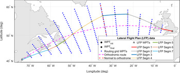
The set of LFPL candidates evaluated in the optimisation are constructed by selecting, successively, from an RGRID, the WPTs that delimit each FPL segment. First, the RGRID is constructed similarly to the method presented in ref. [Reference Dancila and Botez49] and in a flight trajectory optimisation study(Reference Dancila and Botez78) conducted by the authors. An Orthodromic Route (ORT) is constructed between WPT init and WPT final, and then divided into the minimum number of equal segments with an SLL smaller than or equal to a selected value (step size). In each ORT segment limit WPT, a new orthodrome is constructed perpendicular to the ORT (P-ORT), and new WPTs are created at locations that generate segments with a selected SLL, up to a selected maximum deviation from the ORT. The RGRID is constructed step by step, starting from WPT init. Relative to its location, the aircraft can advance to a new RGRID WPT situated one step ahead along the ORT, and a maximum number of steps (N W) along the P-ORT, on either side. Therefore, the RGRID starts with a single WPT (WPT init) and increases, at each step along the ORT, with
 $2 \times N_{\rm W}$
WPTs (N W on each side of the ORT), until it reaches the maximum deviation (number of transversal WPTs). At the other end, starting at a certain position along the ORT, the number of WPTs across the ORT starts to decrease by
 $2 \times N_{\rm W}$
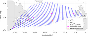
WPTs, until it reaches the final WPT (WPT final), where there is a single WPT. The candidate LFPL construction is performed step by step, starting from WPT init. For each LFPL segment, the RGRID WPTs that define the segment are selected by choosing the lateral deviation step and the number of WPTs on the segment (steps along the ORT). An illustration of an RGRID and a LFPL is shown in Fig. 1.
Example of a RGRID and a LFPL component constructed based on the RGRID.

To accelerate the flight performance evaluations, the SLL and the departure headings are computed ahead of time for each possible segment starting at a RGRID node (a maximum of
 $2 \times N_{W} + 1$
, which is the maximum number of lateral deviation choices), and stored in a RGRID node data structure. During the flight performance calculations, the segment SLL and departure heading are readily available. The distance flown by the aircraft along an LFPL segment is calculated by multiplying the segment’s SLL with a correction factor, computed based on the Earth’s radius and the aircraft’s altitude.
3.1.2 Vertical flight plan
The VFPL describes, in a concise, standardised form, the aircraft’s altitude and speed evolution along the LFPL. A VFPL can be decomposed into seven sections (flight phases): take-off, initial climb, climb, cruise, descent, approach and landing. Each VFPL section is composed of a set of segments, defined by a set of specific parameters for each segment type (e.g. the segment type, altitude, speed, position along the LFPL, etc.). Not every vertical flight trajectory segment is explicitly defined in the VFPL. There are vertical flight trajectory segments (e.g. constant altitude acceleration/deceleration, climb in cruise, etc.) that are transition segments between segments defined in the VFPL, and they are generated during the FPL accelerated flight performance calculations. In this paper, it was assumed that the WPT that demarcates two VFPL segments defines the geographic location (WPT) where the altitude/speed change is initiated (starts), and not the geographic location where the aircraft reaches the new speed and/or altitude.
Some VFPL segment parameters are implicit, ‘inherited’ from the previous segment (e.g. constant speed climb segment start altitude) or defined by the FPL (e.g. geographic location/WPT where a constant altitude and speed cruise segment ends). Other parameters are dependent on the specific context (aircraft performance, weight, atmospheric conditions, etc.) and can only be determined during the accelerated flight performance calculations (e.g. the distance necessary/geographic location where the aircraft reaches the cruise altitude).
In this study, a VFPL is considered to have three phases/sections (climb, cruise and descent) and the structure described below, similar to that used by the authors in a previous flight trajectory optimisation study(Reference Dancila and Botez78), and can contain some or all of the listed elements. The number of sections, segments, the segment types and the order in which they appear, are specific for the FPL. It is assumed that:
-
The climb is flown at [CASCLIMB, MACHCLIMB] from the initial aircraft position WPT init, at altINIT (initial aircraft altitude) to the Top of Climb (TOC; the point where the aircraft reaches the initial cruise altitude altCRZ_INIT), executed at Maximum Climb (MCMB) Thrust Lever Angle (TLA). The transition between CAS and MACH occurs at the crossover altitude;
-
The cruise phase is composed of a succession of constant speed cruise segments:
-
A constant altitude (altCRZ_INIT) and speed (MACHCRZ_INIT) cruise segment from TOC to a selected location along the lateral flight trajectory (LFPL segment);
-
A set of constant altitude and speed cruise segments ([altCRZi, MACHCRZi]) where each segment can have a different cruise altitude and/or speed value, and are delimited by selected LFPL WPTs. The set’s last segment ends at the End of Cruise (EOC – a point in cruise beyond which the aircraft is considered in descent mode, therefore no more step climbs are executed). The EOC location is selected so that the Top of Descent (TOD), the point where the aircraft starts the descent, is located after the EOC; and
-
A final constant altitude (altCRZ_FINAL – same as the altitude of the previous segment ending in EOC) and speed (MACHCRZ_FINAL) segment, from the EOC to the TOD.
-
-
The aircraft does not perform descents in cruise, i.e. the altitude for a cruise VFPL segment is always equal to or higher than that of a previous segment;
-
The descent is flown at constant scheduled speed ([MACHDESCENT, CASDESCENT]), starting from TOD, from the final cruise altitude (altCRZ_FINAL) to the final descent altitude (altFINAL) at WPT final, and executed at idle (IDLE) TLA. The transition from MACH to CAS speed occurs at the crossover altitude; and
-
The speeds (CAS and MACH) and altitudes have discrete values, multiples of 1Kn for CAS, 0.001 for MACH and 1,000ft for altitude.
The TOC and TOD locations along the LFPL are specific for the FPL data (LFPL and VFPL), aircraft performance and weight, atmospheric conditions, etc.
3.2 The aircraft performance model
The accelerated flight performance calculations were performed using a toolbox, developed in-house and based on the Base of Aircraft Data (BADA)(Reference Nuic, Poles and Mouillet21-24) version 4.0 APM developed by Eurocontrol. The BADA APM provides aircraft-specific parameters and data models (flight envelope limitations, aerodynamic and engine performance, valid aircraft configurations, etc.), and the methodology to compute the flight performance parameters of interest and the aircraft dynamics using equations based on the Total Energy Model (TEM). Specific information regarding BADA 4.0 can be obtained from Eurocontrol(22) and is subject to a license agreement.
The flight performance calculation toolbox contains a set of functions specific to each type of vertical flight trajectory segment generated for a flight along a profile defined by an FPL.
3.3 Atmospheric data model
The Atmospheric Data Model (ADM) used in this study was that presented by Dancila and Botez(Reference Dancila and Botez49). The model defines the atmospheric data, as a function of time, in RGRID nodes (see sub-section 3.1) and at a set of selected altitudes. The geographic area covered by the RGRID, the range of altitudes selected for the vertical flight profile, and the time domain estimated to cover the possible flight times between the initial and final WPTs determine the atmospheric data prediction files to be retrieved from the meteorological service agency. This ADM has the advantage that, in a large majority of the cases, the atmospheric parameters used in the flight segment performance calculations only require 1D linear interpolations to compute their values in an RGRID node, at the altitude and time instance of interest. The ADM was shown(Reference Dancila and Botez49) to be on average six times faster, and as accurate as when computed by linear interpolations from the GDPS GRIB2 data. Atmospheric data at points other than the RGRID nodes, a reduced number of occurrences during the flight performance calculations (e.g. at the final points of climb/descent and acceleration/deceleration segments), can be computed through linear interpolation based on the atmospheric data in the grid nodes. Depending on the specific case, a smaller number of interpolations may be required than when the GRIB2 data is used.
3.4 Accelerated flight simulation and flight performance parameters calculations
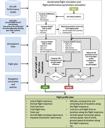
The accelerated flight simulation performs a step-by-step simulation of the aircraft’s evolution along the flight trajectory determined by the selected FPL. The specific methodology employed for performing the accelerated flight simulation, used for flight trajectory prediction and optimisation, is described in ref. [Reference Schreur50] and illustrated in Fig. 2.
Accelerated flight simulation and flight performance parameter calculations.

The simulation is performed phase by phase, starting from the initial aircraft position (geographic location, altitude and time), attitude (banking angle, climb/descent angle, etc.), speed and aircraft configuration (weight, fuel quantity, etc.). For each flight phase, the accelerated simulation successively estimates the aircraft’s evolution along each VFPL section and LFPL segment. Each VFPL segment is decomposed into a set of sub-segments, chosen so that the mathematical model that describes the aircraft and the performance parameters’ evolution does not change, and is then divided into smaller sub-segments (integration steps). The parameter along which the decomposition is made (altitude, distance, time) is a function of the segment’s type. The integration step size is chosen as a trade-off between computation time and precision. Small integration steps increase the results’ accuracy, but the computation time may become prohibitive.
For each sub-segment, the flight performance parameters are computed by multiplying the parameter values computed in a point on the sub-segment with the integration step size. The computed data are then used to determine the aircraft’s weight, position along the LFPL, altitude, speed, etc., at the segment’s end. These data are the initial conditions for the next sub-segment’s accelerated simulation. During the accelerated flight simulation, new flight trajectory segments are created that do not have their correspondent in the VFPL segments. They are transitions between VFPL segments, such as acceleration/deceleration segments between two consecutive constant speed segments or climb/descent segments between two constant altitude cruise segments.
The simulation starts by performing the climb phase accelerated simulation, from WPT init to the TOC, followed by the cruise phase simulation, from the TOC to the EOC. Next, the descent phase accelerated simulation is conducted backwards (backward integration), from WPT final to the TOD. The aircraft weight and crossing time at WPT final are estimated heuristically, based on the aircraft’s weight and crossing time at the EOC. After the descent phase simulation, the estimated aircraft position, weight, and crossing time at the TOD are known. Finally, the cruise segment between EOC and TOC is simulated, and the aircraft weight and crossing time at the TOD are known, based on the forward simulation from the initial waypoint. The heuristic estimation of the aircraft weight and crossing time at WPT final is validated by comparing the differences between the aircraft weight and crossing time at the TOD, computed forward, from the cruise phase, and those computed backwards, from the descent phase. If the difference(s) is (are) larger than selected threshold(s), they are applied as corrections to the estimated values at WPT final. The simulation from the EOC to WPT final and the validation are repeated until the simulation converges (the differences are smaller than the thresholds) or the number of iterations surpasses a selected maximum value (simulation error).
During the simulation, for each sub-segment, the flight parameters are validated relative to the flight envelope limitations and fuel requirements (if the flight requires more fuel than available). An accelerated flight simulation module option allows, if desired, the correction of FPL segments that would result in flight parameters outside the aircraft’s flight envelope (invalid altitude – speed profiles). The corrected FPL (with valid altitude – speed profiles) is returned by the accelerated flight simulation function for future use in the optimisation.
3.5 The proposed optimisation method
The proposed optimisation method uses a new evolutionary search method, derived from the NSGA-II. The first sub-section (3.5.1) presents the general considerations and observations regarding the optimisation problem. Sub-section 3.5.2 presents the characteristics of the candidate FPLs solutions selected and evaluated during the optimisation. Next, sub-section 3.5.3 presents the genetic operations applied to candidate FPLs (crossover and mutation) and, finally, sub-section 3.5.4 details the proposed method.
3.5.1 General considerations
For a selected FPL, a change in total flight time can be obtained by changing one or more FPL parameters, for one or multiple segments. Given that the candidate FPL parameters (speeds, altitudes, WPT locations) have discrete values, the set of obtainable flight times are also discrete values. The complex and non-linear relationship between (lateral and vertical) FPL parameters, atmospheric conditions and the flight parameters of interest (total flight time and total fuel burn), as well as the atmospheric conditions which vary as a function of the selected altitude, route and the time when the aircraft crosses each trajectory point, makes it possible that for each RTA value the optimal solution is located in a different search space region.
The proposed method is based on the following observations:
-
The fuel burn variation versus flight time cannot be estimated a priori. Depending on the specific optimisation problem, the fuel burn variation in general, and specifically for the optimal (minimum fuel) solution set, could increase or decrease with the flight time, or it may not have a monotonous variation;
-
The optimisation problem can be seen as a constrained MOO with a two-dimensional objective space (fuel burn versus flight time); however, this is not a classical MOO problem since the set of optimal FPL solutions might not form a Pareto front (see the first observation). The solutions sought here do not constitute a trade-off between fuel burn and flight time, but they are the FPLs that yield the minimum fuel burn for the set of RTA constraints;
-
Techniques and elements from the MOO methods can be adopted for solving the optimisation problem: population-based search methods (EAs), tentative solution (TS) set, ranking and fitness assignment for the evaluated solutions at a search iteration, searches performed in the objective space, etc.; and
-
The differences relative to classic MOO methods would have to address the population elements’ ranking and their fitness value assignment, which guides the selection of population elements for the genetic operations and, therefore, the search.
3.5.2 The set of candidate flight plans
The RGRID and the set of candidate FPLs (composed of LFPLs and VFPLs) conform to the models presented in sub-section 3.1. Ideally, the range of altitudes and speeds from which the altitude/speed pairs that define the VFPL segments are chosen to cover the entire flight envelope, without extending beyond it. FPLs that have segment parameters outside the aircraft’s flight envelope or require more fuel than available reduce the search efficiency, as they spend computational resources without adding information that could guide the search. Given the complexity/impossibility to determine a priori, at WPTs along the flight trajectory, the parameters (aircraft’s weight, atmospheric conditions, etc.) that determine the aircraft’s flight envelope limitations, and to ensure that the entire flight envelope is covered, the range of speeds and altitudes for the VFPL segments were chosen as follows:
-
CAS for climb (descent): CAS INIT (CAS FINAL) to VMO – 10Kn;
-
Climb (descent) MACH: MACH equivalent for CAS INIT at alt INIT (CAS FINAL at alt FINAL) to maximum operational MACH speed limit (MMO) – 0.01;
-
Cruise altitudes are multiples of 1,000ft, between a selected minimum cruise altitude and the service ceiling for the aircraft model; and
-
Cruise speeds are multiples of 0.001 MACH, between a minimum selected value and MMO – 0.01.
At the beginning of the flight, when the aircraft is heavier, the range of valid cruise altitude and speed combinations are smaller than for the other flight segments. Therefore, the set of alt CRZ_INIT and MACH CRZ_INIT combinations are determined heuristically, as the valid combinations of altitudes multiples of 1,000ft and speeds multiples of 0.001 MACH for an aircraft weight resulted after a climb at 250Kn, from alt INIT to the minimum initial cruise altitude.
3.5.3 Flight plan genetic operations
Due to their different structures, the LFPL and the VFPL genetic operations are different. The first sub-section presents the genetic operation applied to LFPLs, and the second sub-section presents the genetic operations applied to VFPLs.
3.5.3.1 Lateral flight plan genetic operations
The LFPL genetic operations are applied in an LFPL WPT selected at random, between the second and the second-to-last WPT. Performing a crossover at the first or last WPT would not yield new FPLs, and mutations cannot be performed at these locations. If, at the location where the crossover must be performed, the difference between the lateral deviations for the two LFPL WPTs is larger than the maximum lateral deviation step, the crossover cannot be obtained just by swapping the final LFPL sections. A transition section is constructed, so that at each step along the ORT the lateral deviation relative to the previous WPT is less than or equal to the maximum lateral deviation step size. An LFPL mutation changes the lateral deviation for the WPT situated at the selected location, relative to the previous WPT, to a new value within the range of possible relative lateral deviations. For the following WPTs, the deviation relative to their preceding WPT is maintained, and limited to the RGRID.
3.5.3.2 Vertical flight plan genetic operations
The crossover between two VFPLs is applied in the cruise section, at points that delimit cruise segments, between the WPT at the end of the initial cruise segment and the EOC. The crossover can be performed on the speed component, the altitude component or on both. The VFPL speed component crossover is obtained by swapping the final sections of the VFPL speed component (between the crossover position and the end of the VFPL). A VFPL speed component mutation can be performed on any segment by changing the selected segment’s speed to a value within the range allowed for the segment (see sub-section 3.5.2). If at the point where the VFPL altitude component crossover is performed the altitudes are identical, the crossover swaps the final sections (from the crossover position to the end of the VFPL) between the two VFPLs. If the altitudes are different, given that the descent in cruise is not accepted, for the VFPL with the higher altitude at the crossover position the swap is performed at a further location, where the altitude on the other parent profile is equal or higher (if it exists). For the FPL with a lower altitude, the swap is performed at the crossover location. The mutation is obtained by modifying the cruise altitude of a randomly selected cruise segment. The new altitude is selected from the range of altitudes considered for that segment. The altitudes for the cruise segments that follow are modified, if necessary, to be equal to or higher than the selected new altitude (no descent in cruise).
3.5.4 Search method description
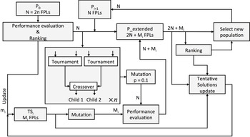
The proposed method uses an EA, based on GAs, derived from the NSGA-II algorithm(Reference Deb, Pratap, Agarwal and Meyarivan72). The differences between the proposed method and the NSGA-II method presented in(Reference Deb, Pratap, Agarwal and Meyarivan72) consist in the methods used for non-dominance/ranking determination, the fitness assignment for crossover element selection, the TS set construction and update, and its propagation to the extended population. In the proposed method, the tentative set size is equal to the number of RTA constraints and is initially empty. Each TS set member is associated with an RTA constraint. In each iteration, a population member that yields a flight time within an RTA constraint bounds will replace the tentative solution element for that RTA if the fuel burn is lower, and will not affect the other TS set members. A high-level block diagram representation of the proposed search method is shown in Fig. 3. A detailed description is presented in the paragraph below.
Proposed search method block diagram.

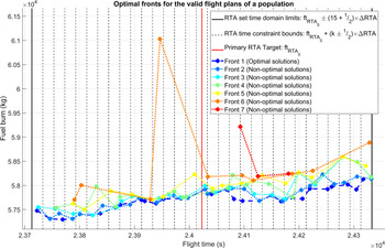
An initial population (P0), with N elements, is randomly created according to the RGRID, LFPL and VFPL templates, and the parameter value ranges for each FPL component. The initial population FPLs are evaluated, and the fuel burn and flight times are calculated. During the accelerated flight simulation of the first population, the FPLs that are invalid relative to the aircraft’s flight envelope are corrected and updated in the population, so that the search starts with the largest number of valid candidate solutions and, therefore, better information to guide the search. For invalid FPLs (caused in the first population by FPLs that require more fuel than available and, for the next populations also due to aircraft envelope limits violation), the fuel burn and flight time are assigned penalty values, larger than for any valid FPL. The range of flight times between the initial and final points that cover the entire set of possible flight times along the set of candidate FPLs are estimated heuristically. In the next step, the population elements are evaluated relative to the RTA values and fuel burn, and assigned ranking and fitness. Similar to the method proposed by Jensen(Reference Jensen73), the population elements’ ranking is performed by first sorting the population based on the two cost function components (first by flight time, and then by fuel burn), and then assigning them to optimal fronts (sets of population elements with the same ranking/level of optimality). The elements of the ordered list that have a flight time within the RTA constraint bounds of an RTA value are successively retrieved, ordered as a function of fuel burn, and then ranked. The element with the lowest fuel burn is assigned rank 1 (assigned to front 1), the next is assigned rank 2 (assigned to front 2) and so on. The best element for the RTA constraint value (the element having rank 1) is copied to the TS set. The uniform distribution of the solutions along the optimal front results from the rank assigning method. The non-valid population elements (those that have a flight time outside the RTA constraint set bounds or are invalid) are assigned the lowest rank (highest rank value) and form the last/least optimal front.
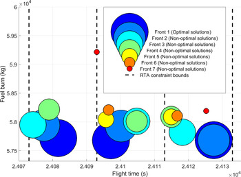
An example of fronts (solutions with the same ‘level of optimality’) for an FPL population is shown in Fig. 4 (the last front, corresponding to non-valid FPLs, is not represented). It can be noted that, for the case represented in Fig. 4, the tentative optimal solutions are present for every target RTA constraint. However, the number of non-optimal solutions and their quality (fuel burn value relative to the optimal solution for the RTA constraint) differ for each RTA. In general, the presence in a population of an optimal solution for an RTA constraint, its performance relative to the global optimum and the number of non-optimal solutions are a function of the evolution of the search process.
Example of solution fronts for a population (the image does not show the last front: the non-valid FPLs).

Figure 5 gives a detailed view of three adjacent RTA constraints represented in Fig. 4 and delimited by the time interval (24073 24133] seconds. It can be noticed that some solutions from adjacent fronts could be very close: e.g. the tentative optimal solution (front 1) and the next, near-best solution (front 2) for the RTA constraint bounded by the time domain (24113 24133] seconds. The choice to assign different sizes for the dots that represent solutions from different fronts was determined by the fact that, in such cases, dots of identical size would overlap, rendering some solutions not visible.
Example of valid solutions in a population: detailed view of the RTA constraints from Fig. 4 delimited by the interval (24073 24133] seconds.

In the next step, an extended population (P_extended) is created by copying the current population’s N elements, then by adding N elements generated by N/2 crossover operations, followed by a mutation with probability p = 0.1 – in a similar manner to the NSGA-II method. The difference is that, in the proposed method, the Mi non-empty TS set members are mutated and added to the extended population (a local search).
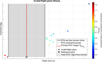
The selection of population elements for crossover is performed at random. Four different elements are selected and compared two by two. If the two elements have different ranks, then the element with the lowest rank (highest fitness) is selected as a ‘parent’. If the elements have the same rank and are valid FPLs, then the element with the smallest number of elements within the RTA constraint bounds is selected. If they both have an identical number of elements within the RTA bounds, the FPL with the lowest fuel burn is selected. If the fuel burn is also identical, the FPL with a flight time closer to the RTA constraint is selected. If the FPLs also have the same flight time difference relative to their respective RTA constraints, the parent is randomly selected among the two. If the two elements have the same rank and are non-valid, the parent is selected based on the Euclidian distance, in the normalised objective space, between the element’s projection on the normalised objective space, and a reference point with coordinates corresponding to the minimum fuel burn obtained for the population and the central RTA constraint value (RTA0). The element with the smallest distance to the reference point is selected as a parent. If both elements have the same distance, then the element with the lowest fuel burn is selected. If the fuel burn is also identical, the parent is selected at random between the two elements. An illustration of the fitness values for non-valid FPLs, expressed as the Euclidian distance to a reference point in the normalised objective space, is given in Fig. 6. Here also the number of invalid FPLs and their fitness are a function of the evolution of the search process. In the example shown in Fig. 6, the best-fit invalid FPL (the dark-brown dot) is located near the minimum RTA constraint set bound and has a low (normalised) fuel burn. The least-fit FPL is the dark-blue dot, located in the upper right corner of Fig. 6, which has the largest fuel burn and flight time, and is the farthest from the reference point.
Example of fitness for the non-valid FPLs of a population, calculated based on the Euclidian distance, in the normalised objective space, between the FPL’s projection and the reference point.

The children elements, the new extended population members, are generated by crossover between the two winning parents, where the crossover is performed on the lateral or vertical FPL component, selected at random.
The subsequent step is similar to that of the NSGA-II method. The new elements in the extended population are evaluated, and the extended population is ranked and assigned to optimal fronts. If the extended population contains mi elements that are new solutions (for RTA constraints with empty Tentative Solution element) or better solutions (lower fuel burn than the Tentative Solution element), then the mi solutions update the TS set. The new population (P1), for the next iteration, is composed of the best N elements from the extended population – as in the NSGA-II method. The copied elements are retrieved, successively, from the optimal fronts associated with the ‘extended population’, starting with the optimal front elements (rank 1), and continuing with the elements from the subsequent, less optimal fronts (higher ranks), until N elements are retrieved. If the remaining number of elements to be retrieved, N R, is less than the number of elements in the current front, then the first N R elements are copied from the front. The steps listed above are repeated until the selected number of iterations is reached. The TS set at the end of the optimisation is the set of optimal solutions. Given the randomness associated with GAs and the flight trajectory optimisation problem characteristics, the solution set could contain solutions for all RTA constraints, for some, or for none, and the solutions may be optimal, near optimal or not optimal.
The impacts of different possible changes in the proposed method are evaluated using seven method variants. The first variant is the one described above. The other six variants differ as follows:
-
Non-valid FPLs’ fitness assigned based on the absolute time difference to the central RTA constraint (RTA0) – not the Euclidian distance to the reference point;
-
The extended population does not include mutated TS set versions (local search);
-
Non-valid FPLs’ fitness assigned based on the absolute time difference to the central RTA constraint (RTA0), and the extended population does not include mutated TS set versions (local search);
-
The extended population is created by crossover applied on both LFPL and VFPL;
-
The initial population FPLs are not corrected relative to the aircraft flight envelope; and
-
Different number of iterations used in the optimisation.
4.0 RESULTS
This section presents the results of tests performed to evaluate the performance of the proposed FPL optimisation method. First, sub-section (4.1) presents the test environment used in the evaluation. Then, sub-section 4.2 describes the test scenario used to perform the evaluation. Sub-sections 4.3 and 4.4 present the research questions investigated in this study and the test cases devised for this purpose. Finally, sub-section 4.5 presents and discusses the results.
4.1 Simulation environment
The proposed method was evaluated on a PC-based platform with a 2.8GHz AMD Phenom II X4 B93 processor, 8 GB of RAM and Windows 10 Enterprise, using code developed in MATLAB (R2108a). The flight performance parameters for candidate FPLs were calculated using a module developed in-house, in MATLAB, based on the Boeing 777-300ER BADA 4.0 APM published by Eurocontrol.
4.2 Test scenario
The test scenario was the optimisation of a flight section that starts in climb, at 10,000ft and 250Kn CAS, and ends in descent, at 10,000ft and 250Kn CAS. The aircraft was considered to be in normal operation (no malfunctions) and in clean configuration (retracted landing gear, flaps and spoilers). The aircraft weight and fuel at the initial point were taken to be 0.5 and 0.7, respectively, of their maximum allowed values for the aircraft model. For a ‘realistic’ evaluation (attainable constraint times for the selected flight section, atmospheric conditions and aircraft model), the initial and final FPL points and their crossing times were recovered from real flight track data, retrieved from the FlightAware website (www.flightaware.com). The selected flight was American Airlines AAL107(79), between London Heathrow (LHR) and New York John F. Kennedy (JFK) airports, flown on February 25, 2019, chosen at random from the flights performed that day with the same aircraft model as the aircraft performance model available to the authors.
Currently, the North Atlantic traffic observes specific navigation policies, and the aircraft follow predetermined tracks: the North Atlantic Organized Track System (NAT-OTS). This study/proposed method assumes possible future navigation paradigms, such as TBO or free flight, where the aircraft can fly along the FPL/trajectory that is best suited for the mission (aircraft type, load, atmospheric conditions and departure–destination pair).
The reference points and the crossing times were selected as the track data points, in climb and descent, where the aircraft was closest to the altitude of 10,000ft:
-
Initial point (WPT init): Lat. 51.5144 N, Lon. 1.0188 W, Time 12:27:50 EDT; and
-
Final point (WPT final): Lat. 40.3386 N, Lon. 73.8018 W, Time 19:07:28 EDT.
The set of N adjacent RTA constraints were calculated based on the aircraft’s crossing time at WPT final, considered as the primary RTA constraint (RTA 0), defined by RTA values within a range of RTA0 ± 5min (
 $RTA = RTA_{0} + k \times \Delta RTA$
, with
 $k \in \mathbb{Z}, -15 \le k \le 15 $
), and window width ΔRTA = 20s. This produced 31 RTA constraints, and therefore, the optimisation was expected to produce 31 optimal FPLs, one for each RTA value. The RTA constraint bounds were selected as follows:
 \begin{equation}\begin{cases}\begin{array}{c@{\quad}l}\bigg[RTA_{0}+\left(k-\dfrac{1}{2}\right)\times \Delta RTA, RTA_{0}+\left(k+\dfrac{1}{2}\right)\times \Delta RTA\bigg)& k<0\\[12pt]\left[RTA_{0}- \dfrac{1}{2}\Delta RTA, RTA_{0}+\dfrac{1}{2}\Delta RTA\right] & k=0\\[12pt]\bigg(RTA_{0}+\left(k-\dfrac{1}{2}\right)\times \Delta RTA, RTA_{0}+\left(k+\dfrac{1}{2}\right)\times \Delta RTA\bigg] & k>0\end{array}\end{cases}\end{equation}
The set of RTA values at WPT final were transformed into total flight time constraints, calculated as a difference, in seconds, between the RTA at WPT final and the aircraft crossing time at WPT init:
 \begin{equation}ft_{RTA_{n}}=\left(RTA_{n}- t_{WPT_{init}}\right)\times 3600\end{equation}
where
-
 $ft_{RTA_{n}}$
is the total flight time constraint for the nth RTA (RTAn); and
-
$t_{WPT_{init}}$
is the aircraft crossing time at WPT init.


The value obtained for
 $ft_{RTA_{0}}$
was
 \begin{equation}\begin{array}{ll}ft_{RTA_{0}}&=RTA_{0}-t_{WPT_{init}}=t_{WPT_{final}}-t_{WPT_{init}}\\[6pt]& =19h\ 07 \mathrm{min}\ 28s-12h\ 27 \mathrm{min}\ 50s=6h\ 39\mathrm{min}\ 38s=24023s\end{array}\end{equation}
The set of flight time constraints were obtained by replacing RTA0 with
 $ft_{RTA_{0}}$
in Equation (1).
The selected RGRID parameters were a maximum ORT sub-segment SLL of 50NM, a maximum lateral deviation of 500NM from the ORT, a lateral deviation step of 10NM and a maximum of two lateral deviation steps that can be performed at one time. The resulted RGRID (Fig. 7) has the ORT divided into 60 equal sub-segments with an SLL of 49.71NM, and a maximum of 50 deviations (WPTs) on each side of the orthodrome.
The RGRID for the set of LFPLs evaluated for the flight AAL107(79) optimisation.

The parameters selected for the candidate VFPLs were:
-
Climbs at constant [CAS, MACH] and MCMB TLA: [250 to VMO – 10] Kn CAS, and [0.452 (250Kn CAS at 10,000ft) to MMO – 0.01] MACH;
-
Descents at constant [CAS, MACH] and IDLE TLA. Speed ranges as for climb;
-
Climb in cruise performed at constant MACH, MCMB TLA, and 500fpm climb rate;
-
Accelerations in cruise performed at maximum cruise (MCRZ) TLA and decelerations at IDLE TLA;
-
The sets of valid initial cruise altitude and valid cruise speeds are determined heuristically (see sub-section 3.5.2);
-
A constant altitude (initial cruise altitude) and MACH speed (initial cruise MACH speed) from the TOC to the eighth LFPL WPT (approx. 400NM from WPT init);
-
EOC is placed at the 53rd LFPL WPT (approx. 400NM before WPT final);
-
From the eighth LFPL WPT to the EOC, the cruise section defines constant altitude and speed segments with a length of approximately 250NM (five LFPL segments). The cruise altitude and/or speed changes can occur at the LFPL WPTs [8, 13, 18, 23, 28, 33, 38, 43, 48]; and
-
The cruise phase altitude and speed values and the MACH speed for the final cruise segment (from WPT 53 to TOD) are selected at random: altitudes between 28,000ft and 43,000ft, and speeds between 0.68 and 0.9 MACH.
Next, the ADM was constructed based on the RGRID, the range of VFPL altitudes, and the time domain that covered all flights along the candidate FPLs. The maximum flight time for a flight between WPT init and WPT final was assumed to be 10h 00′ 34′′ (
 $1.5 \times ft_{RTA_{o}}$
). Therefore, the time domain of interest for the atmospheric data is
 \begin{equation}ft_{domain}=\left[t_{WPT_{init}},t_{WPT_{init}}+1.5\ ft_{RTA_{0}}\right]=[12:27:50, 22:28:24]EDT\end{equation}
The population size for the algorithm implementing the proposed method was selected to be 62, twice the number of searched FPL solutions. Given the proposed method’s stochastic nature, ten test runs were conducted for each optimisation method variant.
4.3 Research questions
The research questions evaluated in this study are:
-
Does the optimisation method identify solutions for all RTA constraints?
-
How fast (in what generation) does the first tentative solution for an RTA value appear?
-
What is the fuel burn difference between a ‘random’ FPL that satisfies the RTA constraint (the first identified tentative solution) and the final solution?
-
How many iterations are necessary until a tentative solution reaches a fuel burn that is 1%, 0.1%, 100kg and 50kg over the final solution, or the final solution?
-
How different are the solutions identified in the ten test runs of a test case?
-
Does adding mutated tentative solutions to the extended population (local search) improve the results?
-
Does a FPL correction relative to the flight envelope, in the initial population, improve the results?
-
How does the method’s performance change if the extended population is generated by crossover solely on the LFPL or VFPL (chosen at random), or on both?
-
What is the effect of assigning the fitness value for non-valid FPLs as a function of Euclidian distance to a reference point versus the absolute time difference relative to the primary flight time constraint
$\ ft_{RTA_{0}}$
? -
Does an increase of the number of iterations (generations) improve the results?
-
What are the differences between an optimisation performed for 300 generations versus one performed for 1,000 generations?

4.4 Test cases
A test case configuration synopsis of the optimisation method variants is presented in Table 1.
Test case configuration synopsis

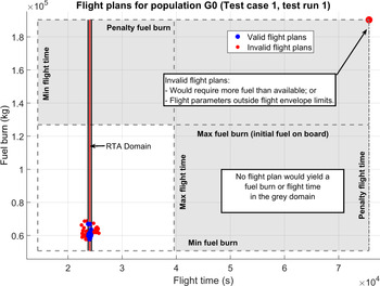
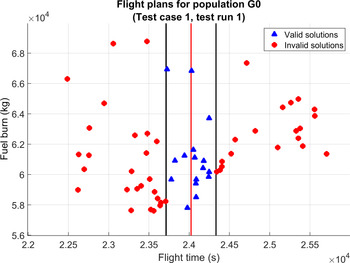
For an invalid FPL, the flight time and fuel burn were assigned penalty values:
 $ 3 \times ft_{RTA_{0}}$
for the flight time, and 1.5 times the initial fuel quantity for fuel burn (see Fig. 8).
Initial population (G0) represented in the objective space (fuel burn – flight time) for test case 1, test run 1.

In the first population, where all the FPLs are generated at random, one, multiple or all FPLs may be non-valid. Since all invalid FPLs have the same values for fuel burn and flight time, this could affect the algorithm’s ability to properly guide the search. For test cases 1–5 and 7, the invalid FPLs in the initial population were corrected (see sub-section 3.4). For test case 6, the invalid FPLs in the initial population were not corrected, to evaluate their influence on results.
4.5 Results and discussion
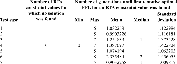
The number of invalid profiles in the initial generation when the FPLs were corrected (test cases 1–5 and 7) was between 0 and 3 (4.84%). For test case 6, the number of invalid FPLs was between 19 and 24 (30.65–38.71%). However, over the entire set of 70 test runs, the first population (G0) contained tentative solutions for a minimum of 2 and a maximum of 20 RTA values (mean 11.27, median 12, standard deviation 3.937). Moreover, for all test cases, test runs and RTA values, the first tentative solution appeared after a maximum of eight generations (Table 2). Therefore, in all test cases, by the eighth generation a complete TS set was found and, as a result, the final solution contained optimal FPLs for all RTAs. Table 2 presents the statistical data for the first RTA value tentative solution occurrence.
Flight plan solution occurrence for an RTA constraint value

The results show that the invalid FPLs generated in the first population do not have a large impact on the ability to obtain, within the first few iterations, tentative FPL solutions for all the RTA values. An illustration of the FPLs generated in the first population for test case 1–test run 1, represented in the objective space (fuel burn versus flight time), is given in Fig. 8. Among the 62 randomly generated initial FPLs, 16 were valid (the blue dots in Fig. 8), and 46 were non-valid (the red dots in Fig. 8). Among the 46 non-valid FPLs, one required more fuel than available (the red dot in the upper right corner of Fig. 8). A more detailed illustration, for FPLs with parameters within the aircraft’s flight envelope, is given in Fig. 9.
Initial population (G0) FPLs represented in the objective space, (flight parameters within the aircraft’s flight envelope) for test case 1, test run 1.

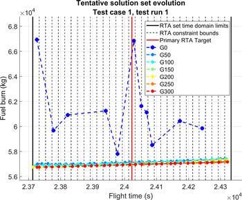
Figure 10 shows an example of global optimisation evolution obtained for test case 1–test run 1. The initial population (G0) yielded only 11 tentative solutions, with a fuel burn difference relative to the final solutions (optimal solutions for the same RTA values at G300) between 10192.47kg (17.961%), for RTA
 $ft_{RTA_{0}} -15 \times \Delta RTA$
, and 887.45kg (1.559%), for RTA
 $ft_{RTA_{0}} -2 \times \Delta RTA$
. At the 50th generation (G50), the differences were found to be between 262.56kg (0.462%), for RTA
 $ft_{RTA_{0}}-13 \times \Delta RTA$
, and 167.84kg (0.295%), for RTA
 $ft_{RTA_{0}}-5 \times \Delta RTA$
.
Example of global TS set evolution for test case 1, test run 1.

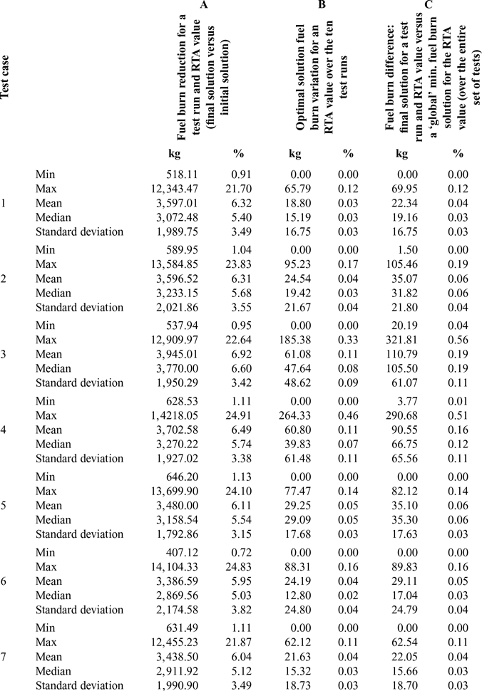
The results presented in Table 3, column A, show a synopsis of the fuel burn reduction between the initial, random, tentative solutions and the optimal FPLs at the end of the optimisation. The seven method variants (test cases) yielded similar results. These results are influenced by how far the random initial population (G0) candidate FPLs are from the optimal solutions. Column B of Table 3 shows how close (in terms of fuel burn) are the optimal solutions found for ten runs of an identical test case and RTA value. The worst results (the maximum difference between test run results, and the maximum variance) were obtained for the test cases 3 and 4, where no local search was performed. The best results were obtained for the optimisation method variants 1 and 7, where the initial population’s invalid FPLs were corrected, a local search was performed and the fitness for the non-valid FPLs was computed using the Euclidian distance to the reference point. Among the two (test cases 1 and 7), the best results were obtained for test case 7, when the optimisation was performed for 1,000 iterations.
Synopsis for the optimisation results obtained using the proposed method

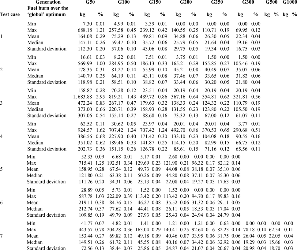
Column C of Table 3 shows the results of a comparison between the optimal FPL fuel burn for an RTA value and a test run, with the ‘global optimum’ for the RTA value (the best fuel burn for the RTA value obtained from the 70 test runs – the 10 test runs for each of the seven test cases). Once again, the best results were obtained for the test cases 7 and 1, with maximum fuel burn differences relative to the ‘global optimum’ of 62.54kg (0.11%) and 69.95kg (0.12%), respectively.
The worst results were obtained for test cases 3 and 4, with maximum fuel burn differences of 321.81kg (0.56%) and 290.68kg (0.51%), respectively. It can be concluded that the local search significantly improves the optimisation results. The improvement is obtained at the expense of computation time; the extended population increases by up to 31 elements, and therefore, a higher number of flight performance calculations must be conducted.
Comparing the results obtained for test cases 1 and 2, where the only difference between the two test cases is the fitness assignment method for the non-valid FPLs, it can be seen that test case 1 yields better results. The maximum fuel burn difference relative to the global optimum for an RTA constraint for the test case 2 is larger with 35.51kg (0.07%) than that obtained for the test case 1. It can be concluded that the non-valid FPL fitness calculation based on the time difference to a reference point, although easier to implement and less computationally expensive, degrades the optimisation results. A comparison between the results obtained for test cases 1 and 5 shows that the results obtained for test case 1 (crossover is performed on only one component of the FPL) are better both in terms of maximum difference between the results for ten identical test runs and the maximum fuel burn difference relative to the ‘global optimum’. A comparison of the results obtained for test case 6 and test case 1 shows that correcting the invalid initial candidate FPLs, generated randomly for population G0, improves the optimisation results.
An illustration of a tentative solution evolution for an RTA value (test case 1, test run 1,
 $ft_{RTA_{0}} -13 \times \Delta RTA$
) is given in Fig. 11:
-
The first tentative FPL solution appeared in the second generation (G2);
-
A fuel burn value equal to 1% higher than the final solution (G300) was achieved in G10;
-
Less than 0.1% over the fuel burn for G300 was reached at G145;
-
Less than 100kg over fuel burn at G300 was reached at G119;
-
Less than 50kg over fuel burn at G300 was reached at G145; and
-
The final solution was reached at G161.
Example of tentative FPL solution evolution for test case 1, test run 1, and RTA constraint value
 $\boldsymbol{ft}_{\boldsymbol{RTA}_{\textbf{0}}} - \textbf{13} \boldsymbol\times \boldsymbol\Delta \boldsymbol{RTA}$
.

The final solution uses 1435.40kg (2.466%) less fuel than the initial tentative FPL solution.
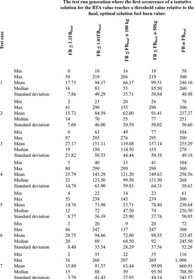
Table 4 presents the number of iterations until the tentative FPL solutions reached a selected threshold relative to the final solution fuel burn. For each test case, the analysis is performed over the ten test runs and for the entire set of RTA values. In this case too, the optimisation method versions 3 and 4 (test cases 3 and 4) yield the worst results among test cases 1–6, in which the optimisation was performed for 300 generations. The results suggest that test case 7 yields the worst results (converges after a large number of iterations). However, the optimisation was performed for 1,000 iterations (3.3 times more than for test cases 1 to 6), and therefore, new tentative solutions appear late in the optimisation, beyond the 300th iteration.
Number of algorithm iterations until the tentative solution reaches a fuel burn (FB) below a threshold value relative to the final solution (FBfinal)

A comparison of the results in column C, between cases 1 and 7, reveals that the maximum fuel burn reduction relative to the general optimum (7.41kg, or 0.01%) may not justify the additional 700 iterations. The results obtained for test cases 1, 2, 5 and 6 are close, and suggest that test case 1 converges faster to the selected threshold fuel burn values (except for 100kg over the final solution fuel burn, where it performed the worst).
Table 5 presents the fuel burn reduction, relative to the ‘global’ optimum, at different points (iterations) during the optimisation. Test cases 1 and 7 have identical optimisation method configurations, except for the number of iterations. For an FPL solution at the 300th iteration, the maximum fuel burn differences relative to the ‘global’ optimum for an RTA value are different (a difference of 12.28kg or 0.02%), due to the optimisation method’s stochastic nature (due to the randomness characteristic for EAs).
Synopsis of the fuel burn improvement for the tentative FPL solution for the set of RTA constraints, relative to the ‘global’ optimal solutions, at a set of points (iterations/generations) during the optimisation

Together, the results for test cases 1 and 7, at the 300th iteration, are equivalent to running test case 1 for 20 times. As such, relative to the ‘global’ optimal solutions, variant 1 of the optimisation method found solutions that had a higher fuel burn: between 0kg and 82.23kg (0.14%), with a mean of 27kg (0.04%), a median of 23.58kg (0.04%) and a standard deviation of 19.37kg (0.03%). These results confirm that test case 1 still produced the best results; however, they are just marginally better relative to results obtained for test cases 5 and 6.
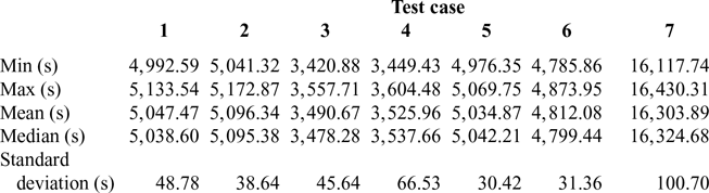
The execution times for the tests performed in this paper are presented in Table 6. These are total execution times, from the start of the optimisation (initialisations), and include loading the aircraft performance model and the reference track data, processing the reference track data, RGRID construction, loading the atmospheric data and storing the large amounts of data needed to analyse the evolution and the performance of each test run.
Execution times obtained for the seven variants (test cases) of the proposed optimisation method

The execution times are affected by the fact that the code was written in MATLAB (interpreted code) in a Windows environment (the processor time for a task is allocated by the operating system according to its own priorities), with large data structures stored in the memory.
A comparison of the execution times between test cases 1 and 3, and 2 and 4, shows that the local search performed during the optimisation increased the execution time by approximately 1,568.39–1,591.89s (an increase of close to 30%), which was expected. As more tentative FPL solutions for the RTA constraint set are identified, mutated and added to the extended population set, more FPL performance calculations must be performed (93 FPL evaluations in every iteration, in comparison with 62 FPL evaluations if the local search is not performed). The local search produced a maximum reduction in fuel consumption of between 250kg (test case 1 versus test case 3) and 185kg (test case 2 versus test case 4) (see Table 3 column C). The effect of generating the extended population FPLs through crossover on both lateral and vertical FPLs (test case 5) was an increase in execution time by a maximum of 36s and did not yield better results. This result could be due to the specifics of the FPL components’ crossover, and to the fact that performing a crossover on both the LFPL and VFPL components produces child FPLs that are too different from the parents, and thus results in a loss of good genetic information. The invalid FPL parameters’ correction (test cases 1 versus 6) resulted in a maximum increase in execution time of 260s and reduced the maximum fuel burn difference with respect to the reference profile by 20kg. Finally, increasing the number of optimisation iterations beyond 300 (test case 7 versus test case 1) did not produce significantly better solutions; however, for the 1,000 iterations performed for test case 7, the execution time increase was of approximately 11,300s, or 220% more than for test case 1.
5 CONCLUSION
This paper presents a new optimisation method that addresses a flight planning problem where the flight planner/DM has a preferred time domain for an aircraft crossing time at a WPT or they must include an RTA constraint. The proposed method was able to quickly identify, within the first eight iterations, tentative solutions for the entire set of 31 selected RTA values. These initial tentative solutions are not optimal; they are random FPLs that satisfy the optimisation objective’s time constraint (not the minimum fuel requirement). Seventy test runs were conducted for the same optimisation problem (ten runs for each optimisation method variant). The best solutions (FPLs that yield the minimum fuel burn) for each of the 31 RTA values were considered the ‘global’ optimums and were used as references, to evaluate the performance of the proposed method and its variants (i.e. the influence of various techniques applied during the optimisation, such as adding a local search).
The tests showed that, relative to the initial, random, tentative FPL solutions, the optimisation method can yield a fuel burn reduction of up to 14,000kg, depending on how far from the optimum profile the initial FPL is. Although a local search performed in each iteration increases the execution time by 30%, it also increases the solution’s quality, both in terms of reduction of the maximum fuel burn variation between FPL solutions for two runs of the optimisation, and in a reduction of the maximum fuel burn difference relative to the ‘global’ optimum, from 321kg to 69kg (a better convergence to a ‘global’ optimum). Performing a correction of the invalid FPLs in the initial population improves the solution quality, with a relative minimal increase in execution time (200s).
The proposed optimisation method successfully identified optimal FPL solutions for the entire set of RTA constraint values and had a good convergence: solutions of 0–82 kg (0.14%) fuel burn over the ‘global’ optimum. Given the long execution time, and the solution randomness (in the parameter space), the optimisation method is found to be appropriate for the flight-planning phase, as it can provide the DM with a set of optimal FPLs from which to choose, according to specific criteria. If the ATM rejects the selected FPL, the DM can select the next best FPL/RTA value without having to perform a new optimisation.
Future work could investigate an optimisation method that can determine the set of optimal FPLs for a set of RTA constraints that are not clustered (non-contiguous RTA constraint bounds). Another direction of research would be to investigate whether other methods, derived from other MOO techniques, can be successfully applied for the optimisation of flight trajectories with RTA constraints. A third direction of investigation would be to apply the proposed optimisation approach for flight trajectories with multiple RTA constraints, at points along the flight trajectory, where each time constraint would add another dimension to the objective space. A fourth study could investigate the implementation of avoidance areas by assigning time (and possible altitude) dependent crossing restrictions for the nodes of the RGRID.
Acknowledgements
This research was conducted at the Laboratory of Research in Active Control, Avionics, and Aeroservoelasticity (LARCASE) in collaboration with CMC Electronics – Esterline and under the auspices of the Green Aviation Research and Development Network (GARDN). The authors would like to thank Mr. Rex Haygate, Mr. Yvan Blondeau, Mr. Dominique Labour, Mr. Oussama Abdul-Baki and Mr. Reza Neshat from CMC Electronics – Esterline, and Mr. Sylvain Cofsky from the Green Aviation Research and Development Network (GARDN) for their support in conducting this research.