



1. Introduction
The ‘stiffness’ of a gas cavity in a liquid, i.e. its resistance to compression or expansion, is due to the elasticity of the gas which resists volume changes by pressure changes that oppose them. It is intuitively clear that an increase of the gas solubility would tend to decrease the stiffness, which might even vanish when the solubility is sufficiently large and the liquid undersaturated with dissolved gas. The situation is similar for a vapour cavity for which, however, pressure variations are a consequence of temperature changes associated with latent heat absorption or release upon evaporation or condensation. In contrast with the solubility of gases, which is usually small, the amount of phase change which the fluid can undergo can be substantial and it is possible to associate with it a solubility of heat which plays a role analogous to the conventional solubility of a gas. As defined below in (2.5), the solubility of heat is a dimensionless physical property of the liquid–vapour system along the saturation line, which is very large at low temperatures, where the vapour density is small, and near the critical point, where the latent heat approaches zero. In the intermediate temperature range of relatively large vapour density and latent heat, the solubility of heat is markedly smaller and vapour generation and condensation have a strong effect on the stiffness and, therefore, the mechanics, of the vapour cavity.
While much of the existing literature is devoted to situations in which the liquid is relatively cold and latent heat effects are unimportant (e.g. in the manifestations of flow cavitation most frequently encountered), or, at the other extreme, in which they are dominant while inertia is small (e.g. in boiling), there are several practical situations in which both factors are important. Examples are pressure waves in vaporous bubbly liquids, such as those produced by mechanical vibrations in boiling systems, cavitation in the handling of cryogenic liquids, transients in two-phase chemical-industry processes and the entrapment of vapour cavities by the breaking or splashing of surface waves in the transport of near-boiling liquids such as liquefied natural gas. In all these cases the behaviour of vapour cavities is determined by the interplay of mechanical and thermal effects. Just as in other branches of science, a parameter able to indicate a priori the prevalence of one or the other type of physical effect, or their balance, would help assess their relative importance, construct a mental picture of the process under consideration, and possibly orient the designer among various options. The solubility of heat introduced in this paper has some of the desirable features of such a parameter.
The next section introduces the solubility of heat in simple terms and discusses its relationship to other parameters, dimensional and non-dimensional, in current use. Sections 4, 5 and 6 describe a number of examples demonstrating how the solubility of heat encodes useful physical information on the thermo-mechanics of vapour cavities in three, one and two space dimensions, respectively. The examples include the growth, condensation and forced oscillations of vapour cavities in a number of situations. Section 7 goes beyond the specific examples of the preceding sections considering the problem in general terms and sketching how the solubility of heat naturally emerges from a consideration of the energy balance at the cavity interface. Section 3 summarises in a unified way, for any number of space dimensions, the mathematical formulation to be used in the examples that follow, including vapour cavities in both bounded and unbounded liquids.
2. The solubility of heat
An intuitive argument leading to the concept of solubility of heat can be fashioned by considering, in a liquid at a temperature
 $T_l$
, a cavity of volume
 $V$
filled with vapour under the idealised conditions of mechanical and thermal equilibrium. For the sake of an expeditious definition of the solubility of heat, in this section we disregard surface-tension phenomena.
The (total) compressibility of a vapour cavity can be defined as
 $\kappa =-V^{-1}(\partial V/\partial p_v)_{\textit{tot}}$
, with
 $p_v$
the pressure in the cavity, assumed to be filled with vapour in thermodynamic equilibrium at the ambient liquid temperature
 $T_l$
. If
 $p_v$
changes by an amount
 $\Delta p_v$
, e.g. in response to a change of the ambient pressure, the cavity volume will change by an amount
 $\Delta V$
given by
 $\Delta V/V \simeq -\kappa \Delta p_v$
. In general, we can write
 \begin{align} \left (\frac {{\rm d}V}{{\rm d}p_v}\right )_{\textit{tot}} = \left (\frac {\partial V}{\partial m_v}\right )_{p_v,T_l} \left (\frac {{\rm d} m_v}{{\rm d}p_v}\right )_{\textit{sat}}+ \left (\frac {\partial V}{\partial p_v}\right )_{m_v,T_l} +\left (\frac {\partial V}{\partial T_l}\right )_{m_v,p_v} \left (\frac {{\rm d}T_l}{{\rm d}p_v}\right )_{\textit{sat}} , \end{align}
in which the three terms are proportional to the partial compressibilities due to changes of the mass
 $m_v$
of vapour in the cavity, the vapour pressure itself and the cavity surface temperature
 $T_l$
. The subscript
 $sat$
specifies that the derivatives are to be taken along the saturation line. We will provide a quantitative estimate of the three contributions for the special case of a spherical vapour cavity in volume pulsation in § 4.3, where we show that the first term on the right-hand side of (2.1) is usually dominant. For the time being we assume that this is so finding
 \begin{align} \kappa \simeq - \frac {1}{V} \left (\frac {\partial V}{\partial m_v}\right )_{p_v,T_l}\left (\frac {\Delta m_v}{\Delta p_v}\right )_{\textit{sat}} . \end{align}
We estimate the first term from the perfect-gas equation of state as
 $ (\partial V/\partial m_v )_{p_v,T_l}=V/m_v=1/\rho _v^{\textit{sat}}(T_l)$
, with
 $\rho _v^{\textit{sat}}$
the vapour density at the undisturbed liquid temperature. The change
 $\Delta m_v$
of the vapour mass in the cavity can be estimated as
 $L\Delta m_v=-\rho _lc_{pl} A \delta \Delta T_l$
, in which
 $L$
is the latent heat,
 $\rho _l$
and
 $c_{pl}$
the liquid density and constant-pressure specific heat, all evaluated at
 $T_l$
,
 $A$
is the cavity surface area and
 $\delta$
is the average thickness of the liquid thermal boundary layer which undergoes a temperature change
 $\Delta T_l$
; the minus sign is a consequence of the fact that a decrease of
 $m_v$
produces a positive
 $\Delta T_l$
due to the release of latent heat, and vice versa. Typically,
 $\delta$
can be estimated as being of the order of
 $\sqrt {\pi D_l\tau }$
, with
 $D_l$
the liquid thermal diffusivity and
 $\tau$
a time scale of the process considered. Along the saturation line, the change of the vapour temperature
 $\Delta T_l$
is related to the pressure change by the Clausius–Clapeyron relation
 \begin{align} \frac {{\rm d}p_v^{\textit{sat}}}{{\rm d}T_l} = \frac {\rho _v^{\textit{sat}} L}{\big(1-\rho _v^{\textit{sat}}/\rho _l \big) T_l}, \end{align}
on the basis of which we write, approximately,
 $\Delta T_l \simeq [(1-\rho _v^{\textit{sat}}/\rho _l)T_l/(\rho _v^{\textit{sat}}L)]\Delta p_v$
. Upon collecting these results we find the following approximate expression for the non-dimensional compressibility of the cavity:
 \begin{align} \kappa p_v^{\textit{sat}} = \frac {\big(1-\rho _v^{\textit{sat}}/\rho _l\big)\rho _lc_{pl}T_l p_v^{\textit{sat}}}{\big(\rho _v^{\textit{sat}} L\big)^2} \frac {A\delta }{V} . \end{align}
This relation shows that the non-dimensional compressibility of the cavity equals the product of a term only dependent on the fluid properties at the temperature
 $T_l$
, a term
 $A/V$
dependent on the geometry of the cavity and the thermal boundary-layer thickness, primarily dependent on the time scale of the process. For equal values of
 $A\delta /V$
, the compressibility is determined by the physical properties in the first fraction which, as justified shortly, can be identified with the solubility of heat (In a recent note in press in Nature Chemical Engineering, D. Lohse and D. van der Meer use the symbol
 $Ps$
for this quantity which they propose to call the Prosperetti Number.)
 \begin{align} S_* = \frac { \big(1-\rho _v^{\textit{sat}}/\rho _l \big)\rho _l c_{pl}T_l p_v^{\textit{sat}}}{\big(\rho _v^{\textit{sat}} L \big)^2} . \end{align}
All the physical properties appearing in this formula are evaluated at the liquid temperature
 $T_l$
. Over the temperature ranges of common interest
 $\rho _v^{\textit{sat}}/\rho _l \ll 1$
and
 $S_*$
can then be approximated by
 \begin{align} S_* \simeq \frac {\rho _l c_{pl}T_l p_v^{\textit{sat}}}{\big(\rho _v^{\textit{sat}} L\big)^2}. \end{align}
For water, for example,
 $\rho _v^{\textit{sat}}/\rho _l$
is less than 10 % and less than 1 % as long as
 $T_l$
is below 322 and 206
 $^\circ$
C, respectively, i.e. smaller than 92 % and 74 % of the critical temperature. For oxygen the corresponding temperatures are 135 and 101 K, i.e. 87 % and 65 % of
 $T_{cr}$
, respectively.
Solubility of heat
 $S_*$
according to the definition (2.5) for water (solid line) and liquid oxygen vs.
 $T_l/T_{cr}$
, with
 $T_{cr}= 647.13$
K for water and
 $T_{cr}=154.58$
K for oxygen. The normal boiling points for water,
 $T_l/T_{cr} = 0.575$
, and for liquid oxygen,
 $T_l/T_{cr} = 0.583$
, are marked by a square and circle, respectively.

Graphs of
 $S_*$
, as given by (2.5), for water and liquid oxygen, are shown in figure 1. Here the independent variable is the reduced temperature
 $T_l/T_{cr}$
ranging from the triple-point temperature (
 $T_l/T_{cr}\simeq 0.42$
for water and 0.35 for liquid oxygen) and the critical temperature
 $T_{cr}$
, which equals 647.13 K for water and 154.58 K for oxygen. The solubility is very large at small temperatures due to the smallness of the vapour density (e.g.
 $S_*=4767$
and 2780 at the triple points of water and oxygen, respectively), and close to the critical temperature, where the latent heat vanishes. There is a minimum at an intermediate temperature which, for water, is
 $S_*= 2.79$
at
 $T= 365$
 $^\circ$
C, or
 $T_l/T_{cr} \simeq 0.986$
, and, for oxygen, is
 $S_*=3.43$
at
 $T_l=144$
K, or
 $T_l/T_{cr} \simeq 0.934$
. For both liquids the boiling point at normal pressure is approximately
 $T_l/T_{cr}\simeq 0.58$
and, at this temperature,
 $S_*\simeq 84$
for water and 20 for oxygen.
The expression (2.5) for
 $S_*$
has been obtained by making use of the perfect-gas equation of state to express
 $ (\partial V/\partial m_v )_{p_v,T_l}$
as
 $1/\rho _v^{\textit{sat}}$
, while real physical properties, including values that, most likely, are not accurately described by the perfect-gas equation, have been used to draw the curves in figure 1. One can therefore expect that the expression (2.5) of
 $S_*$
will not be quite correct when the vapour density becomes appreciable. Improving this expression by including real-gas effects would require the use of a more advanced equation of state, although it is doubtful that reliable equations exist for which this task can be carried out analytically. Furthermore, this expression has been obtained by using the Clausius–Clapeyron equation, which is only accurate when the saturation line can be locally linearised. Rather than facing the difficulties inherent in an improvement of (2.5), it would seem more fruitful to consider this expression as providing a guideline through the problem at hand.
The identification of
 $S_*$
with a solubility is suggested by a comparison of (2.4) with the corresponding result for a pure gas bubble even though, in this case, approximating (2.1) by (2.2) is not quantitatively justified. If the volume of a gas bubble in a gas-saturated liquid is decreased, the gas pressure
 $p_g$
increases and, by the linearity of Henry’s law, the increase of the dissolved density
 $\Delta \rho _d$
is given by
 $\Delta \rho _d/\rho _d = \Delta p_g/p_g$
, with
 $\rho _d$
the density of the gas dissolved in the liquid under the pressure
 $p_g$
in saturated conditions. The dissolved density changes only in a liquid layer with a thickness of the order of the diffusion thickness
 $\delta \sim \sqrt {\pi {\mathcal D}\tau }$
, with
 $\mathcal D$
the gas diffusivity in the liquid. Thus, the change in the gas mass inside the bubble is
 $\Delta m_g \simeq -\Delta \rho _d \delta A = -\rho _g(\Delta p_g/p_g)\delta A$
, with
 $\rho _g$
the density of the gas in the bubble. We also have, as before,
 $V/m_g=1/\rho _g$
. If the second and third terms in (2.1) were omitted, the final result for the dimensionless compressibility of the gas bubble in this approximation would be
 \begin{align} \kappa _g p_g = \frac {\rho _d}{\rho _g} \frac {A\delta }{V} . \end{align}
The ratio
 $\rho _d/\rho _g$
is essentially the Ostwald solubility coefficient, which is defined as the ratio of the volume
 $V_d$
of gas dissolved in a volume
 $V_l$
of liquid at saturation (see e.g. Battino Reference Battino1984). The following argument proves this statement: the gas mass dissolved in
 $V_l$
is
 $\rho _d V_l$
and, from the perfect-gas equation of state, it would occupy a volume
 $V_d= m_g({\mathcal R}_G/M_g) T_l/p_g = [\rho _dV_l({\mathcal R}_G/M_g)] T_l/p_g$
, with
 $M_g$
the gas molar mass and
 ${\mathcal R}_G$
the universal gas constant. Since
 $({\mathcal R}_G/M_g) T_l/p_g =1/\rho _g$
, this relation gives
 $V_d= (\rho _d/\rho _g)V_l$
, from which
 $V_d/V_l = \rho _d/\rho _g$
follows. (The traditional definition of the Ostwald solubility coefficient includes the specification that
 $V_d$
be measured at ambient temperature and 1 atm partial pressure.) Ostwald’s gas solubility coefficient,
 $\rho _d/\rho _g$
in (2.7), occupies the same position as
 $S_*$
in (2.4), which justifies the identification of
 $S_*$
with the solubility of the corresponding quantity, namely heat.
The dimensionless cavity compressibilities (2.4) and (2.7) due to vapour or gas processes have the same structure, with what may be termed a ‘static’ quantity, the solubility, multiplying a ‘dynamic’ quantity, namely the term
 $A\delta /V$
. We affix the adjective ‘dynamic’ to this latter term as it contains, implicit in the boundary-layer thickness
 $\delta$
, information on the time scale of the process considered and on the heat or mass diffusivity in the liquid. (The adjective ‘dynamic’ is used here in its generic sense as designating a process evolving in time.) For example, if the time scale is very short or, equivalently, the oscillation frequency of the ambient pressure is very high,
 $\delta$
will be close to zero and the cavity would be essentially incompressible, although the precise value of the dynamic factor to achieve this limiting behaviour will depend on
 $S_*$
. Conversely, if the time scale is very long, or the diffusivity very large, the cavity would be very compressible. The factor
 $S_*$
deserves the label ‘static’ because – for example in the case of a gas – it quantifies the normalised maximum amount of gas that can be dissolved in a unit volume of liquid irrespective of the details of the process causing the dissolution, e.g. whether fast or slow. Due to this difference in character, solubilities are physical properties, independent of the specific process considered, while such a dependence is intrinsic to the very nature of the dynamic factor.
A physical interpretation of
 $S_*$
is facilitated if we use the approximation (2.6) and rewrite it as the product of two terms as
 \begin{align} S_*(T_l) = \frac {\rho _l c_{pl} T_l}{\rho _v^{\textit{sat}} L } \, \frac { p_v^{\textit{sat}}}{\rho _v^{\textit{sat}} L} . \end{align}
With the approximation of constant
 $\rho _l$
and
 $c_{pl}$
, the numerator of the first fraction equals the liquid enthalpy per unit volume while the denominator,
 $\rho _v^{\textit{sat}} L$
, is the enthalpy increase obtainable by condensing all the vapour in the unit volume. These two quantities, therefore, are the precise analogues of
 $\rho _d$
and
 $\rho _g$
in the gas case, namely the amount of dissolved gas per unit volume and the additional amount of dissolved gas obtainable by dissolving a unit volume of gas. The second factor in (2.8) exhibits an interesting peculiarity of
 $S_*$
. This factor compares the work necessary to produce a cavity of unit volume under the constant pressure
 $p_v^{\textit{sat}}$
(also equal to the vapour enthalpy change in such a process, since the temperature is constant if the saturated vapour pressure is) to the enthalpy necessary to maintain the cavity filled with saturated vapour. A crucial point here is the twofold nature of the vapour pressure, which is both a thermodynamic quantity, related to the enthalpy of the vapour, and a mechanical quantity, since it measures the work necessary to expand the cavity. For example, for the same value of
 $A\delta /V$
, a small vapour density would tend to facilitate the expansion of the cavity, but not if
 $p_v^{\textit{sat}}$
is very small, i.e. not if the mechanical energy for expansion is insufficient. Thus, the effect of the enthalpy ratio in the first factor needs to be modulated by that in the second one which, due to the twofold nature of
 $p_v^{\textit{sat}}$
, partakes of both mechanical and thermal properties.
An obvious question that comes to mind facing a thermo-mechanical problem is about the relative importance of thermal and mechanical processes: Does one of the two play a dominant role, or are both of them important? Due to its ‘static’ character, in general,
 $S_*$
cannot provide a complete answer to this question for which also ‘dynamic’ information is normally required. This feature makes the answer problem-dependent. An exception is encountered when
 $S_*$
is very large as, in such cases, phase change readily occurs with very small temperature effects on the vaporising or condensing liquid and the vapour density is approximately constant however the volume available to the vapour evolves with time. The cavity is very compressible and the phenomenon under consideration is essentially determined exclusively by mechanical agents, such as forces and inertia; this is the situation, for example, in flow cavitation of water at normal temperature. More generally, for equal values of the dynamic parameter,
 $S_*$
can be used to compare the behaviour of the same system at different temperatures, or of identical systems which differ only in the type of fluid employed. In some cases, the dynamic parameter itself may depend on temperature and the question of interest may be cast in the form of an equation involving
 $S_*$
and the dynamic parameter. The solution of this equation then determines the temperature from which values of both quantities can be determined; an example is given in § 5.1. In the rest of this paper we support these assertions with numerous examples which show
 $S_*$
‘in action’ in a number of problems concerning the thermo-mechanics of vapour cavities in one, two and three space dimensions.
The literature on vapour bubbles and boiling already includes parameters that can be related, to varying degrees, to the solubility of heat. An important example, introduced by Brennen in his study of cavitation in thermo-sensitive liquids, is (Brennen Reference Brennen1973, Reference Brennen2014)
 \begin{align} \varSigma _B = \frac {(\rho _v^{\textit{sat}} L)^2}{\rho _l^2 c_{pl} T_l\sqrt {D_l}} \simeq \frac {1}{S_*} \frac {p_v^{\textit{sat}}}{\rho _l\sqrt {D_l}} . \end{align}
It is shown in § 4.2 that, with the neglect of surface-tension effects, the natural frequency
 $f_0$
of a vapour bubble with radius
 $R_0$
is approximately given by
 \begin{align} f_0 = \frac {1}{\pi } \left (\frac {\varSigma _B}{4R_0}\right )^{2/3} . \end{align}
Since
 $f_0$
is the result of the competition between liquid inertia and the stiffness of the vapour bubble, this relation shows that
 $\varSigma _B$
has some of the properties of the solubility of heat and, in fact, this parameter was introduced as a quantity able to discriminate between the cavitation- and boiling-like growth of vapour bubbles. For a given liquid,
 $\varSigma _B$
fulfils this role but being dimensional (with dimensions of length/time
 $^{3/2}$
), it does not permit a ready comparison between different liquids. Furthermore, since its derivation was specifically tied to spherical bubble growth in an infinite liquid (a process that does not possess intrinsic length and time scales, leading to the impossibility of defining a dimensionless quantity),
 $\varSigma _B$
is less general than
 $S_*$
, which can be used for cavity growth as well as collapse, in any number of space dimensions and in a bounded or unbounded liquid as the examples that follow will show. Furthermore, the dimensional nature of
 $\varSigma _B$
suggests that this quantity may not account for the entirety of the physics at play in the phase-change process.
Another well-known dimensionless parameter is the Jakob number,
 $ \textit{Ja}$
, frequently encountered in the phase-change literature, defined by
 \begin{align} \textit{Ja} = \frac {\rho _lc_{pl}|T_l-T_{\textit{sat}}|}{\rho _v^{\textit{sat}}L} , \end{align}
in which
 $T_{\textit{sat}}$
is the ‘saturation temperature’ of the boiling literature defined by the saturation relation
 $p_v^{\textit{sat}}(T_{\textit{sat}})=p_{\textit{amb}}$
. For now, the ambient pressure
 $p_{\textit{amb}}$
may be thought of as the pressure in the liquid in the absence of the cavity; we will provide more precise definitions at the appropriate places in the sections that follow. If the liquid is superheated, the Jakob number relates the enthalpy stored as sensible heat in a unit volume of liquid to the enthalpy necessary to generate a unit volume of vapour, and conversely for a subcooled liquid. Thus,
 $T_l-T_{\textit{sat}}$
is the liquid superheat when it is positive and the liquid subcooling when it is negative. For small
 $|T_l-T_{\textit{sat}}|$
, upon using the Clausius–Clapeyron relation (2.3), the Jakob number can be written as
 \begin{align} \textit{Ja} \simeq S_* \frac {|p_v^{\textit{sat}}(T_l)-p_{\textit{amb}}|}{p_v^{\textit{sat}}(T_l)} , \end{align}
with
 $S_*=S_*(T_l)$
. This relation indicates that, similarly to
 $S_*$
, the Jakob number combines thermal and mechanical effects and one may wonder about the necessity of introducing
 $S_*$
. The important point is that the two factors in (2.12) do not always appear as a simple product because they embody different physics, as proven by the fact that they are combined differently in different problems. For example, in the cavity growth problem of § 4.1,
 $(p_v^{\textit{sat}}-p_{\textit{amb}})/p_v^{\textit{sat}}$
appears accompanied by
 $S_*^2$
rather than
 $S_*$
. In other problems, such as the volume oscillations of vapour cavities, a Jakob number cannot even be defined while
 $S_*$
arises naturally together with the proper dynamical parameter. And, finally,
 $S_*$
can also appear by itself without the dynamic parameter as, for example, in the expressions (2.10) and (4.34) for the natural frequency of a vapour bubble.
The characteristic temperature difference
 $\Delta T_*$
defined in (2.13) for water (solid line) and liquid oxygen vs.
 $T/T_{cr}$
. The normal boiling points for water,
 $T/T_{cr} = 0.575$
, and for liquid oxygen,
 $T/T_{cr} = 0.583$
, are marked by a square and a circle, respectively. The lines begin at the triple points of the two substances,
 $T_{3p}= 273.16$
and 54.33 K, namely at
 $T/T_{cr}=0.422$
and 0.351, respectively.

A dimensional quantity introduced for a similar purpose as Brennen’s is
 $\Delta T_*$
, the liquid superheat per unit volume necessary to produce a unit volume of vapour without the addition of extra heat (Stahl & Stepanoff Reference Stahl and Stepanoff1956; Stepanoff Reference Stepanoff1964). This parameter is defined by setting
 $ \textit{Ja}=1$
in (2.11) and is therefore given by
 \begin{align} \Delta T_* = \frac {\rho _v^{\textit{sat}}L}{\rho _lc_{pl}} = \sqrt {\frac {1}{S_*} \frac {\big(1-\rho _v^{\textit{sat}}/\rho _l \big) T_l p_v^{\textit{sat}}}{\rho _lc_{pl}}}, \end{align}
with all quantities evaluated at
 $T_l$
. From this definition it is evident that the Jakob number can be expressed as
 $ \textit{Ja}=|T_l-T_{\textit{sat}}|/\Delta T_*$
. In the literature on cryogenic cavitation this ratio is known as the ‘
 $B$
factor’ and its introduction is also credited to Stahl & Stepanoff (Reference Stahl and Stepanoff1956) and Stepanoff (Reference Stepanoff1964) (see, e.g. Wei et al. Reference Wei, Yu, Qiu and Zhang2022). A graph of
 $\Delta T_*$
vs
 $T_l/T_{cr}$
for water and liquid oxygen is shown in figure 2. The lines grow monotonically, remaining fairly close to each other from their beginning at the triple point until very near the critical temperature, where they rapidly plummet to zero. A shortcoming of
 $\Delta T^*$
is that, especially for water, the smallness of
 $\rho _v^{\textit{sat}}/\rho _l$
at temperatures of common interest makes its numerical value rather unrepresentative of the real temperature differences encountered in many applications. For example, for water,
 $\Delta T_* = 0.334$
and 0.0102 K at 100 and 20
 $^\circ$
C, respectively, and, for oxygen,
 $\Delta T_*= 0.485$
K at the normal boiling temperature of 90.2 K. Furthermore,
 $\Delta T_*$
is based on purely thermal considerations and therefore, unlike
 $S_*$
, it does not account for mechanical factors. And, finally, while
 $S_*$
arises naturally in the mathematical modelling of several phenomena, the same cannot be said for
 $\Delta T_*$
as will become clear from the examples that follow. Possibly for these reasons, use of
 $\Delta T_*$
is mostly confined to the specialised literature on cryogenic cavitation.
Yet another dimensionless parameter that can be discussed in connection with the solubility of heat is encountered in flow cavitation. Its consideration is facilitated by a preliminary study of three-dimensional vapour cavities and, accordingly, it is postponed until § 4.4.
3. The thermo-fluid dynamics of a liquid-enclosed vapour volume
This section is devoted to a simplified mathematical formulation of the thermo-mechanics of enclosed vapour volumes. Since the examples of the following sections, in addition to spherical bubbles, include cylindrical cavities and one-dimensional vapour volumes, for the sake of brevity we consider a vapour volume in a
 $d$
-dimensional space surrounded by a liquid of finite or infinite extent; the parameter
 $d$
takes the values 1, 2 and 3 in one, two and three dimensions, respectively. For simplicity of writing, from now on we limit use of the superscript
 $sat$
on
 $p_v$
and
 $\rho _v$
, always implying that these quantities take the saturated value at the specified liquid temperature.
Since the dynamics of a bubble containing a significant amount of vapour is milder than that of a gas or an ‘empty’ bubble, and also for the sake of simplicity, in this paper we neglect liquid compressibility effects. For the examples of the next three sections, the motion of the liquid interface is entirely in the radial direction so that the appropriate form of the equation of continuity is
 $r^{-(d-1)}\partial _r (r^{d-1}u_r )=0$
, in which
 $\partial _r\equiv \partial /\partial r$
is the derivative in the radial direction,
 $r$
is measured from the cavity centre and
 $u_r$
is the corresponding velocity component. The solution of the equation is immediate and is
 $u_r=[R(t)/r]^{d-1}\dot {R}(t)$
, with
 $R$
the time-dependent radius (possibly understood in a generalised sense) of the cavity and
 $\dot {R}$
the radial velocity of the interface, both to be suitably specified depending on the situation considered. Here, and in the following, superposed dots denote time derivatives. An immediate consequence of the conservation of the total liquid volume, or mass, is
 \begin{align} S^d(t)=R^d(t)+S^d_0-R^d_0 , \end{align}
with the index 0 indicating initial values and
 $S(t)-R(t)$
the instantaneous thickness of the liquid layer surrounding the cavity. In the presence of phase change, the volume of liquid is not strictly constant but this effect is negligible away from the fluid critical temperature and is omitted here.
With the previous expression for
 $u_r$
, the momentum equation can be integrated from
 $r=R$
to
 $r=S$
. After some reduction, one finds the following equation determining the time dependence of the cavity radius (Prosperetti Reference Prosperetti2004):
 \begin{align} \frac {1}{d-2} \left [1-\left (\frac {R}{S}\right )^{d-2}\right ] \left [R\ddot {R}+(d-1)\dot {R}^2\right ] -\frac {1}{2}\left [1-\left (\frac {R}{S}\right )^{2d-2}\right ] \dot {R}^2 = \frac {p|_R-p|_S(t)}{\rho _l} , \end{align}
in which
 $p|_R$
is the pressure on the outer side of the cavity interface, namely at
 $r=R_+$
,
 $p|_S(t)$
is the liquid pressure on the inner side of the liquid shell, namely at
 $r=S_-$
, and
 $\rho _l$
is the (constant) liquid density. As shown in § 6, the singularity for
 $d=2$
can be removed by a suitable limit process.
For a pure vapour bubble
 $p|_R$
is given by
 \begin{align} p|_R = p_v(T_s) -\frac {d-1}{R}\left (\sigma +2\mu _l \dot {R} \right ) , \end{align}
with
 $\sigma$
the surface-tension coefficient and
 $\mu _l$
the liquid viscosity. Here,
 $p_v=p_v^{\textit{sat}}(T_s)$
is the vapour pressure inside the cavity equal to the saturation pressure at the temperature
 $T_s$
of the interface and assumed to be spatially uniform. For definiteness, we assume that the outer side of the liquid shell is kept at an ambient pressure
 $p_{\textit{amb}}$
, e.g. by being exposed to a permanent gas at this pressure. Thus, a similar relation applies to the pressure
 $p|_S$
at the concave side of the liquid shell, except that the roles of
 $p|_R$
and
 $p_v$
, which are now
 $p|_S$
and
 $p_{\textit{amb}}$
, respectively, must be switched relative to (3.3) so that
 \begin{align} p_{\textit{amb}}(t)=p|_S-\frac {d-1}{S}\left (\sigma -2\mu _l\frac {R^{d-1}}{S^{d-1}}\dot {R}\right )\!, \end{align}
in which we have used the fact that
 $\dot {S}=(R/S)^{d-1}\dot {R}$
. For an unbounded liquid volume
 $p|_S=p_{\textit{amb}}(t)$
, with
 $p_{\textit{amb}}$
the pressure far from the cavity on the cavity length scale or, equivalently, as the pressure at the location of the cavity in the absence of the cavity (see e.g. Plesset & Prosperetti Reference Plesset and Prosperetti1977). Upon using these relations we find
 \begin{align} p|_R-p|_S=p_v(T_s)-p_{\textit{amb}}-(d-1)\left (1+\frac {R}{S}\right )\frac {\sigma }{R}-2(d-1)\mu _l \left (1-\frac {R^d}{S^d}\right )\frac {\dot {R}}{R} . \end{align}
The viscous terms multiplied by
 $d-1$
in (3.3), (3.4) and (3.5) vanish in the one-dimensional case in which viscous dissipation is due to the friction between the liquid and a lateral wall constraining it, such as the surface of a tube (§ 5), rather than to the friction of the liquid with itself as for
 $d=2$
and 3. For
 $d=1$
the interface is plane and surface tension has no action.
Closure of the mathematical model requires the energy equation for the liquid temperature
 $T$
 \begin{align} \partial _t T+ \frac {R^{d-1}}{r^{d-1}}\dot {R} \partial _r T = \frac {D_l}{r^{d-1}} \partial _r \big (r^{d-1}\partial _rT\big ) , \end{align}
with the liquid thermal diffusivity
 $D_l$
assumed constant; here
 $\partial _t\equiv \partial /\partial t$
. At the cavity surface
 $T=T_s$
while, far from it on its own spatial scale,
 $T=T_l$
, the bulk liquid temperature. Just as
 $p_{\textit{amb}}$
, the temperature
 $T_l$
is understood as the liquid temperature at the cavity location in the absence of the cavity. Both
 $T_l$
and
 $p_{\textit{amb}}$
are assumed to vary slowly over distances comparable to the cavity size. We assume that the liquid layer is thick enough that the temperature disturbance does not extend to its outer surface which remains at
 $T_l$
with zero gradient.
The energy balance at the cavity surface is
 \begin{align} \big[k_l\partial _r T - k_v\partial _r T_v \big]_{r=R} = L \dot {m}_v , \end{align}
where
 $k_{l,v}$
are the liquid and vapour thermal conductivities and
 $\dot {m}_v$
is the vapour mass flux, positive for evaporation. As already noted, we assume that the vapour in the cavity is saturated at the instantaneous temperature
 $T_s$
of the liquid–vapour interface maintaining a uniform pressure, density and temperature. As shown in § 7.1, this aspect of the model requires that the heat flux into the vapour equal the enthalpy required to maintain it in the saturated state so that
 $A_d [k_v\partial _r T_v]_{r=R}=V_d \rho _v c_{sv} \dot {T}_s$
, with
 $V_d$
the cavity volume,
 $A_d$
the surface area of the interface and
 $c_{sv}=c_{pv}-L/T_s$
the vapour specific heat along the saturation line (see e.g. Landau & Lifshitz Reference Landau and Lifshitz1980);
 $c_{pv}$
is the constant-pressure vapour specific heat. The assumption implicit in the previous expression for the vapour-side heat transfer
 $[k_v\partial _r T_v]_{r=R}$
can be justified quantitatively when the thermal penetration length into the vapour exceeds the cavity size (Hao & Prosperetti Reference Hao and Prosperetti1999; Yang & Prosperetti Reference Yang and Prosperetti2008), and may be accepted as a reasonable and very convenient approximation in other cases. Thus we re-write the heat balance (3.7) as
 \begin{align} A_d\left [ k_l \partial _r T \right ]_{r=R} = L \frac {d}{{\rm d}t} \left (\rho _v V_d\right ) +V_d \rho _v c_{sv} \dot {T}_s , \end{align}
in which use has been made of the relation
 $A_d\dot {m}_v= (d/{\rm d}t)(\rho _v V_d)$
. In the literature on vapour bubbles the term proportional to
 $\dot {T}_s$
is often omitted on the grounds that the surface temperature of a bubble growing under a constant ambient pressure quickly reaches the constant saturation temperature
 $T_{\textit{sat}}$
, defined by
 $p_v^{\textit{sat}}(T_{\textit{sat}})=p_{\textit{amb}}$
, past which time
 $\dot {T}_s=\dot {\rho }_v=0$
and only the term proportional to
 $\dot {V}_d$
remains significant. The term in
 $\dot {T}_s$
is also mostly omitted in more general situations which, whether explicitly stated or not, amounts to the complete neglect of vapour-side heat transfer. This effect is indeed usually small (cf. the considerations following (4.23)) and we will neglect it in several of the examples that follow in conformity with the usage prevailing in the literature and for the sake of algebraic simplicity. We have made sure that this simplification has no effect on the role played by
 $S_*$
in the resulting expressions.
Finally, we need an equation of state for the vapour, for which we take the perfect-gas equation
 \begin{align} p_v={\mathcal R}\rho _v T_s , \end{align}
in which
 ${\mathcal R}={\mathcal R}_G/M_v$
is the gas constant for the vapour under consideration given by the ratio of the universal gas constant
 ${\mathcal R}_G$
to the vapour molar mass
 $M_v$
; the condition of saturation is embodied in the Clausius–Clapeyron equation (2.3).
It may be noted that, while the pressure of a vapour in thermodynamic equilibrium with a drop of its own liquid is higher than the saturated vapour pressure over a plane interface, the converse is not true for the vapour inside a bubble, in spite of erroneous assertions to the contrary often found in the literature. In the words of Döring (cited by Hammel Reference Hammel1958), ‘the [equilibrium] vapor pressure [of bubbles] is completely independent of the form of the surface’, in particular, whether plane or curved. In spite of the superficial similarity of both possessing a curved interface, a drop and a bubble differ in a key aspect in that surface tension increases the liquid pressure in a drop, and therefore changes the liquid chemical potential, while it has no effect on the pressure of the liquid surrounding a bubble. As a matter of fact, if the vapour pressure in a bubble were affected by the curvature of the interface, it would be possible to conceive a device capable of delivering work in an isothermal situation in contradiction with the second principle of thermodynamics (Plesset & Sadhal Reference Plesset and Sadhal1982).
An order-of-magnitude estimate based on the vapour momentum equation shows that pressure differences in the vapour relative to the average value of the pressure are of the order of the square of the Mach number of the cavity surface with respect to the speed of sound in the vapour (see e.g. Lin et al. Reference Lin, Storey and Szeri2002). In most situations this effect is so small that treating the vapour pressure as spatially uniform, as we do, is a reasonable approximation. In view of the efficiency with which phase change takes place at the interface and of the large value of the latent heat in common applications, this implies that the temperature of the cavity surface is also spatially uniform which, from the equation of state, makes the vapour density uniform as well. These approximations may need to be reconsidered in the case of a large cavity, a very short time scale, or if a significant amount of incondensable gas, which can negatively affect the interfacial phase change, is admixed to the vapour. Even with this note of caution, a situation in which the error incurred with the present assumption of uniformity would be sufficient to radically change our conclusions may be expected to be rather unusual.
Summarising the notation used in the following, we remind the reader that
 $T_s$
denotes the temperature of the cavity surface, with which the saturation relation associates the internal cavity pressure via
 $p_v=p_v^{\textit{sat}}(T_s)$
. The liquid temperature outside the thermal boundary layer is denoted by
 $T_l$
and the ambient pressure surrounding the cavity by
 $p_{\textit{amb}}$
. In many applications both of these quantities change slowly over the scale of the cavity. We have already mentioned the temperature
 $T_{\textit{sat}}$
that, somewhat confusingly, is termed ‘saturation temperature’ in the boiling literature, and is defined from the saturation condition as
 $p_{\textit{amb}}=p_v^{\textit{sat}}(T_{\textit{sat}})$
.
4. A spherical vapour cavity
The growth of a vapour cavity is restrained by both liquid inertia and heat transfer and its consideration therefore lends itself well to illustrating the role of the solubility of heat in mediating between these two physical mechanisms. The forced oscillations of a vapour cavity, in which liquid inertia accounts for the effective mass and latent heat for the restoring force, offer another instance of the same competition, in addition to making more precise the considerations of § 2. These are the examples considered in this section which concludes with a brief reference to flow cavitation in thermo-sensitive liquids.
With these situations in mind we apply the model of the previous section to a spherical cavity with dimensionality
 $d=3$
. Upon substituting (3.3) into (3.2), we find
 \begin{align} & \left (1- \frac {R}{S}\right )R\ddot {R}+ \left (\frac {3}{2}-2\frac {R}{S}+\frac {R^4}{2S^4}\right )\dot {R}^2 \nonumber \\[4pt] & = \frac {1}{\rho _l}\left [p_v(T_s) -p_{\textit{amb}}-\frac {2\sigma }{R}\left (1+\frac {R}{S}\right )-4\mu _l \frac {\dot {R}}{R} \left (1-\frac {R^3}{S^3}\right )\right ] \!, \end{align}
from which we recover the well-known Rayleigh–Plesset equation in the limit
 $R/S\rightarrow 0$
. For a bubble inside a liquid drop,
 $p_{\textit{amb}}$
would be the pressure acting on the outer surface of the drop and
 $T_l$
the uniform liquid temperature with the cavity either absent or in equilibrium (with the neglect of surface-tension over-pressure).
It is easy to show that the left-hand side of (4.1) can be identically re-written as
 \begin{align} \frac {1}{2R^2\dot {R}} \frac {d}{{\rm d}t} \left [\left (1-\frac {R}{S}\right )R^3\dot {R}^2\right ]\! , \end{align}
using which, assuming
 $\dot {R}(t=0)=0$
and neglecting viscosity, we find
 \begin{align} \left (1-\frac {R}{S}\right )R^3\dot {R}^2 = \frac {2}{\rho _l} \int _0^t \left [(p_v-p_{\textit{amb}})R -2\sigma \left (1+\frac {R}{S}\right )\right ]R\dot {R} {\rm d}t . \end{align}
Since
 $\dot {R}{\rm d}t={\rm d}R$
, with the assumption
 $p_v-p_{\textit{amb}}=$
const., the integration can be carried out with the result
 \begin{align} & \left (1-\frac {R}{S}\right )\dot {R}^2 \nonumber \\[3pt] & = \frac {2}{\rho _l}\left [\frac {1}{3}(p_v-p_{\textit{amb}})\left (1-\frac {R_0^3}{R^3}\right ) -\frac {\sigma }{R} \left (1-\frac {R_0^2}{R^2} +\left (1+\frac {S_0^3-R_0^3}{R^3}\right )^{2/3}-\frac {S_0^2}{R^2}\right )\right ] \!. \end{align}
For
 $p_v\gt p_{\textit{amb}}$
the cavity grows and, when
 $R\gg S_0$
, we have
 $R/S\simeq 1-(S_0^3-R_0^3)/(3R^3)]$
so that
 \begin{align} \dot {R}^2 \simeq 2 \frac {p_v-p_{\textit{amb}}-6\sigma /R}{\rho _l} \frac {R^3}{S_0^3-R_0^3} . \end{align}
As the bubble grows the thickness of the liquid shell decreases and, with it, the liquid mass load per unit area, while the force has been assumed to remain constant. It is therefore not surprising to see that the radial velocity increases without limit. In (4.5) we have retained the leading-order surface-tension term to make clear that this conclusion is unaffected by
 $\sigma$
.
For a spherical cavity, the relation (3.8) expressing conservation of energy at the interface stipulates that
 \begin{align} L \frac {d}{{\rm d}t}\left (\frac {4}{3}\pi R^3\rho _v\right ) +\frac {4}{3}\pi R^3\rho _v c_{sv}\dot {T}_s= 4\pi R^2 [k_l\partial _rT]_{r=R} . \end{align}
As already mentioned, here, and in the other examples considered in this paper, we assume that no heat is transferred at the outer surface of the drop which remains at the constant temperature
 $T_l$
.
4.1. Growth of a vapour cavity inside a liquid drop
Our first example is the growth of a vapour cavity concentric with a liquid drop. This is an idealised model of a process encountered when drops find themselves in a hot environment where they absorb enough radiant heat to nucleate a bubble, as may happen in water-based fire fighting or when fuel–water emulsion drops in a combustion chamber fragment as the strongly infrared-absorbing water component vaporises (see e.g. Lif & Holmberg Reference Lif and Holmberg2006).
In modelling this situation we adopt the heuristic argument developed by Mikic et al. (Reference Mikic, Rohsenow and Griffith1970) for the analogous problem of a bubble in an unbounded liquid. These authors developed a theory designed to interpolate between the inertia-controlled initial growth rate embodied in (4.4) and the asymptotic, thermally controlled growth rate governed by the late-time version of (4.6), namely
 \begin{align} L \rho _v \dot {R} \simeq k_l\frac {T_l-T_{\textit{sat}}}{\sqrt {(\pi /3)D_l t}} , \end{align}
in which
 $T_{\textit{sat}}$
is obtained from the saturation relation
 $p_v^{\textit{sat}}(T_{\textit{sat}})=p_{\textit{amb}}$
as before. Equation (4.7) follows from (4.6) on the assumption that, in the late stages of the growth, the liquid surface has settled at the constant saturation temperature, so that
 $\dot {\rho }_v=\dot {T}_s=0$
. Furthermore, we have used Plesset & Zwick’s (Reference Plesset and Zwick1954) result for the thermal boundary-layer thickness
 $\sqrt {(\pi /3)D_l t}$
to express the temperature gradient at the cavity interface. Using the definition of thermal diffusivity,
 $D_l=k_l/(\rho _l c_{pl})$
, and the Clausius–Clapeyron relation, we can re-write (4.7), up to a factor
 $1-\rho _v/\rho _l$
, as
 \begin{align} \dot {R} = \frac {\rho _lc_{pl}(T_l-T_{\textit{sat}})}{L\rho _v}\sqrt {\frac {3D_l}{\pi t}} \simeq S_* \frac {p_v(T_l)-p_{\textit{amb}}}{p_v(T_l)}\sqrt {\frac {3D_l}{\pi t}}, \end{align}
with
 $S_*=S_*(T_l)$
. The fraction multiplying the first square root will be recognised as the Jakob number introduced in (2.11) and the last step follows from the relation (2.12) expressing it in terms of the solubility of heat. It is seen here that, when
 $S_*$
is large, a small pressure difference is sufficient to impart a large velocity to the growing cavity, while a small value of
 $S_*$
greatly diminishes the mechanical effectiveness of the pressure difference.
As in Mikic et al. (Reference Mikic, Rohsenow and Griffith1970), we simplify the inertia-controlled growth velocity (4.4) by neglecting surface tension and viscosity and focus on conditions such that the bubble radius has grown beyond the radius of the original nucleus that originated it so that
 $R\gg R_0$
. With these simplifications, we find from (4.4) the largest growth velocity compatible with liquid inertia, namely
 \begin{align} \dot {R}= \sqrt {\frac {2}{3} \frac {p_v(T_l)- p_{\textit{amb}}}{(1-R/S)\rho _l}} . \end{align}
This expression embodies an upper limit on the growth velocity attained when the bubble surface temperature and internal pressure are as large as possible, namely
 $T_l$
and
 $p_v(T_l)$
respectively.
The idea of Mikic et al. (Reference Mikic, Rohsenow and Griffith1970) is to postulate that the cavity grows with a velocity equally restrained by mechanical and thermal effects, respectively obtained by evaluating (4.8) and (4.9) at the instantaneous temperature
 $T_s(t)$
of its surface. In the course of the growth
 $T_s$
decreases from the initial value
 $T_l$
to the saturation value
 $T_{\textit{sat}}$
and at each instant, suitably adjusted, both (4.9) and (4.8) describe the motion of the interface, if from different viewpoints. The effectiveness of this approach is well justified in the original paper, with excellent comparisons with data and computations, and in later papers as well such as that by Lee & Merte (Reference Lee and Merte1996).
Following Mikic et al.’s intuition, we write the inertia-controlled velocity (4.9) replacing
 $p_v(T_l)$
by
 $p_v(T_s)$
as
 \begin{align} \dot {R} = \sqrt {\frac {2}{3} \frac {p_v(T_s)- p_{\textit{amb}}}{(1-R/S)\rho _l}} = \sqrt { \frac {2}{3} \frac { p_v(T_l)- p_{\textit{amb}} }{(1-R/S)\rho _l}\left (1-\frac {p_v(T_l)-p_v(T_s)}{p_v(T_l)-p_{\textit{amb}} }\right )} . \end{align}
For the thermally controlled growth velocity (4.8) it is necessary to account for the fact that the temperature drop across the boundary layer is from
 $T_l$
to
 $T_s$
rather than from
 $T_l$
to
 $T_{\textit{sat}}$
so that
 \begin{align} \dot {R} = S_* \frac {p_v(T_l)-p_v(T_s)}{p_v(T_l)}\sqrt {\frac {3D_l}{\pi t}} = S_*\frac { p_v(T_l)-p_{\textit{amb}} }{p_v(T_l)} \frac {p_v(T_l)-p_v(T_s)}{p_v(T_l)-p_{\textit{amb}}}\sqrt {\frac {3D_l}{\pi t}}, \end{align}
with
 $S_*=S_*(T_l)$
. Upon eliminating the fractions involving the unknown pressure
 $p_v(T_s)$
between (4.10) and (4.11) and introducing the limit growth velocity in an unbounded liquid under the internal pressure
 $p_v(T_l)$
with the definition
 \begin{align} \dot {R}_{\textit{lim}} = \sqrt { \frac {2}{3} \frac { p_v(T_l)- p_{\textit{amb}} }{\rho _l}}, \end{align}
we find the quadratic equation
 \begin{align} \left (1-\frac {R}{S}\right ) \frac {\dot {R}^2}{\dot {R}^2_{\textit{lim}}} +2\sqrt {\frac {t}{t_s}} \frac {\dot {R}}{\dot {R}_{\textit{lim}}}-1=0 , \end{align}
in which
 $t_s$
is a time scale defined by
 \begin{align} t_s = \frac {12}{\pi } S_*^2 D_l \left (\frac {p_v(T_l)-p_{\textit{amb}} }{p_v(T_l) \dot {R}_{\textit{lim}}}\right )^2 = \frac {18}{\pi } S_*^2 \frac {D_l\rho _l}{p_v(T_l)} \frac {p_v(T_l)-p_{\textit{amb}}}{p_v(T_l)} , \end{align}
with
 $S_*=S_*(T_l)$
. As shown presently, this is the crucial time scale for the problem and its strong dependence on the solubility of heat, proportional to
 $S_*^2$
, is worthy of explicit notice. Aside from the coefficient
 $18/\pi$
, this characteristic time coincides with the ‘first critical time’ for bubble growth defined on p. 45 of Brennen (Reference Brennen2014).
The solution of the quadratic equation (4.13) is
 \begin{align} \frac {\dot {R}}{\dot {R}_{\textit{lim}}} = \frac { \sqrt {t/t_s +1-R/S}-\sqrt {t/t_s}}{1-R/S} . \end{align}
It is readily shown that, for
 $t \ll (1-R/S)t_s$
, the cavity grows at the rate given by (4.9) while, for
 $t\gg (1-R/S)t_s$
, growth proceeds at the thermally controlled rate (4.8). Thus, as time grows past
 $(1-R/S)t_s$
, the initial, inertially controlled growth slows down and becomes thermally limited. A somewhat crude, but useful, estimate of the transition time
 $t_{i\rightarrow t}$
from inertially to thermally controlled growth can be obtained by equating the maximum inertial growth rate given by (4.9) to the asymptotic growth rate (4.8). In this way we find
 \begin{align} \frac {t_{i\rightarrow t}}{t_s}= \frac {1}{4}(1-R/S) , \end{align}
in correspondence of which (4.15) gives
 $\sqrt {1-R/S} (\dot {R}/\dot {R}_{\textit{lim}}) = ({1}/{2})(\sqrt {5}-1) \simeq 0.618$
. The thinner the liquid shell, the less growth is hindered by inertia and the earlier thermal processes become dominant. If, for example, circumstances are such that the ambient pressure can remain low enough for growth to proceed only for a finite amount of time
 $t_{gr}$
, the growth will be inertially dominated and, therefore, ‘cavitation-like’, for
 $t_{gr} \lesssim t_{i\rightarrow t}$
while it will end up being thermally controlled and, therefore, ‘boiling-like’, for
 $t_{gr} \gtrsim t_{i \rightarrow t}$
. It is evident from the definition (4.14) of
 $t_s$
that the same normalised pressure drop
 $[p_v(T_l)-p_{\textit{amb}}]/p_v(T_l)$
can produce one or the other behaviour in dependence of the magnitude of the solubility of heat
 $S_*$
on which
 $t_s$
so sensitively depends. As noted before, Brennen’s introduction of the dimensional parameter
 $\varSigma _B$
in (2.9) was primarily motivated by the search for a quantity able to discriminate between cavitation- and boiling-like growth behaviour. The previous analysis shows that the solubility of heat, combined with the normalised pressure drop, can be used for this purpose, with the added advantage of being dimensionless, unlike
 $\varSigma _B$
.
The characteristic time
 $t_s$
defined in (4.14), in ms, vs. temperature
 $T$
, in
 $^\circ$
C, for water. The lines are for
 $p_{\textit{amb}}=0$
atm (solid, black),
 $p_{\textit{amb}}=0.5$
atm (dashed, blue) and
 $p_{\textit{amb}}=1$
atm (dash-dotted, red).

In order to make the previous considerations more concrete we show in figure 3 graphs of the characteristic time
 $t_s$
vs. temperature for water under ambient pressures
 $p_{\textit{amb}} =0$
, 0.5 and 1 atm. The smallest value,
 $p_{\textit{amb}}=0$
, is representative of a cavitation situation in which the ambient pressure in which bubbles grow are typically sub-atmospheric and often negative. It is quite remarkable that, as the liquid temperature varies from the triple point of water to 150
 $^\circ$
C,
 $t_s$
ranges over nearly eight orders of magnitude. For
 $T=10$
and 20
 $^\circ$
C,
 $t_s= 4829$
and 888.0 ms, with corresponding values of
 $S_* = 2688$
and 1591. As anticipated in § 2, for such large values of
 $S_*$
, the duration of inertia-dominated growth is much longer than bubble lifetimes of interest and thermal effects are unimportant. When
 $p_{\textit{amb}}$
equals the normal boiling temperature, on the other hand,
 $t_s$
is at most a few
 $\unicode{x03BC}$
s, peaking at 7.031
 $\unicode{x03BC}$
s for
 $T=110$
 $^\circ$
C with
 $S_*=65.09$
. In this case there is hardly any inertia-controlled growth and thermal effects dominate, which implies that values of
 $S_*$
of this order are to be considered ‘small’ for this problem. Initially, as
 $p_v$
increases above
 $p_{\textit{amb}}$
, the curves grow due to the increase of
 $ (p_v -p_{\textit{amb}})/p_v$
but, as the temperature increases further,
 $t_s$
decreases with
 $S_*$
. The intermediate case
 $p_{\textit{amb}}=0.5$
atm, corresponding to
 $T_l\simeq 81.6$
 $^\circ$
C, peaks at
 $t_s=39.60$
 $\unicode{x03BC}$
s with
 $T=90$
 $^\circ$
C and
 $S_*=110.6$
. In this case there may be a very short initially determined inertial growth which, however, very soon becomes thermally dominated.
The finite thickness of the liquid shell built in the previous results opens many interesting questions. Can thermal processes limit the singular behaviour implied by (4.5)? Equation (4.15) also becomes singular for
 $R/S\rightarrow 1$
. How does this singularity interact with that in (4.5)? Under what conditions does one or the other dominate? What happens as the thickness of the shell approaches the thickness of the thermal boundary layer? Will the drop shatter? These questions are not directly related to the solubility of heat, which is the focus of this paper and, accordingly, they will not be pursued here.
4.2. Forced linear oscillations of a spherical vapour cavity
Another example which demonstrates the importance of the solubility of heat when both mechanical and thermal mechanisms are significant are the forced volume pulsations of a vapour bubble around an equilibrium radius
 $R_0$
in an oscillating pressure field. This is the fundamental process determining the propagation of pressure perturbations in boiling and cavitating liquids (see e.g. Fuster & Montel Reference Fuster and Montel2015; Prosperetti Reference Prosperetti2015, Reference Prosperetti2017).
In modelling this phenomenon we disregard surface tension, a simplification which forces us to omit some important effects. The first one is that, for the bubble to be in mechanical equilibrium under the action of surface tension, the liquid must be superheated by the precise amount necessary for the cavity internal pressure to exceed the ambient pressure by the surface-tension over-pressure
 $2\sigma /R_0$
. Secondly, with surface tension, the stability of the equilibrium is dynamic and, for a given liquid temperature, it critically depends on frequency while, for a given frequency, it relies on a sufficiently high liquid temperature. These aspects are addressed in the cited references and others and are mostly omitted here to preserve the present focus on the solubility of heat. We also limit ourselves to the regime of steady oscillation in the linear approximation, which detracts somewhat from the realism of the model in that it makes it impossible to account for the rectified diffusion of heat, which is a very efficient process that causes an oscillating vapour bubble to grow fairly rapidly (see e.g. Gumerov Reference Gumerov2000; Hao & Prosperetti Reference Hao and Prosperetti2002). For this reason, the idea of a slowly varying equilibrium radius, which has a solid basis for gas bubbles, is less relevant for vapour bubbles. Even with this limitation, what we present is the necessary first step for the study of time-dependent nonlinear phenomena. Finally, as mentioned in § 3, we assume uniformity of the vapour properties in the cavity which is justified if the radius
 $R_0$
is smaller than the thermal penetration depth in the vapour, of the order of
 $\sqrt {D_{v,th}/\omega }$
(with
 $D_{v,th}$
the vapour thermal diffusivity), i.e. if
 $\sqrt {\omega R_0^2/D_{v,th}} \ll 1$
. This approximation, like others in this paper, is adopted to maintain the focus on the parameter
 $S_*$
in a relatively simple setting. Several papers in the literature dispense with it at the price of considerable algebraic complexity (see e.g. Hao & Prosperetti Reference Hao and Prosperetti1999; Fuster & Montel Reference Fuster and Montel2015; Bergamasco & Fuster Reference Bergamasco and Fuster2017).
We assume that, in the absence of the perturbation, temperature and pressure are uniform throughout the system with values
 $T_l$
and
 $p_{v0}$
, respectively, and we set
 \begin{align} T(r,t) = T_l+\Delta T(r) e^{-i\omega t} \,,\qquad p_v = p_{v0} + \Delta p_v e^{-i\omega t} \,,\qquad \rho _v = \rho _{v0} +\Delta \rho _v e^{-i\omega t} , \end{align}
with
 $p_{v0}=p_v^{\textit{sat}}(T_l)$
and
 $\rho _{v0}=\rho _v^{\textit{sat}}(T_l)$
. Furthermore
 \begin{align} p_{\textit{amb}}= p_{v0}+ P_ae^{-i\omega t} \, ,\qquad R= R_0 +\Delta R e^{-i\omega t} , \end{align}
with
 $\omega$
the angular frequency of the oscillations and
 $P_a$
their prescribed pressure amplitude.
The linearised equation of state (3.9) and the Clausius–Clapeyron equation (2.3) permit us to express the density and surface temperature perturbation
 $\Delta T_s(t)=\Delta T(R_0,t)$
in terms of the pressure perturbation as (up to a factor
 $1-\rho _{v0}/\rho _l$
)
 \begin{align} \Delta T_s = \frac {T_l}{L\rho _{v0}}\Delta p_v \,,\qquad \Delta \rho _v=\left (1-\frac {p_{v0}}{L\rho _{v0}}\right ) \frac {\rho _{v0}}{p_{v0}} \Delta p_v . \end{align}
The pertinent solution of the linearised liquid energy equation
 \begin{align} \frac {d^2}{{\rm d}r^2}(r\Delta T) - \frac {(-i\omega )}{D_l} (r\Delta T)=0 , \end{align}
is
 \begin{align} \Delta T=\frac {R_0}{r} \Delta T_s e^{-\sqrt {-i\omega /D_l}(r-R_0)} . \end{align}
Upon substituting the previous expressions into the interface energy condition (4.6) and linearising, up to a factor
 $1-\rho _v/\rho _l$
, we find a relation between
 $\Delta p_v$
and
 $\Delta R$
, namely
 \begin{align} \frac {\Delta p_v}{p_{v0}} =-\frac {1}{S_*} \frac {1} {\sqrt {\frac {iD_l}{\omega R_0^2}}\left (1+\sqrt {\frac {iD_l}{\omega R_0^2}}\right )+\frac {1}{3}Q} \frac {\Delta R}{R_0}, \end{align}
in which
 \begin{align} Q= \frac {1}{S_*}\left (1-\frac {p_{v0}}{L\rho _{v0}}\right ) +\frac {\rho _{v0}c_{sv}}{\rho _l c_{pl}}. \end{align}
We see in (4.22) that the effectiveness with which
 $\Delta p_v/p_{v0}$
affects
 $\Delta R/R_0$
depends both on the ‘static’ parameter
 $S_*$
and on the quantity that follows it, which has a clear dynamic nature as witnessed by the explicit appearance of the oscillation frequency. For a given value of this dynamic quantity, a large value of
 $S_*$
makes the cavity very compliant and therefore, in a sense, labile, while, decreasing
 $S_*$
, gradually stiffens it. The last term of
 $Q$
arises from the last term of (3.8) and its comparison with
 $\sqrt {D_l/(\omega R_0^2)}$
gives an idea of the importance of its effect vis-à-vis that of liquid-side heat transfer.
The linearised form of the equation (4.1) for the cavity radius is
 \begin{align} -\omega ^2 \rho _l (1-R_0/S_0) R_0 \Delta R =\Delta p_v-P_a+4i\omega \mu \big(1-R_0^3/S_0^3 \big) \Delta R/R_0 . \end{align}
Upon substitution of (4.22) this becomes
 \begin{align} & \left (\frac {1}{S_*} \frac {1} {\sqrt {\frac {iD_l}{\omega R_0^2}}\left (1+\sqrt {\frac {iD_l}{\omega R_0^2}}\right )+\frac {1}{3}Q} \frac {p_{v0}/\rho _l}{(1-R_0/S_0)R_0^2} -2i\omega b_{vs} -\omega ^2 \right )\frac {\Delta R}{R_0} \nonumber \\ & =- \frac {P_a/\rho _l}{ (1-R_0/S_0) R_0^2} , \end{align}
in which
 \begin{align} b_{vs}= \frac {2 \big(1-R_0^3/S_0^3 \big)\mu _l}{\rho _l (1-R_0/S_0)R_0^2} , \end{align}
is the viscous damping parameter which, as expected, reduces to the standard value
 $2\mu _l/(\rho _l R_0^2)$
applicable to a bubble in an infinite liquid as
 $R_0/S_0\rightarrow 0$
.
Upon comparison with the known solution for the forced motion of a damped linear oscillator driven by a force
 $F e^{-i\omega t}$
, namely
 $(\omega _0^2-2i\omega b -\omega ^2)\Delta R e^{-i\omega t}= F e^{-i\omega t}$
, with
 $b$
the damping parameter and
 $\omega _0$
the resonance angular frequency, we can read off directly from (4.25)
 $\omega _0$
and the thermal damping parameter
 $b_{th}$
for our case, namely
 \begin{align} \omega _0^2-2i\omega b_{th}=\frac {1}{S_*} \frac {1} {\sqrt {\frac {iD_l}{\omega R_0^2}}\left (1+\sqrt {\frac {iD_l}{\omega R_0^2}}\right )+\frac {1}{3}Q} \frac {p_{v0}/\rho _l}{(1-R_0/S_0)R_0^2}, \end{align}
or, upon separating real and imaginary parts,
 \begin{align} \omega _0^2 = \frac { 1}{S_*} \frac { 2Z^{3/2} \left (1+\frac {2}{3}Q \sqrt {Z} \right ) } {\big(1+\sqrt {Z}\big)^2 +Z \left (1 +\frac {2}{3} Q\sqrt {Z}\right )^2}\frac {p_{v0}/\rho _l}{R_0^2 (1-R_0/S_0)} , \end{align}
and
 \begin{align} 2b_{th} = \frac { 1}{S_*} \frac {1+\sqrt {Z}}{\big(1+\sqrt {Z} \big)^2+Z\left (1+ \frac {2}{3}Q\sqrt {Z} \right )^2}\frac {p_{v0}/\rho _l}{(1-R_0/S_0)D_l} . \end{align}
Here,
 $Z$
is defined as
 $Z=\omega R_0^2/2D_l=\pi f R_0^2/D_l$
, with
 $f=\omega /2\pi$
the actual frequency, and is therefore of the order of the square of the ratio of the bubble radius to the thermal penetration depth into the liquid. The damping corresponding to the imaginary part of (4.27) is due to the phase difference with which heat is lost to, or gained from, the liquid, caused by the lag with which heat transport follows surface temperature perturbations and, accordingly, it is to be identified with the thermal component of the damping, which very frequently greatly exceeds the viscous contribution. As given by (4.28), the natural angular frequency
 $\omega _0$
depends on the driving frequency
 $\omega$
because the stiffness that the cavity offers to the driving force depends on the rate of phase change which is, itself, frequency-dependent. Mathematically, the quantity that we have denoted as
 $\omega _0^2-2i\omega b_{th}$
designates the location of the poles of the function
 $\Delta R(\omega )$
in the Fourier plane of the variable
 $\omega$
in which we have carried out our analysis.
If
 $f$
is expressed in MHz and
 $R_0$
in
 $\unicode{x03BC}$
m, with typical values
 $D_l\sim 10^{-7}$
m
 $^2$
s−1 for water and other liquids, the numerical value of the parameter
 $Z$
is of order
 $\sim 10$
. The first term of the parameter
 $Q$
defined in (4.23) is of the order of
 $1/S_*$
which, as can be seen from figure 1, is mostly of order 0.1 or smaller. The second term is also typically small due to the smallness of
 $\rho _{v0}/\rho _l$
at temperatures of common interest. If, on this basis,
 $Q$
is neglected, the previous expressions simplify to
 \begin{align} \omega _0^2 \simeq \frac { 1}{S_*} \frac { 2Z^{3/2} } {1+2\sqrt {Z} +2 Z }\frac {p_{v0}/\rho _l}{ R_0^2 (1-R_0/S_0)} , \end{align}
and
 \begin{align} 2b_{th} = \frac { 1}{S_*} \frac {1+\sqrt {Z}}{1+2 \sqrt {Z}+2Z}\frac {p_{v0}/\rho _l}{ (1-R_0/S_0)D_l} . \end{align}
As
 $Z$
increases from zero, the functions of
 $Z$
in these formulae are both monotonic, the first one gradually increasing from
 $\sim 2Z^{3/2}$
to
 $\sim \sqrt {Z}$
, the second one rapidly decreasing from 1 to
 $\sim ( {1}/{2})Z^{-1/2}$
. We see here further examples in which the quantities of interest,
 $\omega _0$
,
 $b_{th}$
and also
 $\Delta R$
in (4.25), depend on
 $S_*$
and also on functions of
 $Z$
which have a clear dynamic nature.
In considering these results, the condition of approximate uniformity of the vapour space mentioned at the beginning of this section should be kept in mind. Up to factors of order one, this condition can be expressed as
 $ Z \lt \sqrt {D_{v,th}/D_l}$
. Since the vapour diffusivity is typically of the order of
 $10^{-5}$
m
 $^2$
s−1 and, therefore, two orders of magnitude greater than
 $D_l$
, this condition may be expected to be satisfied, if not precisely, at least approximately, in many cases of interest. It is known from more complete analyses that, when
 $Z$
progressively grows past this limit, the behaviour of the vapour bubble approaches that of an incondensable gas bubble (see e.g. Bergamasco & Fuster Reference Bergamasco and Fuster2017).
As already mentioned, neglect of surface tension obscures an important fact, namely the stability of the bubble. With surface-tension effects included, the previous expressions for
 $\omega _0^2$
need to be corrected by subtracting
 $2\sigma /[\rho _l R_0^3(1-R_0/S_0)]$
. With this step, for small
 $Z$
for example, we approximately find from (4.30)
 \begin{align} \omega _0^2 \simeq 2\left (\frac {Z^{3/2}}{S_*} -\frac {\sigma }{R_0 p_{v0}}\right )\frac {p_{v0}/\rho _l}{ R_0^2 (1-R_0/S_0)}. \end{align}
A negative value of
 $\omega _0^2$
implies that the poles in the complex plane of the variable
 $\omega$
have moved into the unstable region. The physical origin of this instability is that the bubble oscillations do not compress the vapour enough to produce a positive stiffness. Evidently, this phenomenon is favoured by a large value of
 $S_*$
, i.e. by a large solubility of heat. More generally, there is a trade-off between
 $Z$
and
 $S_*$
: for a given
 $S_*$
, i.e. a given temperature, stability becomes possible at a certain minimum value of
 $\omega$
, i.e. of
 $Z$
, while, for a given
 $\omega$
, stability becomes possible provided
 $T_l$
exceeds a minimum value.
Returning to the model without surface tension, for large
 $Z$
we find from (4.30)
 \begin{align} f_0=\frac {\omega _0}{2\pi } \simeq \frac {1}{2\pi } \left (\frac {1}{S_*} \frac {p_{v0}/\rho _l}{ R_0 (1-R_0/S_0)}\right )^{1/2}\left (\frac {\omega }{2D_l}\right )^{1/4} . \end{align}
The ‘true’ resonance frequency is found by setting
 $\omega =\omega _0$
with the result
 \begin{align} f_r \simeq \frac {1}{2^{4/3}\pi } \left (\frac {1}{S_*} \frac {p_{v0}/\rho _l}{ R_0 (1-R_0/S_0)\sqrt {D_l}}\right )^{2/3}. \end{align}
When
 $R_0/S_0$
is small, it is seen that, as already pointed out in connection with (2.10),
 $f_r\propto R_0^{-2/3}$
rather than
 $\propto R_0^{-1}$
as for gas bubbles. This difference underlines the fundamentally different physics that confer stiffness to vapour as opposed to gas bubbles. For a bubble in an unbounded liquid this expression reduces to the result (2.10) given earlier. It is worthy of notice that the expression for
 $f_r$
contains
 $S_*$
but no dynamic parameter. The dependence on
 $S_*$
is smooth, without special values denoting a change of regime. All that can be said is that large values of
 $S_*$
corresponds to a ‘soft’ cavity and, therefore, a low resonance frequency, while the opposite is true for a large
 $S_*$
. Near resonance the thermal damping approaches the natural angular frequency which indicates an unusually large amount of damping and a marked broadening of the resonance curve.
4.3. The compressibility of vapour cavities
With the results of the previous section we can return to § 2 adding some detail to the approximate derivations of the cavity compressibility and the solubility of heat in (2.4). For this purpose nothing is lost by focusing on an infinite amount of liquid and, therefore, we only consider the case
 $R/S\rightarrow 0$
. Continuing the argument of § 2, we consider the pressure perturbation
 $\Delta p_v$
inside a vapour bubble the radius of which undergoes a small change
 $\Delta R$
. We express the restoring force in terms of a constant
 $E$
writing
 $4\pi R_0^2\Delta p_v \,\equiv \,-E\Delta R$
. The effective (or added) mass
 $M_a$
of a spherical cavity in radial motion is
 $4\pi \rho _l R_0^3$
and, therefore, its natural angular frequency
 $\omega _0$
is given by
 \begin{align} \omega _0^2 \,=\,\frac {E}{M_a} \,=\,-\frac {1}{\rho _l R_0}\frac {\Delta p_v} {\Delta R} \,=\,-\frac {4 \pi R_0}{\rho _l}\frac {\Delta p_v}{\Delta V} , \end{align}
with
 $\Delta V=4\pi R_0^2\Delta R$
the bubble volume change. We now return to the expression (2.1) for
 $\Delta V/\Delta p_v$
which, in § 2, we had approximated by retaining only an estimate of the first term. The complete expression is
 \begin{align} \left (\frac {\Delta V}{\Delta p_v}\right )_{\textit{tot}} = \frac {1}{\rho _{v0}} \left (\frac {\Delta m_v}{\Delta p_v}\right )_{\textit{sat}}-\frac {V_0}{p_{v0}} +\frac {V_0}{T_l} \left (\frac {\Delta T_l}{\Delta p_v}\right )_{\textit{sat}} , \end{align}
in which the partial derivatives of
 $V$
have been evaluated from the perfect-gas equation of state and the last term can be obtained from the Clausius–Clapeyron relation (2.3). For the vapour mass increase
 $\Delta m_v$
we use the linearised form of the interface energy equation (4.6)
 \begin{align} -i\omega L \Delta m_v = 4\pi R_0^2 k_l[\partial _r\Delta T]_{r=R_0} . \end{align}
Here, for simplicity, we have omitted the term proportional to
 $\dot {T}_s$
that we had not indicated in (2.1). Upon calculating the temperature gradient from (4.21) we find
 \begin{align} \frac {\Delta m_v}{\Delta p_v}=-S_*\left [ 4\pi R_0^2\sqrt { \frac {D}{i\omega }}\left (1+\sqrt { \frac {D}{i\omega R_0^2}}\right )\frac {\rho _{v0}}{p_{v0}} \right ] \!. \end{align}
The bracketed terms improve on the estimate given in § 2 in two respects. The first one is an account of the phase of the mass change with respect to the drive, which is responsible for the factors
 $i$
in the square roots. The second one is the presence of the length scale
 $R_0$
, in addition to
 $\sqrt {D_l/\omega }$
. If the former is larger than the latter, as often found in applications, the second term in parentheses is negligible and, if interest is in the magnitude of
 $\Delta m_v$
aside from its phase, the factor
 $i$
can also be omitted. With these simplifications the previous expression becomes
 \begin{align} \frac {\Delta m_v}{\Delta p_v}\simeq -S_*\left [ 4\pi R_0^2\sqrt { \frac {D_l}{\omega }}\frac {\rho _{v0}}{p_{v0}} \right ]\! , \end{align}
using which we obtain a more accurate and complete expression for the dimensionless compressibility of the cavity
 $\kappa p_{v0}=-(p_{v0}/V_0)(\Delta V/\Delta p_v)$
than given in (2.2), namely
 \begin{align} \kappa p_{v0}= S_* \frac {4\pi R_0^3}{V_0}\sqrt {\frac {D_l}{\omega R_0^2}} +1-\frac {p_{v0}}{L\rho _{v0}} . \end{align}
The factor following
 $S_*$
is an explicit expression for the spherical geometry under consideration of what was indicated in (2.4) as
 $A\delta /V$
. After collecting a factor
 $(4\pi R_0^3/V_0)S_*=3S_*$
, the last two terms are identical to the corresponding ones of the quantity we have defined as
 $Q$
in (4.23). The third term of
 $Q$
is absent as it is a consequence of the last term of (3.8) that, in this derivation, we have omitted at the outset. Just before (4.30) we have also considered the magnitude of
 $Q$
with respect to the liquid-side heat transfer finding it to be small in many situations of practical interest.
4.4. The cavitation number and the solubility of heat
Flow cavitation is a complex phenomenon in which nucleation effects (referred to as ‘water quality’) and real viscous flow features (‘scale effects’) play a crucial role. However, for the present purposes, we can ignore these complexities and simply refer to what may be termed the ‘classical theory’ of cavitation. According to this simplified model, the onset of cavitation occurs at a point in the flow at which the local ambient pressure
 $p_{\textit{amb}}$
first equals the vapour pressure
 $p_v(T_s)$
in a cavity just about to grow. With the omission of surface tension and viscous effects, the right-hand side of (4.1) is reduced to
 $p_v-p_{\textit{amb}}$
which we re-write as
 \begin{align} p_v(T_s) -p_{\textit{amb}} = [p_v(T_s)-p_v^{\textit{sat}}(T_l)]+[p_v^{\textit{sat}}(T_l)-p_\infty ]+[p_\infty - p_{\textit{amb}}] , \end{align}
in which
 $p_\infty$
is a reference pressure typically taken, for external flows, as the pressure far upstream of the cavitating region.
The scaling of cavitation phenomena leads to the introduction of several dimensionless parameters, among which are the pressure coefficient,
 $C_p$
, and the cavitation number,
 $\sigma _c$
, respectively defined by
 \begin{align} C_p=\frac {p_{\textit{amb}}-p_\infty }{\tfrac {1}{2}\rho _l U^2}\,, \qquad \textrm {and} \qquad \sigma _c=\frac {p_\infty -p_v^{\textit{sat}}(T_l)}{\tfrac {1}{2}\rho _l U^2} . \end{align}
Here,
 $U$
is a reference velocity usually taken as the liquid velocity far upstream of the cavitating region. In this latter region
 $p_\infty \gt p_{\textit{amb}}$
so that
 $C_p\lt 0$
. If the vapour temperature in the growing cavity deviates but slightly from
 $T_l$
, the first term in (4.41) vanishes and, with these definitions, we would have the classical condition for cavitation incipience in the form
 $\sigma _c=-C_p$
. However, as we know from § 4.1, there is a temperature drop from the (local ambient) temperature
 $T_l$
of the bulk liquid to the cavity surface temperature
 $T_s$
which, itself, starts out at
 $T_l$
and eventually falls to
 $T_{\textit{sat}}$
as shown in (4.7). To account for this temperature drop, it is assumed that the pressure
 $p_v$
in the growing bubble equals
 $p_v^{\textit{sat}}(T_{\textit{sat}})$
and a new thermal coefficient
 $C_T$
is introduced defined by
 \begin{align} C_T=\frac {p_v^{\textit{sat}}(T_l)-p_v^{\textit{sat}}(T_{\textit{sat}})}{\dfrac {1}{2}\rho _l U^2} , \end{align}
so that the incipient cavitation condition becomes
 $ \sigma _c=-C_p -C_T$
. Since
 $C_T\gt 0$
, according to this relation cavitation requires a smaller
 $\sigma _c$
than the classical condition, which can be obtained by decreasing
 $p_\infty$
or increasing
 $U$
. Upon using the Clausius–Clapeyron relation it is not difficult to show that
 $C_T$
can equivalently be written as
 \begin{align} C_T = \frac {\textit{Ja}}{S_*} \frac {p_v^{\textit{sat}}(T_l)}{\dfrac {1}{2}\rho _l U^2} , \end{align}
in which
 $S_*(T_l)$
has been approximated as in (2.6). For the same Jakob number, this relation shows that
 $C_T$
is negligible when the solubility of heat is large but not when it is moderate or small.
5. A one-dimensional vapour cavity
For
 $d=1$
we envisage, as shown in figure 4, a vapour pocket at the bottom of a closed tube bounded, on one side, by the solid planar surface closing the tube and, on the other, by the planar surface of a liquid column of (approximately) constant length
 $\ell =S-R\simeq S_0-R_0$
. In this case we designate the spatial variable by
 $x$
, which seems more suitable than
 $r$
in one space dimension, and, correspondingly, in place of
 $R(t)$
we denote by
 $X(t)$
the length of the cavity. The origin
 $x=0$
is at the tube bottom, the liquid–vapour interface is at
 $x=X(t)$
and the liquid column extends for
 $X(t) \leqslant x\leqslant X(t)+\ell$
. For simplicity, and without detriment to the points illustrated by the examples that follow, we assume that the liquid–solid contact angle is
 $({1}/{2})\pi$
. For this problem
 $p_{\textit{amb}}$
designates the external pressure acting on the liquid free surface at
 $X+\ell$
, namely on the right side of the liquid column. The saturation relation permits us to define a corresponding saturation temperature
 $T_{\textit{sat}}$
such that
 $p_{\textit{amb}} = p_v^{\textit{sat}}(T_{\textit{sat}})$
.
The one-dimensional vapour cavity considered in § 5.

The dynamical equation (3.2) is (see e.g. Geng et al. Reference Geng, Yuan, Ogguz and Prosperetti1999)
 \begin{align} \hat {m}_l \ddot {X} = -2\hat {m}_l b_{vs}\dot {X}+p_v(T_s)-p_{\textit{amb}} , \end{align}
in which
 $\hat {m}_l=\ell \rho _l$
is the liquid mass per unit cross-sectional area of the tube and
 $b_{vs}$
a damping parameter accounting for viscous effects at the solid–liquid boundary. In this case it is convenient to write the temperature equation in a frame of reference moving with the liquid column so that we replace (3.6) by
 \begin{align} \partial _tT = D_l\partial _x^2 T . \end{align}
Conservation of energy at the liquid interface as given by (3.8) is, after cancelling the common cross-sectional area of the tube,
 \begin{align} [k_l \partial _xT]_{x=X} = L \frac {d}{{\rm d}t} \left ( X \rho _v\right ) +c_{sv} X\rho _v \dot {T}_s . \end{align}
To avoid unnecessary complexities and a proliferation of independent parameters we assume that the solid boundaries behave adiabatically.
5.1. Collapse
We assume that the liquid temperature is initially uniform at a value
 $T_l$
. Correspondingly, the initial vapour pressure in the cavity is
 $p_{v0}=p_v^{\textit{sat}}(T_l)$
, which we take to be smaller than the pressure
 $p_{\textit{amb}}$
. Thus, we may refer to the positive difference
 $T_{\textit{sat}}-T_l$
as the initial liquid subcooling. At
 $t=0$
the liquid interface is located at
 $x=X(0)=X_0$
and, upon release, the liquid column starts moving into the vapour cavity. In the treatment of this problem we neglect viscosity which would introduce memory effects that complicate in a non-essential way the thermo-fluid mechanics of the situation. We also assume that the duration of the process is such that the thermal penetration depth into the liquid is less than
 $\ell$
as, in the opposite case, conditions at the other end of the liquid column would become important and it would not be possible to derive conclusions of general validity.
Both the dynamical equation (5.1) and the interface energy balance (5.3) dictate the collapse of the cavity, but on two different time scales. For (5.1), the time scale
 $t_d$
for the mechanically driven collapse is obtained from the balance
 $\hat {m}_l(X_0/t_d^2) \sim p_{\textit{amb}} -p_{v0}$
so that
 \begin{align} t_d = \sqrt {\frac {2\rho _l \ell X_0}{p_{\textit{amb}}-p_{v0}}} , \end{align}
with the factor 2 inserted to reflect the analytic solution for
 $p_{\textit{amb}}-p_{v0}=$
const. The time scale
 $t_c$
for the condensation-driven collapse is found from (5.3) as
 $L\rho _{v0}X_0/t_c \sim k_l (T_{\textit{sat}}-T_l)/\sqrt {D_l t_c}$
, or
 \begin{align} t_c = \left (\frac {\rho _{v0}L}{\rho _lc_{pl}(T_{\textit{sat}} -T_l)}\right )^2\frac {X_0^2}{D_l} = \frac {1}{Ja^2} \frac {X_0^2}{D_l}= \frac {1}{S_*^2} \left ( \frac {p_{v0}}{p_{\textit{amb}}-p_{v0}}\right )^2 \frac {X_0^2}{D_l} , \end{align}
with the last step following from (2.12) and
 $S_*=S_*(T_l)$
. A large value of
 $S_*$
promotes a rapid condensation, as expected.
Normalised position vs. time of the liquid–vapour interface of figure 4 for water subcoolings, from left to right, of 40, 30, 25 and 20 K. The liquid cylinder has a length of 50 mm, the initial length of the vapour cavity is 5 mm and
 $p_{\textit{amb}}=101.3$
kPa.

Normalised position vs. time of the liquid–vapour interface of figure 4 for water subcoolings, from top to bottom, of 5, 10, 15 and 20 K. The liquid cylinder has a length of 10 mm, the initial length of the vapour cavity is 5 mm and
 $p_{\textit{amb}}=101.3$
kPa.

It may be expected that, if
 $t_d\gt t_c$
, condensation is rapid enough to have a small effect on the dynamics and the cavity will undergo a complete monotonic collapse. For
 $t_d\lt t_c$
, on the other hand, condensation cannot keep with the collapse. Thus, while some vapour will condense, a fraction of it will be compressed and the effect can be so strong as to reverse the motion of the liquid column. As the cavity now grows, the vapour pressure decreases, a new collapse phase will set in and so on. Thus, we expect that the liquid column will execute damped oscillations until so little vapour is left that a monotonic collapse to
 $X=0$
can take place.
These different behaviours are exemplified in figures 5 and 6 which show
 $X/X_0$
vs.
 $t/t_d$
. The former figure is for
 $X_0= 5$
mm,
 $\ell = 50$
mm,
 $T_{\textit{sat}}= 100$
 $^\circ$
C and subcoolings
 $T_{\textit{sat}}-T_l = 40$
, 30, 25 and 20 K. For the three largest subcoolings the cavity collapses completely in a time close to
 $t/t_d=1$
, but increasing slightly with
 $T_l$
. From table 1, the corresponding values of
 $t_c/t_d$
are 4.11, 1.09 and 0.541. For
 $T_{\textit{sat}}-T_l= 20$
K,
 $t_d/t_c=0.255$
, the cavity very nearly collapses completely, but it turns around very close to
 $X=0$
executing a series of damped oscillations of which only the first one is shown.
Values, as functions of the initial water subcooling
 $T_{\textit{sat}}-T_l$
, of the heat solubility parameter
 $S_*$
, of the dynamic time scale
 $t_d$
and of the ratio
 $t_d/t_c$
of
 $t_d$
to the condensation time scale
 $t_c$
for several examples of the water–vapour system sketched in figure 4. For all cases the ambient pressure is
 $p_{\textit{amb}}=101.3$
kPa and the initial length of the vapour cavity
 $X_0=5$
mm.

Table 1. Long description
A table with 7 rows of data for varying subcooling values (Tsat minus Tl, in Kelvin: 40, 30, 25, 20, 15, 10, 5) and corresponding S-star values (290, 205, 174, 149, 128, 111, 96.2). For each row, two length scales are compared, 50 mm and 10 mm, each giving droplet lifetime td (in milliseconds) and the dimensionless ratio td/tc. As subcooling decreases from 40 K to 5 K, td increases (from 2.46 to 5.43 ms at 50 mm, and from 1.10 to 2.43 ms at 10 mm), while td/tc decreases sharply, from 4.11 down to about 0.0099 at 50 mm, and from 1.84 down to about 0.00443 at 10 mm.
An interesting question is whether an approximate criterion can be derived able to determine a priori whether a monotonic, mechanically dominated collapse or an oscillatory, thermally dominated collapse is to be expected. A reasonable demarcation between the two behaviours can be taken to be conditions such that
 $t_c$
and
 $t_d$
are equal, which leads to the equation
 \begin{align} (S_*)_s \simeq \left (\frac {p_{v0}}{p_{\textit{amb}}-p_{v0}}\right )^{3/4}\left ( \frac {p_{v0}X_0^3}{2\rho _l \ell D_l^2}\right )^{1/4} . \end{align}
This equation is implicit because both sides depend on temperature. We have here an example of the case mentioned in § 2 in which the dynamic parameter which, in this case, is
 $(p_{\textit{amb}}-p_{v0})/p_{v0}$
, depends on temperature just as
 $S_*$
. If we solve this equation numerically with the parameters of the example of figure 5, we find
 $(S_*)_s = 166$
corresponding to a subcooling of 23.5 K, not too different from the numerical evidence presented by figure 5 and table 1.
Equation (5.6) is another proof of the fact that questions about the dominance of mechanical or thermal processes cannot be answered by considering only
 $S_*$
but are problem-dependent. In this example this feature is reflected in the necessity of involving the pressure difference which, being akin to a force, is to be considered as the proper dynamic parameter for this case. A further demonstration of the different physical nature of
 $S_*$
and
 $(p_{\textit{amb}}-p_{v0})/p_{v0}$
and of the impossibility of always combining them into a Jakob number mentioned after (2.12) can be seen in the appearance of these two quantities with different exponents on the two sides of (5.6).
For the examples shown in figure 6, we change the length of the liquid column from 50 to 10 mm and present results for subcoolings
 $T_{\textit{sat}}-T_l= 5$
, 10, 15 and 20 K, following in descending order the arrangement of the curves. According to the approximate estimate (5.6), in this case
 $(S_*)_s=192$
with a corresponding subcooling of approximately 28 K. As table 1 shows, the condensation time scale is now longer than the dynamical one for all cases and, accordingly, the condensation is always oscillatory. However, since at the beginning of the inward motion the pressure in the cavity is smaller than
 $p_{\textit{amb}}$
, the dynamical time scale maintains an important role in the collapse phase. Because of the similarity with an ordinary mechanical oscillator, the duration of the rebound phase is close to that of the collapse so that the dynamical time scale
 $t_d$
is close to the duration of both the condensation and expansion half-cycles with the result that a complete oscillation lasts about
 $2t_d$
. The same behaviour can be seen in figure 5 for the subcooling of 20 K.
5.2. Small-amplitude forced and free oscillations
The small-amplitude forced oscillations of one-dimensional cavities can be treated in the same way as in the case of spherical cavities in § 4.2 and, for brevity, we only show the results. Upon setting
 $X=X_0+\Delta X e^{-i\omega t}$
we find
 \begin{align} \frac {\Delta p_v}{p_{v0}} = -\frac {1}{S_*} \frac {1}{\sqrt {\frac {iD}{\omega X_0^2}} + Q}\frac {\Delta X}{X_0}, \end{align}
in which
 $Q$
is the same quantity defined in (4.23). With this result, the dynamical equation becomes
 \begin{eqnarray} \left [\frac {1}{S_*} \frac {1} { \sqrt {\frac {iD}{\omega X_0^2}}+ Q}\frac {p_{v0}}{\rho _l \ell X_0}-2i\omega b_{vs} -\omega ^2\right ] \frac {\Delta X}{X_0} = -\frac {P_a}{\rho _l \ell X_0} \, . \end{eqnarray}
The detailed form of the parameter
 $b_{vs}$
depends on the tube shape except when the viscous boundary layer is thin compared with the dimensions of the tube cross-section. In this case
 $b_{vs}$
can be approximated as
 $b_{vs} =\sqrt {\pi \mu _l \omega /(2\rho _l A_t)}$
with
 $A_t$
the cross-section (see, e.g. Oguz & Prosperetti Reference Oguz and Prosperetti1998; Zhou & Prosperetti Reference Zhou and Prosperetti2024). A comparison of (5.8) with (4.22) for the spherical case shows that the comments on the role of the solubility of heat made earlier are also precisely applicable to this one-dimensional case.
From (5.8) we deduce that
 \begin{eqnarray} \omega _0^2 &=&\frac {1}{S_*} \frac {\sqrt {2\omega /D_l}\left (1+ Q\sqrt {2\omega X_0^2/D_l}\right ) } {1+\left (1+ Q\sqrt {2\omega X_0^2/D_l} \right )^2} \frac {p_{v0}}{\rho _l \ell }\,, \end{eqnarray}
and
 \begin{eqnarray} 2b_{th} &=& \frac {1}{S_*} \frac {\sqrt {2/(\omega D_l)} } {1+\left (1+ \sqrt {2\omega X_0^2/D_l} Q \right )^2 }\frac {p_{v0}}{\rho _l \ell } \,, \end{eqnarray}
or, when the
 $Q$
terms are negligible,
 \begin{align} \omega _0^2 \simeq \frac {1}{S_*} \sqrt {\frac {\omega }{2D_l}} \frac {p_{v0}}{\rho _l \ell } \,, \qquad 2b_{th} \simeq \frac {1}{S_*} \frac {1}{\sqrt {2\omega D_l}} \frac {p_{v0}}{\rho _l \ell }. \end{align}
If
 $\ell$
is replaced by
 $R_0(1-R_0/S_0)$
, the first one of these expressions is identical to that given in (4.33) for the spherical case and the one- and three-dimensional results for
 $b_{th}$
are also equal in the same limit.
Another matter of some interest which can be illustrated in its simplest form in this one-dimensional case concerns free, unforced oscillations. The discrete eigenvalues can be simply found from (5.8) by setting
 $P_a=0$
. Omitting the viscous damping and the terms multiplied by
 $Q$
for simplicity, we find the characteristic equation
 \begin{align} \omega ^2=\frac {1}{S_*} \sqrt {-i\frac {\omega X_0^2}{D_l}}\frac {p_{v0}}{\rho _l \ell X_0} , \end{align}
from which, writing
 $\omega = \omega _r-i\omega _i$
, we find
 \begin{align} \omega _r-i\omega _i = \frac {1}{2}\left (\pm \sqrt {3} -i \right ) \tilde {\omega } \qquad \textrm {with} \qquad \tilde {\omega } = \left (\frac {p_{v0}}{S_*\ell \rho _l \sqrt {D_l}}\right )^{2/3} . \end{align}
A third eigenvalue
 $i\tilde {\omega }$
must be discarded as it gives rise to unbounded motion. Over a period
 $\sim 4\pi /(\sqrt {3}\tilde {\omega })$
the oscillations are reduced by a factor
 $e^{-2\pi /\sqrt {3}}\simeq 0.027$
, which gives a striking idea of the exceedingly strong damping of the oscillations.
As in other problems governed by parabolic equations, the individual normal modes, together with the contribution of a cut in the plane of the Laplace variable conjugated to
 $t$
, describe the asymptotic behaviour of the system. The solution of the initial-value problem must be found by a suitable combination of all the modes including those corresponding to the continuous spectrum (see e.g. Prosperetti Reference Prosperetti1980).
6. A cylindrical vapour cavity
Motivated by concerns on problems posed by the sloshing of liquefied natural gas transported by sea, a recent paper by Ezeta et al. (Reference Ezeta, Palacios Muñiz, Fan, Kim, Couty, Brosset and van der Meer2025) is dedicated to the impact of overturning surface waves striking a vertical wall. In this interesting paper, the authors describe experiments and numerical simulations, and they also consider a simplified model in which the vapour cavity formed at the instant at which the crest of the overturning wave touches the solid wall is approximated as a two-dimensional ‘half cylinder’, a problem that can be reduced to a full cylindrical cavity by image considerations. The authors consider a cylinder of finite length, but the cylinder’s length is immaterial in the considerations that follow as well as in this part of their work.
Equation (3.2) for the cavity radius is singular for
 $d=2$
, but an equation appropriate for this case can be found by writing
 $d=2+\epsilon$
and taking the limit
 $\epsilon \rightarrow 0$
(Prosperetti Reference Prosperetti2004). In this way we readily find
 \begin{align} & (R\ddot {R}+\dot {R}^2)\ln \frac {S}{R} -\frac {1}{2}\left (1-\frac {R^2}{S^2}\right )\dot {R}^2 \nonumber \\ & =\frac {1}{\rho _l} \left [p_v-p_{\textit{amb}} -\left (1+\frac {R}{S}\right ) \frac {\sigma }{R} -2 \mu _l \left (1+\frac {R^2}{S^2}\right )\frac {\dot {R}}{R} \right ]. \end{align}
Upon taking the limit
 $R/S\rightarrow 0$
in all terms but the first one this equation reduces to the one used in Ezeta et al. (Reference Ezeta, Palacios Muñiz, Fan, Kim, Couty, Brosset and van der Meer2025) except for the omission of viscous and surface-tension effects that are irrelevant at the spatial scales of that work.
In view of their interest in a half-cylinder, Ezeta et al. (Reference Ezeta, Palacios Muñiz, Fan, Kim, Couty, Brosset and van der Meer2025) write the interfacial heat balance (3.8), omitting the term proportional to
 $\dot {T}_s$
, as
 \begin{align} L\frac {d}{{\rm d}t} \left (\frac {\pi }{2}R^2\rho _v(T_s)\right ) =\pi R [k_l\partial _rT]_{r=R} \simeq - \pi R k_l \frac {T_s-T_l}{\sqrt {\pi D_l t}} , \end{align}
in which the last step results from a standard estimate of the thermal boundary-layer thickness. By multiplying the two sides of this equation by 2, one obtains the corresponding equation for an entire, rather than half, cylinder. After some straightforward simplifications this equation is re-written as
 \begin{align} \left (\frac {\partial \rho _v}{\partial p_v}\right )_{\textit{sat}} \frac {{\rm d}p_v}{{\rm d}t} =-2\rho _v \frac {\dot {R}}{R}- \frac {2k_l}{LR} \frac {T_s-T_l}{\sqrt {\pi D_l t}} . \end{align}
With the aid of the Clausius–Clapeyron relation to re-express the last term on the right-hand side, this equation becomes
 \begin{align} \left(1-\frac {p_v}{L\rho _v}\right) \frac {{\rm d}p_v}{{\rm d}t} = -\frac {2}{R}p_v\left [\dot {R}+S_* \frac {p_v-p_{v0}}{p_v} \frac {(p_v/p_{v0})(T_s/T_l)}{(\rho _v/\rho _{v0})^2} \sqrt {\frac {D_l}{\pi t}}\right ] , \end{align}
in which
 $p_{v0}=p_v^{\textit{sat}}(T_l)$
,
 $\rho _{v0}=\rho _v^{\textit{sat}}(T_l)$
and
 $S_*$
, approximated here as in (2.6), appears in its customary role of regulating the effects of phase change on the dynamics of the cavity for a given value of
 $(p_v-p_{v0})/{p_v}$
.
In order to relate this equation to the results of § 4.2 for a spherical bubble, we linearise it, also assuming an exponential time dependence proportional to
 $e^{-i\omega t}$
as before. In addition, we need to express the boundary-layer thickness
 $\sqrt {\pi D_lt}$
in terms of
 $\omega$
. For this purpose we note that, in our treatment of the forced oscillations of a spherical cavity, we had found
 \begin{align} [\partial _r T]_{r=R} = -\left (\sqrt {-\frac {i\omega }{D_l}} +\frac {1}{R_0}\right )(T_s-T_l) \simeq -\sqrt {-\frac {i\omega }{D_l}}(T_s-T_l) , \end{align}
with the last step taken under the assumption
 $R_0\gt \sqrt {D_l/\omega }$
. Upon comparison with (6.2) we see that adapting this relation to forced small-amplitude oscillations requires replacing
 $1/\sqrt {\pi t}$
by
 $\sqrt {-i\omega }$
. With these steps, using the same notation introduced in (4.17) and (4.18), we obtain from (6.4)
 \begin{align} S_*\left (\sqrt {\frac {iD_l}{\omega R_0^2}}+\frac {1}{2} Q\right ) \frac {\Delta p_v}{p_{v0}} =-\frac {\Delta R}{R_0} , \end{align}
with
 $Q$
given as in (4.23) without the second term which originated from the
 $\dot {T}_s$
term omitted in (6.2). Upon comparing this result with the analogous one for three-dimensional cavities given in (4.22), we notice a very close similarity. The only differences are the second square root present in (4.22), which is not present here due to the approximation made in the last step of (6.2), and the factor
 $ {1}/{3}$
in front of
 $Q$
replaced here by
 $ {1}/{2}$
to reflect the different dimensionality (this factor is simply 1 in the one-dimensional case as can be seen, e.g. in (5.7)).
The reader is referred to the paper by Ezeta et al. (Reference Ezeta, Palacios Muñiz, Fan, Kim, Couty, Brosset and van der Meer2025) for some numerical results obtained from the dynamical equation (6.1) and a version of (6.2) improved by the adaptation of the method of Plesset & Zwick (Reference Plesset and Zwick1952) to two dimensions. We mention only that, as it collapses, the two-dimensional cavity exhibits behaviours similar to those of § 5.1, namely strongly damped oscillations followed by a collapse to zero radius, or a purely monotonic collapse to zero radius. The difference between the two behaviours is strongly dependent on a parameter that the authors denote by
 $\varPi$
. In the present notation, the definition of this parameter can be written as
 \begin{align} \varPi =S_* \frac {\rho _lU_0^2}{p_{v0}}\sqrt {\frac {D_l}{\pi R_0 U_0}}, \end{align}
in which
 $U_0$
is the initial radial collapse velocity of the semi-cylindrical cavity. The factor following
 $S_*$
is an Euler number, comparing the initial dynamical pressure of the closing cavity with the internal pressure, and the term in the square root, aside from the factor
 $\pi$
, is an inverse Péclet number. Here, the Euler number appears to reflect the initial collapse velocity of the bubble, which has been taken to vanish in all the previous examples.
The parameter
 $\varPi$
can be expressed in a different way that helps illuminate its physical meaning. To this end we return to (4.33) for the oscillation frequency of a spherical cavity noting that this expression is also approximately applicable to a cylindrical cavity upon replacing the factor
 $1-R_0/S_0$
, which multiplies
 $R\ddot {R}$
in the spherical case, by
 $\ln S_0/R_0$
, appropriate for a cylindrical cavity. Thus, for the present case, the appropriate expression of
 $\omega _0$
is
 \begin{align} \omega _0=\left (\frac {1}{S_*} \frac {p_{v0}/\rho _l}{ R_0 (\ln S_0/R_0)\sqrt {2D_l}}\right )^{2/3} . \end{align}
If we interpret this quantity as the inverse of an oscillation time scale
 $t_{\textit{os}}$
and we define a ‘kinematic’ collapse time scale by
 $t_k=R_0/V_0$
, upon eliminating
 $S_*$
between (6.7) and (6.8), the former relation can be re-written as
 \begin{align} \frac {t_{\textit{os}}}{t_k} = \left [\sqrt {2\pi } (\ln S_0/R_0)\varPi \right ]^{2/3} . \end{align}
In usual applications, including that of Ezeta et al., the logarithmic correction is a number of order one. This relation then shows that, for small
 $\varPi$
, a purely kinematic collapse would take much longer than the oscillation period so that the cavity radius initially executes damped oscillations before settling monotonically to zero while, in the opposite case, the collapse would be expected to be monotonic from its incipience. These conclusions, similar to those of § 5.1, are in agreement with those of Ezeta et al. (Reference Ezeta, Palacios Muñiz, Fan, Kim, Couty, Brosset and van der Meer2025) who state that, for
 $\varPi \lt 1$
, ‘non-condensable gas-bubble-like oscillations are expected’ while, for
 $\varPi \gt 1$
, non-oscillating ‘collapsing bubbles are expected’. Their numerical results are in agreement with these statements.
In conclusion, as two further examples of the occurrence of the solubility of heat in the thermo-mechanics of vapour cavities, two other recent papers from the same group may be cited, namely the studies by Fan et al. (Reference Fan, Palacios-Muñiz, Kim and van der Meer2025) and Palacios-Muñiz et al. (Reference Palacios-Muñiz, Ortega-Roano, Fan, Kim and van der Meer2026). Collapsing vapour cavities appear in both and the scaling of their dynamics leads the authors to the introduction of parameters very similar to the
 $\varPi$
defined in (6.7).
7. A general three-dimensional vapour cavity
In the previous sections we have seen how the solubility of heat naturally appears in the mathematical formulation of several problems involving vapour cavities bounded by a surface perpendicular to the radial direction. We now consider a three-dimensional cavity of general shape, both to further illustrate the concept and to dissipate any doubt about a possible connection with the somewhat specially shaped cavities of the examples considered thus far.
It is shown later in this section that the integral of the liquid-side heat flux over the cavity surface can be approximated as
 \begin{align} -\oint _{S_v} \boldsymbol {q}_l \boldsymbol{\cdot }\boldsymbol {n}{\rm d}S_v = L\rho _v \dot {V}_v + V_v\left (\frac {L\rho _v}{p_v} - 1 + c_s \frac {T_v}{L}\right ) \dot {p}_v . \end{align}
Here,
 $S_v$
and
 $V_v$
are the cavity surface and volume and
 $\boldsymbol {n}$
is the unit normal directed out of the cavity. This result is obtained under the same assumptions used before, namely that the vapour in the cavity is saturated at the uniform temperature
 $T_s$
of the surface and that, as a consequence, its properties are time-dependent but spatially uniform.
We now write
 \begin{align} \oint _{S_v} \boldsymbol {q}_l \boldsymbol{\cdot }\boldsymbol {n}{\rm d}S_v = S_v \langle \boldsymbol {q}_l \boldsymbol{\cdot }\boldsymbol {n} \rangle , \end{align}
with angle brackets indicating the surface average, and assume that this average can be approximated similarly to the right-hand side of (4.7) as
 \begin{align} \langle \boldsymbol {q}_l \boldsymbol{\cdot }\boldsymbol {n} \rangle = -k_l\frac {T_l -T_s}{\delta } , \end{align}
in which
 $T_l$
is the temperature of the liquid outside the thermal boundary layer surrounding the cavity (see end of § 3) and
 $\delta$
is an appropriate length scale, of the order of the thermal boundary-layer thickness. Upon substituting into (7.1) and using the Clausius–Clapeyron relation we readily find a result that can be written as
 \begin{align} S_* \left [ \frac {S_v}{V_v} \frac {D_l}{\delta } \frac {p_v(T_l)-p_v(T_s)}{p_v(T_l)} - \left (\frac {\rho _vc_{sv}}{\rho _l c_{pl} } +\frac {1}{S_*}\left(1 - \frac {p_v}{\rho _v L} \right)\right )\frac {\dot {p}_v}{p_v} \right ] = \frac {\dot {V}_v}{V_v} . \end{align}
This result illustrates once more the role of
 $S_*=S_*(T_l)$
in modulating the coupling of the vapour pressure in the cavity to the evolution of its shape and volume. If
 $S_*$
is very large, to a rough approximation, this equation implies an exponential approach of
 $p_v(T_s)$
to
 $p_v(T_l)$
, on a time scale of the order of
 $[\rho _v c_{sv}/(\rho _lc_{pl})] [V_v\delta /(S_vD_l)]$
. In this limit, therefore,
 $p_v(T_s)$
essentially follows
 $p_v(T_l)$
and the cavity evolves mostly due to the mechanics of the liquid flow around it. A moderate value of
 $S_*$
, on the other hand, tightly couples the cavity evolution to the vapour pressure which, itself, responds to thermal processes. In this case the role of (7.4) is to prescribe the cavity pressure to be used in conjunction with the liquid momentum equation, on which the cavity evolution ultimately depends. Through the saturation relation, the equation also provides the temperature of the cavity surface, to be used as a boundary condition for the liquid energy equation. Of course, several quantities appearing in (7.4) also depend on temperature, so that the mechanical aspects of the problem cannot be considered disjointly from the thermal ones.
Equation (7.4) generalises several results that have been encountered in the previous sections. For example, for the case of forced linear oscillations at a frequency
 $\omega$
of a spherical bubble, with
 $p_v(T_l)-p_v(T_s) = -\Delta p_v e^{-i\omega t}$
and
 $\dot {V}_v/V_v = -3i\omega \Delta R e^{-i\omega t}/R_0$
, we find, upon division by
 $i\omega$
,
 \begin{align} S_* \left [ \frac {S_v}{V_v} \frac {D_l}{(-i\omega ) \delta } \frac {\Delta p_v}{p_{v0}} + \left (\frac {\rho _{v0}c_{sv}}{\rho _l c_{pl} } +\frac {1}{S_*}(1 - \frac {p_{v0}}{\rho _{v0} L} )\right )\frac {\Delta p_v}{p_{v0}} \right ] = -\frac {\Delta R}{R_0} , \end{align}
the index 0 indicating undisturbed values at the temperature
 $T_l$
as in § 4.2. Note in particular that the group of terms in parentheses is identical to the quantity
 $Q$
defined in (4.23). When the boundary layer is much thinner than the radius
 $R_0$
, we have
 $\delta \simeq \sqrt {-D_l/i\omega }$
so that the previous expression becomes
 \begin{align} S_* \left [ \sqrt {\frac {iD_l}{\omega R_0^2}} +\frac {1}{3} \left (\frac {\rho _{v0}c_{sv}}{\rho _l c_{pl} } +\frac {1}{S_*}(1 - \frac {p_{v0}}{\rho _{v0} L} )\right )\right ] \frac {\Delta p_v}{p_{v0}} = -\frac {\Delta R}{R_0}, \end{align}
which is equivalent to (4.22) up to a factor
 $1+\sqrt {iD_l/(\omega R_0^2)}$
which can be approximated by 1 when
 $\delta \ll R_0$
. With the appropriate change of notation, and the factor
 $1/3$
replaced by 1 and
 $1/2$
, this expression is identical to (5.7) and (6.6) for the oscillations of one- and two-dimensional cavities, respectively.
7.1. Proof of (7.1)
From the perfect-gas equation of state, the vapour enthalpy per unit volume,
 $\rho _v h_v$
, can be written as
 \begin{align} \rho _v h_v = \rho _v c_{pv} T_v = \frac {\gamma _v}{\gamma _v-1} p_v , \end{align}
with
 $\gamma _v$
the ratio of the vapour specific heats. By the assumed spatial uniformity of the vapour pressure, the vapour enthalpy equation in conservation form then becomes
 \begin{align} \frac {\dot {p}_v}{\gamma _v-1} + {\boldsymbol{\nabla }}\boldsymbol{\cdot }\left (\frac {\gamma _v}{\gamma _v-1} p_v\boldsymbol {u}_v+\boldsymbol {q}_v\right )=0. \end{align}
Integration over the cavity volume leads to
 \begin{align} \frac {V_v \dot {p}_v}{\gamma _v-1} +\frac {\gamma _v}{\gamma _v-1} p_v \oint _{S_v} \boldsymbol {u}_v\boldsymbol{\cdot }\boldsymbol {n}{\rm d}S_v + \oint _{S_v} \boldsymbol {q}_v\boldsymbol{\cdot }\boldsymbol {n}{\rm d}S_v = 0 , \end{align}
with
 $\boldsymbol {n}$
the outwardly directed unit normal. On the assumption of a uniform temperature of the cavity surface, determining the saturated values of the pressure and density of the vapour filling it, we can write
 \begin{align} \oint _{S_v} \boldsymbol {u}_v\boldsymbol{\cdot }\boldsymbol {n}{\rm d}S_v = \frac {1}{\rho _v} \oint _{S_v} \rho _v [(\boldsymbol {u}_v-\boldsymbol {v})+\boldsymbol {v}]\boldsymbol{\cdot }\boldsymbol {n} {\rm d}S_v = -\frac {1}{\rho _v} \oint _{S_v} \dot {m}_v {\rm d}S_v+\oint _{S_v} \boldsymbol {v}\boldsymbol{\cdot }\boldsymbol {n} {\rm d}S_v , \end{align}
in which
 $\boldsymbol {v}$
is the velocity of the interface and
 $\dot {m}_v = \rho _v (\boldsymbol {v}-\boldsymbol {u}_v)\boldsymbol{\cdot }\boldsymbol {n}$
is the interfacial mass flux, positive for evaporation. It is evident that, as also follows from the Reynolds transport theorem,
 $\oint _{S_v} \dot {m}_v {\rm d}S_v = \dot {M}_v$
, the time derivative of the vapour mass
 $M_v$
in the cavity. Thus (7.9) becomes
 \begin{align} \oint _{S_v}\boldsymbol {q}_v\boldsymbol{\cdot }\boldsymbol {n}{\rm d}S_v = c_{pv} T_v \dot {M}_v -\frac {1}{\gamma _v-1} \left (V_v \dot {p}_v + \gamma _v p_v \dot {V}_v\right ) , \end{align}
where use has been made of the relation
 $\gamma _v p_v/\rho _v = (\gamma _v-1)c_{pv}T_v$
. It may be noted in passing that, if the interior of the bubble can be considered as spatially uniform,
 $M_v=\rho _v V_v$
and the right-hand side of this equation simplifies with the result
 \begin{align} \oint _{S_v}\boldsymbol {q}_v\boldsymbol{\cdot }\boldsymbol {n}{\rm d}S_v = -c_{sv}V_v\rho _v \dot {T}_v , \end{align}
as noted in § 3. This result can also be derived directly from the enthalpy equation in non-conservation form neglecting convection (Yang & Prosperetti Reference Yang and Prosperetti2008). For a spherical bubble, a formal derivation, obtained under the assumption that the thermal diffusion length in the cavity exceeds the cavity size, can be found in Hao & Prosperetti (Reference Hao and Prosperetti1999).
The energy balance (3.7) at the interface is
 \begin{align} ( \boldsymbol {q}_l-\boldsymbol {q}_v)\boldsymbol{\cdot }\boldsymbol {n} = -L\dot {m}_v . \end{align}
Upon integrating over the cavity surface and using (7.11) for
 $\boldsymbol {q}_v$
we find
 \begin{align} \oint _{S_v} \boldsymbol {q}_l\boldsymbol{\cdot }\boldsymbol {n}{\rm d}S_v = c_{sv}\dot {M}_vT_v -\frac {1}{\gamma -1} \left (V_v \dot {p}_v + \gamma p_v \dot {V}_v\right ) \!. \end{align}
Equations (7.11) and (7.14) are valid for any spatial distribution of the vapour density inside the cavity, but if we now assume spatial uniformity, we can write
 $M_v=\rho _v V_v$
and use the equation of state of a perfect gas. With these steps, a straightforward calculation leads to (7.1).
8. Summary and conclusions
The solubility of heat
 $S_*$
, defined in (2.5) and graphed for water and liquid oxygen in figure 1, is a dimensionless temperature-dependent physical property of the liquid–vapour system, defined along the saturation line, which naturally arises in the mathematical modelling of a variety of thermo-mechanical vapour–liquid problems. An interesting property of
 $S_*$
is its responsiveness to both mechanical and thermal aspects of vapour–liquid phenomena. On the basis of this feature, in § 2 we have introduced
 $S_*$
starting from a consideration of the compressibility of a vapour cavity which is, in principle, a mechanical effect although, in fact, it is critically dependent on the thermal processes that determine the temperature of the liquid–vapour interface and, with it, the pressure of the vapour that fills the cavity. In § 7 we have reversed the argument starting from thermal considerations and demonstrating the importance of
 $S_*$
for the mechanics of the cavity.
In general terms, it may be said that processes characterised by a large value of
 $S_*$
tend to be dominated by mechanical factors, such as inertia and forces, while relatively small values of
 $S_*$
indicate a dominant role of thermal aspects. For example, a large value of
 $S_*$
characterises processes in which phase change readily occurs with very small temperature effects on the vaporising or condensing liquid. These are mechanically dominated situations, a well-known example being flow cavitation of water at normal temperature. However, a limitation of
 $S_*$
is that what precisely qualifies it as ‘small’ or ‘large’ hinges on problem-dependent dynamic information that it does not include. This feature is shared with other physical properties, such as the Prandtl number
 $Pr$
. One may have an intuitive sense of the difference between fluids having a large or small value of
 $Pr$
, but how this difference precisely plays out depends on the specifics of the problem considered. Physical properties such as
 $Pr$
and
 $S_*$
are, in a sense, static quantities, the full implications of which become manifest only upon combination with problem-specific dynamic information. Even with this limitation, however, there are situations in which
 $S_*$
can be useful on its own. For example, for equal values of the dynamic parameters, it can be used to compare the behaviour of the same system at different temperatures, or of identical systems which differ only in the type of fluid employed. When the dynamic parameter itself depends on temperature, it may be possible to determine a critical value of
 $S_*$
separating the two behaviours, as shown in § 5.1.
As discussed in § 2, the literature contains other parameters developed for purposes similar to that underlying
 $S_*$
. Unlike
 $S_*$
, however, some of these parameters, such as the Stahl–Stepanoff
 $\Delta T_*$
, defined in (2.13), or Brennen’s
 $\varSigma _B$
, defined in (2.9), are dimensional. This feature implies that different systems cannot be compared on their basis and is also a symptom of a somewhat incomplete physical foundation. Other parameters, such as the Jakob number, are dimensionless but their applicability is significantly more limited than that of
 $S_*$
.
In order to illustrate the flexibility and relevance of
 $S_*$
in a wide variety of different situations, we have presented in §§ 4 to 6 a number of examples of vapour cavities in one, two and three spatial dimensions demonstrating how the solubility of heat encapsulates the relative importance of the mechanical and thermal phenomena for given dynamic parameters. In all cases we have considered cavities bounded by finite, as well as infinite, liquid volumes generalising to this situation – as well as to the number of space dimensions – the well-known Rayleigh–Plesset equation of spherical bubble dynamics. To the specific examples considered in the preceding sections, we have added in § 7 some general arguments showing the natural emergence of the parameter
 $S_*$
from a consideration of the conservation of energy at the surface of arbitrarily shaped cavities.
For a spherical cavity we have used an approximate model to study the growth process in a superheated liquid pointing out the importance of the solubility of heat in determining the transition from the initial inertia-limited growth rate to a later, more moderate, thermally controlled growth. We have also studied the forced oscillations of a spherical cavity concentric with a liquid drop of finite radius. A large solubility of heat results in a ‘soft’ cavity with a corresponding low natural frequency, which increases proportionally to
 $(S_*)^{-2/3}$
as the solubility decreases. These results suggest that both persistence and stability of the cavity decrease as
 $S_*$
increases.
A vapour pocket in a tube, trapped between the rigid tube bottom and a liquid column free to move along the tube axis, has been used as an example of a one-dimensional cavity. We have considered the motion of the liquid in a subcooled situation finding that large or small values of
 $S_*$
determine the occurrence of a monotonic, or a damped oscillatory, collapse to zero volume. Free oscillations of the liquid column have been shown to be very heavily damped with an amplitude that reduces to approximately 3 % of the initial value in the course of a single oscillation. Finally, we have considered cylindrical vapour cavities noting how their collapse can also be monotonic or oscillatory depending on a parameter, related to
 $S_*$
, which couples the solubility of heat with the initial velocity of the interface. Although we have not considered the condensation of spherical cavities under a constant ambient pressure, it may be expected that a similar behaviour would be encountered in this case as well.
Acknowledgements
The author is grateful to Professor D. van der Meer for an advance copy of his paper with Ezeta et al. and for helpful comments on this manuscript. My gratitude goes also to Professor D. Lohse who motivated me to carry out this study.
Declaration of interests
The author reports no conflict of interest.
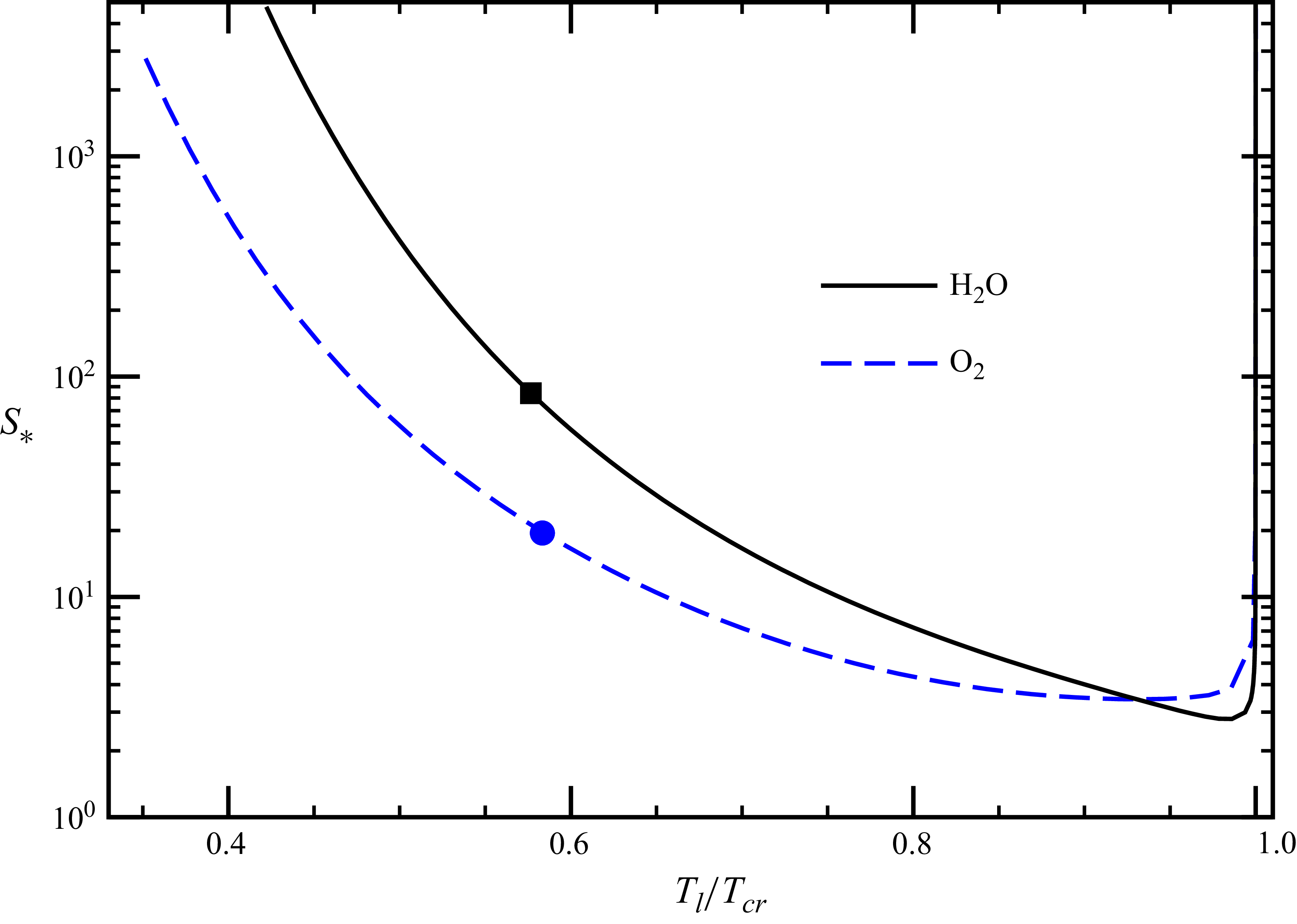
 S∗
 Tl/Tcr
 Tcr=647.13
 Tcr=154.58
 Tl/Tcr=0.575
 Tl/Tcr=0.583
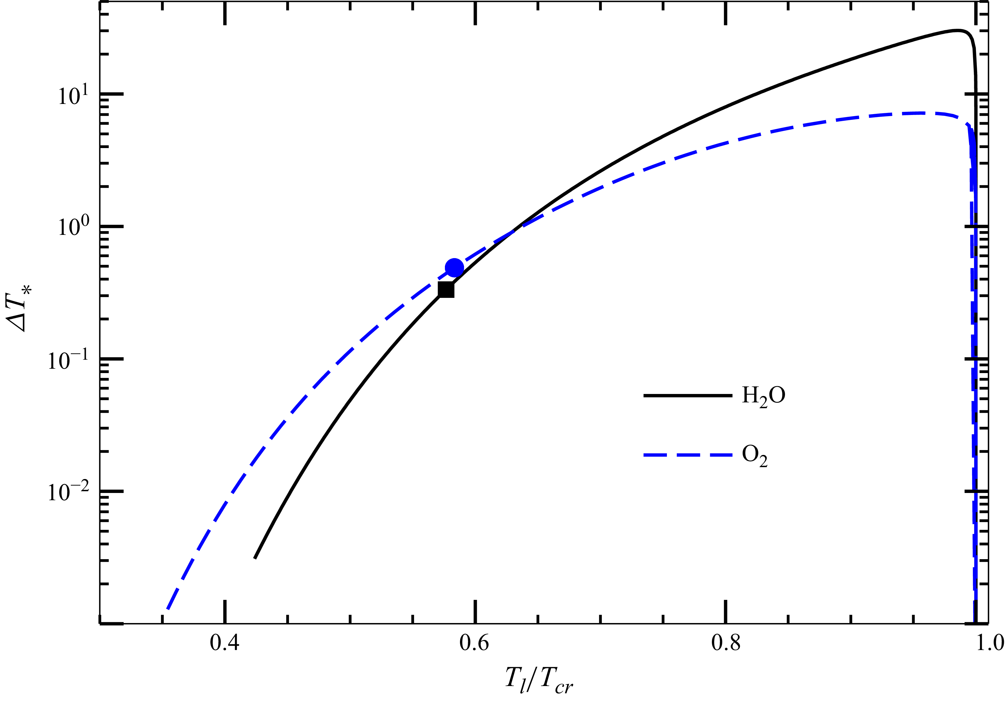
 ΔT∗
 T/Tcr
 T/Tcr=0.575
 T/Tcr=0.583
 T3p=273.16
 T/Tcr=0.422
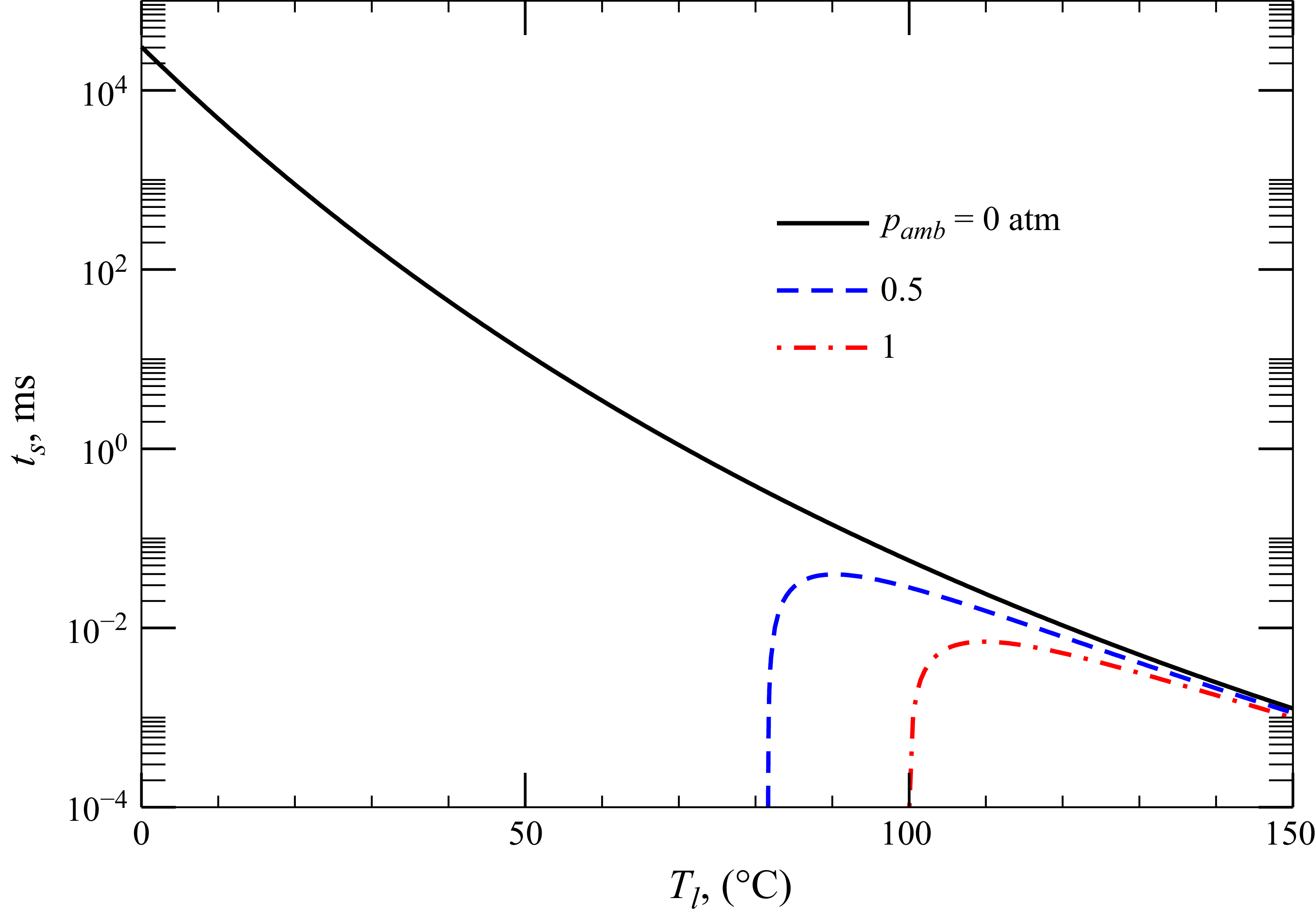
 ts
 T
 ∘
 pamb=0
 pamb=0.5
 pamb=1
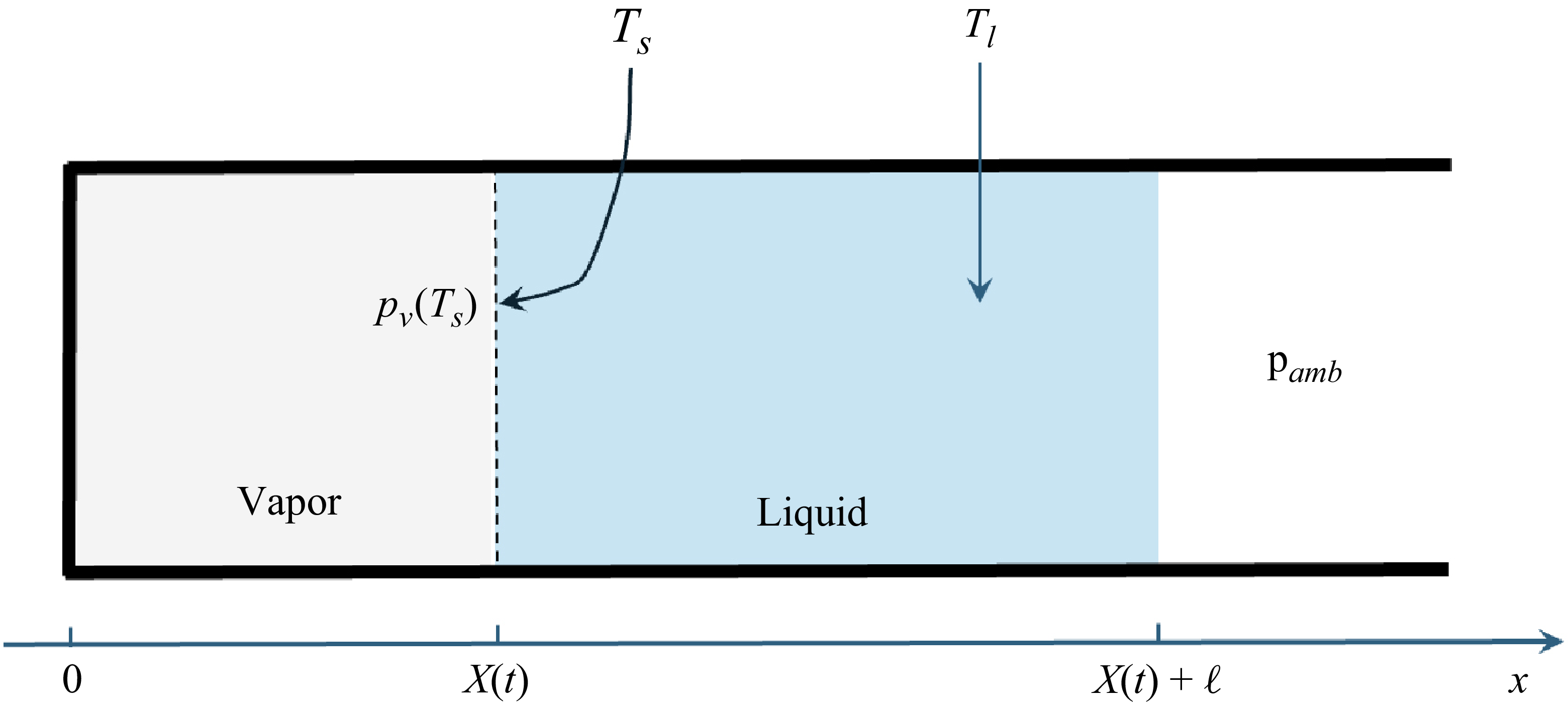
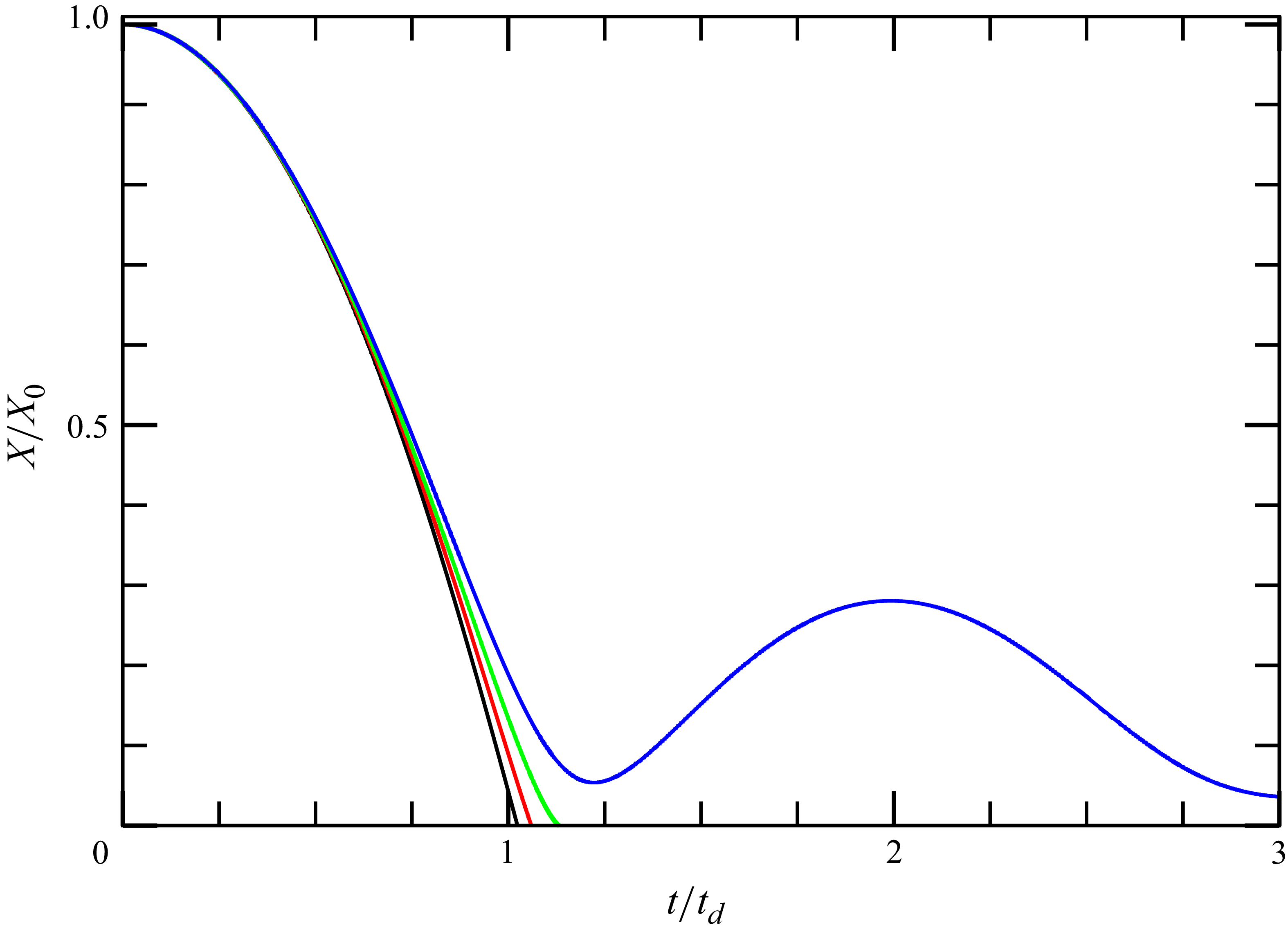
 pamb=101.3

 pamb=101.3
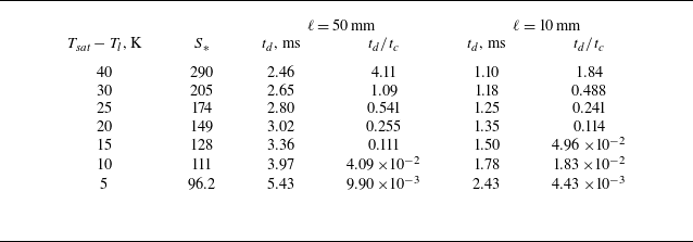
 Tsat−Tl
 S∗
 td
 td/tc
 td
 tc
 pamb=101.3
 X0=5


