2. Transverse shear flow over superhydrophobic surfaces

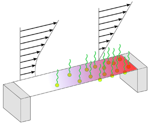
Consider the problem of steady transverse simple shear in the semi-infinite region above a periodic row of no-shear slots in an $(x,y)$ plane as shown in figure 1. The slots occupy the interval $[-b, b]$ in a period window $[-a, a]$. In the zero-Reynolds-number regime the fluid velocity ${\boldsymbol u} = (u,v)$ is governed by the Stokes equations

(2.1a,b)\begin{equation} \nabla^2 {\boldsymbol u} = \boldsymbol{\nabla} p, \quad \boldsymbol{\nabla} \boldsymbol{\cdot} {\boldsymbol u} = 0, \end{equation}

where $p$ is the fluid pressure. On the solid ridges the boundary conditions are those of no-slip:

(2.2a,b)\begin{equation} u = v = 0, \quad y=0, b \le |x| \le a. \end{equation}

In a zero-capillary-number limit based on the clean-flow surface tension the meniscus can be taken to be flat with the boundary conditions

(2.3a,b)\begin{equation} v = 0, \quad \mu \frac{\partial u}{\partial y} ={-}\frac{\partial \hat \sigma}{\partial x}, \quad y=0, 0 \le |x| \le b,\end{equation}

where $\hat \sigma (x)$ is the local surface tension value. Later we specify how this quantity depends on the local surfactant concentration, denoted by $\hat \varGamma (x)$, by specifying an equation of state. As $y \to \infty$, the flow is assumed to have the form

(2.4)\begin{equation} (u,v) \to (\dot \gamma(y + \lambda), 0),\end{equation}

where $\dot \gamma$ is the imposed far-field shear rate, and $\lambda$ is the effective slip length which will be used to characterise the degree of slip over the surface. It is usually a positive quantity which can be interpreted as the distance beneath the level $y=0$ at which the far-field slip velocity (2.4) extrapolates to zero. It measures the slip over the surface caused by the presence of the periodic menisci. For the clean flow problem the slip length is known (Philip Reference Philip1972; Crowdy Reference Crowdy2011) to be given by

(2.5)\begin{equation} \frac{a}{\rm \pi} \log \sec \left(\frac{{\rm \pi} b }{2a} \right).\end{equation}

This is discussed further in § 3.

Figure 1.

Sketch of the period window of a fluid suspended in the Cassie state over a superhydrophobic surface. The surface is composed of alternating patterns of solid surfaces, or ridges, of length $2a$, between gas-filled cavities of length $2b$. A flat meniscus, with surfactant concentration $\hat \varGamma (x)$, spans each cavity. A shear flow is applied over the surface in the direction of the grooves. The surfactant concentration leads to a Marangoni stress on the fluid. Slip is characterised by the effective slip length $\lambda$.

The primary interest of this paper is to carefully quantify the effect on the clean-flow slip length (2.5) of contamination of the menisci by insoluble surfactants having a concentration $\hat \varGamma (x)$. Let $\varGamma _0$ be the maximum packing value of this surfactant concentration. It is natural to introduce the scaled concentration $\varGamma (x)$ where $\varGamma _0 \varGamma (x) = \hat \varGamma (x)$. If $\varGamma =0$, the meniscus is clean; if $\varGamma =1$, it is maximally packed with surfactant. Non-dimensionalising lengths with respect to the half-pitch $a$ and velocities with respect to $U_0=\dot \gamma a$, the non-dimensional steady surfactant evolution equation (Halpern & Frenkel Reference Halpern and Frenkel2003) on the meniscus is

(2.6)\begin{equation} {Pe}\frac{\partial (\varGamma(x) U(x) )}{\partial x} = \frac{\partial^2 \varGamma(x) }{\partial x^2}, \quad |x| \le b,\end{equation}

where $Pe = U_0 a/D_s$ is the surface Péclet number, $D_s$ is the surface diffusion parameter and $U(x)$ is the surface slip velocity, i.e. $(u,v) = (U(x),0)$ on $y=0$. Henceforth, unless otherwise stated, all variables refer to their non-dimensional counterparts.

It will be assumed that the interfacial surfactant has adsorbed onto the menisci naturally and, consequently, that each meniscus contains the same amount of surfactant; this allows us to solve a spatially periodic problem. The total load of surfactant on each meniscus is set by imposing

(2.7)\begin{equation} \int_{{-}b}^b \varGamma(x)\, {{\rm d} x} = M,\end{equation}

where $M$ is some specified quantity. Here it is assumed that $0 \le M \le 2b$ with $M=2b$ corresponding to a meniscus maximally packed with surfactant. At the edges of the meniscus it is natural to take

(2.8)\begin{equation} \frac{\partial \varGamma }{\partial x} = 0, \quad x={\pm} b,\end{equation}

corresponding to no flux of surfactant into/out of the solid boundaries; this is reasonable because the pillars are not a source of surfactant. Equation (2.6) can be integrated immediately with respect to $x$:

(2.9)\begin{equation} {Pe}{ (\varGamma U )} = \frac{\partial \varGamma }{\partial x},\end{equation}

where a constant of integration has been set to zero. Then, because $U(\pm b)=0$, the edge conditions (2.8) will be satisfied.

To close the problem specification it is necessary to invoke an equation of state relating the surface tension $\hat \sigma (x)$ to the surfactant concentration $\hat \varGamma (x)$. In this paper we assume the nonlinear Langmuir equation of state given, in dimensional form, as

(2.10a,b)\begin{equation} \hat \sigma = \hat \sigma_0 + \hat \beta \varGamma_0 \varSigma(\hat \varGamma/\varGamma_0), \quad \varSigma(x) = \log(1-x). \end{equation}

On introducing the scalings $\hat \sigma = \mu U_0 \sigma$ for surface tension and $\hat \beta =(\mu U_0/\varGamma _0) \beta$ the equation of state becomes

(2.11a,b)\begin{equation} \sigma(x) = \sigma_0 + \beta \varSigma(\varGamma(x)), \quad \varSigma(\varGamma) = \log (1-\varGamma),\end{equation}

where we will refer to $\beta$ as the Marangoni number: it is measure of the strength of the Marangoni stresses relative to the viscous stresses associated with the imposed shear. The linearised version of the equation of state, appropriate when surfactant levels are small, is

(2.12)\begin{equation} \sigma(x) \approx \sigma_0 - \beta \varGamma(x).\end{equation}

This is sometimes referred to as the gaseous equation of state (He, Maldarelli & Dagan Reference He, Maldarelli and Dagan1991). Other equations of state (e.g. the Frumkin equation) can be used but the Langmuir equation (2.11a,b) is a good representative that affords us certain analytical and formulational advantages while still incorporating important nonlinear effects not captured by the linearised form (2.12).

The problem of characterising surface immobilisation, and the concomitant reduction in slip, for such a nonlinear equation of state is very rich. Note that on substitution of (2.11a,b) into (2.3a,b), the local Marangoni stress opposing the imposed shear flow is

(2.13)\begin{equation} \frac{\beta }{1-\varGamma} \frac{\partial \varGamma }{\partial x}.\end{equation}

If this quantity becomes large it has an adverse effect on the flow and can potentially immobilise the meniscus. The quantity (2.13) can become significant for three different reasons: if the parameter $\beta$ (the Marangoni number) is itself large, or if the surfactant gradient $\partial \varGamma /\partial x$ is large, or if $\varGamma$ is close to unity. Which one, or mixture, of these circumstances pertains is a delicate function of the surface Péclet number and total surfactant load $M$ as explored in § 8.

3. The clean-flow problem

For the clean-flow problem the solution to the mixed boundary problem just described was determined in analytical form by Philip (Reference Philip1972) using Schwarz–Christoffel theory and by Crowdy (Reference Crowdy2011) using an alternative derivation based on conformal slit mappings. It is the latter formulation that we now describe because the numerical method for the surfactant-contaminated problem described in § 7 is built on it. Crowdy (Reference Crowdy2011) has shown that the flow in the clean-flow scenario is described by the streamfunction

(3.1a–c)\begin{equation} \psi(x,y) = {\rm Im}[\bar{z}f_P(z;b)+ g_P(z;b)], \quad u = \frac{\partial \psi }{\partial y}, \quad v ={-} \frac{\partial \psi }{\partial x}, \end{equation}

where $z=x+{\rm i}y$ and

(3.2)\begin{equation} g_P(z;b) ={-} z f_P(z;b), \end{equation}

and where $f_P(z;b,a)$ is given parametrically, in terms of a conformal mapping variable $\zeta$, by

(3.3)\begin{equation} \left.\begin{array}{c@{}} z =Z(\zeta) ={-}\dfrac{{\rm i} }{\rm \pi} \log \left( -\dfrac{(\zeta-\alpha) (\zeta - 1/\alpha) }{ (\zeta-\bar{\alpha}) (\zeta - 1/\bar{\alpha}) } \right), \quad \alpha = {\rm i} \tan \left(\dfrac{{\rm \pi} b }{4} \right),\\ f_P(z;b) =F(\zeta) = \dfrac{1 }{4{\rm \pi}} \log \left( -\dfrac{(\zeta-\alpha) (\zeta - 1/\bar{\alpha}) }{ (\zeta-\bar{\alpha}) (\zeta - 1/{\alpha}) } \right).\end{array}\right\}\end{equation}

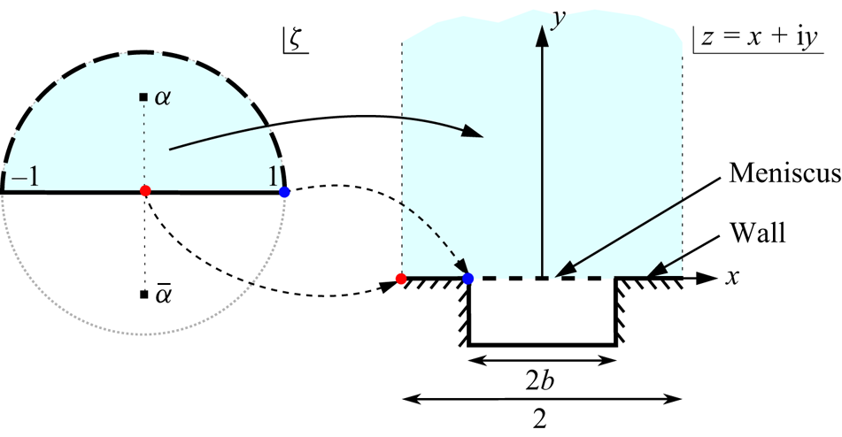
An overbar is used to denote complex conjugation. The two functions of $\zeta$ appearing as the arguments of the complex logarithms in (3.3) for $Z(\zeta )$ and $F(\zeta )$ are, respectively, a circular slit mapping and a radial slit mapping (Crowdy Reference Crowdy2011, Reference Crowdy2020b). Figure 2 shows the correspondence between points in the upper-half unit $\zeta$ disc and points in the principal period window to which it is enough to restrict consideration. The point $\zeta =\alpha$ maps to $y\to +\infty$. The real diameter $\zeta \in [-1, 1]$ is the preimage of the no-slip walls; the upper unit circle $|\zeta | =1, {\rm Im}[\zeta ] \ge 0$ is the preimage of the meniscus. The edges of the meniscus at $x=\pm b$ correspond to $\zeta = \mp 1$. As $y \to +\infty$, the flow has the form

(3.4)\begin{equation} (u,v) \to (y + \lambda_P(b), 0), \quad \lambda_P(b) = \frac{1}{\rm \pi} \log \sec \left(\frac{{\rm \pi} b}{2} \right), \end{equation}

where $\lambda _P(b)$ can be found by examining the parametric formulae (3.3) as $\zeta \to \alpha$ as shown in Crowdy (Reference Crowdy2011). It follows from (3.3) that

(3.5)\begin{equation} Z'(\zeta) = \frac{{\rm d} Z }{{\rm d} \zeta} ={-} \frac{{\rm i} }{\rm \pi} \frac{(\alpha-\bar{\alpha}) (1-|\alpha|^2)(1-\zeta^2) }{(\zeta-\alpha) (\zeta-\bar{\alpha}) (\alpha \zeta-1)(\bar{\alpha} \zeta-1)}, \end{equation}

which will be useful later. These parametric expressions (3.3) give a convenient representation of the solution. As it happens, after some algebra, $\zeta$ can be eliminated to give

(3.6a,b)\begin{equation} f_P(z;b) = \frac{{\rm i} }{2{\rm \pi}} \cos^{{-}1} \left( \frac{\cos \left(\dfrac{{\rm \pi} z }{2} \right)}{\cos \left(\dfrac{{\rm \pi} b }{2} \right)} \right), \quad U_P(x;b) ={-} 2 {\rm Re}[f_P(z;b)], \end{equation}

where $U_P(x;b)$ is the slip velocity on $y=0$. Relations (3.6a,b) are the results obtained, using very different methods, by Philip (Reference Philip1972).

Figure 2.

Schematic of the geometrical effect of the conformal mapping $z=Z(\zeta )$ given in (3.3) from the upper-half unit $\zeta$ disc to a single period of the fluid region with period $2a$ having set $a=1$. The numerical method of § 7 will be formulated in the $\zeta$ plane. The branch cut (the dotted line) between $\alpha$ and $\bar {\alpha }$ in the upper-half unit disc corresponds to the periodic sides of the fluid region (also dotted lines).

4. Slip length formulae from the reciprocal theorem

Some slip length formulae following from the reciprocal theorem for Stokes flow will be useful in what follows. The reciprocal theorem says that

(4.1)\begin{equation} \int_{\partial D} u_i \hat \sigma_{ij} n_j \, {\rm d} s = \int_{\partial D} \hat u_i \sigma_{ij} n_j \, {\rm d} s ,\end{equation}

where $\partial D$ is the boundary of the period window $D$ traversed in an anticlockwise sense, $\textrm {d} s$ is the usual arclength element whereas $\{ u_i, \sigma _{ij} \}$ and $\{ \hat u_i, \hat \sigma _{ij} \}$ are two solutions of the Stokes equations in $D$. The normal vector $n_j$ refers to the outward pointing normal. Let $\{ \hat u_i, \hat \sigma _{ij} \}$ be the velocity and stress tensor for the problem of shear flow over a superhydrophobic surface, with or without surfactants, and let $\hat \lambda$ denote the slip length associated with the flow:

(4.2)\begin{equation} \hat{\boldsymbol u} \to (y + \hat \lambda, 0), \quad {\rm as}\ y \to \infty. \end{equation}

Two useful results follow from (4.1).

The first comes on letting the comparison flow $\{ u_i, \sigma _{ij} \}$ in (4.1) be the basic Couette flow $(y,0)$. Then it follows from (4.1) that

(4.3)\begin{equation} \hat \lambda = \frac{1 }{2} \int_{{-}b}^b \hat U(x)\, {{\rm d} x}, \end{equation}

where $\hat {\boldsymbol u} = (\hat U(x),0)$ on $y=0$.

A second useful result follows on letting the comparison flow $\{ u_i, \sigma _{ij} \}$ in (4.1) be the solution (Philip Reference Philip1972; Crowdy Reference Crowdy2011) given in (3.3) or (3.6a,b) for shear flow over a periodic array of flat no-shear slots without surfactant and with slip length $\lambda _P$. In this case,

(4.4)\begin{align} \left. \int_{{-}b}^b u_i \hat \sigma_{ij} n_j \right|_{y = 0}\, {{\rm d} x} \left. -\int_{{-}1}^1 u_i \hat \sigma_{ij} n_j \right|_{y \to \infty}\, {{\rm d} x} =\left. \int_{{-}b}^b \hat u_i \sigma_{ij} n_j \right|_{y = 0}\, {{\rm d} x} \left. -\int_{{-}1}^1 \hat u_i \sigma_{ij} n_j \right|_{y \to \infty}\, {{\rm d} x}, \end{align}

where the minus signs have been added because $\textrm {d}s=-{\textrm {d} x}$ along the boundary as $y \to \infty$. Using the shear-free property of $\{ u_i, \sigma _{ij} \}$ on the interface it follows that

(4.5)\begin{equation} \left. \int_{{-}b}^b u_i \hat \sigma_{ij} n_j \right|_{y = 0}\, {{\rm d} x} = \left. \int_{{-}1}^1 u_i \hat \sigma_{ij} n_j \right|_{y \to \infty}\, {{\rm d} x} \left. -\int_{{-}1}^1 \hat u_i \sigma_{ij} n_j \right|_{y \to \infty}\, {{\rm d} x} = 2 (\lambda_P - \hat \lambda),\end{equation}

or

(4.6)\begin{equation} \hat \lambda = \left.\lambda_P - \frac{1}{2} \int_{{-}b}^b u_i \hat \sigma_{ij} n_j \right|_{y =0}\,{{\rm d} x}. \end{equation}

5. Perturbation analysis

Before proceeding, we briefly discuss scalings of the parameters to assess the value of the forthcoming perturbation analyses. Assuming some typical values for the shear rate ($\dot {\gamma }=0.1\ \mathrm {s}^{-1}$), half-period length ($a=250 \times 10^{-6}\ \mathrm {m}$), and the diffusion coefficient [$D=7\times 10^{-10}\ \mathrm {m}^2\ \mathrm {s}^{-1}$ that of sodium-decyl sulfate (SDS), an average strength surfactant, see Peaudecerf et al. (Reference Peaudecerf, Landel, Goldstein and Luzzatto-Fegiz2017)], it is found that $Pe=\dot {\gamma }a^2/D_{s}\sim O(10^2)$. This is highly dependent on the choice of length scale. For example, choosing $a=2\times 10^{-3}\ \mathrm {m}$ means $Pe\sim O(10^3)$. But smaller length scales and shear rates can lead to Péclet numbers of $O(1)$ or smaller. The choice of $a=100 \times 10^{-6}\ \mathrm {m}$ with a shear rate of $\dot {\gamma }=0.01\ \mathrm {s}^{-1}$ means $Pe\sim O(10^0)$, a value small enough such that a small $Pe$ expansion is useful. Some typical values of the Marangoni number ($\beta =\hat {\beta }\varGamma _0/(a\mu \dot {\gamma })$) can also the generated. The dimensional constant $\hat {\beta }=RT$, where $R$ is the universal gas constant and $T$ the liquid temperature in degrees Kelvin, such that $\hat {\beta }\sim O(10^2)$. The maximum packing value is $\varGamma _0=3.9 \times 10^{-6}\ \mathrm {{mol}}\ \mathrm {m}^{-2}$ for SDS. Assuming $\mu$ to be the viscosity of water and using the same three parameter sets used to evaluate $Pe$ above, $\beta \sim O(10^6)$ in the case that $Pe\sim O(10^2)$, $\beta \sim O(10^5)$ for $Pe\sim O(10^3)$ and $\beta \sim O(10^7)$ when $Pe\sim O(10^0)$. This scaling indicates that the value of the perturbation analysis for small $\beta$ may only be in the validating the numerical results; however, the small $Pe$ limit may be a useful result for cases in which the length scales are small.

With these scalings in mind we consider a regular perturbation analysis in two cases: $Pe \ll 1$ and $\beta \ll 1$. This is done to gain insight into the physical mechanisms, particularly the small $Pe$ analysis, and to help evaluate the validity of the later numerical solutions. In each case, considered separately in the next two subsections, having assumed a regular perturbation expansion in each parameter, the validity of that expansion will require restrictions on the other parameters in the problem.

5.1. Perturbation analysis for small $Pe$

First suppose that $Pe \ll 1$ and assume a regular perturbation expansion:

(5.1a–c)\begin{equation} \varGamma = \varGamma_0 + Pe \varGamma_1 + \cdots, \quad U = U_0 + Pe U_1 + \cdots, \quad \lambda = \lambda_0 + Pe \lambda_1 + \cdots.\end{equation}

The circumstances under which such a regular expansion is expected to hold will emerge from the analysis. Substitution into (2.9) leads to

(5.2)\begin{equation} {Pe} (\varGamma_0 + Pe \varGamma_1 + \cdots ) (U_0 + Pe U_1 + \cdots ) = \frac{\partial }{\partial x}(\varGamma_0 + Pe \varGamma_1 + \cdots ). \end{equation}

The equation arising at ${O}(Pe^0)$ is

(5.3)\begin{equation} 0 = \frac{\partial \varGamma_0 }{\partial x}, \end{equation}

implying that

(5.4)\begin{equation} \varGamma_0 = \frac{M }{2b},\end{equation}

this constant chosen to satisfy (2.7). Therefore, in the zero surface Péclet limit the surfactant concentration is not affected by the ambient flow and pure diffusion leads to a uniform surfactant concentration. This leading-order solution satisfies the edge conditions (2.8). As the associated Marangoni stress is zero the leading-order slip velocity $U_0$ must be the surface slip velocity in Philip's solution (Philip Reference Philip1972; Crowdy Reference Crowdy2011) with $\lambda _0$ the associated slip length:

(5.5a,b)\begin{equation} U_0 = U_P(x;b), \quad \lambda_0 = \lambda_P(b).\end{equation}

At ${O}(Pe)$ we find from (5.2) that

(5.6)\begin{equation} \frac{\partial \varGamma_1 }{\partial x} = \varGamma_0 U_0.\end{equation}

The edge conditions (2.8) require that $\partial \varGamma _1/\partial x =0$ at $\pm b$ which are satisfied because $U_0=U_P(x;b)$ which vanishes at the edges $\pm b$ of the no-shear slot. From (5.4), (5.5a,b) and (5.6) it follows that

(5.7)\begin{equation} \varGamma_1(x) = \varGamma_0 \left [ \int_{{-}b}^x U_0(x) \, {{\rm d} x} + A \right ], \end{equation}

where $A$ is a constant determined by enforcing (2.7), namely,

(5.8)\begin{equation} \int_{{-}b}^b \varGamma_1(x)\, {{\rm d} x} = 0 \ {\rm or} \int_{{-}b}^b \left[ \int_{{-}b}^x U_0(x')\, {{\rm d} x}' \right] {{\rm d} x} + 2b A= 0.\end{equation}

Using $\hat \sigma _{ij}$ to denote the stress tensor associated with the flow the stress condition on the interface can be written

(5.9)\begin{equation} \hat \sigma_{ij} n_j = \beta \varSigma'(\varGamma) \frac{\partial \varGamma(x) }{\partial x} t_i,\end{equation}

where $t_i$ denotes components of the unit tangent, and where now $n_j$ refers to the fluid-inward pointing normal. Now provided the quantity

(5.10)\begin{equation} \frac{\beta }{1-\varGamma_0},\end{equation}

is of order unity, then, on substitution of (5.1a–c) into (5.9), it follows that

(5.11)\begin{equation} \hat \sigma_{ij} n_j ={-}\frac{\beta Pe }{1- \varGamma_0} \frac{\partial \varGamma_1(x) }{\partial x} t_i + {{O}}(Pe^2). \end{equation}

With (5.5a,b) and (5.6), formula (4.6) gives

(5.12)\begin{equation} \lambda = \lambda_P(b) -\frac{Pe \beta \varGamma_0 }{2 (1-\varGamma_0)} \int_{{-}b}^b U_P(x;b)^2 \,{{\rm d} x} + {{O}}(Pe^2). \end{equation}

This is expected to give a good approximation formula for the effective slip length at small $Pe$ provided the quantity (5.10) is of order unity. It is therefore not expected to be accurate (even if $Pe$ is small) when $\beta$ is large or for values of $M$ close to its maximum value $2b$ (for which, according to (5.4), $\varGamma _0$ is close to unity).

5.2. Perturbation analysis for small $\beta$

Suppose instead that $\beta \ll 1$ and assume a different regular perturbation expansion

(5.13a–c)\begin{equation} \varGamma = \tilde \varGamma_0 +\beta \tilde\varGamma_1 + \cdots, \quad U = \tilde U_0 + \beta \tilde U_1 + \cdots, \quad \lambda = \tilde \lambda_0 + \beta \tilde \lambda_1 + \cdots. \end{equation}

On substitution into (2.9), the surfactant evolution equation can be expanded as

(5.14)\begin{equation} {Pe}(\tilde \varGamma_0 + \beta \tilde\varGamma_1 + \cdots) (\tilde U_0 + \beta \tilde U_1 + \cdots) =\frac{\partial }{\partial x} (\tilde \varGamma_0 + \beta \tilde \varGamma_1 + \cdots). \end{equation}

At ${O}(\beta ^0)$ the equation is

(5.15)\begin{equation} Pe(\tilde \varGamma_0 \tilde U_0)=\frac{\partial \tilde \varGamma_0 }{\partial x}.\end{equation}

The stress condition becomes

(5.16)\begin{align} \left(\frac{\partial \tilde U_0 }{\partial y} + \beta \frac{\partial \tilde U_1 }{\partial y} \right) &= \frac{\beta }{1- ( \tilde \varGamma_0+ \beta \tilde \varGamma_1 + {\cdots})} \left(\frac{\partial \tilde \varGamma_0 }{\partial x} + \beta \frac{\partial \tilde \varGamma_1 }{\partial x} + \cdots \right)\nonumber\\ &=\beta \left(\frac{1 }{1- \tilde \varGamma_0 } + \frac{\beta \tilde \varGamma_1 }{(1- \tilde \varGamma_0)^2} + \cdots \right) \left(\frac{\partial \tilde \varGamma_0 }{\partial x} + \beta \frac{\partial \tilde \varGamma_1 }{\partial x} + \cdots \right). \end{align}

Provided the quantity

(5.17)\begin{equation} \frac{1 }{1- \tilde \varGamma_0 }\frac{\partial \tilde \varGamma_0}{\partial x},\end{equation}

is of order unity, then, at ${O}(\beta ^0)$, (5.16) gives

(5.18)\begin{equation} \frac{\partial \tilde U_0 }{\partial y} = 0, \end{equation}

which is a zero-shear-stress condition. As the slip velocity must vanish on the no-slip ridges, then, as in § 5.1, we infer once again that the leading-order velocity field is given by Philip's solution so that

(5.19a,b)\begin{equation} \tilde U_0(x) = U_P(x;b), \quad \tilde \lambda_0 = \lambda_P(b).\end{equation}

The distribution $\tilde \varGamma _0(x)$ can now be found by solving (5.15) and using (5.19a,b):

(5.20)\begin{equation} \tilde \varGamma_0(x) = \tilde A \exp \left({-}Pe\int_{x}^{b}U_P(x';b)\mathrm{d} x'\right),\end{equation}

where the constant $\tilde A$ is determined by enforcing (2.7), i.e.

(5.21)\begin{equation} \int_{{-}b}^{b} \tilde \varGamma_0(x)\, {{\rm d} x} =M. \end{equation}

With the same assumption imposed earlier on (5.17), at ${O}(\beta )$, the stress condition (5.16) gives

(5.22)\begin{equation} \frac{\partial \tilde U_1 }{\partial y} = \frac{1 }{1-\tilde \varGamma_0} \frac{\partial \tilde \varGamma_0 }{\partial x},\end{equation}

where, given (5.20), the right-hand side is now known implying that the first-order Marangoni stress on the interface is also known. Use of (5.19a,b), (5.20) and (5.22) in (4.6) gives the slip length as

(5.23)\begin{align} {\lambda} = \lambda_P(b) -\frac{\beta Pe }{2} \int_{{-}b}^{b}U_P(x;b)^2 \left(\frac{ \tilde A \exp \left({-}Pe \displaystyle \int_{x}^{b}U_P(x';b)\, \mathrm{d} x' \right) }{ 1- \tilde A \exp \left({-}Pe\displaystyle \int_{x}^{b}U_P(x';b)\,\mathrm{d} x' \right) }\right) \,\mathrm{d} x + {{O}}(\beta^2).\end{align}

This is expected to be a good approximation for small $\beta$ provided the quantity (5.17), or equivalently from (5.15), the quantity

(5.24)\begin{equation} \frac{Pe \tilde \varGamma_0~\tilde U_0 }{1- \tilde \varGamma_0 },\end{equation}

is of order unity. Formula (5.23) can therefore be expected to lose accuracy as $Pe$ becomes large, or if $\tilde \varGamma _0(x)$ gets close to unity at any point on the meniscus. In such circumstances, the regular perturbation analysis just performed is not expected to be valid. In fact, we can say more as $Pe \to \infty$. In that limit the quantity (5.24) is much larger than unity and we expect the leading-order slip profile $U_0$ to be quite different from Philip's slip velocity as given in (5.19a,b): indeed, we expect the slip velocity and slip length at zero Marangoni number to be given by

(5.25a–c)\begin{equation} U_P(x;\hat b), \quad {\rm and} \quad \lambda_P(\hat b), \quad 2 \hat b = 2b - M. \end{equation}

This is because at infinite surface Péclet number and at zero Marangoni number all surfactant will be advected to the downstream edge of the meniscus with no countervailing Marangoni stress to modify the surfactant concentration, which must satisfy (2.7), from having a jump discontinuity (akin to that of a Heaviside function) as follows:

(5.26)\begin{equation} \varGamma(x) = \left \{ \begin{array}{@{}ll} 0, & -b \le x < b-M, \\ 1, & b-M < x \le b. \end{array} \right .\end{equation}

As $0 \le M \le 2b$, the two limiting cases are a clean meniscus as $M \to 0$ and a fully loaded meniscus as $M \to 2b$. These theoretical expectations are borne out by the numerical calculations in § 8.

6. Complex variable formulation

In this section we describe the complex variable approach used by Crowdy (Reference Crowdy2011) which will provide the basis for a numerical approach to the problem involving insoluble surfactants to be described in § 7; it affords various advantages to be discussed there. Using the non-dimensionalisation introduced earlier, any incompressible Stokes flow in a two-dimensional $(x,y)$ plane is described biharmonic streamfunction $\psi (z,\bar {z})$ given by

(6.1a–c)\begin{equation} \psi(z, \bar{z}) = {\rm Im}[\bar{z}f(z) + g(z)], \quad (u,v) = \left( \frac{\partial \psi }{\partial y}, -\frac{\partial \psi }{\partial x} \right), \quad u - {\rm i} v = 2 {\rm i} \frac{\partial \psi }{\partial z}, \end{equation}

where $f(z)$ and $g(z)$ are two functions of $z =x + \textrm {i} y$. From the Stokes equations it can be shown that the fluid pressure $p$, the vorticity $\omega = -\nabla ^2 \psi = -4 \partial ^2 \psi /\partial z \partial \bar {z}$ and the fluid rate-of-strain tensor $e_{ij}=(1/2)(\partial u_i/\partial x_j + \partial u_j/\partial x_i)$ are related to $f(z)$ and $g(z)$ through

(6.2a–c)\begin{align} 4 f'(z) = {p} - {\rm i} \omega, \quad u - {\rm i} v ={-} \overline{f(z)} + \bar{z} {f'(z)} + {g'(z)} , \quad e_{11} + {\rm i} e_{12} = z \overline{f''(z)} + \overline{g''(z)}, \end{align}

where primes denote differentiation with respect to the argument of the function. A derivation of these fundamental relations is given in an appendix of Crowdy (Reference Crowdy2020a). The complex form of the fluid stress on the boundary, i.e. $\sigma _{ij} = -p n_i+ 2 e_{ij} n_j$, is

(6.3a,b)\begin{equation} - 2 {\rm i}\frac{{\rm d} H }{{\rm d} x}, \quad H(z,\bar{z}) \equiv f(z) + z \overline{f'(z)} + \overline{g'(z)}.\end{equation}

For a far-field simple shear flow with $(u,v) \sim (y+\lambda, 0)$ as $|z| \to \infty$ we need

(6.4a,b)\begin{equation} f(z) \sim \frac{{\rm i} }{4} z + {{O}}(1), \quad g(z) \sim{-} \frac{{\rm i} }{4} z^2 + {{O}}(z).\end{equation}

The choice

(6.5)\begin{equation} g(z) ={-}z f(z), \end{equation}

is consistent with the far-field shear conditions (6.4a,b) and ensures that $y=0$ is a streamline. This means

(6.6)\begin{equation} g'(z) ={-}z f'(z) -f (z).\end{equation}

It follows from (6.6) that the complex velocity field is

(6.7)\begin{equation} u - {\rm i} v ={-}\bar{f} + \bar{z} f'(z) + g'(z) ={-}\overline{f(z)} + \bar{z} f'(z) -z f'(z) -f(z). \end{equation}

On $y=0$, where $\bar {z}=z$, this simplifies to

(6.8)\begin{equation} u - {\rm i} v ={-}2 {\rm Re}[f(z)] := U(x),\end{equation}

where we introduce $U(x)$ to denote the slip velocity at $y=0$. The fluid stress on the flat interface must balance the Marangoni stress:

(6.9)\begin{equation} \sigma_{ij} n_j ={-}\frac{{\rm d} \sigma(x) }{{\rm d} x} t_i. \end{equation}

From (6.6) it follows that, on $y=0$,

(6.10)\begin{equation} H = f(z) + z \overline{f'(z)} - \overline{z f'(z) + f (z)} = f(z) - \overline{f(z)} = 2 {\rm i}\,{\rm Im}[f(z)], \end{equation}

and, from (6.3a,b),

(6.11)\begin{equation} - 2 {\rm i} \frac{{\rm d} H }{{\rm d} x} = 4 \frac{{\rm d}\, {\rm Im}[f(x)] }{{\rm d} x} ={-}\frac{{\rm d} \sigma(x) }{{\rm d} x} ={-}\beta \varSigma'(\varGamma) \frac{{\rm d} \varGamma }{{\rm d} x}. \end{equation}

Integrating this along the meniscus from the upstream edge at $x=-b$ gives

(6.12)\begin{equation} {\rm Im}[f(x)] ={-} \frac{\beta}{4} {[\varSigma(\varGamma(x)) - \varSigma(\varGamma({-}b))]}:=\frac{\chi(x) }{2},\end{equation}

where we have introduced the new function $\chi (x)$. This integration along the interface is itself significant: it means that, in the numerical method to be described in § 7, the interfacial Marangoni stresses are never actually computed and $f(x)$ depends solely of the absolute difference in dimensionless surface tension between $x$ and the upstream edge $-b$.

It follows from (6.8) and (6.12) that, on $y=0$,

(6.13)\begin{equation} f(x) ={-} \frac{U(x) }{2} + \frac{{\rm i} \chi(x) }{2}.\end{equation}

Now introduce the modified analytic function

(6.14)\begin{equation} q(z) ={-} 2 {\rm i} f(z) - \frac{z }{2}, \end{equation}

which, from (6.4a,b), is seen to be an analytic function of $z$ in the period window including as $y \to +\infty$. On $y=0$ it follows from (6.13) that

(6.15)\begin{equation} q(x) = \chi(x) - \frac{x }{2} + {\rm i} U(x).\end{equation}

This means that the function $q(z)$ composed with the mapping function, namely,

(6.16)\begin{equation} Q(\zeta) \equiv q(Z(\zeta)), \end{equation}

where $Z(\zeta )$ is given in (3.3), is analytic in the upper-half unit disc including at $\zeta =\alpha$, the preimage of the point at infinity $y \to \infty$.

An important observation from (6.15) is that, on the no-slip wall, corresponding to the real diameter $\bar {\zeta } = \zeta$,

(6.17)\begin{equation} 0 = U(x) = {\rm Im}[q(z)] = {\rm Im}[Q(\zeta)]. \end{equation}

This implies that

(6.18)\begin{equation} Q(\zeta) - \overline{Q(\zeta)} = 0, \ {\rm or}\ \bar{Q}(\zeta) = Q(\zeta), \end{equation}

where $\bar {Q}(\zeta )\equiv \overline {Q(\overline {\zeta })}$ is the Schwarz conjugate to $Q(\zeta )$. As $Q(\zeta )$ is analytic in the upper-half unit disc and satisfies (6.18) it follows from the Schwarz reflection principle that $Q(\zeta )$ is analytic everywhere in the unit $\zeta$ disc.

It can now be shown (details are given in Appendix A) that $Q(\zeta )$ can be given explicitly on use of the classical Poisson integral formula for the unit disc:

(6.19)\begin{equation} Q(\zeta) = \frac{1 }{2 {\rm \pi}{\rm i}} \oint_{|\zeta'|=1} \frac{{\rm d} \zeta' }{\zeta'} \frac{\zeta' + \zeta }{\zeta'-\zeta} \left( \chi(Z(\zeta')) - \frac{Z(\zeta') }{2} \right).\end{equation}

This formula is important for the numerical method described in § 7: it provides the boundary slip velocity (the imaginary part of $Q(\zeta )$) associated with any given Marangoni stress distribution on the meniscus (which furnishes the real part of $Q(\zeta )$). We note that up to this point in the complex variable formulation no assumptions about $\varGamma$ have been made. As a consequence (6.19) is valid for any similar problem in which an equation of state for surface tension can be written down.

7. Numerical method based on the conformal mapping formulation

We now describe the numerical scheme. A key step is to pose the Laurent series representation in $\zeta$ given by

(7.1)\begin{equation} \log \left( \frac{1- \varGamma(x) }{\varGamma(x) } \right) = b_0 + \sum_{n=1}^\infty \left( b_n \zeta^n + \frac{{b_{n}} }{\zeta^n} \right), \end{equation}

where $\{ b_n \in \mathbb {R} \}$ is a set of real coefficients to be determined, after suitable truncation, by the numerical algorithm. The representation (7.1) may appear curious at first but several features of it should be pointed out because it builds in important requisite properties of the solution. It is worth remarking that several other choices of ansatz were tried before this one, but they all were significantly less robust leading to schemes that failed to converge at much smaller Péclet numbers.

First, as discussed by Crowdy (Reference Crowdy2011, Reference Crowdy2013), use of the conformal mapping variable $\zeta$ intrinsically captures the expected square root singularity, as a function of the physical variable $z$, at the meniscus edges $\pm b$. Written as a function of $\zeta$, however, those singularities do not appear in any explicit way (they have been ‘uniformised’) and afford a simpler-to-handle Laurent series representation (7.1). This offers both theoretical advantages (Crowdy Reference Crowdy2011, Reference Crowdy2021) but also significant numerical ones too, as will become evident as the simplicity and effectiveness of the following scheme emerges.

Second, the representation (7.1) automatically builds in the physical requirement

(7.2)\begin{equation} 0 \le \varGamma(x) \le 1.\end{equation}

If (7.2) fails to be true, it is clear that (7.1) with real coefficients $\{ b_n\}$ will not be a consistent representation.

For a given value of $b$ the mapping function (3.3) is known. The first step is to truncate (7.1) at some integer $N$. A continuation procedure from small values of $Pe$ is then initialised by choosing

(7.3)\begin{equation} b_0 = \log \left(\frac{1-\varGamma_0 }{\varGamma_0} \right), \quad \varGamma_0 = \frac{M }{2b}, \quad b_n = 0,\ n = 1, \ldots, N, \end{equation}

where $M$ has been specified. This choice is prompted by the uniform coverage expected at $Pe=0$ from the perturbation analysis of § 5.1. An analogous continuation procedure can also be carried out as the Marangoni number $\beta$ is increased from zero using the perturbation analysis of § 5.2 as the initial guess. It follows by straightforward algebraic manipulation of (7.1) that

(7.4)\begin{align} \left.\begin{array}{c@{}} \displaystyle \log \varGamma(x) ={-} \log \left(1+ \exp{ \left [b_0 + \sum_{n=1}^N \left( b_n \zeta^n + \dfrac{{b_{n}} }{\zeta^n} \right)\right ]} \right), \\ \displaystyle \varGamma(x) = \left(1+ \exp{ \left [b_0 + \sum_{n=1}^N \left( b_n \zeta^n + \dfrac{{b_{n}} }{\zeta^n} \right)\right ]} \right)^{{-}1},\\ \displaystyle \log (1-\varGamma(x)) =b_0 + \sum_{n=1}^N \left( b_n \zeta^n + \dfrac{{b_{n}} }{\zeta^n} \right) - \log \left(1+ \exp{ \left [b_0 + \sum_{n=1}^N \left( b_n \zeta^n + \dfrac{{b_{n}} }{\zeta^n} \right)\right ]} \right), \end{array}\right\} \end{align}

all of which are needed in what follows. The function $\chi (x)$ can be found from its definition (6.12) and the equation of state (2.11a,b):

(7.5)\begin{equation} \chi(x) = {-\frac{\beta}{2}}\log \left( \displaystyle\frac{1- \varGamma(x) }{1-\varGamma({-}b)}\right), \end{equation}

which, up to an unimportant constant, is given in terms of the coefficients $\{ b_n \in \mathbb {R} \}$ by the final formula in (7.4). As $Z(\zeta )$ is given in (3.3), formula (6.19) can now be used to determine the surface slip $U(x)$, as well as the integral

(7.6)\begin{equation} \int_x^b U(x')\, {{\rm d} x}'.\end{equation}

In practice, use of the Poisson integral formula can be circumvented by use of series expansions and fast Fourier transforms. The reason for computing (7.6) is that, on use of an integrating factor in the surfactant evolution equation (2.9), we can write

(7.7)\begin{equation} {\log \varGamma(x) }= \log A_0 - {Pe \int_x^b U(x')\, {{\rm d} x}' }, \end{equation}

for some constant $A_0$. Note that, in a step found to be important for robust convergence of the numerical iteration, the integration in (7.7) is taken over an interval that includes the downstream portion of the meniscus that is expected to be contaminated with surfactant in most circumstances.

An important observation is that we now have two expressions for $\log \varGamma (x)$: one is given by the first formula in (7.4), another by (7.7). These are supposed to be consistent when evaluated at the solution. The numerical method is then as follows. Given an initial guess of coefficients $\{ b_n | n=0,1, \ldots, N \}$, (7.5) is used with (6.19) to determine the surface slip $U(x)$, which is the imaginary part of $Q(\zeta )$, as a Laurent series in $\zeta$. Now (7.6) can be evaluated numerically. This integral is then fed into (7.7) to evaluate $\log \varGamma (x)$. The Laurent series of $\log \varGamma (x)$, valid on $|\zeta |=1$, as given both by (7.7) and by the first formula in (7.4) are then determined. The required Laurent series coefficients can be readily computed using fast Fourier transforms. A set of $N$ equations to update the initial guess for the truncated set of coefficients $\{ b_n | n=0,1, \ldots, N \}$ follows by equating powers of $\zeta ^n$ for $n=1, \ldots, N$ in these two Laurent series with an additional equation furnished by the mass constraint

(7.8)\begin{equation} \int_{{-}b}^b \varGamma(x)\, {{\rm d} x} = M,\end{equation}

where $\varGamma (x)$ is calculated using the second formula in (7.4). The resulting set of $N+1$ equations for the $N+1$ real coefficients $\{ b_n | n=0,1, \ldots, N \}$ can then be solved. The solutions to follow in § 8 are computed using at most 150 Laurent coefficients, with the majority of the calculations requiring significantly fewer. Usually a quasi-Newton is found to be sufficient to solve for the coefficients but Newton method's is sometimes necessary to ensure convergence when the surfactant load is large.

For small $Pe \ll 1$ a check on the numerical method is to verify that the computed $\varGamma (x)$ agrees, to first order in $Pe$, with that obtained by the perturbation theory in § 5.1. Similar checks are afforded by the perturbation theory for small $\beta$ given in § 5.2.

When $Pe \to \infty$ we expect a stagnant cap of length $2b-2l$ to form adjacent to the downstream edge at $x=b$ where the parameter $l$ can be determined by using Philip's solution (3.6a,b) and enforcing the condition (7.8). With respect to a shifted frame of reference where the clean portion of the interface now occupies the interval $[-l,l]$ we have

(7.9)\begin{equation} \chi(x) = 2\,{\rm Im}[f_P(z;l)],\end{equation}

where $f_P$ is defined in (3.6a,b) and the contaminated portion of the interface corresponds to the interval $[l, 2b-l]$. For the Langmuir equation of state (2.11a,b) we have

(7.10)\begin{equation} \varGamma(x) = 1- {\rm e}^{{-}2 \chi(x)/\beta}, \end{equation}

so (7.8), which is a single nonlinear equation for $l$, is

(7.11)\begin{equation} \int_{l}^{2b-l} (1- {\rm e}^{{-}4\,{\rm Im}[f_P(z;l)]/\beta})\, {{\rm d} x} = M. \end{equation}

Once $l$ is determined from this condition the associated slip length will be

(7.12)\begin{equation} \lambda = \lambda_P(l).\end{equation}

Details of such a procedure assuming a linear equation of state have been worked out by Baier & Hardt (Reference Baier and Hardt2021). A completely analogous determination of the edges of two stagnant caps was used by Siegel (Reference Siegel1999) for a two-dimensional bubble in an extensional flow, and by Sadhal & Johnson (Reference Sadhal and Johnson1983) in a three-dimensional bubble problem.

8. Characterisation of the numerical solutions

The important dimensionless parameters are the surface Péclet number, $Pe$, the Marangoni number, $\beta$, the total amount of surfactant on each meniscus $M$, and the interface fraction $b$. A useful parameter in what follows is

(8.1)\begin{equation} \bar{\varGamma}=\frac{M }{2b}, \end{equation}

which represents the average surfactant concentration on the interface.

8.1. Effect of $Pe$

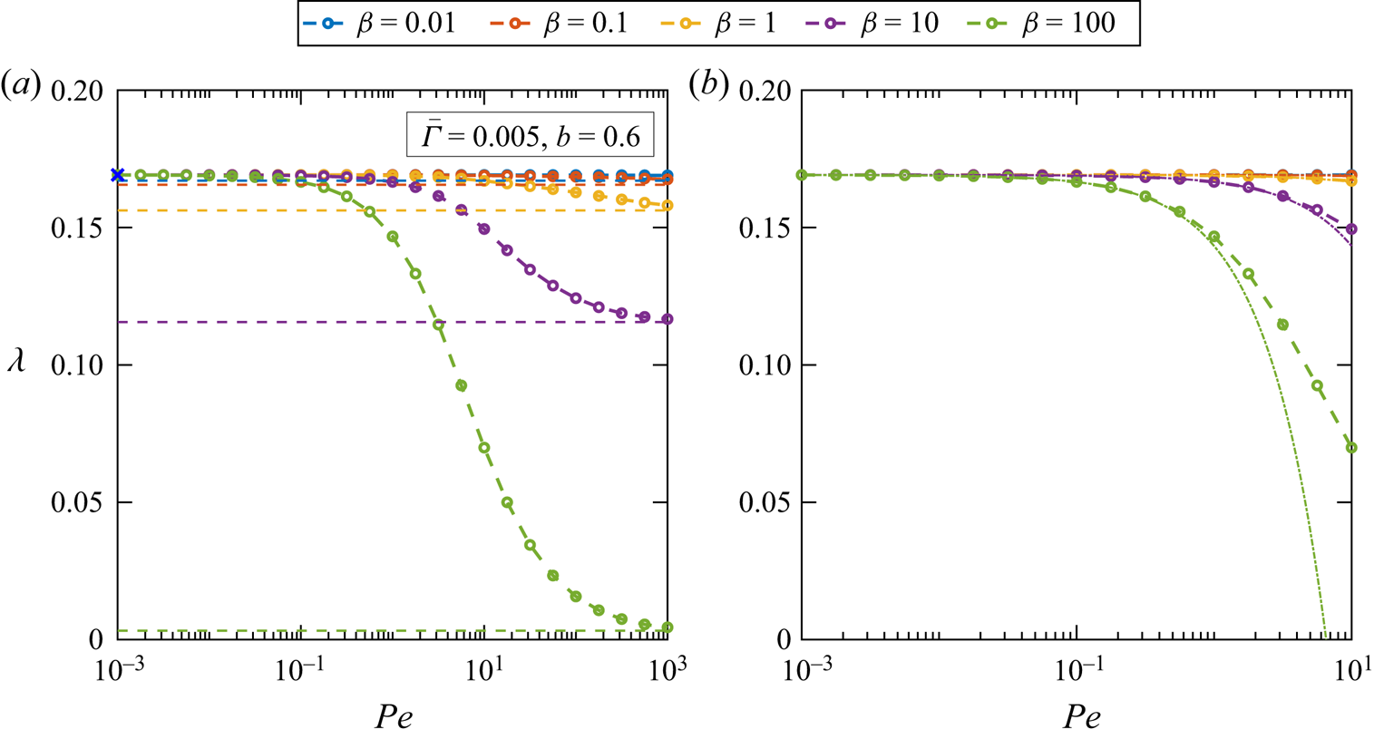
To investigate the effect of $Pe$ on the effective slip lengths, solutions have been calculated for a large range of $Pe$ spanning several decades and for several different values of $b$, $\bar {\varGamma }$ and $\beta$. Figure 3(a) shows the slip length over a range of $Pe$ and for five values of $\beta$ with $\bar {\varGamma } = 0.005$ and $b=0.6$. As $Pe\rightarrow 0$ the slip lengths converge to that of a shear-free meniscus as indicated by the dotted lines in the refined view shown in figure 3(b) and corroborating expectations from the perturbation theory of § 5.1. This is because the diffusive flux becomes dominant, yielding a uniform surfactant distribution with no Marangoni stresses. Agreement with the perturbation analysis is good here because, for this choice of parameters, the quantity in (5.10) is of order unity. For this quite small surfactant level $\bar {\varGamma }$ the dashed lines confirm that the solutions converge to give the slip length associated with the $Pe\rightarrow \infty$ limit (7.12) discussed at the end of § 7.

Figure 3.

(a) Slip length as a function of $Pe$ for different values of $\beta$. The horizontal dashed lines show the limit for $Pe\rightarrow \infty$ as given by (7.12). (b) Refined view of the slip length curves for small $Pe$. The dotted lines are from the small $Pe$ analysis and are given by (5.12). In both (a) and (b) $\bar {\varGamma } = 0.005$ and $b=0.6$.

Figures 3(a) and 3(b) also show that, for small $\beta$, and for this small value of $\bar {\varGamma } = 0.005$, the slip length is hardly affected by the presence of the surfactant, irrespective of the value of $Pe$. As $\bar {\varGamma }$ is small the Langmuir equation of state behaves linearly, i.e. like (2.12), so that when $\beta$ is small very little shear stress is caused by the surfactant build-up. This means the stagnant cap as $Pe\rightarrow \infty$ is expected to be very small. However, we note, as discussed in § 5, that small values of $\beta$ are not physically representative for these systems so this would be a phenomenon rarely seen in practice. This also explains the limited effect of increasing $Pe$ at small values of $\beta$. As $\beta$ increases, however, the shear stresses generated are enough to retard or even nearly immobilise the meniscus at high $Pe$. This causes the dramatic decreases in slip length for larger values of $\beta$ evident in figure 3(a).

Figures 4(a) and 4(b) show velocity and surfactant concentration profiles at different Péclet numbers when $\beta = 0.01$ for this value of $\bar {\varGamma } = 0.005$. Although the surfactant concentrations in figure 4(b) have large gradients at high $Pe$, because $\beta$ is small these concentrations have very little effect on the slip velocities in 4(a). This also explains the limited effect of increasing $Pe$ on the slip lengths in figure 3(a) for this value of $\beta$. For a larger value of $\beta$, figures 5(a) and 5(b) show velocity and concentration profiles for different Péclet numbers when $\beta = 10$. Now $\beta$ is sufficiently large that the surfactant build up at higher $Pe$ retards the flow: there are now noticeably reduced slip velocities at the downstream edge of the meniscus in figure 5(a). As $Pe\rightarrow \infty$, the section of the domain contaminated with surfactant is immobilised whereas the rest is shear free; this is the expected ‘stagnant-cap’ regime discussed in § 7. The stagnant cap is even more noticeable in figures 6(a) and 6(b) which show velocity and concentration profiles for a range of Péclet numbers for the even higher value $\beta = 100$. In this case, $\beta$ is so large that the meniscus is almost entirely immobilised as $Pe$ grows, with only a small section of the meniscus exhibiting any slip by the time $Pe=1000$. Moreover, in this case, the surfactant concentration tends to a linear profile with slope $(1-\bar {\varGamma })/\beta$. This happens because the shear stress of a completely immobilised meniscus must equal the far-field shear rate which has been set to unity.

Figure 4.

(a) Slip velocity profiles and (b) surfactant concentrations for different $Pe$ with $\bar {\varGamma }$ = 0.005, $b=0.6$ and $\beta =0.01$.

Figure 5.

(a) Slip velocity profiles and (b) surfactant concentrations for different $Pe$ with $\bar {\varGamma }$ = 0.005, $b=0.6$ and $\beta =10$.

Figure 6.

(a) Slip velocity profiles and (b) surfactant concentrations for different $Pe$ with $\bar {\varGamma } = 0.005$, $b=0.6$ and $\beta =100$.

If $\bar {\varGamma }$ is sufficiently large, and/or $\beta$ is sufficiently small, accumulating surfactant can reach levels close to one and the nonlinearity in the Langmuir equation of state begins to have a more significant effect on the slip properties. As discussed at the end of § 5.2, because $\varGamma$ is capped at unity, the limit as $\beta \rightarrow 0$ and $Pe\rightarrow \infty$ requires that a stagnant cap of length $M=2b\bar {\varGamma }$ must form. To explore this further, calculations at increasing values of $\bar {\varGamma }$ are useful.

Figure 7 shows the slip length for a range of $Pe$, and for different values of $\beta$, with $\bar {\varGamma } = 0.05$ and $b=0.6$. Note on the $\beta$ = 0.01 curve of figure 7(a) that, at this value of $\bar {\varGamma }$, a noticeable and rapid decrease of slip length is apparent at $Pe \approx 10^{3/2}$, even though $\beta$ is small. In contrast, at the smaller value $\bar {\varGamma }=0.005$ shown earlier in figure 3(a), the slip length curve shows almost no apparent change as $Pe$ increases. To illuminate the reason for this difference, figures 8(a) and 8(b) show the slip velocities and surfactant concentrations for $\beta =0.01$. For $Pe>100$ the surfactant concentration at the downstream end of the meniscus is seen to be approaching 1, forcing the slip velocity there to decrease. Therefore, as $Pe$ increases, the flow transitions rapidly from a pure slip flow (due to the small value of $\beta$) to a flow with an immobilised section of the meniscus (due to nonlinear effects associated with $\varGamma$ reaching its maximally packed value). It is no surprise that the interface portion where $\varGamma \approx 1$ is flat, i.e. $\partial \varGamma /\partial x \approx 0$, since such a balance is clearly necessary in (2.13) to produce a finite Marangoni stress. It is this rapid transition from a slipping flow to one that is partially immobilised that causes the sharp ‘elbow’, or dipping down, on the $\beta =0.01$ slip-length curve in figure 7(a); note that this elbow is much less pronounced on the other curves shown in figure 7(a). At this value of $\bar {\varGamma }$, which can be considered an intermediate value, interaction with the upper limit of $\varGamma$ is restricted to the smallest value of $\beta$. This is because as $\beta$ grows, the flow becomes retarded enough by the Marangoni stress that the $\varGamma =1$ ceiling is not reached. This feature is underlined by figure 9 which shows the slip velocities and surfactant concentrations for $\beta =1$. Although the surfactant concentrations never reach maximum packing at this Marangoni number the flows do nonetheless converge to a stagnant-cap profile at high $Pe$, as expected.

Figure 7.

(a) Slip length as a function of $Pe$ for different values of $\beta$ with $\bar {\varGamma } = 0.05$ and $b=0.6$. The horizontal dashed lines show the limit (7.12) for $Pe\rightarrow \infty$. (b) Refined view of the slip length curves for small $Pe$ with dotted lines given by (5.12).

Figure 8.

(a) Slip velocity profiles and (b) surfactant concentrations for different $Pe$ with $\bar {\varGamma } = 0.05$, $b=0.6$ and $\beta =0.01$. The vertical dashed line in (b) corresponds to the surfactant distribution (5.26) expected in the limit $Pe\rightarrow \infty$ and $\beta \rightarrow 0$.

Figure 9.

(a) Slip velocity profiles and (b) surfactant concentrations for different $Pe$ with $\bar {\varGamma } = 0.05$, $b=0.6$ and $\beta =1$.

These calculations reveal that, for this nonlinear equation of state, two distinct mechanisms can be responsible for the formation of a stagnant cap. In the first mechanism, seen in figures 5, 6 and 9, a stagnant cap forms because the surfactant immobilises a section of the meniscus before the maximum surfactant concentration is reached. This cap exists even for a linear equation of state and grows in length with increasing $\beta$. The second way a cap can form is a result of the nonlinear equation of state, and occurs when $\varGamma$ nears its ceiling of unity on a portion of the domain. Such a cap is evident in figure 8: it forms because of the large $1/(1-\varGamma )$ factor appearing in the Marangoni stress (2.13). As a general rule of thumb, we have found that such caps tend to occur when $\beta$ is small, $Pe$ is large and $\bar {\varGamma }$ is moderately large. Although this is only a rough characterisation, what is needed is some combination of these three features that lead to the surfactant concentration getting close to one. This second kind of stagnant cap, purely associated with the nonlinear equation of state, means that if there is enough surfactant in a system the meniscus can be severely retarded even for very small values of the Marangoni number $\beta$. Another important consequence of this type of stagnant cap is that partial immobilisation can occur at lower $Pe$ numbers even if $\beta$ is small, as long as there is sufficient surfactant in the system.

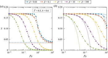
These effects are further explored in figure 10 which shows slip lengths for a range of $Pe$ and for different values of $\beta$ with $\bar {\varGamma } = 0.5$ and $b=0.6$. There is now a significant amount of surfactant on the interface. For $\beta =0.01$ another elbow can be seen in the graph, akin to that discussed earlier in the $\bar {\varGamma }=0.05$ case. However, this elbow now occurs at much smaller $Pe$ because even relatively weak advection causes the surfactant concentration to get close to its maximum. The slip lengths in this case are also reduced significantly compared with the smaller $\bar {\varGamma }$ cases. This is as expected because as $Pe\rightarrow \infty$ a stagnant cap should cover half of the domain for small $\beta$. To illustrate this, figure 11 shows the slip velocities and surfactant concentrations for $\beta =0.01$. In figure 11(b), the surfactant concentration reaches its ceiling even for Péclet numbers as low as $Pe=10$, causing significant surface immobilisation as evident in figure 11(a). Since $\bar {\varGamma }=0.5$ and $\beta$ is small, it is expected that as $Pe\rightarrow \infty$ the surfactant accumulates in a stagnant cap occupying half the meniscus. The surfactant concentration can be seen converging to the expected $Pe\rightarrow \infty$ and $\beta \rightarrow 0$ limit (5.25a–c). Figure 11(a) also shows an example of some numerical difficulties encountered at large values of $Pe$. As $Pe$ increases and a stagnant cap forms, a square-root singularity forms at the edge of the stagnant cap. Unlike those at the edges of the meniscus, this emergent square-root singularity is not resolved implicitly by the complex variable formulation, and the number of modes required for an accurate solution increases significantly. Specifically all runs with $Pe=1000$ were done with $N=150$ modes, whereas those for most other values required significantly fewer modes, with $N=10$ being sufficient for low $Pe$. It is evident from figure 11(a) that even $N=150$ struggles to fully resolve the stagnant-cap singularity, however increasing resolution further was found to reduce the size of the observed numerical oscillations. Adding to the challenge, these simulations at high $Pe$ required a full Newton solve. This culminated in an average of about 10 h per solution on a desktop PC which put a reasonable cap for the solutions at $Pe=1000$ due to time considerations. Such numerical challenges are, however, to be expected in view of the emergent singularity in the physical system. An interesting avenue of future research is to find a way to incorporate not only the edge-point singularities but also this emergent square-root singularity into the complex variable description to extend the range of the numerical simulation to even higher values of $Pe$. Nevertheless, that this simple method successfully resolved the system for Péclet numbers as high as the (physically relevant) value of $Pe=1000$ is noteworthy.

Figure 10.

(a) Slip length as a function of $Pe$ for different values of $\beta$ with $\bar {\varGamma } = 0.5$ and $b=0.6$. The horizontal dashed line corresponds to the $Pe\rightarrow \infty$ and $\beta \rightarrow 0$ limit (5.25a–c). (b) Refined view of the slip length curves for small $Pe$. The dotted lines are results given by (5.12).

Figure 11.

(a) Slip velocity profiles and (b) surfactant concentrations for different $Pe$ with $\bar {\varGamma } = 0.5$, $b=0.6$ and $\beta =0.01$. The vertical dashed line in (b) corresponds to the $Pe\rightarrow \infty$ and $\beta \rightarrow 0$ limit (5.25a–c).

When $\beta$ is larger, it is less common to reach maximum packing because surfactant gradients tend to be smaller. Figure 12 shows slip velocities and surfactant concentrations for $\beta =1$. At this relatively large $\beta$ the balance of surface diffusion and convection is such that the total surfactant concentration does not reach $1$ anywhere in the domain. However, the Marangoni stresses are sufficiently large to completely immobilise the meniscus for high $Pe$ values. Finally, figure 13 shows the slip velocities and surfactant concentrations for $\beta =100$. The slip velocities rapidly shrink to zero as $Pe$ is increased. Moreover, because $\beta$ is large the surfactant concentration converges to $\varGamma = \bar {\varGamma }+x(1-\bar {\varGamma })/\beta$. And because $\bar {\varGamma }$ is also large, immobilisation begins to occur when $Pe$ is of order unity. This is because, although small $Pe$ generally yields almost uniform surfactant concentrations, at high enough values of $\beta$ and $\bar {\varGamma }$ even small surfactant gradients at low $Pe$ cause Marangoni stresses large enough to immobilise the meniscus.

Figure 12.

(a) Slip velocity profiles and (b) surfactant concentrations for different $Pe$ with $\bar {\varGamma } = 0.5$, $b=0.6$ and $\beta =1$.

Figure 13.

(a) Slip velocity profiles and (b) surfactant concentrations for different $Pe$ with $\bar {\varGamma } = 0.5$, $b=0.6$ and $\beta =100$.

8.2. Effect of $\beta$

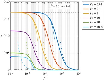
Also of interest is an exploration of how changing $\beta$ affects the flow. Figure 14 shows the slip length, now as a function of $\beta$, for various values of $Pe$ with $b=0.6$ and $\bar {\varGamma }=0.005$. This figure also shows results from the perturbation analysis for small $\beta$ given in § 5.2 and from the slip length approximation

(8.2)\begin{equation} \lambda \approx \frac{b }{a}\frac{(1- \hat \varGamma_0) }{\beta Pe \hat \varGamma_0},\end{equation}

derived in (B11) from a large-$\beta$ analysis given in Appendix B.

Figure 14.

Slip length as a function of $\beta$ for different values of $Pe$ with $b=0.6$ and $\bar {\varGamma }=0.005$. The dotted lines beginning at the top of the figure are from the small $\beta$ analysis (5.23). The dashed lines towards the bottom of the figure are from (8.2).

As $\beta \rightarrow 0$, the slip lengths all converge to that of a shear-free meniscus and the perturbation analysis of § 5.2 provides a good approximation as long as $Pe$ is order unity or below, which ensures (5.24) is sufficiently small. In fact, for $Pe=0.01$, there is agreement between the perturbation results and the numerical results up to about $\beta = 10^4$. At larger $\beta$ the approximation (8.2) matches closely with the numerical results. The slip length vanishes as $\beta$ increases, regardless of $Pe$, which is expected because eventually $\beta$ becomes large enough to cause stresses that immobilise the meniscus.

Another interesting effect seen in figure 14 is that because $\bar {\varGamma }$ is small, the effects of $\beta$ on the flow are weak: indeed very large values of $\beta$ are needed to fully immobilise the meniscus. When $\bar {\varGamma }$ is larger, smaller values of $\beta$ are enough to cause immobilisation. To show this, figure 15 shows the slip length, now as a function of $\beta$, for various values of $Pe$ with $b=0.6$, but now for the larger value $\bar {\varGamma }=0.05$. Qualitatively, the results appear similar, with the general shape of the curves looking the same. But the values of $\beta$ necessary to immobilise the meniscus are reduced by an order of magnitude. This is because the steady state surfactant concentrations for increased amounts of surfactants necessarily have larger gradients, so that a smaller $\beta$ can create the same stress. 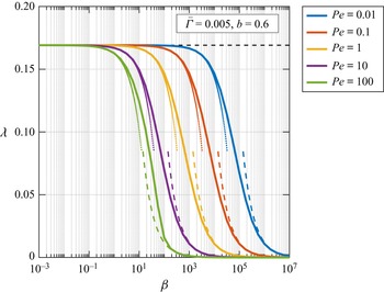One thing that the cases $\bar {\varGamma }=0.005$ and $\bar {\varGamma }=0.05$ have in common is that the surfactant level does not reach maximum packing for these values of $Pe$; however, if we increase $\bar {\varGamma }$ even further to $\bar {\varGamma }=0.5$, the nonlinearity of the equation of state has a major effect. Figure 16 shows the slip length, now as a function of $\beta$, for various values of $Pe$ with $b=0.6$ and $\bar {\varGamma }=0.5$. As $Pe$ increases, the slip lengths no longer converge to those associated by the fully shear-free meniscus. Instead the solutions converge to steady-state flows, dependent on $Pe$, where part of the meniscus is fully immobilised. This is because of the nonlinearity in the Langmuir equation of state and is consistent with theoretical observations made in § 5.2. For sufficiently small $Pe$ ($Pe =1$ or lower in figure 16) the numerical results agree well with the perturbation analysis as indicated by the dotted lines; perturbation results for higher $Pe$ are not shown because the agreement is poor. As $Pe$ increases diffusion weakens, whereas as $\beta$ decreases Marangoni forces weaken. The cumulative effect is that surfactants are free to be swept downstream, accumulating in stagnant caps in near-maximally packed regions where $\varGamma \approx 1$. The blue cross on the axis in figure 16 indicates the slip length value appropriate when $Pe\rightarrow \infty$ and $\beta \rightarrow 0$ as given by (5.25a–c); the slip length at $Pe=1000$, $\beta =0.001$ is already close to this value. Figure 17 shows velocity profiles for $\beta$ values significantly greater than unity; these plots correspond to the flows shown earlier in figure 14. The dashed lines in figure 17 refer to estimates for the velocity from large-$\beta$ analysis in Appendix B given by

(8.3)\begin{equation} U = \frac{(1- \hat \varGamma_0) }{\beta Pe \hat \varGamma_0},\end{equation}

and derived in (B10a,b). Figure 17(a), where $Pe=1$, is a regime where the flow is partially retarded at $\beta =10^2$ and becomes severely retarded as $\beta$ grows. The approximation (8.3) does a poor job at $\beta =10^2$, and leads to severe overestimation of the slip lengths. However, as $\beta$ increases formula (8.3) becomes increasingly accurate. Figure 17(b), for which $Pe=100$, shows a regime where the flow is nearly fully immobilised; here the approximation (8.3) is in excellent agreement with the velocity profiles. Interestingly, the velocities take on a top-hat shape where velocity assumes a near constant value along most of the interior of the meniscus before rapidly dropping off to zero at the edges.

Figure 15.

Slip length as a function of $\beta$ for different values of $Pe$ with $b=0.6$ and $\bar {\varGamma }=0.05$. The dotted lines beginning at the top of the figure are from the small $\beta$ analysis (5.23). The dashed lines towards the bottom of the figure are from (8.2).

Figure 16.

Slip length as a function of $\beta$ for different values of $Pe$ with $b=0.6$ and $\bar {\varGamma }=0.5$. The dotted lines beginning at the top of the figure are from the small $\beta$ analysis (5.23). The dashed lines towards the bottom of the figure are from (8.2). The blue cross marks the slip length from the $Pe\rightarrow \infty$ and $\beta \rightarrow 0$ limit (5.25a–c).

Figure 17.

Slip velocity profiles for different (large) $\beta$ with (a) $Pe=1$ and (b) $Pe = 100$ for $\bar {\varGamma } = 0.05$, $b=0.6$. Dotted lines show the approximation (B10a,b) of the slip velocity.

Concerning the effects of the geometry of the surface, results have been presented here, across the range of surface Péclet, Marangoni numbers and surfactant loads for the particular surface geometry with $b=0.6,\ a=1$, but a suite of similar calculations were carried out for $b=0.8$ and showed qualitatively similar results to those already described.