1. Introduction
Particle-laden thermal turbulence is very common in various nature and industrial processes. Examples include the interaction between clouds and radiation (Shaw Reference Shaw2003), fluidised bed combustion (Wen et al. Reference Wen, Ferraro, Nicolai, Hashimoto, Hayashi, Nakatsuka, Tainaka and Hasse2023), and particle solar receivers (Miller & Koenigsdorff Reference Miller and Koenigsdorff2000). In a solar receiver, the falling particles are used as the better absorber of radiation than the working fluid. After absorbing the radiation energy, they can transfer the heat to the working fluid efficiently. Similarly, cirrus clouds are warmed through the absorption of infrared radiation by ice particles, which produce upward vertical fluid motion (Durran et al. Reference Durran, Dinh, Ammerman and Ackerman2009). These updrafts are sometimes stronger than the terminal velocity of the ice particles, indicating the possibility of maintaining clouds consisting of very small crystals against sedimentation. The dynamic coupling between particles and thermal turbulence is important in these processes, and it can decelerate particles settling or drive particles upwards.
The coupling mechanisms introduced by the particles include momentum coupling, thermal coupling and interaction between the particles. The volume fraction of particles
 $\varPhi _V$
is a very important parameter to describe the interphase coupling of two phases. When
 $\varPhi _V$
is approximately equal to or less than
 $10^{-3}$
, the interaction between particles can be ignored, and one usually uses either the one-way or two-way coupling model (Elghobashi Reference Elghobashi1994; Balachandar & Eaton Reference Balachandar and Eaton2010; Brandt & Coletti Reference Brandt and Coletti2022).
Many studies have been conducted by considering the momentum couplings between particles and turbulent flows. Turbulent transport tends to trigger clustering particles, as evidenced by numerous experimental, numerical and theoretical studies. One of the primary mechanisms is the centrifugal effect. Inertial particles preferentially accumulate in regions of low vorticity due to ejection from coherent vortical structures (Squires & Eaton Reference Squires and Eaton1991). In homogeneous turbulence, the sweep-stick mechanism provides a conceptual framework for understanding the clustering of inertial particles. It suggests that particles tend to stick to regions of zero fluid acceleration, which are swept and clustered by large-scale motions (Chen, Goto & Vassilicos Reference Chen, Goto and Vassilicos2006; Petersen, Baker & Coletti Reference Petersen, Baker and Coletti2019).
In wall-bounded turbulence, particles tend to drift towards low-speed streaks near the wall due to fluctuations in the wall-normal velocity, a phenomenon known as turbophoresis (Johnson, Bassenne & Moin Reference Johnson, Bassenne and Moin2020). This effect has been widely studied, with one of the earliest contributions by Caporaloni et al. (Reference Caporaloni, Tampieri, Trombetti and Vittori1975). Theoretical analysis by Reeks (Reference Reeks1983) established the relationship between the net particle flux and the particle velocity skewness. In a more recent study, Nowbahar et al. (Reference Nowbahar, Sardina, Picano and Brandt2013) proposed an analytical model suggesting that the turbophoretic drift is reduced because the wall-normal variation of the wall-normal fluid velocity fluctuations decreases. Besides, the particle migration towards the centre of the channel (pipe) as a result of the Saffman effect was observed in both experiments (Oliveira, van der Geld & Kuerten Reference Oliveira, van der Geld and Kuerten2017; Shokri et al. Reference Shokri, Ghaemi, Nobes and Sanders2017) and numerical simulation (Zhu et al. Reference Zhu, Yu, Pan and Shao2020; Yu et al. Reference Yu, Xia, Guo and Lin2021). Yu et al. (Reference Yu, Xia, Guo and Lin2021) studied the particle-laden turbulent flows in an upward vertical channel, and found that in the near-wall region, the large Saffman lift force leads to a very small particle volume fraction.
In addition to modifying the spatial distribution of the particles, particle–turbulence interactions also influence the settling or rising velocity of the particles. In such flows, heavy particles settling under gravity may impose a non-negligible collective drag on the carrier fluid. This effect, along with preferential sweep, contributes to an increased particle settling rate (Bosse, Kleiser & Meiburg Reference Bosse, Kleiser and Meiburg2006). The particle clusters are elongated and preferentially aligned with gravity (Ireland, Bragg & Collins Reference Ireland, Bragg and Collins2016; Baker et al. Reference Baker, Frankel, Mani and Coletti2017). The sizes of clusters are extended to integral scale of the flow, which can induce vortical structures across a broad spectrum of scales (Kajishima & Takiguchi Reference Kajishima and Takiguchi2002; Petersen et al. Reference Petersen, Baker and Coletti2019). Similarly, the rise velocity of light particles is reduced in turbulent flow compared to stationary fluid. The shear-induced lift force tends to transport bubbles towards down-flow regions, which increases relative velocity and viscous drag (Mathai, Lohse & Sun Reference Mathai, Lohse and Sun2020).
Beyond the momentum couplings, the thermal couplings also exert significant influence on the two phases. A typical model is particle-laden Rayleigh–Bénard convection (RBC), which is driven by temperature difference. By modifying local temperature fluctuations and fluid density, the particles alter the flow structure, which in turn influences their behaviour. For example, it has been reported in RBC that the settling velocity and preferential concentration of the particles are strongly influenced by the momentum and thermal couplings with convection (Oresta & Prosperetti Reference Oresta and Prosperetti2013; Park, O’Keefe & Richter Reference Park, O’Keefe and Richter2018; Yang et al. Reference Yang, Zhang, Wang, Dong and Zhou2021). Oresta & Prosperetti (Reference Oresta and Prosperetti2013) revealed that the particles are swept up and accumulated in the descending stream in RBC. Yang et al. (Reference Yang, Zhang, Wang, Dong and Zhou2021) found that the settling velocity of the particles exhibits a power-law relationship with the Rayleigh number, which characterises the strength of thermal convection. Meanwhile, preferential concentration of particles also affects the momentum and heat exchange between particles and fluid (Pouransari & Mani Reference Pouransari and Mani2017, Reference Pouransari and Mani2018; Rahmani et al. Reference Rahmani, Geraci, Iaccarino and Mani2018).
Besides the large-scale temperature gradient, the forcing field can also come from heated particles. The particles absorb radiation and release heat to the surrounding fluid, leading to the appearance of turbulent thermal convection. Such externally heated particles have been studied for several groups for homogeneous turbulence (Zamansky et al. Reference Zamansky, Coletti, Massot and Mani2014, Reference Zamansky, Coletti, Massot and Mani2016; Frankel et al. Reference Frankel, Pouransari, Coletti and Mani2016). Zamansky et al. (Reference Zamansky, Coletti, Massot and Mani2014, Reference Zamansky, Coletti, Massot and Mani2016) studied the self-sustained turbulence caused by radiative heating, where the gravity of the particles is neglected. The behaviours of turbulent kinetic and particle distributions were investigated with different particle inertias and radiation intensities. Frankel et al. (Reference Frankel, Pouransari, Coletti and Mani2016) considered particle settling by gravity, and studied the influence of particle heating and gravity on the settling velocity in homogeneous turbulence. The particle heating induces rising buoyant plumes, and leads to significant reduction of the mean settling velocity. The RBC with externally heated particles was studied very recently by several groups (Pan et al. Reference Pan, Dong, Zhou and Shen2022; Yang et al. Reference Yang, Wan, Zhou and Dong2022; Tang et al. Reference Tang, Pan, Yang and Dong2024), in which the convection is driven together by the temperature difference between the top and bottom boundaries and by the heated particles.
Here, we focus on vertically wall-bounded turbulence driven solely by heat-releasing particles that absorb energy from external sources. The current work can also be viewed as an extension of our previous works on the wall-bounded convection driven by heated particles in which the gravity is normal to the wall. In this configuration, the particles accumulate into the boundary layer in the specific parameter space, while for other cases, particles are constantly advected over the entire domain (Du & Yang Reference Du and Yang2022, Reference Du and Yang2023). Similarly, Chen et al. (Reference Chen, Liao, Lin, Wan, Gao, Liu and Lu2025) investigated thermal convection driven by heat-releasing particles in a three-dimensional cubic cavity, and identified three typical large-scale circulation states at different density ratios. For the present work, the direction of gravity is parallel to the wall. The competition between the gravitational effect on the particles and the buoyancy effect on the fluid determines whether the motion of the two phases is upwards or downwards. These two effects are characterised by the Rayleigh number and the Froude number, respectively. We are interested in identifying the critical Froude number for different Rayleigh numbers under which particles and fluid transit from a settling regime to a buoyancy-driven rising regime.
The rest of the paper is organised as follows. In § 2, we provide the governing equations, the key parameters and the numerical details. Section 3 discusses the transport behaviours, and § 4 discusses the preferential concentration of particles. Conclusions are given in § 5.
2. Governing equations and numerical methods
2.1. Governing equations and key parameters
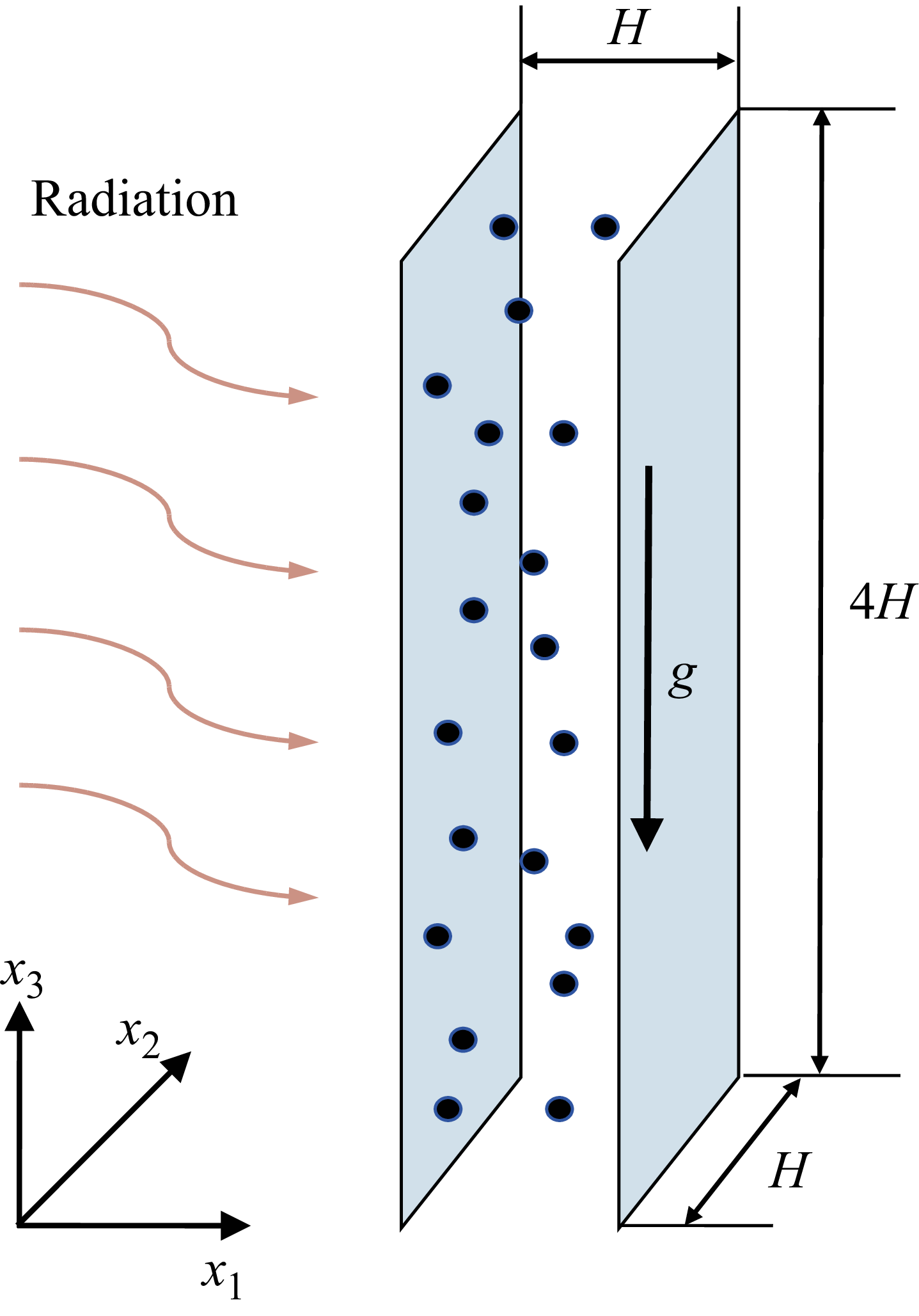
We consider a fluid layer confined between two vertical plates that are separated by a distance
 $H$
and are parallel to the direction of gravity. A schematic diagram of the vertical channel is depicted in figure 1. The computation domain is
 $[0,H]\times [0,H]\times [0,4H]$
in the wall-normal (
 $x_1$
), spanwise (
 $x_2$
) and vertical (
 $x_3$
) directions, respectively. The dispersed solid particles are carried by the fluid phase. The fluid density is assumed to vary linearly with temperature as
 $\rho = \rho _0(1 - \alpha \theta )$
, where
 $\rho _0$
is the reference-state density,
 $\theta = T - T_0$
denotes the temperature deviation from the reference temperature
 $T_0$
, and
 $\alpha$
is the thermal expansion coefficient. The two plates are maintained at the same constant temperature
 $T_0$
, corresponding to the reference state. Under the Oberbeck–Boussinesq approximation, the density variations are assumed to be small and only retained in the buoyancy term. Then the governing equations for the fluid phase read
 \begin{align} \boldsymbol{\nabla }\boldsymbol{\cdot }\boldsymbol{u}^* &= 0, \\[-12pt] \nonumber \end{align}
 \begin{align} \partial ^*_t\boldsymbol{u^*} + \boldsymbol{u}^*\boldsymbol{\cdot }\boldsymbol{\nabla }^*\boldsymbol{u}^*&= - \boldsymbol{\nabla }^* p^* + \nu \,{\nabla} ^{*2} \boldsymbol{u}^* + g \alpha \theta ^* \boldsymbol{e}_z + \boldsymbol{f}^*, \\[-12pt] \nonumber \end{align}
 \begin{align} \partial ^*_t\theta ^* + \boldsymbol{u^*}\boldsymbol{\cdot }\boldsymbol{\nabla }^*\theta ^* &= \kappa\, {\nabla} ^{*2} \theta ^* + q^*. \\[10pt] \nonumber \end{align}
Here,
 $\boldsymbol{u}=(u_1,u_2,u_3)$
denotes the fluid velocity vector,
 $p$
represents kinematic pressure,
 $\nu$
is kinematic viscosity,
 $g$
is gravitational acceleration, and
 $\kappa$
is the thermal diffusivity. The extra source term
 $\boldsymbol{f}$
in (2.1b
) accounts for the feedback force of the particle phase on the fluid phase. The feedback heat flux is denoted by
 $q$
in (2.1c
). Hereafter, the asterisk superscript indicates dimensional quantities or operators. It is worth noting that turbulence is sustained solely by particle-induced terms, with no additional external forcing.
Schematic diagram of the vertical channel flow laden with heated particles.

In the present work, the particle size is assumed to be smaller than the Kolmogorov scale. Thus the Lagrangian point-particle method is used to track the motion and temperature of the particles. The particle Biot number is less than 0.1 in all cases, resulting in a homogeneous particle temperature. The full set of particle equations in the present study reads
 \begin{align} \frac {\mathrm{d}\boldsymbol{x}^*_p}{\text{d}t^*}&=\boldsymbol{u}^*_p, \\[-12pt] \nonumber \end{align}
 \begin{align} \frac {\mathrm{d}\boldsymbol{u}^*_p}{\text{d}t^*}&= C_D\frac {\boldsymbol{u}^*_f-\boldsymbol{u}^*_p}{\tau _p} - g \left(1-\frac {\rho _0}{\rho _p}\right)\boldsymbol{e}_z + C_L \frac {\rho _0}{\rho _p} \big[\big(\boldsymbol{u}^*_f-\boldsymbol{u}^*_p \big) \times \boldsymbol \omega _{\kern-1pt f}^* \big], \\[-12pt] \nonumber \end{align}
 \begin{align} \frac {\mathrm{d}\theta ^*_p}{\text{d}t^*}&= \frac {\textit{Nu}_p}{2}\frac {\theta ^*_f-\theta ^*_p}{\tau _\theta }+\frac {\phi ^*_p}{m_p c_p}. \\[10pt] \nonumber \end{align}
Here, the subscript
 $p$
denotes the quantity related to the particle,
 $f$
denotes the fluid quantity at the same location of the particle, and
 $\boldsymbol \omega$
is the fluid vorticity vector. As can be seen from (2.2b
), forces acting on the particles include the Stokes drag force, the gravity force and the Safffman lift force. Here,
 $C_D$
represents the drag correction coefficient, which is defined as
 $C_D=1+0.15\,Re_p^{0.678}$
. The particle Reynolds number is
 $ \textit{Re}_p= d_p | \boldsymbol{u}^*_f-\boldsymbol{u}^*_p | / \nu$
. Considering the large velocity gradient, the Saffman lift force should also be considered. Based on the Saffman–Mei model (Saffman Reference Saffman1956; Mei Reference Mei1992), the Saffman lift coefficient
 $C_L$
is
 \begin{align} C_L=\frac {9.69}{\pi \sqrt {Re_{\omega }}}f_{\textit{mei}}, \end{align}
with
 \begin{align} f_{\textit{mei}}& =(1-0.3314 \chi ^{0.5})\,{\rm e}^{-Re_p/10} +0.3314\chi ^{0.5}, \quad Re_p\le 40, \\[-12pt] \nonumber \end{align}
 \begin{align} f_{\textit{mei}}& =0.0524 (\chi\, Re_p)^{0.5}, \quad Re_p \gt 40. \\[10pt] \nonumber \end{align}
Here,
 $\chi = Re_{\omega } / (2\, Re_p)$
is the ratio between the vorticity Reynolds number
 $ \textit{Re}_{\omega } = | \omega |\, d_p^2/ \nu$
and the particle Reynolds number.
The two terms on the right-hand side of (2.2c
) account for the heat exchange between the two phases and the heating rate by an external energy source. Here,
 $\phi _p$
and
 $m_p$
denote the power of external energy input and the mass of a single particle, respectively. Two typical time scales are evolved in (2.2b
) and (2.2c
). The Stokes time is defined as
 $\tau _p=\rho _p d^2_p/\rho _0 18\nu$
, with
 $d_p$
being the particle diameter. The temperature Stokes time is approximated by the relaxation of the particle temperature towards the fluid temperature with the time scale
 $\tau _\theta =(3/2)(\nu /\kappa )(c_p/c_{\kern-1pt f})\tau _p$
(Zamansky et al. Reference Zamansky, Coletti, Massot and Mani2016), where
 $c_p$
and
 $c_{\kern-1pt f}$
are the heat capacities of the solid particle and fluid.
The source terms in (2.1b ) and (2.1c ) can be calculated by the Stokes drag force and the Saffman lift force in (2.2b ), and the thermal relaxation term in (2.2c ), respectively. In the Eulerian description of the fluid phase, the particle-induced source terms are expressed using the Dirac delta distribution:
 \begin{align} \boldsymbol{f}^* &= - \frac {1}{\rho _0} \sum _p^{N_p} m_p\left[C_D\frac {\boldsymbol{u}^*_f-\boldsymbol{u}^*_p}{\tau _p} + C_L \frac {\rho _0}{\rho _p} \big(\boldsymbol{u}^*_f-\boldsymbol{u}^*_p \big) \times \boldsymbol \omega _{\kern-1pt f}^* \right]\delta \big(\boldsymbol{x^*}-\boldsymbol{x}^*_p \big), \\[-12pt] \nonumber \end{align}
 \begin{align} q^* &= - \frac {1}{\rho _0c_{\kern-1pt f}}\sum _p^{N_p} m_p c_p \frac {\theta ^*_f-\theta ^*_p}{\tau _{\theta }} \,\delta \big(\boldsymbol{x^*}-\boldsymbol{x}^*_p \big). \\[10pt] \nonumber \end{align}
The procedure of non-dimensionalisation has already been given in detail in our previous work (Du & Yang Reference Du and Yang2022). In the current work, we will briefly introduce the characteristic scales. The characteristic length scale is selected as the horizontal distance of the domain
 $H$
, the temperature scale as
 $\varDelta _T = (n_p^2 \phi _p^2 H/g \alpha \rho _0^2 c_{\kern-1pt f}^2)^{1/3}$
, the velocity scale as
 $U_{\mathit{ff}} = (g \alpha n_p \phi _p H^2 / \rho _0 c_{\kern-1pt f} )^{1/3}$
, and the time scale as
 $\tau _f = H / U_{\mathit{ff}}$
, where
 $n_p$
is the particle number density. Using the above characteristic scales, the non-dimensional governing equations can be readily obtained as
 \begin{align} \boldsymbol{\nabla }\boldsymbol{\cdot }\boldsymbol{u}&=0, \\[-12pt] \nonumber\end{align}
 \begin{align} \partial _t\boldsymbol{u}+ \boldsymbol{u}\boldsymbol{\cdot }\boldsymbol{\nabla }\boldsymbol{u} &= - \boldsymbol{\nabla } p + Ra^{-1/3}Pr^{2/3}\,{\nabla} ^2 \boldsymbol{u} + \theta \boldsymbol{e}_z + \boldsymbol{f}, \\[-12pt] \nonumber\end{align}
 \begin{align} \partial _t\theta + \boldsymbol{u}\boldsymbol{\cdot }\boldsymbol{\nabla }\theta &= Ra^{-1/3}\,Pr^{-1/3}\,{\nabla} ^2 \theta + q, \\[-12pt] \nonumber\end{align}
 \begin{align} \mathrm{d}_t \boldsymbol{x}_p&=\boldsymbol{u}_p, \\[-12pt] \nonumber\end{align}
 \begin{align} \mathrm{d}_t \boldsymbol{u}_p&=C_D\frac { \boldsymbol{u}_{\kern-1pt f}-\boldsymbol{u}_p}{St} - \frac {\boldsymbol{e}_z}{Fr^2} + C_L \frac {\rho _0}{\rho _p} (\boldsymbol{u}_{\kern-1pt f}-\boldsymbol{u}_p) \times \boldsymbol \omega _{\kern-1pt f}, \\[-12pt] \nonumber\end{align}
 \begin{align} \mathrm{d}_t \theta _p&=\frac {\textit{Nu}_p}{2}\frac {\theta _f-\theta _p}{St_T}+\frac {1}{\varPhi _{\theta }}, \\[10pt] \nonumber\end{align}
with
 \begin{align} \boldsymbol{f}&= -\sum _p^{N_p} \frac {\varPhi _V}{C} \frac {\rho _p}{\rho _0} \left[C_D\frac { \boldsymbol{u}_{\kern-1pt f}-\boldsymbol{u}_p}{St} + C_L \frac {\rho _0}{\rho _p} (\boldsymbol{u}_{\kern-1pt f}-\boldsymbol{u}_p) \times \boldsymbol \omega _{\kern-1pt f}\right] \delta (\boldsymbol{x}-\boldsymbol{x}_p), \\[-12pt] \nonumber \end{align}
 \begin{align} q &= -\sum _p^{N_p} \frac {\varPhi _V}{C} \frac {\rho _p}{\rho _0} \frac {c_p}{c_{\kern-1pt f}} \frac {\textit{Nu}_p}{2} \frac {\theta _f-\theta _p}{St_T}\,\delta (\boldsymbol{x}-\boldsymbol{x}_p). \\[10pt] \nonumber \end{align}
The boundary conditions for the fluid phases at the two plates are, in non-dimensional form,
 \begin{align} \boldsymbol{u}=\boldsymbol{0}, \ \theta =0 \quad \mbox{at}\ x_1=0, \\[-12pt] \nonumber \end{align}
 \begin{align} \boldsymbol{u}=\boldsymbol{0}, \ \theta =0 \quad \mbox{at} \ x_1=1. \\[10pt] \nonumber \end{align}
We employ an elastic reflection for the particles on the two plates. During particle–wall collisions, heat exchange between the particles and the wall is neglected. In the vertical and spanwise directions, the periodic boundary conditions are employed for all the flow and particle quantities.
Key control parameters include the Prandtl number
 $ \textit{Pr}$
, the Rayleigh number
 $ Ra$
, the Froude number
 $ \textit{Fr}$
, the Stokes number
 $ St$
, the density and heat capacity ratios between two phases, and the volume fraction of particles, which are defined as, respectively,
 \begin{eqnarray} && \textit{Pr}=\frac {\nu }{\kappa }, \quad Ra=\frac {g\alpha n_p \phi _p H^5}{\nu \kappa ^2 \rho _0 c_{\kern-1pt f}}, \quad \textit{Fr}=( \textit{Ra} \textit{Pr})^{1/3}\left (\frac {\kappa ^2}{g\left (1-\rho _0/\rho _p\right )H^3}\right )^{1/2}, \nonumber \\ && St = \frac {\tau _p}{\tau _f}, \quad \frac {\rho _p}{\rho _0}, \quad \frac {c_p}{c_{\kern-1pt f}} , \quad \varPhi _V=\frac { n_p \pi d_p^3 }{6}. \end{eqnarray}
Here,
 $ \textit{Ra}$
represents the ratio of the thermal buoyancy force to the viscosity force. The Froude number
 $ \textit{Fr}$
accounts for the ratio of the gravitation acceleration scale
 $g (1-\rho _0/\rho _p )$
of the particles to the buoyancy-induced fluid acceleration scale
 $U_{\kern-1pt \textit{ff}}/\tau _f$
. The Stokes number
 $ \textit{St}$
is the ratio of the particle relaxation time
 $\tau _p$
to the characteristic time
 $\tau _f$
of flow. From these parameters, the non-dimensional particle number density
 $C$
, particle thermal Stokes number
 $ \textit{St}_T$
, mass fraction of the particles
 $\varPhi _M$
and heat-capacity ratio
 $\varPhi _{\theta }$
can be obtained as
 \begin{eqnarray} && C= n_p H^3 = \sqrt {\frac {\varPhi _V^2 \textit{Ra} \rho _p^3}{162 \textit{St}^3 \pi ^2 \textit{Pr}^2 \rho _0^3}} , \quad \textit{St}_T=\frac {3 \textit{Pr} c_p \textit{St}}{2 c_{\kern-1pt f}} ,\nonumber \\ && \varPhi _M = \varPhi _V \frac {\rho _p}{\rho _0}, \quad \varPhi _{\theta }=\varPhi _M \frac {c_p}{c_{\kern-1pt f}}. \end{eqnarray}
The global responses of interest are the bulk Reynolds number
 $ \textit{Re}_b$
, the friction Reynolds number
 $ \textit{Re}_\tau$
, and the Nusselt number
 $ \textit{Nu}$
. The bulk Reynolds number
 $ \textit{Re}_b$
is defined as
 \begin{align} Re_b=\frac {\langle u_3^* \rangle _{V,t} H}{\nu }=\frac {\langle u_3 \rangle _{V,t} }{Ra^{-1/3}\, \textit{Pr}^{2/3}}, \end{align}
where
 $\langle {\cdot }\rangle _{V,t}$
denotes the average over the flow domain and time. The friction Reynolds number
 $ \textit{Re}_\tau$
is defined as
 \begin{align} Re_\tau =\frac {u_{\tau } H}{2\nu }. \end{align}
Here,
 $u_{\tau }=\sqrt {\tau _w/\rho }$
, with
 $\tau _w$
being the mean shear stress on the wall. Then the Nusselt number is defined as
 \begin{align} Nu=\frac {H}{6 \langle \theta ^* \rangle _V}\left (\frac {\mathrm{d} \overline {\theta ^*}}{\mathrm{d}x_1^*}\Bigg |_{x_1^*=0}-\frac {\mathrm{d} \overline {\theta ^*}}{\mathrm{d}x_1^*}\Bigg |_{x_1^*=H}\right )=\frac {1}{6 \langle \theta \rangle _V}\left (\frac { \mathrm{d} \overline {\theta }}{\mathrm{d}x_1}\Bigg |_{x_1=0} - \frac { \mathrm{d} \overline {\theta }}{\mathrm{d}x_1}\Bigg |_{x_1=1}\right ), \end{align}
where the overline denotes the average over time and the
 $x_2{-}x_3$
plane.
For the mean temperature, by taking the average of (2.8), we obtain
 \begin{align} \langle q \rangle _{V,t}=1. \end{align}
Then the spatial and temporal average of (2.6c ) leads to
 \begin{align} \frac { \mathrm{d} \overline {\theta }}{\mathrm{d}x_1}\Bigg |_{x_1=0} - \frac { \mathrm{d} \overline {\theta }}{\mathrm{d}x_1}\Bigg |_{x_1=1} = Ra^{1/3}\,Pr^{1/3}. \end{align}
Thus
 $ \textit{Nu}$
can be expressed as
 \begin{align} Nu=\frac {Ra^{1/3}\,Pr^{1/3} }{6 \langle \theta \rangle _{V,t}}. \end{align}
2.2. Numerical methods and parameter space
Direct numerical simulations with the point-particle model are carried out for the current flow. For the fluid phase, the governing equations (2.6a
)–(2.6c
) are discretised using the second-order finite-difference scheme with the fractional time step method, which is validated by convection and wall-bounded flow (Du & Yang Reference Du and Yang2022, Reference Du and Yang2023). The Lagrangian tracking of point particles is used to obtain the position, velocity and temperature of the particle. To compute the fluid velocities and temperature at particle locations, we use cubic Hermite spline interpolation. The source terms
 $f$
and
 $q$
are calculated by distributing towards the eight neighbouring Eulerian grids.
In this study, we consider the silicon carbide particle in air. Thus the Prandtl number is fixed at
 $ \textit{Pr}=0.7$
. The physical properties of the particles are
 $\rho _p/\rho _0 = 2469$
and
 $c_p/c_{\kern-1pt f}=1.15$
. In order to reduce the parameter space and focus on the interplay between particle gravity and the fluid buoyancy force, the Stokes number is fixed at
 $ \textit{St}=1$
and the volume loading is fixed at
 $\varPhi _V=2.3\times 10^{-3}$
. Three Rayleigh numbers are investigated,
 $ \textit{Ra}=10^6$
,
 $10^7$
and
 $10^8$
, and for each Rayleigh number, a series of Froude numbers is simulated over the range
 $0.4\lt \textit{Fr}\lt 10$
. As shown in (2.11), if all other control parameters are fixed, then
 $C \sim Ra^{1/2}$
, reaching
 $C=10^5$
at
 $ \textit{Ra}=10^8$
.
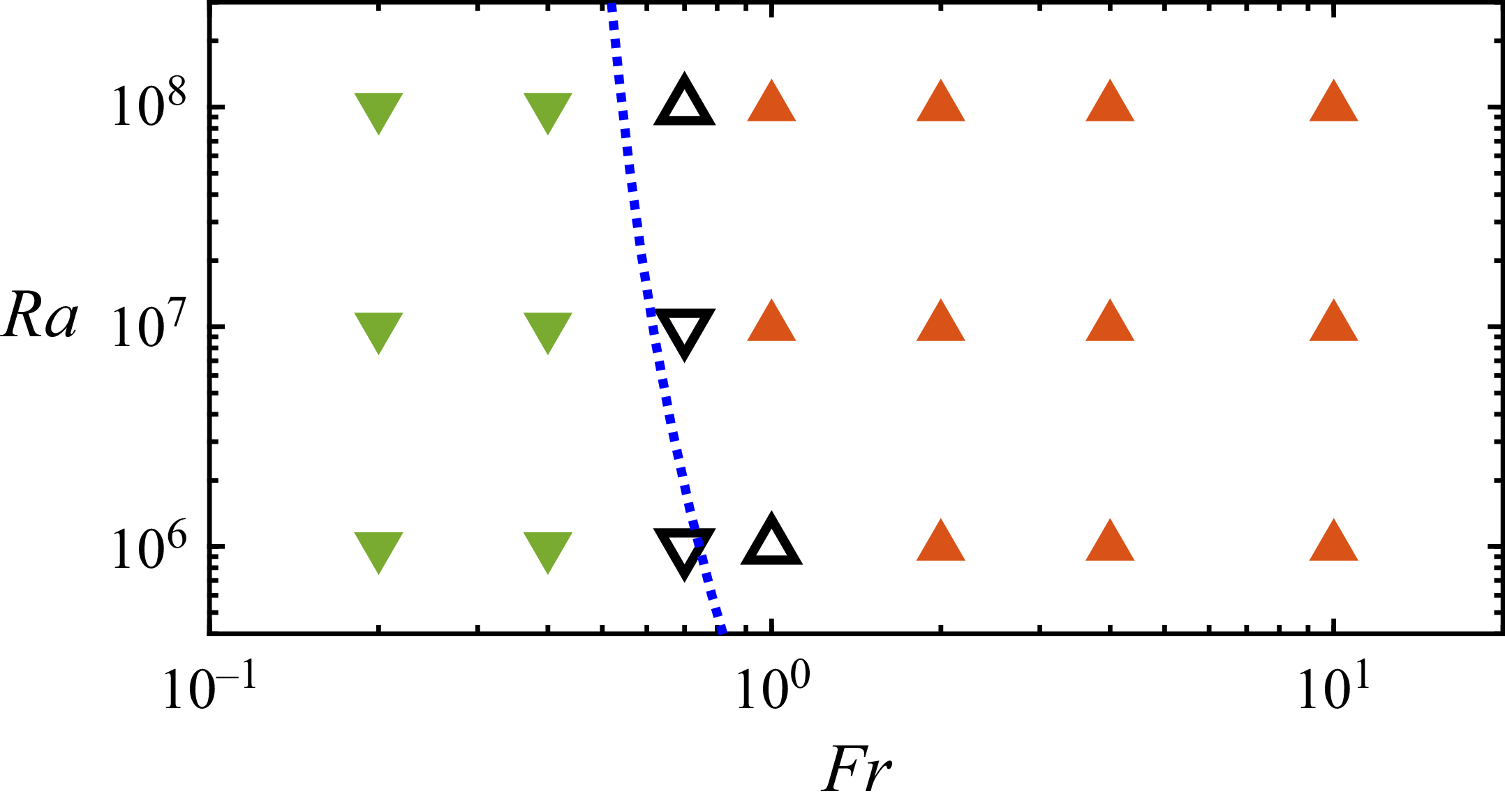
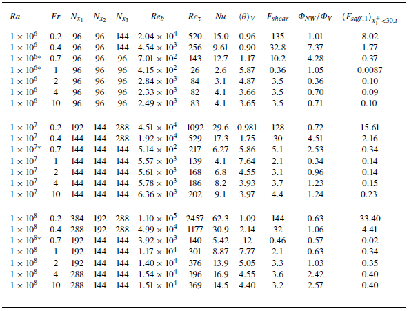
The explored parameter space is shown in figure 2, in which different types of symbols represent different flow regimes. When the Froude number is large enough, the fluid is driven upwards by the thermal buoyancy force and carries the particles, which are marked by orange up-pointing triangles. For cases with small Froude numbers, the falling particles drag the flow downwards, marked by the green down-pointing triangles. When the two driving forces are comparable with each other, the mean flow in the vertical direction is rather weak, and these cases are marked by the open symbols. We differentiate these cases from the upward or downward flowing cases by the criterion when the ratio of the volume-averaged mean vertical velocity is smaller than five times the magnitude of fluctuation velocity, i.e. the standard deviation of velocity magnitude. The critical parameters for the regime transition will be discussed in the next section. All the mean statistics will be discussed for the cases that exclude those near the regime transition. The details of numerical settings are given in table 1 in Appendix A.
The explored phase space in the
 $ \textit{Ra}{-}Fr$
plane at
 $ \textit{St}=1$
. The green down-pointing triangles represent the case in which all particles fall and induce downward flow. For those marked by orange up-pointing triangles, fluid carries particles upwards. The upward- and downward-pointing hollow triangles correspond to cases close to the regime transition, representing falling and rising regimes, respectively. The blue dashed line marks the scaling relations (3.14) and (3.15) for the critical Froude number.

To give some idea about the relation between the non-dimensional parameters and the real physical properties, we give an example of flow settings. For the case with
 $ \textit{Ra}=10^6$
and
 $ \textit{Fr}=0.2$
, one obtains
 $\phi _p=1.52\ \text{W}$
and
 $d_p=1.51\times 10^{-4}\, \text{m}$
. The particle diameter is very similar to values reported in Dritselis & Vlachos (Reference Dritselis and Vlachos2011). From these values, one can determine the incident radiation intensity
 $ W_{\textit{inlet}} = \phi _p/\pi d_p^2 \approx 2 \times 10^7 \ \text{W m}^{-2}$
, which is of the same order as reported in Kribus et al. (Reference Kribus, Doron, Rubin, Karni, Reuven, Duchan and Taragan1999).
3. Statistics of the fluid phase and transition of different regimes
3.1. The mean statistics of velocity and temperature
We first look at the mean statistics of the fluid phase. Figure 3 shows the vertically averaged mean profiles of vertical velocity for the cases with
 $ \textit{Ra}=10^8$
. Clearly, the velocity is symmetric about the centreline. The velocity profile has two distinct boundary layers adjacent to both plates, and in between there is a nearly homogeneous bulk region. As the Froude number increases, the vertical velocity undergoes a gradual reversal, transitioning from the downward (negative) to the upward (positive) stream, which is caused by the momentum coupling with the particles. As shown in figure 3(b), the profiles are compared with the law of the wall and the logarithmic law for fully developed single-phase turbulent channel flow without heat convection (Kim, Moin & Moser Reference Kim, Moin and Moser1987), where the superscript + denotes normalisation in wall units. In the viscous sublayer with
 $x_1^+\lt 5$
,
 $\overline {u_3^+}$
closely follows the linear law, while in the log-layer starting from
 $x_1^+\approx 30$
, the profiles exhibit a clear logarithmic scaling. The good agreement with both the near-wall law and the log-law indicates that the present flow has reached a statistically stationary and fully developed turbulent state.
Mean vertical velocity profiles for the cases with
 $ \textit{Ra}=10^8$
and different
 $ \textit{Fr}$
values: (a) in global coordinates; (b) in wall coordinates. The black dashed line denotes the classic mean velocity profile for single-phase well-developed channel flow.

Mean profiles for the cases with
 $ \textit{Ra}=10^8$
and different
 $ \textit{Fr}$
values: (a) standard deviation (std) of the vertical velocity; (b) standard deviation of the wall-normal velocity; (c) standard deviation of the spanwise velocity; (d) Reynolds shear stress.

Figures 4(a–c) display the fluctuation of three velocity components for the same cases as in figure 3. The effect of the Froude number
 $ \textit{Fr}$
on the three components is similar: they first decrease and then increase as
 $ \textit{Fr}$
increases, and the main stream changes from downwards to upwards. Meanwhile, the maxima of the three intensities move away from the wall and become broader. In figure 4(d), the profiles of Reynolds stress
 $\overline {u'_1u'_3}$
are plotted for different
 $ \textit{Fr}$
values. The variation trend of the Reynolds stress with increasing Froude number is consistent with that of the turbulence intensities.
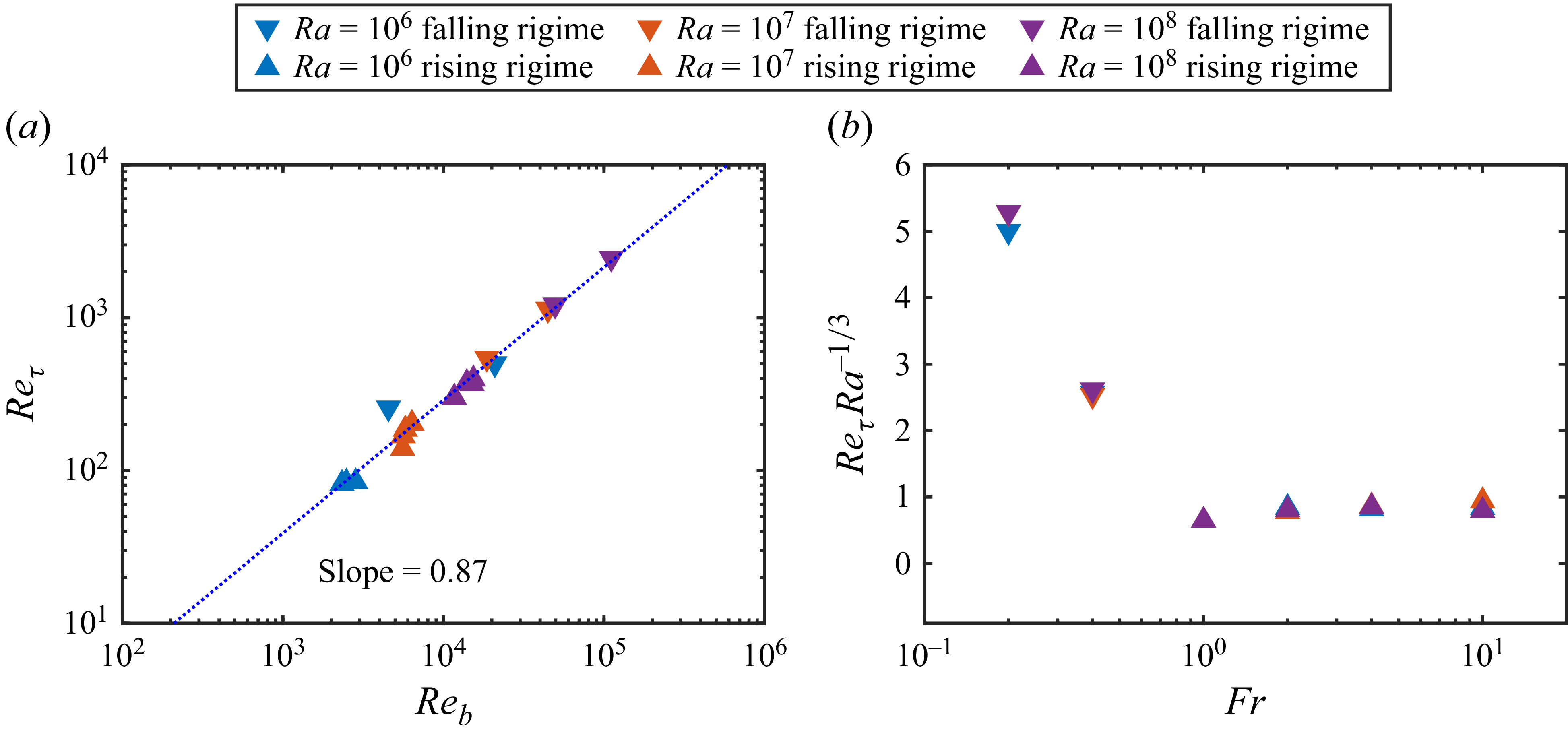
Then we turn to the relationship between the friction Reynolds number and the bulk Reynolds number. Figure 5(a) shows the variation of the friction Reynolds number versus the bulk Reynolds number. It is worth noting that both the falling and the rising regimes exhibit a similar power-law scaling
 $ \textit{Re}_\tau \sim Re_b^{0.87}$
, with the exponent determined by a fitting of numerical data. This exponent is very close to the value
 $0.875$
reported by Dean (Reference Dean1978) for the single-phase channel flow. In the turbulent channel flow, the relation between the friction Reynolds number and bulk Reynolds number can be expressed as
 $ \textit{Re}_b = 2\, Re_\tau\, \langle \overline {u_3^+}\rangle _{V,t}$
. Hence the relation is fully determined by the mean vertical velocity profile in wall units. As shown in figure 3, the profiles of mean vertical velocity
 $\overline {u_3^+}$
collapse onto the corresponding single-phase channel profile. Consequently,
 $\langle u_3^+ \rangle _{V,t}$
, and therefore the scaling between
 $ \textit{Re}_b$
and
 $ \textit{Re}_{\tau }$
, coincides with the single-phase turbulent channel flow.
(a) The friction Reynolds number
 $ \textit{Re}_{\tau }$
versus the bulk Reynold number
 $ \textit{Re}_b$
. The value of the slope comes from the least squares fit of the data. (b) Compensated plots of friction Reynolds number versus Froude number for different Rayleigh numbers.

Mean temperature velocity profiles for the cases with
 $ \textit{Ra}=10^8$
and different
 $ \textit{Fr}$
values: (a) in global coordinates; (b) in wall coordinates. The value of the Kármán constant comes from Kawamura et al. (Reference Kawamura, Ohsaka, Abe and Yamamoto1998). (c) The standard deviation of the temperature. (d) The turbulent heat flux.

Actually, the magnitude of
 $ \textit{Re}_\tau$
can be estimated as follows for a small enough Froude number. In the current system, three external forces are the particle gravity, the fluid buoyancy and the wall shear force. When
 $ \textit{Fr}$
is small, the particle gravity dominates the fluid buoyancy and is balanced mainly by the wall shear force. For the statistically steady state, the balance between the two forces gives
 \begin{align} F_{shear}=2\tau _w=\frac {\varPhi _M}{Fr^2}, \end{align}
which is readily obtained by integral of the momentum equation. Here,
 $F_{shear}$
stands for the wall shear force or the friction force. Then one has
 \begin{align} Re_{\tau } \approx \frac { \textit{Ra}^{1/3} \textit{Pr}^{-2/3}}{2\sqrt {2}} \sqrt {\frac {\varPhi _M}{Fr^2}}. \end{align}
For
 $ \textit{Ra}=10^8$
and
 $ \textit{Fr}=0.2$
, the above relation gives
 $ \textit{Re}_\tau \approx 2480$
, which is only slightly higher than the numerical value
 $ \textit{Re}_\tau =2457$
. This is reasonable since we ignore the buoyancy force, which is in the direction opposite to gravity. Another observation of (3.2) is that for a small Froude number,
 $ \textit{Re}_\tau \sim Ra^{1/3}$
. As shown in figure 5(b), the compensated value
 $ \textit{Re}_\tau\, Ra^{-1/3}$
changes with
 $ \textit{Fr}$
and is indepdent of
 $ \textit{Ra}$
. This indicates that
 $ \textit{Re}_\tau$
follows a single scaling law
 $ \textit{Re}_\tau \sim Ra^{1/3}$
with respect to
 $ \textit{Ra}$
for all Froude numbers.
Figure 6 presents the statistics of the temperature field and the turbulent heat flux in the wall-normal direction. As shown by the mean profiles in figure 6(a), the temperature near the channel centre is highest for intermediate Froude numbers with the smallest mean bulk velocity, and decreases as
 $ \textit{Fr}$
either increases or decreases. The reason is that at an intermediate Froude number, the turbulent intensity is weakest. Note that all the heat released by the particles has to be extracted from the system by the heat flux from the two walls. Weaker turbulent intensity results in smaller turbulent heat flux towards the side walls at channel centre, as indicated by figure 6(d).
Figure 6(b) plots the mean temperature profiles in the wall unit with
 $\overline {\theta ^+}=\overline {\theta }/\theta _{\tau }$
and
 $\theta _{\tau }= \kappa ({\rm d}\overline {\theta }_w/{\rm d}x_1)/{u_{\tau }}$
. The linear viscous sublayer and the log-layer are clearly visible, especially for those cases with large
 $ \textit{Re}_b$
. The slope of the log-layer is also consistent with that given by the Kármán constant,
 $\kappa _\theta =0.43$
(Kawamura et al. Reference Kawamura, Ohsaka, Abe and Yamamoto1998). As shown in figure 6(c), generally the temperature fluctuation also exhibits non-monotonic variation as
 $ \textit{Fr}$
increases, similar to the velocity fluctuation.
3.2. The transport properties and the global balance relations
When the flow is at rest, the heat transfer is dominated by the conduction between the bulk region and two vertical parallel plates. When the particle number density is high and the particles are randomly distributed, they can be treated as uniformly distributed across the fluid domain, leading to a uniform heat source. The governing equation for heat conduction can be deduced from (2.6c ) as
 \begin{align} {\nabla} ^2 \theta = -\textit{Ra}^{1/3} \textit{Pr}^{1/3}, \end{align}
and we arrive at the parabolic solution
 \begin{align} \overline {\theta }(x_1) = \textit{Ra}^{1/3} \textit{Pr}^{1/3}\, \big(x_1-x_1^2 \big). \end{align}
The bulk average temperature is
 \begin{align} \langle \theta \rangle _{V,Re_b=0}= \textit{Ra}^{1/3} \textit{Pr}^{1/3}/6. \end{align}
Thus when the flow is at rest, the bulk Reynolds equals zero and the non-dimensional heat flux at two boundaries, measured by the Nusselt number, can be obtained as
 \begin{align} \textit{Nu}_{Re_b=0}= 1 . \end{align}
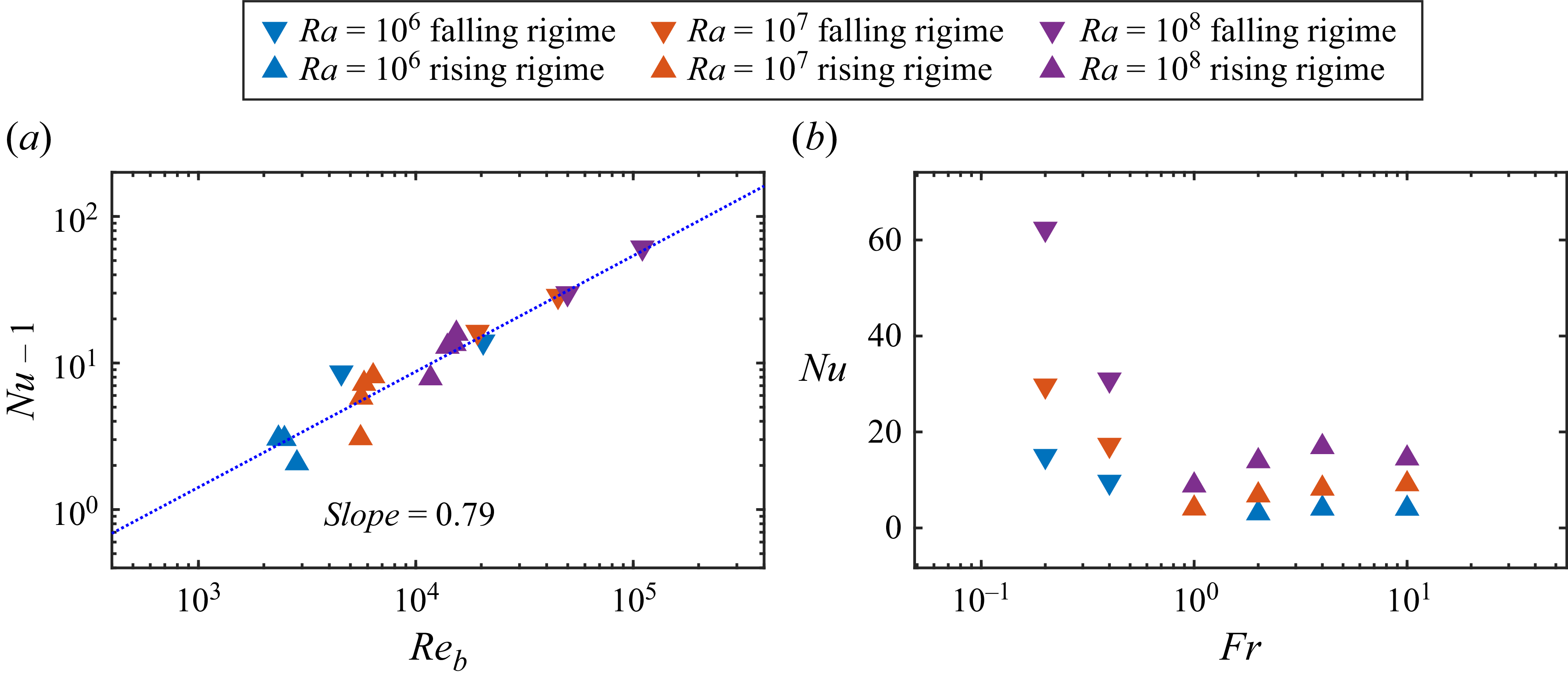
The Nusselt number is plotted in figure 7(a) versus the bulk Reynolds number
 $ \textit{Re}_b$
. A power-law scaling can be deduced from the data as
 $ \textit{Nu}-\textit{Nu}_{Re_b=0}=Nu-1\sim Re_b^{0.79}$
, which is close to the exponent found in single-phase channel turbulence (Dittus & Boelter Reference Dittus and Boelter1985). As shown in figure 7(b), the Nusselt number exhibits a non-monotonic dependence on the Froude number, initially decreasing and then increasing. In contrast, it increases monotonically with the Rayleigh number.
The Nusselt number
 $ \textit{Nu}$
versus (a) bulk Reynold number
 $ \textit{Re}_b$
and (b) Froude number
 $ \textit{Fr}$
. The value of the slope comes from the least squares fit of the data.

For buoyancy-driven flow, it is very useful to examine the exact global relations between flux and dissipation (Ahlers, Grossmann & Lohse Reference Ahlers, Grossmann and Lohse2009). For the current system, such relations can also be constructed as for turbulence convection with point particles (Yang et al. Reference Yang, Zhang, Wang, Dong and Zhou2021). By taking the inner product of the velocity with (2.6b ) and that of the temperature with (2.6c ), one readily obtains, respectively,
 \begin{align} \epsilon _u = \nu\, \big\langle (\partial _i^* u_{\kern-1pt j}^*)^2 \big\rangle _V = \frac {\nu ^3}{H^4}\, Ra\, \textit{Pr}^{-2}\, \left(\langle u_1\theta \rangle _{V,t} + \langle u_{\kern-1pt j} f_j \rangle _{V,t}\right), \\[-28pt] \nonumber\end{align}
 \begin{align} \epsilon _{\theta } = \kappa _T \big\langle (\partial _i^* \theta ^*)^2 \big\rangle _V = \frac {\kappa _T^5}{g^2 \alpha ^2 H^8}\, Ra^{5/3}\, \textit{Pr}^{5/3}\, \langle q\theta \rangle _{V,t}. \\[0pt] \nonumber \end{align}
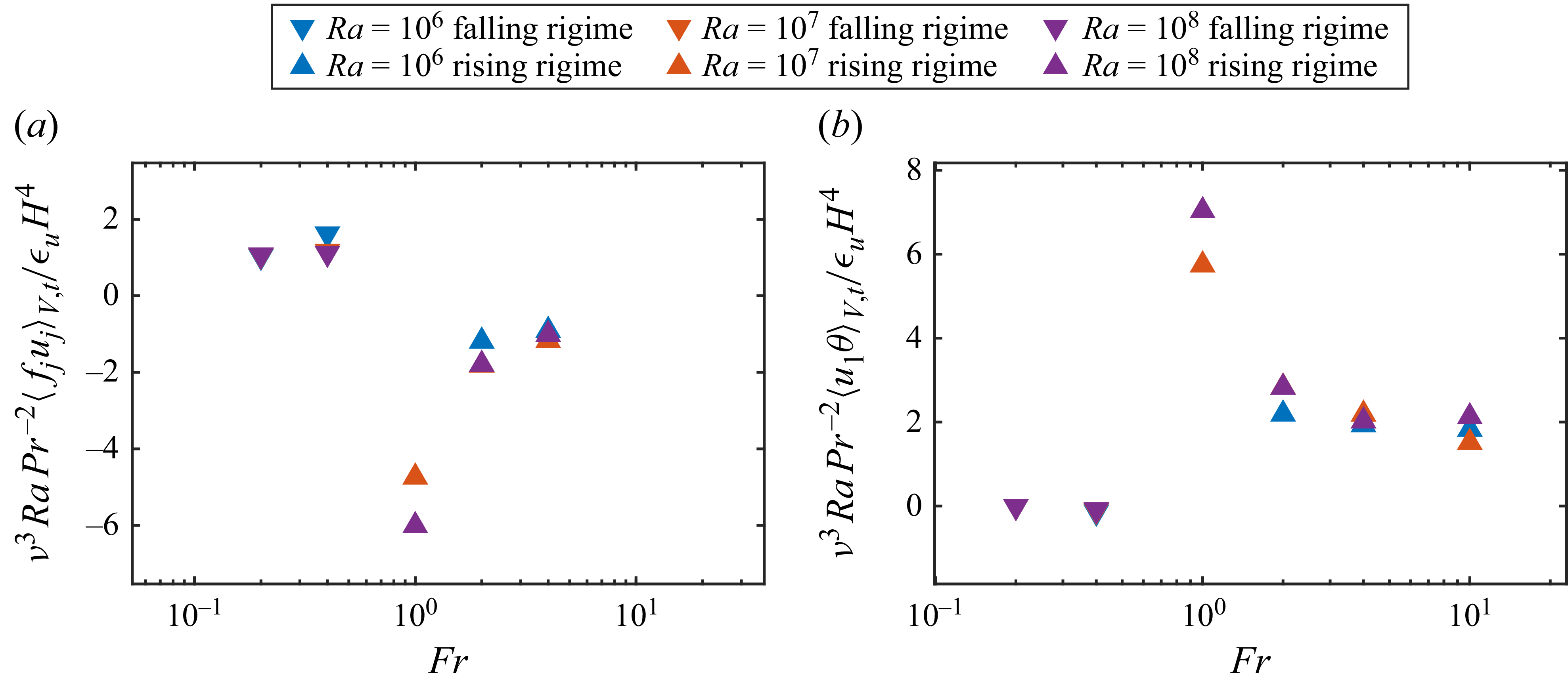
The two terms on the right-hand side of (3.7) are, respectively, the kinetic energy due to thermal buoyancy and the work done by the feedback force. The thermal energy dissipation rate in (3.8) is equal to the correction between the feedback heat flux and the local temperature. One important application of the above relations is to verify the adequacy of grid resolution (Stevens, Verzicco & Lohse Reference Stevens, Verzicco and Lohse2010). For all the simulations, the relative error between the two sides of the relations is always less than
 $5\,\%$
, indicating that the resolution is fine enough to capture the relevant small-scale structures.
Figure 8 shows the variations of the two terms on the right-hand side of (3.7) as a function of the Froude number
 $ \textit{Fr}$
. For cases with small
 $ \textit{Fr}$
, the descending particles drag the fluid downwards, resulting in negative vertical flow. In this regime, the particles do positive work on the fluid phase, while the buoyancy force does negative work. As
 $ \textit{Fr}$
increases, the settling velocity of the particles decreases, and correspondingly, the positive work done by particles also decreases. When
 $ \textit{Fr}$
exceeds a critical threshold, the fluid is driven upwards by buoyancy forces, simultaneously carrying the particles. In this regime, the buoyancy force performs positive work on the fluid, whereas the particles perform negative work and slow down the fluid motion. This inversion in energy exchange reflects a transition from a particle-driven falling regime to a buoyancy-driven rising regime.
(a) The particle-induced energy and (b) the thermal buoyancy-induced energy normalised by the total dissipation rate versus Froude number for different
 $ \textit{Ra}$
.

For the statistically steady state, the global balance of forces can also be established. By taking the temporal average of (2.6b ) and then the volume integral, one obtains
 \begin{eqnarray} &&\iint _{\partial V} \langle u_3 u_{\kern-1pt j} \rangle _t\, n_j\, \text{d}S/V - \iint _{\partial V} \langle p n_3 \rangle _t\, \text{d}S/V \nonumber \\[5pt]&&\quad = Ra^{-1/3}\,Pr^{2/3} \iint _{\partial V} \left\langle \frac {\partial u_3}{\partial x_j}\right\rangle _t n_j\, \text{d}S/V + \langle \theta \rangle _{V,t} + \langle f_3 \rangle _{V,t}. \end{eqnarray}
Here, we already used the non-divergence condition and the Gauss theorem. The periodic conditions in the
 $x_2$
- and
 $x_3$
-directions, and the no-slip condition at two walls, imply that the two surface integrals on the left-hand side vanish, and the first term on the right-hand side only has the contribution from the wall integral. Then (3.9) can be simplified to
 \begin{align} F_{shear} = Ra^{-1/3}\,Pr^{2/3}\left (\frac { \mathrm{d} \overline {u_3}}{\mathrm{d}x_1}\Bigg |_{x_1=0} - \frac { \mathrm{d} \overline {u_3}}{\mathrm{d} x_1}\Bigg |_{x_1=1}\right )= \langle \theta \rangle _{V,t} +\langle f_3 \rangle _{V,t}, \end{align}
which is nothing but the balance between the wall shear force, the buoyancy force, and the feedback force of particles for the fluid phase.
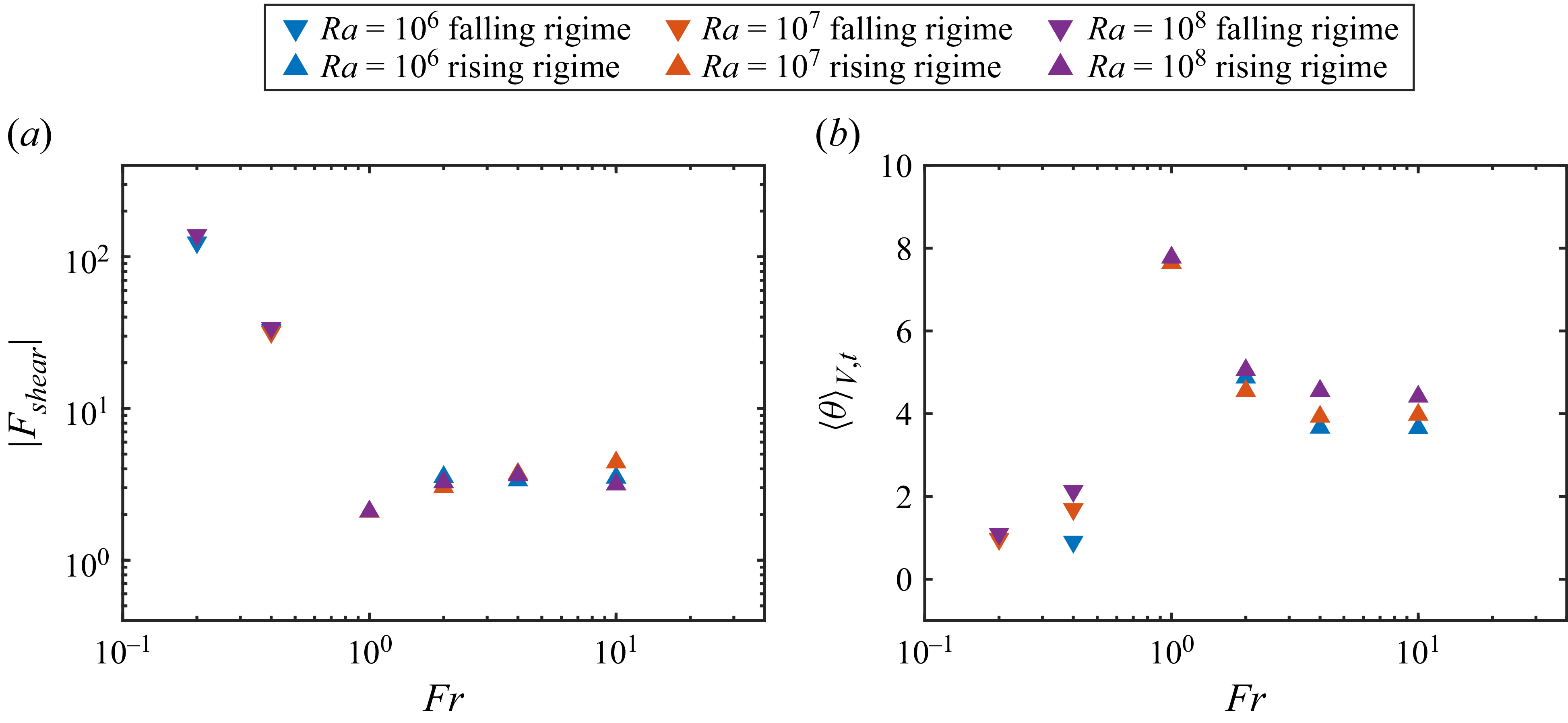
The variations of the magnitude of wall shear force
 $|F_{shear}|$
and the buoyancy force
 $\langle \theta \rangle _{V,t}$
are shown in figure 9. The wall shear force exhibits pronounced variation with
 $ \textit{Fr}$
. Generally, it decreases with
 $ \textit{Fr}$
in the falling regime, then increases with
 $ \textit{Fr}$
in the rising regime. As shown in figure 9(b), the buoyancy force exhibits a non-monotonic dependence on the Froude number, initially increasing and then decreasing. Moreover, it increases monotonically with Rayleigh number.
The variation of (a) wall shear force
 $F_{shear}$
and (b) buoyancy force
 $\langle \theta \rangle _V$
versus Froude number
 $ \textit{Fr}$
.

We now derive the scaling relations for the wall shear force and the mean temperature, which will be used to determine the critical parameters corresponding to the transition between the falling and rising regimes in the next subsection. In particular, we are seeking their scaling relations to the Rayleigh number, the Prandtl number and the bulk Reynolds number. By using the power-law scaling between
 $ \textit{Re}_\tau$
and
 $ \textit{Re}_b$
, the wall shear force should follow the scaling
 \begin{align} F_{shear}= 2 \tau _w = 2\, Ra^{-2/3}\,Pr^{4/3}\,Re_{\tau }^2 \sim \gamma\, Ra^{-2/3}\,Pr^{4/3}\, Re_b^{1.74}. \end{align}
By using the scaling law for the Nusselt number, one has
 \begin{align} \langle \theta \rangle _V = \frac {Ra^{1/3}\,Pr^{1/3} }{6 Nu} \sim Ra^{1/3}\, \textit{Pr}^{1/3}/ (\beta\, Re_b^{0.79} + 6). \end{align}
In figure 10, the scaling relations (3.11) and (3.12) are compared with the numerical results, and the agreement is good. The coefficients
 $\gamma$
and
 $\beta$
are determined through least squares fitting as
 $\gamma =0.073$
and
 $\beta =0.037$
.


3.3. The identification of the falling and rising regimes
As shown in figure 2, the rising and falling regimes exist in the simulated parameter space, and the critical Froude number divides these two regimes. To understand the transition mechanism, we first idealise the scene for the critical Froude number as the situation where the particles are uniformly distributed.
The instantaneous contours of temperature field and the particle distributions on (a–d) the mid vertical plane and (e–h) the mid horizontal plane with
 $ \textit{Ra}=10^7$
and different
 $ \textit{Fr}$
: (a,e)
 $ \textit{Fr}=0.2$
, (b,f)
 $ \textit{Fr}=0.4$
, (c,g)
 $ \textit{Fr}=1$
, (d,h)
 $ \textit{Fr}=10$
.

For the considered parameters in figure 2, the particle gravity and Stokes drag are dominant in the direction of gravity, and the Saffman lift force is neglected in the direction of gravity. It should be noted that we do not neglect the Saffman lift force. Only the component of Saffman lift force in the gravity direction is neglected in the following relation. The reason is that in our flow configuration, the dominant mean shear is
 $\partial \overline {u_3}/\partial x_1$
, which generates a wall-normal lift force according to the Saffman–Mei model, while the component in the gravity direction is relatively small. Then we can obtain the following approximate relation in the direction of gravity:
 \begin{align} \langle \mathrm{d}_t u_{3,p}\rangle _{p,t} =C_D\frac {\langle u_{3,f}-u_{3,p}\rangle _{p,t}}{St} - \frac {1}{Fr^2}. \end{align}
Here,
 $\langle {\cdot }\rangle _{p,t}$
stands for average over all particles and time. For the critical Froude number, the particle velocity in the direction of gravity is very small, namely
 $u_{3,p} \approx 0$
. The term
 $0.15\,Re_p^{0.678}$
is small relative to unity in the present parameters, as shown in figure 13 below. When the vertical velocity of the particles approaches zero, the flow is necessarily directed upwards, thereby exerting an upward Stokes drag on the particles to balance gravity. According to (2.12), the mean upward fluid velocity averaged over all particles can be estimated as
 $\langle u_{3,f}\rangle _{p,t} \sim \langle u_3\rangle _{V,t} \sim Ra^{-1/3}\, \textit{Pr}^{2/3}\, Re_b$
. Thus we can obtain the relation between the critical Froude number
 $ \textit{Fr}_{\textit{cr}}$
and the bulk Reynold
 $ \textit{Re}_{b,cr}$
in the transition state:
 \begin{align} \textit{Fr}_{\textit{cr}} = \sqrt {\frac {St\, Ra^{1/3}} {Pr^{2/3}\, Re_{b,cr}}}. \end{align}
In (3.10), the volume average of the vertical component of the particle feedback force
 $\langle f_3 \rangle _{V,t}$
is balanced by the wall shear force
 $F_{shear}$
and the buoyancy force
 $\langle \theta \rangle _{V,t}$
. Considering upward flow motion and
 $u_{3,p} \approx 0$
, the direction of
 $\langle \theta \rangle _{V,t}$
is opposite to that of the
 $\langle f_3 \rangle _{V,t}$
and
 $F_{shear}$
. Moreover,
 $\langle f_3 \rangle _{V,t}$
equals the Stokes drag acting on the particles. Consequently, we can derive the relation for the critical bulk Reynolds number
 $ \textit{Re}_{b,cr}$
:
 \begin{align} \textit{Ra}^{1/3} \textit{Pr}^{1/3}/ \big(\beta \textit{Re}_{b,\textit{cr}}^{0.79}+6 \big) -\varPhi _M \frac {Pr^{2/3} \textit{Re}_{b,\textit{cr}}}{\textit{St} \textit{Ra}^{1/3} } -\gamma \textit{Ra}^{-2/3} \textit{Pr}^{4/3} \textit{Re}_{b,\textit{cr}}^ {1.74} =0. \end{align}
By solving this equation, the bulk Reynolds number corresponding to the transition state can be obtained for different Rayleigh numbers. The critical Froude number can then be calculated accordingly using (3.14). As shown in figure 2, the predictions given by the above scaling law precisely identify the boundaries between the falling and rising regimes.
4. Preferential concentration and statistics of particles
We now turn to the spatial distribution and associated statistics of particles. The instantaneous temperature fields and particle distributions are shown in figure 11 for four cases with
 $ \textit{Ra}=10^7$
and different Froude numbers. The system features a non-uniform internal heat source arising from the moving particles, which releases heat into the fluid. In contrast, the walls act as sinks, extracting heat from the system. Thus the fluid temperature in the bulk is higher than that of the two plates. As the Froude number increases, the balance between internal heating and wall cooling shifts, leading to a rise in mean fluid temperatures initially, followed by a decrease. As seen in figures 11(e–h), the high-temperature region is asymmetric about the channel centreline. The reason is that the combined effect of Saffman lift force and turbophoretic transport can produce instantaneous asymmetric particle distribution in the wall-normal direction, as seen in figures 11(e–h), leading to asymmetric heat source and temperature field. It is worth noting that after averaging for a sufficiently long time, the particle distribution becomes left–right symmetric, as shown in figure 12.
For the case with the smallest Froude number,
 $ \textit{Fr}=0.2$
, the particle distribution is nearly uniform across the entire flow domain. Meanwhile, no significant accumulation of particles is observed near the walls. In contrast, it is observed that particles tend to accumulate near the walls in the cases with larger Froude numbers in the falling regime or the rising regime. For the cases in the rising regime, particles also tend to accumulate in the high-temperature region at the centre of the channel, and experience very strong non-uniform distribution in the wall-normal direction. We compute the particle volume fraction within the near-wall region (
 $x_1^+\lt 30$
)
 $\varPhi _{\textit{NW}}$
, and normalise it by the global mean particle volume fraction
 $\varPhi _{V}$
. This ratio
 $\varPhi _{\textit{NW}}/\varPhi _{V}$
quantitatively described the near-wall accumulation of the particles. The results, summarised in table 1, show that
 $\varPhi _{\textit{NW}}/\varPhi _V$
increases with
 $ \textit{Fr}$
separately in the falling and rising regimes, consistent with the distribution of particles shown in figure 11.
The p.d.f.s of wall-normal position of the particles with (a)
 $ \textit{Ra}=10^6$
, (b)
 $ \textit{Ra}=10^7$
and (c)
 $ \textit{Ra}=10^8$
.

In the following, we focus on the inhomogeneous distribution of particles along the wall-normal direction. The probability density function (p.d.f.) of the wall-normal location of particles
 $x_{1,p}$
is shown in figure 12 for different
 $ \textit{Ra}$
and
 $ \textit{Fr}$
. In the falling regime, a pronounced accumulation near the wall is observed for the case with
 $ \textit{Ra} = 10^7$
and
 $ \textit{Fr} = 0.4$
. As the Rayleigh number increases and the Froude number decreases, the accumulation of particles near the wall is suppressed. In the rising regime, particles accumulate near the wall under different Froude numbers and Rayleigh numbers, with the accumulation becoming more pronounced as the Froude number increases.
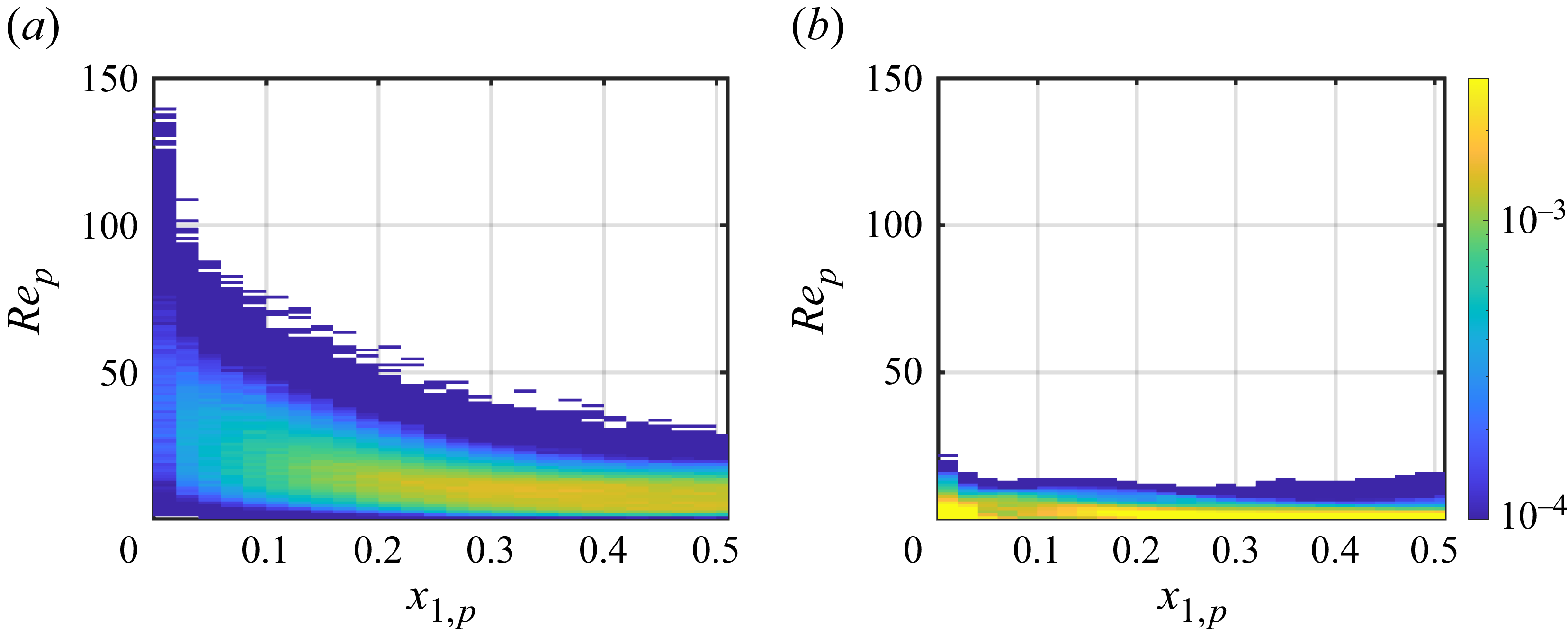
To quantitatively measure the possible slip velocity distribution, figure 13 plots the p.d.f. of the particle Reynold number for different Rayleigh numbers and Froude numbers. For the smallest Froude number,
 $ \textit{Fr}=0.2$
, the p.d.f. of the particle Reynolds number exhibits a higher magnitude in the range of larger
 $ \textit{Re}_p$
. As the Froude number increases, the peak of the p.d.f. shifts towards smaller
 $ \textit{Re}_p$
. For the cases with larger Froude number, the p.d.f. exhibits a dominant concentration below
 $1$
, and a suppressed high-
 $ \textit{Re}_p$
tail, indicating less frequent strong slip events compared to small Froude numbers.
This trend can be interpreted from the vertical momentum exchange between particles and fluid. As seen in (2.7), the slip velocity directly determines the volume-averaged vertical feedback force
 $\langle f_3 \rangle _{V,t}$
. According to (3.10),
 $\langle f_3\rangle _{V,t}$
is balanced by the wall-shear force
 $F_{{shear}}$
and the buoyancy term
 $\langle \theta \rangle _V$
. In the falling regime, considering downward flow motion, the direction of
 $\langle f_3 \rangle _{V,t}$
is opposite to that of
 $\langle \theta \rangle _{V,t}$
and
 $F_{shear}$
. As shown in figure 9, the wall-shear stress decreases with
 $ \textit{Fr}$
and is obviously larger than
 $\langle \theta \rangle _{V,t}$
. Thus when
 $ \textit{Fr}$
increases,
 $\langle f_3 \rangle _{V,t}$
decreases, indicating a trend towards reduced slip velocity.
In contrast, in the rising regime, considering the upward flow motion, the direction of
 $\langle \theta \rangle _{V,t}$
is opposite to that of
 $\langle f_3 \rangle _{V,t}$
and
 $F_{shear}$
. As seen in figure 9,
 $\langle \theta \rangle _{V,t}$
and
 $F_{shear}$
are of comparable magnitude, The mutual cancellation of their effects leads to a relatively small
 $\langle f_3 \rangle _{V,t}$
, indicating small particle slip velocity.
The p.d.f.s of particle Reynolds numbers with (a)
 $ \textit{Ra}=10^6$
, (b)
 $ \textit{Ra}=10^7$
and (c)
 $ \textit{Ra}=10^8$
.

The correction between the wall-normal location of particles and the slip velocity is shown in figure 14. For the case with
 $ \textit{Ra}=10^7$
and
 $ \textit{Fr}=0.2$
in the falling regime, there is a clear trend that particles near the wall are accompanied by higher particle Reynolds numbers. The peak of joint p.d.f. is near the centre of the channel, with smaller
 $ \textit{Re}_p$
. This indicates that most particles accumulate near the centre of the channel with relatively low slip velocities. In contrast, for the cases with
 $ \textit{Ra}=10^7$
and
 $ \textit{Fr}=10$
in the rising regimes, the slip velocity is relatively small at different wall-normal positions.
Joint relative probability for the wall-normal location of particles and particle Reynolds number with
 $ \textit{Ra}=10^7$
and different Froude numbers: (a)
 $ \textit{Fr}=0.2$
, (b)
 $ \textit{Fr}=10$
.

Considering the strong near-wall mean shear
 $\text{d} \overline {u_3}/\text{d} x_1$
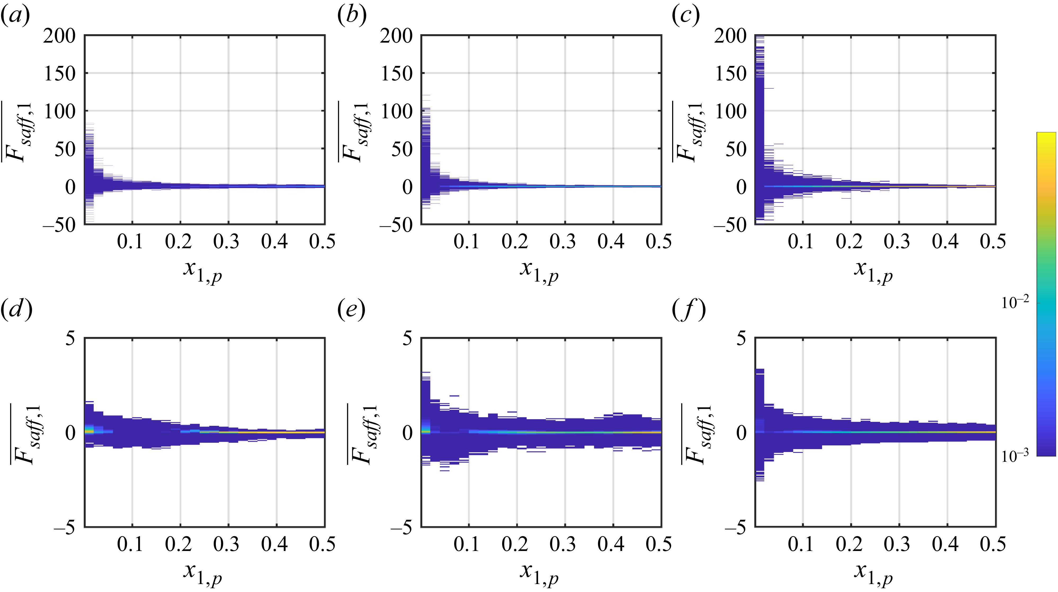
shown in figure 3, the wall-normal component of the Saffman force is expected to dominate the streamwise and spanwise components according to the Saffman model. We therefore investigate the wall-normal lift force as shown in figure 15. The Saffman force becomes significant near the wall especially in the falling regime, due to the large slip velocities between the two phases as shown in figure 14. Meanwhile, the magnitude of the Saffman force increases as the Rayleigh number
 $ \textit{Ra}$
increases and the Froude number
 $ \textit{Fr}$
decreases.
Joint relative probability for the wall-normal location of particles and wall-normal lift force for different
 $ \textit{Ra}$
and
 $ \textit{Fr}$
: (a,d)
 $ \textit{Ra}=10^6$
, (b,e)
 $ \textit{Ra}=10^7$
and (c,f)
 $ \textit{Ra}=10^8$
, with (a–c)
 $ \textit{Fr}=0.2$
and (d–f)
 $ \textit{Fr}=10$
.

The particle distribution along the wall-normal direction is influenced by turbophoresis and the Saffman lift force. We first analyse the situation in the falling regime. For the case with
 $ \textit{Ra} = 10^6$
and
 $ \textit{Fr} = 0.2$
, most particles experience the positive Saffman force near the left-hand wall and the negative force near the right-hand wall as shown in figure 15, effectively driving particles away from the near-wall region and towards the bulk flow. Thus the Saffman lift force can significantly reduce the strength of turbophoresis and the near-wall accumulation of particles as shown in figure 12, consistent with previous studies (Li, Wang & Zheng Reference Li, Wang and Zheng2024; Ruan & Xiao Reference Ruan and Xiao2024). The mean wall-normal component of the Saffman force averaged over the near-wall region (
 $x_1^+\lt 30$
) is shown in table 1. As
 $ \textit{Fr}$
increases, the Saffman lift force decreases, which in turn enhances particle accumulation near the wall region.
Then we turn to the rising regime. Figures 15(d–f) and table 1 show that the Saffman force is negligible, and turbophoresis dominates the wall-normal distribution. Reeks (Reference Reeks1983) has proven that the turbophoretic drift is proportional to the wall-normal derivative of the standard deviation of the wall-normal velocity for fixed Stokes number. As can be seen from figure 4(b), the derivative of the standard deviation of the wall-normal velocity increases as the Froude number increases from 1 to 10. Hence particles in the cases with small Froude numbers are subjected to a smaller turbophoretic drift, leading to a reduced wall accumulation, as confirmed in figure 12.
5. Conclusion
We have conducted a detailed numerical investigation of vertical thermal channel flow driven by heat-releasing particles. The particles absorb energy from an external source, and release it into the surrounding fluid, generating localised buoyancy forces that drive upward motions. Meanwhile, under the influence of gravity, the particles tend to settle downwards. The competition between buoyancy-induced upward driving and gravitational settling governs the overall flow regime and particle transport in the system. The silicon carbide particles suspended in air are considered, and the Stokes number is fixed at
 $ \textit{St} = 1$
. Three Rayleigh numbers,
 $ \textit{Ra} = 10^6$
,
 $10^7$
and
 $10^8$
, are examined, with several Froude numbers, ranging from
 $0.2$
to
 $10$
for each
 $ \textit{Ra}$
.
Within the parameter range explored here, the mean vertical velocity undergoes a gradual reversal across the domain with increasing
 $ \textit{Fr}$
, reflecting the interplay between buoyancy-driven rising and gravitational settling. The statistically steady state of the flow is horizontally symmetric. The friction Reynolds number and the Nusselt number exhibit monotonic dependence on the bulk Reynolds number, following power-law scalings with the exponents close to those obtained in the single-phase channel flow. The scaling laws are then used to explain the regime transition between the falling and rising regimes at intermediate Froude numbers.
The near-wall accumulation of particles is observed across a range of
 $ \textit{Fr}$
and
 $ \textit{Ra}$
, which is controlled by turbophoresis and the Saffman lift force. The Saffman lift force can reduce the influence of the turbophoresis. In the falling regime, as
 $ \textit{Fr}$
increases, the Saffman lift force decreases and enhances the particle accumulation near the wall. In the rising regime, as
 $ \textit{Fr}$
increases, the Saffman lift force is negligible, and larger turbophoretic drift leads to an enhanced near-wall accumulation.
A central finding is the identification of two distinct regimes of motion of the particles and fluid: the falling regime and the rising regime, separated by a critical Froude number
 $ \textit{Fr}_{\textit{cr}}$
. This threshold corresponds to a balance between particle gravity and buoyant acceleration, where the mean vertical velocity of the particles vanishes. The scaling analysis is consistent with the numerical results. The transition is also explained through an energy budget analysis, showing a reversal in interphase energy exchange, from the particle-driven state to the buoyancy-driven state, as
 $ \textit{Fr}$
increases.
This study opens up several interesting possibilities for future research. For instance, the radiation–particle interactions may be important in the present volume fraction. The radiative absorption and scattering process can be considered. The effects of particles properties, such as particle density and heat capacity, on the flow behaviour can be considered. These are the subjects of our ongoing research.
Funding
This work is financially supported by the National Natural Science Foundation of China under grant nos 12402252 and 52441501. Y.Y. acknowledges support from the NSFC Young Scientists Fund (A) under grant no. 12525209 and the NSFC Excellence Research Group Programme for ‘Multiscale problems in nonlinear mechanics’ under grant no. 12588201. This work is also funded by the Science and Technology Project of Hebei Education Department under grant no. BJK2024166.
Declaration of interests
The authors report no conflict of interest.
Appendix A. Numerical details
Summary of the simulated cases. Columns from left to right are the Rayleigh number, the Froude number, the resolutions in the wall-normal, spanwise and vertical directions, the bulk Reynolds number, the friction Reynolds number, the Nusselt number, the volume-average of temperature, the shear force, the ratio
 $\varPhi _{\textit{NW}}/\varPhi _{V}$
, the mean wall-normal component of the Saffman force in the near-wall region
 $\langle F_{\mathit{saff},1} \rangle _{x_1^+\lt 30,t}$
, respectively. For all cases,
 $ \textit{Pr}=0.7$
,
 $ \textit{St}=1$
,
 $\varPhi _V=2.3 \times 10^{-3}$
,
 $\rho _p/\rho _0=2469$
,
 $\varPhi _M=5.67$
and
 $c_p/c_{\kern-1pt f}=1.15$
. Cases marked with an asterisk represent those close to the regime transition.