Competition between Specialized Candidates

STEFAN KRASA; MATTIAS POLBORN

doi:10.1017/S0003055410000468

Competition between Specialized Candidates

Published online by Cambridge University Press: 08 December 2010

STEFAN KRASA and

MATTIAS POLBORN

Show author details

STEFAN KRASA*: Affiliation:
University of Illinois Urbana–Champaign
MATTIAS POLBORN*: Affiliation:
University of Illinois Urbana–Champaign
*: Stefan Krasa is Professor, Department of Economics, University of Illinois at Urbana–Champaign, 1407 W. Gregory Drive, Urbana, IL 61801 (skrasa@uiuc.edu).
Mattias Polborn is Associate Professor, Department of Economics and Department of Political Science, University of Illinois at Urbana–Champaign, 1407 W. Gregory Drive, Urbana, IL 61801 (polborn@uiuc.edu).

Article contents

Abstract
CAUSES AND CONSEQUENCES OF HETEROGENEOUS CANDIDATE ABILITIES
RELATED LITERATURE
MODEL
RESULTS
EXTENSIONS
CONCLUSION
Footnotes
References

Rights & Permissions

Abstract

Opposing candidates for a political office often differ in their professional backgrounds and previous political experience, leading to both real and perceived differences in political capabilities. We analyze a formal model in which candidates with different productivities in two policy areas compete for voters by choosing how much money or effort they would allocate to each area if elected. The model has a unique equilibrium that differs substantially from the standard median voter model. Although candidates compete for the support of a moderate voter type, this cutoff voter differs from the expected median voter. Moreover, no voter type except the cutoff voter is indifferent between the candidates in equilibrium. The model also predicts that candidates respond to changes in the preferences of voters in a very rigid way. From a welfare perspective, candidates are “excessively moderate”: almost certainly, a majority of voters would prefer that the winning candidate focus more on his or her strength.

Information

Type: Research Article
Information: American Political Science Review , Volume 104 , Issue 4 , November 2010, pp. 745 - 765
DOI: https://doi.org/10.1017/S0003055410000468 [Opens in a new window]
Copyright: Copyright © American Political Science Association 2010

In his seminal work “An Economic Theory of Democracy,” Anthony Downs (Reference Downs1957) develops a model of two-party electoral competition. In this framework, candidates propose identical, or at least similar, policies because they have to attract the support of the median voter to win, and voters do not perceive significant differences among candidates as the electoral campaign gravitates toward the median voter.

An alternative view of electoral competition postulates that candidates emphasize policy issues that assert their strengths (Budge Reference Budge and Riker1993; Budge and Farlie Reference Budge and Farlie1983; Petrocik Reference Petrocik1996; Riker Reference Riker and Riker1993, Reference Riker1996). The underlying intuition behind this view is that, because electoral candidates differ in their personal backgrounds, professional expertise, and policy reputations, the electorate perceives them as having different strengths and weaknesses in certain policy areas. For example, Republicans are often considered more competent on security matters, whereas Democrats are perceived as more competent on education or the environment.

Despite the empirical and substantive appeal of electoral competition as a contest between heterogeneous candidates with varying policy competencies, a rigorous theoretical analysis is missing. We therefore develop a game-theoretic model of electoral competition in which two candidates differ in their abilities in two distinct policy areas (e.g., security, education). The candidates are uncertain about the voters' preferences when they propose how to allocate a fixed budget between the two policies. The resource allocation, together with the winner's policy ability, determines the amount of the policy area-specific public goods provided to the voters. Voters prefer a higher output in each policy area, but they differ in how important each good is for them. This model shows that when candidates have heterogeneous abilities, the nature of electoral competition is substantially different from that in the Downsian model.

Our analysis yields several important implications for understanding the nature and welfare effects of political competition that also differ from the insights of the standard Downsian model. First, the candidates' platform policies usually diverge in equilibrium. Candidates may either choose to stress and exploit their respective strong suits by proposing to spend more money on that policy area than their opponent, or they may partially compensate for their respective deficiency by proposing to spend more money on their weak policy area. This result speaks to an empirical literature on electoral agenda strategy. Some studies suggest that that candidates campaign on issues that play to their strengths while avoiding issues that either accent the opposition's strengths or highlight their own weaknesses, a strategy that William Riker labeled the “dominance principle.” Other studies suggest that candidates sometimes engage in issue trespassing as they campaign in their opponent's issue territories. Our analysis provides precise conditions, depending on the specifics of the voters' utility functions, when we should observe issue divergence or issue trespassing at work.

Second, the analysis shows that candidates' equilibrium platforms display a strong rigidity when voters' perceptions of the importance of electoral issues change. That is, candidates are stuck pursuing policies focusing on their “strong” issues, even if the voters' priorities shift, because they cannot successfully imitate their opponent. This result helps us understand why a party can sustain dominance over the opposition party for an extended period of time. For example, it is generally acknowledged that the Democrats were the dominant political party from 1932 to 1968, whereas the Republican Party struggled to restructure its political message. Our model suggests that if Republicans cannot successfully imitate the Democrats' policy position, then sticking with their old platform and hoping for a reversal of the preference shift is their best strategy (from an electoral perspective) in the short to medium run. However, when the preference shift persists, a party would have to “reinvent” itself and change its perceived policy strengths and weaknesses.

Third, our analysis suggests that the voting majority would prefer that the winning party further accentuate the policy difference between itself and the losing party rather than trend toward the middle. The reason for this is that in our framework, the two candidates cater to a marginal “cutoff” voter type who is indifferent between the candidates; all voters to the left of the cutoff voter strictly prefer the Democrat, whereas all voters to the right of the cutoff strictly prefer the Republican. A candidate wins if and only if a strict majority of the electorate is on his or her side of the cutoff voter, and as a result that majority would be better pleased if the winner implemented a more partisan policy in office than promised in the policy platform. Thus, supermajoritarian institutions that foster bipartisanship and moderation, but prevent electees from implementing their policies may be detrimental to society. This result stands in stark contrast with the point of view of a large segment of “moderate” political pundits that moderation and bipartisanship are inherently beneficial for society, a school of thought sometimes called “Broderism” (after David Broder of the Washington Post).

The article proceeds as follows. We first discuss the causes of differences in candidate ability and describe our results, followed by a section in which we relate our article to previous literature. This is followed by a description of the model and the analysis of the equilibrium, which is done for the most part using graphics (generalized theorems and proofs appear in the Appendix). We also discuss the robustness of the model to several extensions before concluding.

CAUSES AND CONSEQUENCES OF HETEROGENEOUS CANDIDATE ABILITIES

Policy Areas and Differences between Candidates

The key departure of our model from previous literature is that we assume that candidates have differential abilities in the different policy areas. To this end, our model focuses on policy areas that stokes (Reference Stokes1963) calls “valence issues.” That is, voters in our model agree that a higher output in both public goods (a low crime rate, the quality of schooling, etc.) is desirable, but they differ on which trade-offs to make between these different political goals. To focus our model on the effect of heterogeneous candidate abilities on electoral competition, we disregard what Stokes calls “position issues”—policy issues such as abortion, gay marriage, or gun control, where voters disagree over the desired outcome and a candidate's implementation ability is of lesser importance.

There are several reasons why candidates (or parties) have different policy abilities. First, individual candidates already have a background (education, experience, personal interests) when they enter politics, and this background may focus their interests on certain policy issues rather than others. When business leaders run for elected office, they usually highlight their management experience as a reason to expect competent management of government from them. Likewise, candidates with military backgrounds often leverage their experience on military and foreign affairs issues and focus their policy proposals on this area.

Second, once in office, individuals may choose to work on those issues in which they are more capable, self-selection that further strengthens whatever initial competency the candidate brings to those specific policy issues. For example, it is plausible that Franklin Delano Roosevelt, after having started the New Deal program in his first term, was considered more competent in managing a more active government involvement in the economy than any Republican challenger. Similarly, George W. Bush successfully leveraged his perceived experience in fighting the “war on terror” in his 2004 reelection campaign.

Third, citizens sort themselves into parties based on their backgrounds and preferences, and so individuals who become candidates are first citizens with certain policy preferences. If an individual has a stronger than average preference for national defense, for example, then it is natural that he or she will be especially interested in foreign relations or defense technology. Over time, competency on defense-related matters will increase, while education-related competency will be weaker than that of an individual who cares more about education. Moreover, it is not only natural that these individuals will join parties composed of individuals with preferences similar to their own, but there are also career incentives for aspiring politicians to self-select into the party that most appreciates their specific competencies, as say, national defense is more appreciated by the members and primary voters of the Republican Party.

Fourth, and complementary to the third explanation, parties can be seen as networks whose members cooperate in providing government services. If, for whatever reasons, one party has attracted many individuals with specific knowledge about one policy area, then an elected candidate from this party can draw on this network both to provide specific new ideas and to recruit key personnel for government positions. In contrast, if the competitor from the other party is elected, then he or she would not be able to draw on these network resources, limiting the ability to implement policy in this field. In this way, the ideological predisposition of party members may influence what policies their candidate is capable of offering, and, in addition, which policy (i.e., budget allocation) their candidate will choose.

In the standard model, competency is sometimes incorporated as an additive “valence” component. However, because valence enters voters' utility functions in a way that is separable from which policy is implemented, it does not capture the notion of issue-specific ability, which lies at the core of our model. For example, military experience is electorally more valuable for a candidate when international conflict is a serious concern for voters than when they are mostly concerned with economic issues.

Heterogeneous Candidates Competing for Voters

In our model, the two office-motivated candidates have unequal abilities in two distinct policy areas such as education and law enforcement, or domestic and foreign policy. During the campaign, each candidate proposes allocations for a fixed total amount of money (or effort) across the policy areas. Resources spent in each policy area, together with the winner's ability, translate into the amount of public goods provided in each policy area. Voters prefer a higher output in both areas (e.g., more security and higher-quality education), but their priorities run along a continuum between the two goods, ranging from those who almost only care about good 0 to those who care almost exclusively about good 1. In a (Nash) equilibrium, each candidate's policy maximizes his or her probability of victory in the election, given the opponent's proposed policy.

If both candidates have identical abilities, as in the Downsian model, then both propose a policy that maximizes the utility of the median median voter. (Candidates in our model are uncertain about the exact priorities of the median voter so that they have to cater to the “median median” voter, that is, the median realization of the median voter). Because both candidates propose the same policy, all voters are indifferent between the candidates.

However, if candidates have different strengths, the nature of electoral competition changes substantially. Candidates have a natural respective target audience, in the sense that they have an advantage in appealing to these voters. Assume that the candidate who has a productivity advantage in the production of good 0 ends up producing more of good 0 than his or her competitor, and vice versa for good 1 (our results show that such “no overcompensation” is in fact a property of equilibrium). In this case, voters who care primarily about good 0 vote for candidate 0, and those voters who care primarily about good 1 vote for candidate 1.

Between the extremes is a moderate cutoff voter, characterized by some intermediate intensity with which he or she cares about the provision of the two goods. The identity of this cutoff voter is independent of the voter preference distribution; that is, the cutoff voter is not the median voter. More specifically, this cutoff voter is indifferent between candidates if both candidates propose the cutoff voter's optimal budget allocation, given that candidate j is elected. We show that, in equilibrium, both candidates compete fiercely for the support of this cutoff voter and indeed choose the optimal budget allocation for the cutoff voter t. All voter types below the cutoff voter t strictly prefer candidate 0, whereas those above t strictly prefer candidate 1. Which candidate wins the election depends on whether the realized median voterFootnote ¹ in this society is a type below t (then candidate 0 wins), or above t (then candidate 1 wins). Thus, the realized median voter in our model is still decisive for who wins the election. However, the type whose utility is maximized is the cutoff voter t.

Although the cutoff voter is indifferent in equilibrium, all other voters strictly prefer one of the candidates. Specifically, those voters who have a stronger preference than the cutoff voter for the “democratic” good strictly prefer the Democratic Party, whereas the remaining voters strictly prefer the Republican Party. Thus, even though candidates can, in principle, compensate for competency differentials by spending more money on their “weak” good, the initial asymmetry is never wiped out completely and generates captive support groups for the two parties. This result occurs without appealing to some exogenous “partisan” preference—voters in our model do not care about party labels, but the equilibrium platform of each candidate appeals more to a particular set of voters.

Equilibrium Properties and Comparison to the Literature

The equilibrium has several interesting features that we now compare to equilibrium properties in other existing models.

Policy Divergence. In our model, there is always policy divergence in terms of policy outcomes (i.e., the bundle of goods that each candidate would provide). However, the actual policy “output” may be difficult to measure empirically. For example, the “level of national security” provided by a candidate would be difficult to measure objectively by an outside observer, but spending on national security–related items is clearly defined. In addition, the model features policy divergence in terms of budget allocation, and this divergence can be easier to measure empirically.Footnote ²

The platform choice of candidates for political office is one of the major areas of interest in formal models of politics. There is an extensive literature on the topic of policy convergence or divergence in one-dimensional models (or models with one policy dimension and one valence dimension).Footnote ³

Policy divergence can be obtained in the Downsian framework by assuming that candidates are policy motivated (Calvert Reference Calvert1985; Groseclose Reference Groseclose2001; Martinelli Reference Martinelli2001; Roemer Reference Roemer1994; Wittman Reference Wittman1983). In this type of model, policy divergence reduces a candidate's winning probability, but increases his or her utility in case of a victory. This trade-off is affected by a number of exogenous factors. First, better information about the median voter's preferences translates into less policy divergence. Second, the arrival of new information (e.g., opinion polls conducted during the campaign) should induce candidates to adjust their positions. Third, policy divergence should be less pronounced in races for more prestigious, higher-paying offices. In contrast, in our model, candidates choose divergent policies in order to maximize their respective winning probabilities, and policy moderation would decrease rather than increase a candidate's probability of winning. Simply put, none of the factors detailed previously would change the candidates' equilibrium positions.

Apart from being empirically distinguishable from divergence in the standard framework, the interpretation of policy divergence in our model also leads to new substantive insights. The median voter model has become the standard framework through which scholars typically study electoral competition, and has also deeply influenced how journalists and practitioners think about political competition. For example, Suellentrop (Reference Suellentrop2004) writes two days before the 2004 elections:

The secret of Bill Clinton's campaigns and of George W. Bush's election in 2000 was the much-maligned politics of small differences: Find the smallest possible majority that gets you to the White House. In political science, something called the median voter theorem dictates that in a two-party system, both parties will rush to the center looking for that lone voter—the median voter—who has 50.1 percent of the public to the right (or left) of him. Win that person's vote, and you've won the election.

In contrast, Suellentrop anticipated that Bush had made a fatal mistake in the 2004 election by not converging enough toward his opponent's position: “Bush's campaign—and his presidency—have appealed almost entirely to the base of the Republican Party. . . . Rove has tried to use the Bush campaign to disprove the politics of the median voter.” Like in the median voter model, candidates in our model have to attract the support of the realized median voter to win. However, the best way for a candidate to maximize his or her winning probability is not by trying to appeal to the expected median voter, but rather to choose a platform that uses the candidate's strength to maximize the set of voters who prefer him or her over his or her opponent. Optimal platforms in our model generate a strict preference from a candidate's “natural” supporters, those voters who care primarily about a candidate's strong policy area.

Competition for Cutoff Voters' Support. Just as in the Downsian model, there exists one voter type in our model whose utility both candidates maximize. However, in the Downsian model, this type is always the median voter (or the median median, if the voter preference distribution is uncertain). In contrast, in our model, the location of this voter depends solely on the differential abilities of the candidates and will, in general, not coincide with the median. Furthermore, unlike in the Downsian model, our candidates offer different policies and only the cutoff voter is indifferent, whereas all other voters have a strict preference. Thus, our model can reconcile the notion that candidates compete fiercely for the support of some moderate voters with the observation that, in most major elections, many voters feel passionately that there is a significant difference between candidates.

Distribution Independence, Winning Probabilities, and Rigidity. In the standard model, the positions of the candidates' platforms are determined by the expected position of the median voter and thus depend decisively on the distribution of voter preferences. Likewise, in the two-candidate equilibrium of the citizen–candidate model (see Besley and Coate Reference Besley and Coate1997 and Osborne and Slivinski Reference Osborne and Slivinski1996), the two candidates locate at the same distance on opposite sides of the median voter's ideal point. Thus, although there is equilibrium policy divergence and most voters have strict preferences for one of the candidates, the equilibrium platforms shift with the distribution of voter preferences.

Our model substantially differs in this regard. In our framework, the equilibrium platforms of candidates depend exclusively on candidate skills and properties of the utility function, but not on the voter type distribution. For example, if there is improved information about the likely voter type distribution because of a new opinion poll, then candidates in our model would not want to adjust their platforms. This rigidity of candidates also implies that changes of the likely voter preference distribution would affect the candidates' winning probabilities. Note also that the candidates' winning probabilities are different in our model unless the cutoff voter type coincides with the median median, a very special case that is unlikely to arise in reality. In contrast, in the Downsian and the citizen candidate models, both candidates win with probability 1/2 for all distributions of voter preference types.

The fact that moderation (relative to the equilibrium platforms) is a bad electoral strategy for candidates does not necessarily imply that it would be unpopular. It is possible that a majority of the electorate would “sincerely” prefer that the weaker candidate's position becomes more moderate.Footnote ⁴ However, these voters for whom moderation is popular have a strict preference for the opponent that the weaker candidate cannot overcome. In equilibrium, candidates focus on voters who are close to indifferent between the candidates, and the preferences of these “swing voters” (rather than the majority's) are decisive for the positions that candidates take. If policy divergence arises in a Downsian world, the losing candidate always regrets his or her position choice: he or she could have done better (and maybe won the election) with a different policy position. In contrast, if a candidate loses in our model because too many voters cared strongly about the good in which his or her opponent had an advantage, then there is really nothing that could have changed the election outcome.

Given the previous point, our model implies that the only successful strategy for a losing party is a long-term strategy of redefining its policy strength. For example, consider the Labour Party in the UK. The Labour Party lost power in 1979, plausibly due to a fundamental and persistent change in the preference distribution of voters (say, more emphasis on economic growth relative to social justice). In the interpretation of our model, the party is initially stuck with its previously successful leaders who are specialists in social justice. During this time, we would expect party platforms to change very little, and the party just to hope that the voters will return to their previous preferences. If this does not happen, then popular support for the party is correspondingly reduced. Over the longer term, however, the Labour Party in our example fostered the development of new leaders who specialized more in being able to deliver on economic growth (while being weaker on social justice). Only when these new leaders were in place could a corresponding adjustment of the party platform be implemented that eventually brought the party on track for a return to power.

Our result on electoral rigidity corresponds very well to the argument of Petrocik (Reference Petrocik1996, 829) that “A Democrat's promise to attack crime by hiring more police, building more prisons and punishing with longer sentences would too easily be trumped by greater GOP enthusiasm for such solutions. . . . Candidates respond thus because . . . to do otherwise would advantage their opponent.” In other words, the candidate weak in a particular policy area cannot benefit by simply copying the platform of the strong candidate in this area.

Valence vs. Position Issues. Although we emphasized the differences between our model and the Downsian model when comparing their results, we do not want to frame our model as an exclusive alternative, but rather as a complement to the standard model because they apply to different types of policy issues. Our model applies for valence issues—settings where voters agree that more output is desirable, even though they disagree about trade-offs, and where candidates may have differentiated abilities in supplying these goods. In contrast, the Downsian model with identical candidates is a more useful framework for thinking about position issues such as gun control or gay marriage in which differences in implementation ability are more or less immaterial. This creates a useful testable implication. Shifts of the voter preference distribution in valence issues should affect candidates' positions much less than shifts of the voter distribution in position issues.

Welfare Implications. Our model is important for our understanding and interpretation of the results of electoral competition. In the standard model, policy convergence to the policy preferred by the median appears efficient in the sense that there is no other policy that a candidate could propose that would increase the utility of a majority of voters. Moreover, to the extent that policy divergence arises in the standard framework (e.g., in the citizen–candidate model), moderation would be beneficial in the sense that, if the winning candidate implements a policy that departs from his or her election platform in the direction of his or her opponent's platform, a majority of the electorate would benefit. This result has been influential in shaping the point of view of a large segment of “moderate” political pundits that moderation and bipartisanship is inherently beneficial for society. This school of thought is (sometimes satirically) called Broderism and defined by the Urban Dictionary as “the worship of bipartisanship for its own sake.”Footnote ⁵

In contrast, in our model, a majority of voters would approve if the winning candidate further accentuated the policy differences to the beaten competitor that were the reason for the candidate's victory in the first place. For example, suppose that the Democrat wins the election. This happens if and only if a majority of voters have “more liberal” preferences than those of the cutoff voter (i.e., care more for those goods that the Democrat has an advantage supplying). In other words, in his or her attempt to maximize the set of voter distributions for which the candidate wins the election, the Democrat caters during the election campaign to a cutoff type with more conservative preferences than those of a strict majority of the electorate. Thus, a majority of the electorate would be better off ex-post if the Democrat provided a more partisan policy than promised in the election platform. Of course, by the same argument, when the Republican wins the election, a majority of the electorate prefers a more partisan Republican policy than the cutoff voter.

Clearly, our model also has important implications for the interpretation of supermajoritarian institutions that encourage bipartisanship and “moderation.” Suppose, for example, that the filibuster rule in the U.S. Senate prevents Democrats from implementing the strong health insurance reform that they promised during the election campaign of 2008 and forces them to accept a more watered-down version that is palatable to the most conservative Democrats and/or the most liberal Republicans. Interpreted in a standard framework, such enforced moderation is plausibly beneficial because the preferences of the median voter are likely to be somewhere between the Democratic and the Republican election platforms. In contrast, in our framework, the reason why Democrats won the elections is that a majority of the electorate favored their platform and would be happy with an even more radical reform. Any institutional constraint that prevents Democrats from implementing their election platform would be detrimental in our framework.Footnote ⁶

RELATED LITERATURE

Our model starts from the premise that candidates are not only exogenously differentiated with respect to some characteristic (specifically, their public good production productivity), but can also choose a policy platform (specifically, the budget allocation) in order to compete for voter support. Krasa and Polborn (Reference Krasa and Polborn2009a) analyze general models of political competition with this feature and characterize a class of uniform candidate ranking (UCR) voter preferences that generically lead to policy convergence, even if candidates have differentiated characteristics. Although almost all models in the existing literature have UCR preferences, the present model with differentiated production possibilities violates UCR. This is the fundamental reason for equilibrium divergence in this article.Footnote ⁷

There are two classes of models in the existing literature that not only analyze settings in which candidates are exogenously differentiated, but can also choose policies: valence models and probabilistic voting models. In valence models (e.g., Ansolabehere and Snyder Reference Ansolabehere and Snyder2000; Aragones and Palfrey Reference Aragones and Palfrey2002; Groseclose Reference Groseclose2001, the candidates' fixed characteristics are quality parameters that enter additively in all voters' utility functions. Therefore, valence does not change a voter's ideal policy, in contrast to our model in which voter preferences over fixed characteristics and policies interact in a way that a voter's ideal budget allocation in general depends on the identity of the candidate.

In probabilistic voting models (Coughlin Reference Coughlin1992; Lindbeck and Weibull Reference Lindbeck and Weibull1987, Reference Lindbeck and Weibull1993) voter (groups) differ in their preferences over policy chosen by the candidates, and individual voters, in addition, experience an “ideological shock” for one of the two candidates that influences their utility and voting behavior. The ideology shock can be interpreted as arising from voter preferences over some candidate characteristics or positions that are exogenously fixed.Footnote ⁸ In equilibrium, there is policy convergence: both candidates choose a platform that maximizes a weighted sum of the utilities of all voters, where the weights reflect how “movable” certain voter groups are.

The probabilistic voting model closest to our article is Dixit and Londregan (Reference Dixit and Londregan1996) (henceforth DL). Two candidates differ in how efficient they are in transferring money to different interest groups and choose which transfer promises to make. In equilibrium, they choose to give higher transfers to the groups for which they have a higher transfer expertise. DL's main focus is on the determinants of a group's success in competing for transfer payments, while they assume that general interest policies (i.e., actions that influence the utility of all voters) are exogenously fixed; in contrast, we ignore any redistribution and focus on general interest policies (i.e., the provision of different public goods). Thus, the dimension of electoral competition is different. In our model, candidates choose their platforms to compete for the support of a cutoff voter type who is moderately interested in both public goods. Our main interest is how the cutoff voter is determined and how his or her policy preferences influence the platforms offered by the candidates. In contrast, in DL, there is no cutoff voter in the transfer dimension because all voters only care about transfers to their own group. Also, the determination of the policy vector in DL is completely different and depends crucially on the distribution of ideological preferences in each group, whereas in our model equilibrium policies are independent of the distribution of voter preferences.

There is a large body of work on the topic of issue ownership, starting with the seminal analysis of Petrocik (Reference Petrocik1996). However, almost the entire literature has an empirical focus, whereas there are very few theoretical models. One of the main contributions of our article is to provide a new framework in which one can analyze candidates with an advantage in particular policy areas, and their strategic behavior.

After completing this article, we learned of the independent work of Gautier and Soubeyran (n.d.), who analyzes a special case of our basic model. Like in our model, candidates differentiated production functions and allocated money to the production of two different goods. Voters are assumed to have logarithmic utility functions (which is the special case in our model that leads to both candidates choosing the same observable budget allocation).Footnote ⁹

Egan (Reference Egan2008) focuses on the empirical side of issue ownership, but also develops a short alternative theory of issue ownership with policy-motivated candidates. In his model, the “issue owner” can implement the promised policy more precisely than his or her opponent. Issue owners can therefore set their promised policy closer to their preferred position and still win (competitors choose to propose the median voter's ideal policy, but lose because their implementation is subject to an additional error term).

MODEL

A polity provides for its citizens two public goods x ₀ and x ₁ (e.g., schooling or law enforcement), which are produced by the administration of the candidate who wins the election. The two candidates j = 0, 1 are differentially productive in providing the two goods and have to choose how much of the government's fixed budget (normalized to 1) to allocate to the production of each public good. Specifically, if candidate j uses a fraction a ^j of the budget for the production of good 0, then he or she provides the following level of the two public goods:Footnote ¹⁰

(1)

$\begin{eqnarray} x_0&=&G_0^j\big(\gamma^j_0,a^{\hspace*{1.5pt}j}\big)=\gamma^j_0 a^{\hspace*{1.5pt}j} \label{ppf.0.0}\\\end{eqnarray}$

(2)

$\begin{eqnarray} x_1&=&G_1^j\big(\gamma^j_1,a^{\hspace*{1.5pt}j}\big)=\gamma^j_1(1-a^{\hspace*{1.5pt}j})\label{ppf.0.1}. \end{eqnarray}$

Candidates have different areas of expertise. We assume that γ⁰₀ > γ¹₀ and γ¹₁ > γ⁰₁, so that candidate 0 has an advantage in the providing good 0 and candidate 1 has an advantage in the providing good 1. As shown in the left panel of Figure 1, the two candidates' production possibility sets overlap, with candidate 0's production possibility frontier being flatter than that of candidate 1.

FIGURE 1.

Production Possibility Sets and Nonequilibrium Choices

Voters differ in their utility functions, which depend on the amounts of public goods provided. The utility function of a type t ∈ [0, 1] voter is given by v(x ₀, x ₁, t), where t parameterizes voters' preferences for good 0 versus good 1, with low types putting more emphasis on good 0 and high types on good 1. For example, utility functions of the form v(x ₀, x ₁, t) = (1−t)v ₀(x ₀)+tv ₁(x ₁), where v ₀(⋅) and v ₁(⋅) are the same concave functions for all voters, satisfy this property.Footnote ¹¹

The role of t is to parameterize the relative importance of the two goods. Voters with a low value of t care primarily about the provision of good 0, and not so much about the provision of good 1. Conversely, voters with a high value of of t care primarily about good 1. Graphically, the indifference curve of a high t voter is flatter than the indifference curve of a low t voter through the same point (x ₀, x ₁).

There is a continuum of voters,Footnote ¹² and the distribution of voter types in the population is uncertain. Thus, the median voter type—which will be shown to be decisive for the election outcome—is a random variable: we denote its distribution F and the realization by t _m. Recall that, if t _m is the realized median voter type, then 50% of the electorate is to the left and 50% to the right of t _m.

Including uncertainty about the voter distribution has two objectives. First, it appears quite realistic to assume that the location of the median voter is not precisely known and that candidates have to make their choices under some uncertainty. Second, if there is uncertainty over t _m, then in our setup maximizing winning probability and maximizing vote share are typically identical objectives for candidates. Thus, the assumption helps us refine the set of equilibria. Note, however, that we do not need uncertainty about the distribution of voters in order to make the model work. In a model without uncertainty, we can instead assume that candidates maximize vote share, and this would generate exactly the same unique equilibrium.Footnote ¹³

The timing of the game is as follows: first, candidates 0 and 1 simultaneously announce policies a ⁰ and a ¹ from [0, 1], respectively.Footnote ¹⁴ Then, citizens vote for their preferred candidate, or abstain when indifferent.Footnote ¹⁵ The candidate who receives more votes than his or her opponent wins the election. In case of a tie between the candidates, each wins with probability 1/2. The winning candidate receives a payoff of 1, while the loser gets 0 (i.e., candidates are office motivated).

A final word of interpretation is in order concerning the setup. Like in the standard model, there is a one-dimensional ordering of voters, from low types who mostly care about good 0 to high types who mostly care about good 1. Although there are two public goods, there is a fixed budget constraint, and thus the policy variable a ^j is one dimensional. Thus, if both candidates were identical, our model is very close to the standard one-dimensional spatial model that dominates most of the literature; in particular, both candidates would propose the ideal policy of the median median of the voter type distribution. The assumption that candidates produce the two goods at essentially different prices makes the relevant policy space multidimensional: one dimension is binary (the identity of the candidate), and the second dimension is continuous (the candidate's proposed budget allocation). Yet, although multidimensional policy spaces often create problems for equilibrium existence because the voter type space is one dimensional, we can show that an equilibrium still exists.

RESULTS

Throughout this section, we concentrate on intuitive (often, graphical) arguments. Detailed formal proofs are in the Appendix.

Equilibrium

We argue first that, in any equilibrium, candidate 0 locates at a point that is to the right of the intersection of the two production possibility lines in the left panel of Figure 1, and candidate 1 locates to the left of that intersection point. It is easy to see that candidates cannot locate in equilibrium at points where their opponent is strictly superior. For example, if candidate 0 were instead to locate at x ⁰ strictly to the left of the intersection point, then candidate 1 could just choose a point such as x ¹ in which candidate 1 provides more of both public goods than candidate 0, and consequently, all voters vote for candidate 1 (remember that both candidates spend the same amount of money, so voter preferences are based only on the two candidates' public good provisions). Thus, candidate 0's choice was not optimal.

Next, we show that the equilibrium level of public goods provided cannot be at the intersection point . To do this, we need to introduce the concept of the “median median.” Remember that t _m is the realized median type, which has a cumulative distribution F. We denote the median of F by t*_M [i.e., F(t*_M) = 0.5]. In analogy to the standard model, but somewhat sloppily, we sometimes call t*_M just the “median” (rather than “median median”). Note that, if a candidate is strictly preferred by t*_M, then he or she wins with probability greater than 50%.Footnote ¹⁶

Voter t*_M's indifference curve is drawn in the right panel of Figure 1. As the graph indicates, candidate 0 could instead move to x ⁰, which is strictly preferred by type t*_M, thereby increasing candidate 0's winning probability to more than 50%. Similarly, candidate 1 could move to x ¹ and increase his or her winning probability.Footnote ¹⁷

We now know that, in a pure strategy equilibrium, the candidates' public goods bundles are differentiated such that candidate 0 provides more of good 0 than candidate 1, and vice versa for good 1. Consequently, voters whose type t is low (i.e., who care primarily about good 0) strictly prefer candidate 0, and voters whose type t is high (i.e., who care primarily about good 1) strictly prefer candidate 1. There is some intermediate type t who is indifferent between the candidates, and whom we call the cutoff voter. Of course, the exact location of t depends on the platforms of both candidates, so that we sometimes write this dependence as t(a ⁰, a ¹).

Consider first the left panel in Figure 2 in which candidates offer x ⁰ and x ¹, respectively. The solid indifference curve that runs through both bundles is that of the cutoff voter type t(a ⁰, a ¹). Voters with types t < t have indifference curves that are steeper, and they strictly prefer x ⁰ to x ¹—in the graph, such an indifference curve is indicated by the dashed curve through x ⁰, where the arrow points in the “better” direction. Consequently, voters with t < t(a ⁰, a ¹) strictly prefer candidate 0. Conversely, voters with types t > t have indifference curves that are flatter than t's, and they strictly prefer x ¹ to x ⁰—the dashed indifference curve through x ¹ represents one such voter. Consequently, all voters t > t(a ⁰, a ¹) strictly prefer candidate 1.

FIGURE 2.

Equilibrium Choices

Note that candidate 1's choice in the left panel in Figure 2 does not maximize the utility of the cutoff voter. If candidate 1 instead shifts the proposed bundle to , then the previous cutoff voter and even some voters who have slightly steeper indifference curves now prefer candidate 1. Thus, the set of voters who vote for candidate 1 increases, and candidate 1's winning probability increases. It therefore follows that (x ⁰, x ¹) is not an equilibrium. In an equilibrium, neither candidate can further increase the set of voters who support him. For this, it is necessary that the cutoff voter's indifference curve is tangent to both production possibility frontiers, and that candidates locate at the respective points of tangency (x ⁰, x ¹) as in the right panel of Figure 2.

We summarize our results in Proposition 1.

Proposition 1 Let (ā ⁰, ā ¹, t) denote the solution of the following equation system:

(3)

$\begin{eqnarray} v\big(\gamma^0_0 a^0,\gamma^0_1(1-a^0),\bar{t}\big)- v\big(\gamma^1_0 a^1,\gamma^1_1(1-a^1),\bar{t}\big)=0\nonumber\\ \label{p1.cutoff} \end{eqnarray}$

(4)

$\begin{eqnarray} && \gamma^0_0 \frac{\partial v\big(\gamma^0_0 a^0,\gamma^0_1(1-a^0),\bar{t}\big)}{\partial x_0}\nonumber\\ &&\quad -\,\gamma^0_1\frac{\partial v\big(\gamma^0_0 a^0,\gamma^0_1(1-a^0),\bar{t}\big)}{\partial x_1}=0 \label{p1.c0} \end{eqnarray}$

(5)

$\begin{eqnarray} && \gamma^1_0 \frac{\partial v\big(\gamma^1_0 a^1,\gamma^1_1(1-a^1),\bar{t}\big)}{\partial x_0}\nonumber\\ &&\quad -\,\gamma^1_1\frac{\partial v\big(\gamma^1_0 a^1,\gamma^1_1(1-a^1),\bar{t}\big)}{\partial x_1}=0. \label{p1.c1} \end{eqnarray}$

If a pure strategy Nash equilibrium exists, then it is given by candidates choosing (ā ⁰, ā ¹), all voters with types t < t voting for candidate 0, and all voters with types t > t voting for candidate 1.

The equation system in Proposition 1 has a straightforward interpretation. Equation (3) specifies that the cutoff type t is determined as the voter who is indifferent between the candidates. Equations (4) and (5) specify that the candidates choose their platforms to maximize the utility of voter type t. Of course, this equation system corresponds to the fact that x ⁰ and x ¹ are on the same indifference curve of the cutoff voter and that they are both at points of tangency.

There is always a unique solution to Equations (3)–(5), as we prove in Theorem 2 in the Appendix. Intuitively, suppose that (ā ⁰, ā ¹, t) is a solution of Equations (3)–(5), and suppose that there was a second solution (ã ⁰,ã ¹, ) to Equations (3)–(5), with > t. We know that type has indifference curves that are everywhere flatter than type t's indifference curves. In the first solution (ā ⁰, ā ¹, t), type prefers x ¹ to every bundle of public goods that candidate 0 can offer. A fortiori, this is true if candidate 1 offers the optimal bundle for type . Thus, if ã ¹ satisfies Equation (5), then Equation (3) cannot hold. A similar argument shows that < t cannot hold either. Finally, for a given value of t, there are unique values of a ⁰ and a ¹ that satisfy Equations (4) and (5).

It should be clear that the strategy profile characterized in Proposition 1 is at least a local (strict) equilibrium, in the sense that small deviations by a candidate would always decrease the set of voters who vote for him or her, and therefore reduce the winning probability. This is true because small deviations always decrease the utility of the cutoff voter t, and therefore, the deviating candidate loses the support of the cutoff voter and the set of voter types who support the deviating candidate is smaller than before. Regardless of the type distribution, this decreases both the vote share and the winning probability of the deviating candidate.Footnote ¹⁸ This argument also shows that our modeling assumption that candidates are uncertain about the distribution of voters' preferences does not drive the result in Proposition 1 in any significant way—the same result would hold in a setting where candidates know the distribution of voters and aim to maximize their vote share.

Now consider large deviations. We say that candidate 0 outflanks candidate 1 if he or she deviates to offer a bundle that offers more of good 1 than the bundle proposed by candidate 1, and analogously for outflanking by candidate 1. In other words, an outflanking candidate tries to appeal to those voters who care most about goods for which the opponent has a production advantage.

We present two complementary types of conditions that guarantee existence of equilibrium. The first one imposes only conditions on properties of the utility functions and the two candidates' production possibility sets, but none on the distribution of voter types to ensure that candidates do not have a deviation available that allows them to outflank their respective opponent. This approach is detailed in Theorem 1 in the Appendix.

The second type of existence condition effectively combines assumptions on a combination of all three parameters (production possibility sets, voter utility functions, and the distribution of preferences), and applies in situations in which candidates can outflank their opponent. We now turn to this approach, which gives rise to Proposition 2.

An outflanking move means that a candidate specializes extremely (i.e., more strongly than his or her opponent does in equilibrium) on the public good in whose production he or she has a disadvantage. For this reason, the outflanking candidate is in a very precarious position that makes this an unattractive strategy in many circumstances. Our second approach to existence conditions identifies some of these cases, in which then the original profile is, in fact, an equilibrium.

Note first that any deviation from (ā ⁰, ā ¹) that is not outflanking cannot increase a candidate's winning probability. This follows from essentially the same arguments presented previously: suppose, for example, that candidate 0 deviates to ã ⁰, but that this is not outflanking. Thus, both before and after the deviation, low t types vote for candidate 0, and the decisive issue is only how the deviation changes the cutoff voter type who is indifferent between candidates. But the deviation away from ā ⁰ means that voter type t would be worse off with candidate 0 than before, and now strictly prefers candidate 1. Consequently, the new cutoff voter must be to the left of t, and candidate 0's probability of winning decreases. In summary, any deviation that is not outflanking decreases a candidate's set of voters.

If candidates have sufficiently different expertise, then no candidate has any outflanking deviation. Such a scenario is depicted in the left panel of Figure 3. Here, x ⁰ is such that candidate 1 cannot provide more of good 0 than candidate 0 does in equilibrium, even if he or she puts all resources in the production of good 0 (i.e., a ¹ = 1). Similarly, x ¹ is such that candidate 0 cannot provide more of good 1 than candidate 1 does in equilibrium, even if he or she puts all resources in the production of good 1 (i.e., a ⁰ = 0). In this case, candidates cannot appeal successfully to their opponent's core supporters. Graphically, it is clear that this case is more likely to arise if the equilibrium platforms are far apart from each other, and this in turn is more likely if the curvature of the cutoff voter's indifference curve is small. In Theorem 1 of the Appendix, we provide a formal condition that guarantees that equilibrium platforms are such that no outflanking deviations are possible. Consequently, this provides a sufficient condition for the strategy pair identified in Proposition 1 to be the equilibrium.

FIGURE 3.

Large Policy Deviations

The right panel of Figure 3 depicts an outflanking deviation for candidate 1. In the (x ⁰, x ¹) configuration, candidate 1 attracts the votes of all types with indifference curves flatter than those of type t (i.e., types t > t). If candidate 1 instead deviates to x'¹, he or she will attract all types with indifference curves steeper than those of type t′ (i.e., types t < t′).Footnote ¹⁹

Let F(⋅) denote the cumulative distribution function of the median voter type t _m. In the (x ⁰, x ¹) configuration, candidate 1 attracts the votes of all types t > t, so that his or her winning probability is 1 − F(t), whereas candidate 0 wins with probability F(t). If candidate 1 plays the optimal outflanking deviation, candidate 1 attracts the votes of all types t < t′, so that the new winning probability is F(t′). Because t′ < t, F(t′) < F(t). Thus, candidate 1's winning probability with his optimal outflanking deviation is strictly less than the opponent's winning probability in the (x ⁰, x ¹) configuration. An analogous argument holds for candidate 0. Thus, a sufficient condition for (ā ⁰, ā ¹, t) to be an equilibrium is that both candidates' winning probabilities are close to 1/2. This is stated formally in Proposition 2.

Proposition 2 Let (ā ⁰, ā ¹, t) denote the strategy configuration characterized in Proposition 1.

1. A deviation is always strictly detrimental for a candidate whose winning probability is at least 1/2.
2. There exists ϵ > 0 such that, if F(t) ∈ (0.5− ϵ 0.5 + ϵ), then a deviation is always strictly detrimental for both candidates.

Having shown conditions under which the strategy configuration characterized in Proposition 1 is an equilibrium, it is instructive to note two of its properties. First, the solution to the equation system (3)–(5) is independent of F(⋅). Because candidate 0 wins if and only if the realized median voter type, t _m, is below t, which has probability F(t), it follows that the ex-ante winning probabilities of the candidates are usually unequal (the only exception is if F(t)=1/2, so that t = t*_M (i.e., the cutoff voter happens to be the ex-ante median). Moreover, if the probability distribution over voter preferences changes in a way that all voters care more about (say) good 0 than before, then candidate 0's winning probability F(t) increases, and vice versa for candidate 1.

Second, we stated in the model section that our assumption that candidates choose their platforms simultaneously is without loss of generality. To see this, consider a dynamic game in which candidate 0 instead chooses an action before candidate 1. If candidate 0 chooses his or her equilibrium action from our static game, ā ⁰, then we know that ā ¹ is the unique optimal response by candidate 1. Suppose, instead, that candidate 0 chooses some other policy a ⁰′. There are two possibilities: first, if a ⁰′ leads to a bundle x ⁰ that is to the left of x ⁰ in Figure 2, then candidate 1 could simply choose a platform that is unanimously preferred by voters. Second, if a ⁰′ leads to a bundle x ⁰ that is to the left of x ⁰ in Figure 2, then playing ā ¹ guarantees that voter type t strictly prefers candidate 1 (in addition to all higher types). Hence, for any a ⁰′ ≠ ā ⁰, candidate 1 can achieve a higher winning probability, and consequently, candidate 0's winning probability is lower than if he or she plays ā ⁰.Footnote ²⁰ This robustness of the model with respect to different temporal setups is a desirable property because, in practice, candidates do not choose their platforms at exactly the same time.

Welfare

We now turn to the welfare properties of the equilibrium. There is a general intuitive notion that policy convergence such as the one arising in the one-dimensional standard model is excessive overconvergence, effectively depriving voters of a real choice. This notion of essentially equivalent candidates is not true in the equilibrium of our model, where almost all voters have a strict preference for one of the two candidates. Nevertheless, from a social point of view, the candidates converge too much in equilibrium. If a social planner could force both candidates to put more emphasis on the policy area in which they are strong, then (with probability 1), a majority of the population would be better off.

Intuitively, the reason why a majority of the population would be better off if the candidates focused marginally more on their strong issue as follows. In equilibrium, both candidates choose, from their respective sets of available policies, the one that maximizes the utility of the cutoff voter t. If candidate 0 wins, then this means that a majority of voters cares relatively more about good 0 provision than the cutoff voter. The preferred budget share allocated to good 0 production for each member of this majority is larger than what is optimal for the cutoff voter. An analogous argument shows that, if candidate 1 wins the election, then a majority of voters would be better off with a lower a ¹ (i.e., with a stronger focus on candidate 1's strength in good 1 production).

Proposition 3 Suppose that (a ⁰, a ¹) is an equilibrium in which both candidates have a strictly positive probability of winning and that t_m has a strictly positive density. Then the following is true with Probability 1 Footnote ²¹:

1. If candidate 0 wins, then there exists a ^0′ > a ⁰ such that, ex-post, a majority of voters would strictly prefer a ^0′ to a ⁰.
2. If candidate 1 wins, then there exists a ^1′ < a ¹ such that, ex-post, a majority of voters would strictly prefer a ^1′ to a ¹.

To better understand the reasons for the inefficiency, it is useful to refer to the definitions of ex-ante majority efficiency and competition efficiency in Krasa and Polborn (Reference Krasa and Polborn2006).Footnote ²² Ex-ante majority efficiency compares the voters' utilities when the candidate is elected and implements his or her equilibrium platform a with the voters' utilities from some alternative platform a′. Whether a majority of the electorate is better or worse off with a or a′ depends on the state ω that determines the voter preference distribution. A candidate's platform a is ex-ante majority efficient if there is no other platform a′ that is more likely to make a majority of the electorate better off than worse off.

In contrast, competition efficiency refers to the equilibrium pair of platforms, (a ⁰, a ¹) in comparison to some other pair of platforms (ã ⁰, ã ¹). Given the platforms, the state of the world ω determines which candidate wins and which policy is implemented, and thus ultimately whether a majority of voters would prefer what they receive under (a ⁰, a ¹) or under (ã ⁰, ã ¹). The equilibrium (a ⁰, a ¹) is called competition efficient if a majority of the electorate is more likely to be better off under (a ⁰, a ¹) than under (ã ⁰, ã ¹), for any other pair of platforms (ã ⁰, ã ¹).

In our model, the candidates' equilibrium strategies are generally not ex-ante majority efficient because the cutoff voter is usually different from the “median median voter” (i.e., the median realization over ω of the median voter). In the equilibrium of our model, there may be a very high probability that the median voter, and thus a majority of the electorate, would prefer (say) a higher emphasis on spending on good 0 than both candidates choose to provide in equilibrium. Yet, candidates would suffer a reduction in their winning probability if they catered more to the (likely) majority interests. We demonstrate this possibility by example later.

The fact that equilibrium strategies are not ex-ante majority efficient also implies that the equilibrium is not competition efficient. However, competition inefficiency can also arise due to a second channel. To understand this effect in our model, consider the special case in which the cutoff voter happens to be equal to the median median voter. In this case, each candidate's platform is ex-ante majority efficient because it is more likely that a majority of the electorate prefers the equilibrium platform to any other platform with higher or lower spending on good 0. However, the equilibrium pair of platforms (a ⁰, a ¹) is still not competition efficient because both candidates maximize the utility of the same type t. Uncertainty about the distribution of voter preferences implies that the realized median voter is almost never identical to t.

Specifically, let (ã ⁰, ã ¹) = (a ⁰ + ϵ, a ¹ − ϵ)(with ϵ > 0 but sufficiently small). That is, both candidates choose a platform that is a bit more “extreme” than their equilibrium platform in the sense that it is preferred by most of their supporters to their respective equilibrium platform, whereas all voters who prefer their respective opponent are worse off with the new platform in comparison to the equilibrium platform. Under the pair of platforms (ã ⁰, ã ¹), candidate 0 wins if and only if low types are in the majority (i.e., if t _m < t), and in these cases, the majority prefers the stronger emphasis on good 0 production in ã ⁰ relative to a ⁰. Conversely, candidate 1 wins if and only if high types are in the majority (i.e., if t _m > t), and in these cases, the majority prefers the stronger emphasis on good 1 production in ã ¹ relative to a ¹.

The importance of this second effect depends on the degree of uncertainty about the median voter's position. For example, if candidates have access to precise opinion polls, then this effect should be negligible. In contrast, the size of the first effect (due to the difference between median and cutoff voter) is completely independent of the specific uncertainty in the voter distribution.

The result that candidates' platforms are “too moderate” with probability 1 differentiates our model from most standard one-dimensional models with policy divergence. Consider, for example, the citizen–candidate model of Osborne and Slivinski (Reference Osborne and Slivinski1996). In their model, there exists (for large parameter sets) an equilibrium in which two candidates located symmetrically at opposite sides of the median voter run against each other, and each wins with probability 1/2. Independent of whether the right-wing or left-wing candidate wins the election, a majority of voters would like the winning candidate to implement a more moderate policy (i.e., a policy that is closer to the median). The same result applies in models where policy divergence is due to entry deterrence (Callander Reference Callander2005; Palfrey Reference Palfrey1984). Likewise, in Calvert's (Reference Calvert1985) model Calvert (Reference Calvert1985) in which two policy-motivated candidates are uncertain about the median voter's preferred position and choose platforms to maximize their own expected utility from the implemented policy, divergence arises because each candidate chooses his or her position, trading off an increased probability of winning from moderating the platform and a lower utility from the more moderate policy. If the election outcome is sufficiently close, then the realized median voter's preferred position is between the two candidates' positions, and consequently, a majority of the electorate would strictly prefer that the election winner adopts a more moderate position than promised during the campaign.Footnote ²³

Bernhardt, Duggan, and Squintani (Reference Bernhardt, Duggan and Squintani2009), who analyze a standard model with uncertainty about the position of the median also find that voters may benefit in expectation from platform divergence that results when parties are policy motivated instead of office motivated.Footnote ²⁴ Note, though, that the extent of the inefficiency in their model is limited if uncertainty about the location of the median is small. In contrast, the size of the inefficiency in our model remains generally bounded away from 0, even if the uncertainty about the position of the median goes to zero.

Comparative Statics

We now consider what happens to the equilibrium policies when one of the candidates becomes more productive. Suppose, for concreteness, that candidate 0 becomes more efficient in the production of good i. It is clear that this change increases the electoral support for candidate 0, [i.e., the cutoff voter moves to the right (t increases)]. Candidate 1's productivity did not change, but we know that he or she chooses an equilibrium policy with the objective of appealing to the new cutoff voter, who is more interested in good 1 relative to good 0 than the previous cutoff voter. Consequently, candidate 1 lowers a ¹ in order to increase production of good 1. More generally, the candidate whose productivity did not increase is forced to focus more strongly on the production of the good in which he or she has an advantage.

For candidate 0, there are two effects that possibly go in different directions. First, the same indirect “competition” effect discussed in the previous paragraph implies that, in order to appeal to the new cutoff voter, candidate 0 has an incentive to increase production of good 1. The direct “substitution” effect, in contrast, depends on which of the two production functions became more productive. If candidate 0's productivity in good i production increased, then every voter type prefers a higher level of good i production than before. Thus, if candidate 0's productivity in producing good 1 increased, then both the indirect and the direct effect go in the same direction, and candidate 0 will choose a lower value of a ⁰ (i.e., more good 1 production) than before. In contrast, if candidate 0's productivity in producing good 0 increased, then the indirect and the direct effect go in opposite directions, and the sign of the total effect is, in general, unclear.

Proposition 4

1. Any increase of candidate 0's productivity induces candidate 1 to increase his or her good 1 provision (and, correspondingly, to decrease his or her good 0 provision): $\frac{d a^1}{d \gamma^0_0}<0$ and $\frac{d a^1}{d \gamma^0_1}<0$ .
2. An improvement of candidate 0's productivity in good 1 production induces candidate 0 to provide more of good 1: $\frac{d a^0}{d \gamma^0_1}<0$ .
3. An improvement of candidate 0's productivity in good 0 production may induce candidate 0 to provide more or less of good 0.

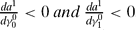Groseclose (Reference Groseclose2001) provides an influential theoretical model with policy-motivated candidates and differential additive valence and uncertainty about the median voter's position. Without valence differences, the two candidates locate symmetrically around the expected median. When the valence of one of the candidates increases, the equilibrium position initially becomes more moderate before eventually (i.e., for sufficiently high valence advantage) becoming more extreme. In contrast, the disadvantaged candidate always becomes more extreme as the opponent's valence increases. Thus, his model provides an explanation for the contradictory results in empirical studies of the “marginality hypothesis” that posits that weaker candidates “moderate” their policy position in order to increase their reelection probability.

Proposition 4 shows that our model provides an alternative theory for somewhat similar results, although based on different fundamental reasons than in Groseclose (Reference Groseclose2001), where divergence arises because of policy motivation. In our model, the weaker candidate becomes more extreme (i.e., focuses more strongly on his or her strong good), whereas the effects for the candidate whose productivity increases are more subtle because competition effect and substitution effect may go in opposite directions.

Another exogenous change that one can analyze is what happens when the budget increases. In classical microeconomic household theory, a household with a homogeneous utility function always spends the same fraction of income on each good, no matter how rich the household is. The constant elasticity of substitution (CES) utility function in our canonical example is homogeneous, and, consequently, an exogenous increase of the budget would leave the budget fraction allocated to each good that is optimal for the cutoff voter unaffected. It is also easy to check that the type of the indifferent voter does not change when candidates leave their budget allocation unchanged. Thus, for homogeneous voter utility functions, a change in the government's budget does not change the equilibrium budget allocations for the two public goods (relative to the total size of the budget). This would change for nonhomogeneous voter utility functions, as in this case, an increase of the budget may affect the cutoff voter type, with corresponding changes in equilibrium platforms.

Application: Voter Preferences with Constant Elasticity of Substitution

In this section, we determine the equilibrium solution of the model for the case of utility functions with CES, given by

(6)

$\begin{equation}\label{ces} v(x_0,x_1,t)=\big((1-t)x_0^\rho+tx_1^\rho\big)^{1/\rho}, \end{equation}$

where ρ ∈ (−∞, 1]. Our main interest in this section is how properties of the voters' utility functions (in particular, the degree of substitutability between the public goods) influence whether candidates use the proposed budget allocation to strengthen their strong issue or to partially compensate for their weakness.

To understand the role of ρ, observe that the marginal rate of substitution (the slope of the indifference curve) is given by

(7)

$\begin{eqnarray}\label{ces.mrs} \frac{dx_1}{dx_0}&=& -\displaystyle\frac{(1-t) x_0^{\rho-1} \left((1-t)x_0^\rho+tx_1^\rho\right)^{\frac{1}{\rho}-1}}{t x_1^{\rho-1} \left((1-t)x_0^\rho+tx_1^\rho\right)^{\frac{1}{\rho}-1}}\nonumber\\ & =& -\displaystyle\frac{(1-t)}{t}\left(\displaystyle\frac{x_1}{x_0}\right)^{1-\rho}. \end{eqnarray}$

In the CES utility function given in Equation (6), $\frac{1}{1-\rho}$ is referred to as elasticity of substitution and measures the curvature of the voter's indifference curve. If ρ = 1, then voters are only interested in a weighted sum of x ₀ and x ₁; the weights t and 1−t differ between voters, but the slope of each voter's indifference curve is constant at $-\frac{(1-t)}{t}$ [as $(x_1/x_0)^0=1$ for all x ₀ and x ₁]. The constant marginal rate of substitution implies, for example, for voter type t = 2/3, an increase of x ₁ by one unit is always worth as much as an increase of x ₀ by two units. In contrast, for ρ < 1, the voters' marginal rate of substitution depends on x ₀ and x ₁ (as well as, of course, on t). For example, the case of ρ → 0 corresponds to Cobb-Douglas preferences, and ρ → −∞ corresponds to L-shaped “Leontief” indifference curves.Footnote ²⁵

Given policy proposals a ⁰ and a ¹, the voter who is indifferent between the two candidates is given by the value of t that solves

(8)

$\begin{eqnarray} &&\big((1-t)\big[\gamma^0_0a^0\big]^\rho+t\big[\gamma^0_1(1-a^0)\big]^\rho\big)^{1/\rho}\nonumber\\ &&\quad = \big((1-t)\big[\gamma^1_0 a^1\big]^\rho+t\big[\gamma^1_1(1-a^1)\big]^\rho\big)^{1/\rho}, \end{eqnarray}$

which is

(9)

$\begin{eqnarray}\label{taa} &&\hspace*{-8.5pt}t(a^0,a^1)\nonumber\\ &&\hspace*{-4.5pt}=\displaystyle\frac{\big(\gamma^1_0 a^1\big)^\rho -\big(\gamma^0_0 a^0\big)^{\rho}}{\big(\gamma^1_0 a^1\big)^\rho -\big(\gamma^0_0 a^0\big)^{\rho} -\big(\gamma^1_1(1-a^1))^\rho+(\gamma^0_1(1-a^0)\big)^\rho}.\nonumber\\ \end{eqnarray}$

Candidate 0's objective is to increase t(a ⁰, a ¹) as far as possible because each voter t ≤ t(a ⁰, a ¹) votes for candidate 0. Similarly, candidate 1's objective is to decrease t(a ⁰, a ¹) as far as possible, because each voter t ≥ t(a ⁰, a ¹) votes for candidate 1. As we show in the Appendix, the corresponding first-order conditions can be rearranged to yield

(10)

$\begin{equation}\label{ces.cond} \frac{\frac{1-a^0}{a^0}}{\frac{1-a^1}{a^1}} = \left[\frac{\gamma^0_1/\gamma^1_1}{\gamma^0_0/\gamma^1_0}\right]^{\frac{\rho}{1-\rho}}. \end{equation}$

Note that the term in square brackets is smaller than 1 (as γ⁰₀ > γ¹₀ and γ¹₁ > γ⁰₁). Thus, if ρ ∈ (0, 1], then the left-hand side of Equation (10) is smaller than 1, which implies a ⁰ > a ¹. Conversely, if ρ < 0, then the left-hand side of Equation (10) is greater than 1, which implies a ⁰ < a ¹, and ρ = 0 is the boundary case, where a ⁰ = a ¹.Footnote ²⁶

Proposition 5. For the class of CES utility functions given by Equation (6), the following results hold:

1. If ρ ∈(0, 1], then a ⁰ > a ¹.
2. If ρ = 0, then a ⁰ = a ¹.
3. If ρ < 0, then a ⁰ < a ¹.

proof. See the Appendix.

Thus, in cases where the two public goods are relatively good substitutes, candidates choose platforms that further strengthen their respective strong point; that is, candidate 0 chooses to put more money into the production of good 0 than candidate 1, and vice versa for good 1. In contrast, in cases where the two public goods are relatively poor substitutes, candidates choose platforms in which they compensate for their weakness; that is, each candidate puts less money than the opponent into the production of the good in which he or she is strong. This allows the candidate to spend more money on his or her weak good, partially offsetting the advantage of his or her competitor there.

It is interesting to relate the result of Proposition 5 to the literature on Riker's Dominance principle, which stipulates that candidates should campaign on issues that play to their strengths while avoiding issues that either accent the opposition's strengths or highlight their own weaknesses. Other studies suggest that candidates sometimes engage in “issue trespassing” as they campaign in their opponent's issue territory.Footnote ²⁷ Proposition 5 suggests that the dominance principle is more likely to apply in situations where the two areas are close substitutes.

We should, however, point out three caveats. First, even in the case that ρ < 0 and therefore a ⁰ < a ¹, it is still the case that candidate 0's platform is more attractive for those voters who care predominantly about good 0, and vice versa. Issue trespassing in our model (if we want to interpret the ρ < 0 case as such) never impresses the most avid natural supporters of candidates to vote for their opponents; rather, it is always aimed at moderates (i.e., the cutoff voter) in order to convince them that the candidate's disadvantage in this policy area would be small. Second, comparing across campaign situations with different degrees of substitutability may not be quite so straightforward because when goods are close substitutes for voters, it appears plausible that candidates may not differ too much in their area-specific productivity.

Third, and more fundamentally, our model speaks to candidate positioning, whereas most of the empirical campaigning literature focuses on campaign strategies (i.e., which topics are covered by candidate advertisements). It is certainly plausible that candidates focus more on their strong topics in order to increase the salience of these topics for the electorate. Yet, it is probably also not optimal for a candidate to cede the field completely on his or her “weak” issues. What our model contributes to this literature is a rationale for why there are “strong” and “weak” issues, and, in particular, why a candidate cannot simply eliminate his or her weakness by copying the opponent's position.

We now turn to an analysis of equilibrium existence conditions. It is useful to assume a symmetric ability distribution such that γ⁰₀ = γ¹₁ = r and γ⁰₁ = γ¹₀ = 1−r, where r ≥ 0.5 measures the extent of (symmetric) specialization. If r is close to 1/2, then a candidate's advantage in his or her better field is very limited, whereas if r is high, then each candidate is a specialist in his or her strong field and a rookie in the other field.

We know from Proposition 1 that candidates choose positions that maximize the utility of the cutoff voter. Maximizing

(11)

$\begin{equation}\label{ces.2} [(1-t)(r a^0)^\rho+t((1-r)(1-a^0))^\rho]^{1/\rho} \end{equation}$

with respect to a ⁰ for candidate 0 and an analogous problem for candidate 1, and substituting t=1/2 (because of the symmetry of the problem, the cutoff voter must be located at 1/2) yields

(12)

$\begin{equation}\label{ex.sol.3} \bar a^{0}=\frac{1}{1+ \big(\frac{1-r}{r}\big)^\frac{\rho}{1-\rho}}, \quad \bar a^{1}= \frac{\big(\frac{1-r}{r}\big)^\frac{\rho}{1-\rho}}{1+\big(\frac{1-r}{r}\big)^\frac{\rho}{1-\rho}}. \end{equation}$

The corresponding production levels are

(13)

$\begin{eqnarray} \label{ex.sol.x} \bar x_0^0=\bar x_1^1= \frac{r}{1+ \big(\frac{1-r}{r}\big)^\frac{\rho}{1-\rho}} \text{,} \bar x_1^0=\bar x_0^1= \frac{(1-r)\big(\frac{1-r}{r}\big)^\frac{\rho}{1-\rho}}{1+ \big(\frac{1-r}{r}\big)^\frac{\rho}{1-\rho}}.\nonumber\\ \end{eqnarray}$

Suppose (without loss of generality) that F(0.5) ≥ 0.5. Because candidate 0 wins with probability F(0.5) if both candidates play according to Equation (12), we know from Proposition 2 that candidate 0 has no incentive to deviate. Thus, we can focus on candidate 1.

Figure 4 provides the cutoff individual as a function of candidate 1's budget allocation a ¹ for ρ = 0.5 and r = 0.55 (i.e., very moderate specialization of candidates). For low values of a ¹ (a ¹ < 0.6318), candidate 1 attracts all voters located above the cutoff. Consequently, candidate 1's set of supporters is maximized (in this range) by a ¹ = 0.45, for which the cutoff is 0.5. This, of course, is just ā ¹ given in Equation (12). Allocating slightly more money to good 0 production just loses moderate voters (i.e., the cutoff goes up). For a ¹ ∈ [0.6318, 0.6722],Footnote ²⁸ all voters prefer candidate 0. The outflanking deviations start from a ¹ > 0.6722. Candidate 1 now appeals to voter types below the cutoff (i.e., those voters who care primarily about good 0). Thus, it is optimal for candidate 1 to maximize the cutoff in this range. This is achieved by setting a ¹ ≈ 0.8195, which generates a cutoff of slightly less than 0.298, so that candidate 1's winning probability with the optimal deviation is about F(0.298). Thus, if 1−F(0.5) > F(0.298) (i.e., if the probability that the median voter is a type larger than 0.5 is larger than the probability that the median voter type is below 0.298), then even the optimal deviation decreases candidate 1's winning probability.

FIGURE 4.

Cutoff as Function of Candidate 1's Choice of a ¹ (r = 0.55, ρ = 0.5)

For example, suppose that the location of the median voter is normally distributed around 0.4 with standard deviation σ_t. For any σ_t, the actions characterized by Equation (12) are the unique equilibrium because 1−F(0.5) > F(0.298). From a welfare perspective, the equilibrium in which candidates maximize the utility of voter type 0.5 appears very inefficient: as σ_t → 0, the median voter is almost certainly close to 0.4, and candidate 0 wins the election with probability close to 1 (because he or she has a comparative advantage in the production of the good that the majority cares about more). However, he or she does so with a platform that, from a social point of view, caters too much to the interests of the (likely) minority that cares more about good 1.

EXTENSIONS

In this section, we analyze the robustness of the model with respect to three important extensions. First, we discuss what happens when candidates are chosen by parties rather than exogenously assumed to have differential productivities. Second, we discuss what happens when candidates can choose the tax rate as part of their platform (in addition to the budget allocation). Third, we present an important re-interpretation, in which the goods in the model are interpreted as intermediate goods that enter in the production of a final good.

Party Choice of Candidates. A key ingredient of our model is that candidates have differentiated abilities. Because the nature of the equilibrium differs considerably when both candidates have the same abilities, it is important to discuss whether parties will nominate candidates with differential abilities. An earlier working paper version of this article, available from the authors on request, provides some formal analysis of this extension and argues that parties are likely to nominate differentiated candidates.

There are two interrelated reasons for this. First, for the party that consists of members with an above-average preference for good 0, choosing a candidate who is particularly skilled in the provision of good 0 has the advantage that this candidate will compete in the general election with a platform that focuses on this strength, whereas choosing a candidate who is skilled in good 0 provision (and not so great in good 1 provision) is a commitment device that ensures that the candidate does not deviate too much from the policy focus preferred by members. Second, although candidates in our model are purely office motivated, it appears plausible that ordinary party members care more about policy. In this case, party members may be willing to nominate a more specialized candidate even if that decreases the party's winning probability because, as argued previously, if elected, a more specialized candidate implements a platform that is strongly preferred by party members.

Endogenous Taxation. In the basic model, we assume that both candidates raise the same taxes and thus face the same budget constraint. In case the level of taxation is another choice variable for candidates, a voter's preferences depend on two parameters: how much the voter cares about the two goods (just as in the basic model), and the voter's income. When candidates propose different tax rates, the analysis potentially becomes considerably more complicated because changing the tax rate affects a cutoff curve rather than just shifting a cutoff type in a one-dimensional parameter space.

A full analysis is beyond the scope of this article. However, in the working paper version available on the authors' homepage, we show that there is a relatively large class of utility functions for which the results of the basic model extend in a very straightforward way. Specifically, we analyze the case that voter utility is additively separable into a logarithmic utility from private consumption and a homogeneous utility function over the two public goods. We show that both candidates choose the same tax rate even if the candidates' productivities are asymmetric. Consequently, the budget allocation choice is determined in exactly the same way as in the basic model.

Uncertainty and Disagreement about the Production Process of Public Goods. Our model can be reinterpreted as one in which only one ultimate public good is provided, and all voters just want the highest quantity possible. However, there is disagreement among voters on how the ultimate public good is provided from two intermediate goods.

Consider the following example. The ultimate public good that all voters care about is “national security.” The two main inputs that affect the level of national security are “international goodwill” and “military power.” International goodwill reduces the likelihood that other actors such as foreign states or ethnic or religious communities want to undertake aggressive actions. Military power works as a deterrent and increases our ability to deal with an aggressive move, should one occur. Both “international goodwill” and “military power” can be increased by spending money on, say, development aid or military hardware, respectively. However, it is also quite plausible that the identity of the winning candidate matters. For example, in the last presidential election Obama was generally believed to be able to provide more “international goodwill” than McCain. It is also plausible that, because of his military background, a majority of voters believed that McCain had a competency advantage in increasing “military power.”

This model is analytically equivalent to the two goods setup that we analyze. In our formal model, citizens directly derive utility from two public goods, and a parameter measures how much they care about each good. A key role for the analysis is played by the voters' indifference curves (i.e., all those combinations of the public goods that lead to the same utility for a voter). In the intermediate goods scenario, voters differ in how effective they believe that certain intermediate goods are at producing the ultimate good; thus, each voter's indifference curves in this scenario are effectively the “isoquants” of the production process in which the voter believes.

During the campaign, candidates can make policy proposals that imply how much they would invest in the two intermediate goods. Voters who believe that military power matters most for national security will prefer the candidate whose platform offers more of it, and vice versa for those who believe that international goodwill is more important. Conversely, candidates have an incentive to offer a platform that emphasizes their strength (with respect to the intermediate good that they are better at producing).

We should note that game theorists sometimes find it problematic to assume that agents differ in their beliefs about how the world works (the “common prior assumption” in game theory). Yet, in practice, the phenomenon that actors genuinely disagree about complex causation mechanisms appears to be widespread. Because the national security outcome is a very complex and long-term process, we would argue that it is quite plausible that voters have substantial and stable differences of opinion about how international goodwill and military power interact in generating national security. Even though they may genuinely be interested in the same ultimate outcome, some voters may believe that what matters is primarily hard military power, whereas others may believe that international goodwill matters substantially, too.

CONCLUSION

In this article, we developed a formal model of political competition between candidates with heterogeneous capabilities in different policy fields. Candidates are office motivated and compete by proposing how to allocate government resources to different policy fields. The model has a unique equilibrium that differs substantially from the standard one-dimensional model. Although candidates compete for the support of a moderate voter type, this cutoff voter differs from the expected median voter. Moreover, no voter type, except the cutoff voter, is indifferent between the candidates in equilibrium. The model predicts that candidates respond to changes in the preferences of voters in a very rigid way. We also analyze under which conditions candidates choose to strengthen the issues in which they have a competency advantage, and when they choose to compensate for their weaknesses.

Finally, we show that when parties can choose the qualities of their nominee, they have an incentive to go for a candidate who is a specialist in the production of the good that party members care about more, rather than a balanced generalist. This is because parties know that their candidate will eventually choose a platform to appeal to a moderate cutoff voter, but the more specialized the candidate is in the production of the good that party members care about most, the more he or she will provide of that good in equilibrium.

Our model opens up several avenues for future research. We already discussed in the second section of this article how our model can inform empirical studies. One interesting theoretical issue is the nature of political campaigning in our framework. When candidates “own” certain issues, we would expect that candidates focus their campaign rhetoric on their strong issue and rarely talk about the issue in which they are weaker than their opponent. This corresponds to what William Riker called the “dominance principle” in campaign rhetoric: “When one side dominates the volume of rhetorical appeals on a particular theme, the other side abandons appeals on that theme” (Reference Riker1996, 6). As a consequence, candidates rarely engage in “dialogue” in a campaign (Simon Reference Simon2002).

In our framework, candidates cannot gain votes through pandering to marginal supporters of their opponent. Therefore, an attractive option for a campaign may be to persuade voters that the issue in which the candidate has an advantage is “really important” (in the sense of trying to influence the t in voters' utility functions). In this respect, it may be useful to combine our framework with the campaign model of Hammond and Humes (Reference Hammond, Humes and Grofman1993).Footnote ²⁹

APPENDIX

Theorem 1. Suppose that utility v(x, t) is continuous in t and x, strictly monotone, and strictly quasiconcave in x, and satisfies the single-crossing property: Footnote ³⁰

(14)

$\begin{equation} \label{single.crossing} \frac{\partial}{\partial t}\left[\frac{ \frac{\partial v(x_0,x_1,t)}{\partial x_0} } {\frac{\partial v(x_0,x_1,t)}{\partial x_1} } \right]<0. \end{equation}$

Assume that candidate j has a relative advantage in providing good j (i.e., $\gamma^j_j>\gamma^i_j$ for $i\not=j$ ). Let ξ be a lower bound for the elasticity of substitution for all consumption bundles (x ₀, x ₁) and all types t. Suppose that

(15)

$\begin{equation} \label{thm.div.cond} \left(\frac{\gamma^0_0\gamma^1_1}{\big(\gamma^1_1-\gamma^0_1\big)\big(\gamma^0_0-\gamma^1_0\big)}\right)^{1/\xi} \leq \min\left\{\frac{\gamma^1_1}{\gamma^0_1},\frac{\gamma^0_0}{\gamma^0_1}\right\}. \end{equation}$

Then there exists a pure strategy Nash equilibrium with the following properties:

1. There exists a voter type t who is indifferent between candidates 0 and 1; all types t < t strictly prefer candidate 0, and all types t > t strictly prefer candidate 1.
2. Both candidates' equilibrium strategies maximize the utility of voter t.
3. The equilibrium strategies are independent of the distribution μ of voter types.
4. Candidate 0 provides strictly more of public good 0 than candidate 1, whereas candidate 1 provides strictly more of public good 1 than candidate 0.

Lemma 1 is used in the proof of Theorem 1.

Lemma 1. Let x ⁰, x ¹ be the amount of public goods offered by the two candidates. Let D = {t|v(x ^j, t) ≥ v(x ^−j, t)} be the set of types t that weakly prefer x ^j to x ^−j. Then D is an interval. Moreover, if D ≠ [0, 1], then v(x ^j, t) = v(x ^−j, t) only for the endpoint of the interval D that is strictly inside [0, 1].

Proof of Lemma 1. Suppose by way of contradiction that D is not an interval for some x ^j, x ^−j. Note that we must have x ^j ≠ x ^−j, else D = [0, 1]. Then there exist t < t′ < t″ such that t, t″ ∈ D but t′ ∉ D. Continuity of utility in t implies that there exists t ₀ < t ₁ such that v(x ^j, t ₀) = v(x ^−j, t ₀) and v(x ^j, t ₁) = v(x ^−j, t ₁). Thus, the indifference curves of voters t ₀ and t ₁ intersect twice, which is a contradiction to Equation (14). Hence, D is an interval.

Moreover, if D ≠ [0, 1], then the preceding argument also implies that there cannot be two different types in D that are indifferent between x ⁰ and x ¹.

Proof of Theorem 1. Let

(16)

$\begin{equation} \label{def.Hfunct} H^j(t)=\max_{a\in[0,1]} v(G^j_0(a),G^j_1(a),t). \end{equation}$

We first focus on what turns out to be the “interesting case,” where no candidate can attract all voters [i.e., suppose that H ⁰(0) > H ¹(0) and H ⁰(1) < H ¹(1)]. Continuity of H ^j, j = 0, 1 therefore implies that there exists t such that H ⁰(t) = H ¹(t). Let x ^j, i = 0, 1, be the output of public goods and ā ^j be the optimal allocation of the input, that is,

(17)

$\begin{equation} \label{def.x_bar} H^j(\bar t)=v(x^j,\bar t),\quad \bar x^j_0=G^j_0(\bar a^j), \quad x^j_1=G^j_1(\bar a^j). \end{equation}$

We now show that ā ^j, i = 0, 1 is an equilibrium.

Suppose by way of contradiction that candidate 1 can improve by deviating to producing ¹. Let D = {t|v(¹, t) ≥ v(x ⁰, t)}. If 1 ∈ D, then D is of the form [, 1], where ≥ t. (Suppose otherwise; then, by Lemma 1, v(¹, t) > v(x ⁰, t), which contradicts Equation (17) (i.e., that x ¹ maximizes the utility of type t). Thus, a deviation such that 1 ∈ D cannot increase candidate 1's winning probability because the set of types that vote for candidate 1 is weakly smaller. Hence, the following claim completes the proof that candidate 1 has no profitable deviation.

Claim 1. 1 ∈ D. Figure 5 illustrates the intuition for the proof. The left panel of Figure 5 illustrates the relationship between type t's indifference curve and the equilibrium production levels x ⁰ and x ¹ of both candidates. Clearly, the indifference curve must be tangent to the transformation frontier at both points. Suppose that x ⁰ is to the right of ⁰ as depicted in the left panel. It is then immediate that type 0, whose dashed indifference curve is steeper than that of type t, is strictly better off with x ⁰ than with any public good bundle that candidate 1 could offer. Hence, type 0 would never vote for candidate 1. Because D must either contain type 0 or type 1 by Lemma 1, this implies that 1 ∈ D. Thus, to conclude the proof we must exclude the scenario depicted in the right panel of Figure 5, where x ⁰ is to the left of ⁰. If the goods are sufficiently well substitutable [i.e., if (15) holds], then this limits the amount by which the marginal rate of substitution (MRS) can change along the indifference curve (the limit on the change of the MRS can be related to a lower bound on the elasticity of substitution). In particular, suppose we move along the indifference curve of type t, starting from x ⁰ and ending at the intersection with the dashed line ξ. If the MRS at this intersection is still less than Δ, then ¹ is above the indifference curve, as indicated in the right panel. This, however, means that voter t is not indifferent between the candidates. Candidate 1 could find a policy, such as ¹, that would make t strictly prefer candidate 1, which cannot be the case in equilibrium. We now proceed to the formal proof.

FIGURE 5.

Illustration of the Proof of Claim 1 in Theorem 1

Proof of Claim 1. It is easy to check that candidate j's transformation frontier is

(18)

$\begin{equation} \label{tf} {\rm TF}^j=\left\{\big(x^j_0,x^j_1\big)\in\mathbb{R}^2_+ \Bigm| x_1^j=\gamma^j_1-\frac{\gamma^j_1}{\gamma^j_0} x_0^j\right\}. \end{equation}$

Because x ^j satisfies Equation (17), it follows that the marginal rate of substitution of voter t must equal negative of the slope of the transformation frontier:

(19)

$\begin{equation} \label{eq.mrs.opt} {\rm MRS}_{\bar t} (\bar x^j) = \frac{\gamma^j_1}{\gamma^j_0}. \end{equation}$

The maximum amount of good 0 that candidate 1 can provide is γ¹₀. Let ⁰ ∈ TF⁰ be

(20)

$\begin{equation} \label{tilde.x0} \tilde x^0_0=\gamma^1_0,\quad \tilde x^0_1=\gamma^0_1\left[1-\frac{\gamma^1_0}{\gamma^0_0}\right]. \end{equation}$

Similarly, the maximum amount of good 1 that candidate 0 can provide is γ⁰₁. Let ¹ ∈ TF¹ be

(21)

$\begin{equation} \label{tilde.x1} \tilde x^1_0=\gamma^1_0\left[1-\frac{\gamma^0_1}{\gamma^1_1}\right],\quad \tilde x^1_1=\gamma^0_1. \end{equation}$

For 0 ∈ D, we now show that x ⁰₀ < ⁰₀ must hold. To see this, note that no point on the transformation frontier of candidate 1 is strictly preferred to x ⁰ by voter t. The single-crossing property in Equation (14) therefore implies that v(x ¹, 0) < v ₀(x ₀, 0) for any point x ¹ with x ¹₀ ≤ x ⁰₀. Thus, a necessary condition for the deviation to attract type 0 is that x ⁰₀ < ⁰₀.

Let L = {α⁰ + (1 − α)¹|0 < α < 1} be the open line segment connecting ⁰ and ¹, so that

(22)

$\begin{equation} \label{def.Delta} \Delta=-\frac{\tilde x^1_1-\tilde x^0_1}{\tilde x^1_0-\tilde x^0_0} \end{equation}$

is the (negative of the) slope of this line segment.

We next show that

(23)

$\begin{equation} \label{MRS.gr.delta} {\rm MRS}_{\bar t} (\tilde x^1)\geq\Delta. \end{equation}$

Suppose by way of contradiction that MRS_t(¹) < Δ. Then quasiconcavity of utility implies that

(24)

$\begin{equation} \label{MRS.gr.delta.1} v(\tilde x^1,\bar t)>v(x,\bar t)\text{for all}x\in L. \end{equation}$

Recall that if 0 ∈ D then x ⁰₀ < ⁰₀ must hold. Furthermore, ¹₀ < x ⁰₀ because candidate 0 is better at providing good 0. Thus, there exists x ∈ L with x ≥ x ⁰. Monotonicity of preferences implies that v(x ⁰, t) < v(¹, t) ≤ v(x ¹, t), where the last inequality follows from Equation (24). Thus, t is not indifferent between the candidates, and therefore not the cutoff voter, a contradiction.

Equations (20), (21), and (22) imply

(25)

$\begin{equation} \label{MRS.ratio} \frac{\Delta} {{\rm MRS}_{\bar t} (\bar x^0)} = \frac{\gamma^1_1}{\gamma^0_1}. \end{equation}$

Furthermore, Equations (20) and (21) yield

(26)

$\begin{equation} \label{tilde_x_ratio} \frac{\tilde x^1_1/\tilde x^1_0}{\tilde x^0_1/\tilde x^0_0}= \frac{\gamma^0_0\gamma^1_1}{\big(\gamma^0_1-\gamma^1_1\big)\big(\gamma^1_0-\gamma^0_0\big)}. \end{equation}$

Let (x ₁/x ₀)(MRS) be the good ratio x ₁/x ₀ on Ī as a function of the MRS. Because ξ is a lower bound for the elasticity of substitution, we get

(27)

$\begin{equation} \label{el.subst} \frac{\frac{(x_1/x_0)(MRS)}{d\,MRS}}{(x_1/x_0)(MRS)}\geq \frac{\xi}{MRS}. \end{equation}$

Integrating both sides of Equation (27) from MRS_t(x ⁰) to Δ and taking the exponential yields,

(28)

$\begin{equation} \label{el.subst.2} \left(\frac{(x_1/x_0)(\Delta)}{(x_1/x_0)({\rm MRS}_{\bar t} (\bar x^0)}\right)^{1/\xi}\geq \frac{\Delta} {{\rm MRS}_{\bar t} (\bar x^0)}. \end{equation}$

By definition, (x ₁/x ₀)(MRS_t(x ⁰) = x ⁰₁/x ¹₁ [i.e., the good ratio at which the MRS of type t is MRS_t(x ⁰) must be x ⁰₁/x ¹₁]. We have shown that $\bar x^0_0<\tilde x^0_0$ if 0 ∈ D. Thus, (x ₁/x ₀)(MRS_t(x ⁰) > (x ₁/x ₀)(MRS_t(⁰). Furthermore, as indicated in the right panel of Figure 5, (x ₁/x ₀)(Δ)< $\tilde x^1_1/\tilde x^1_0$ . In particular, by construction, voter t is indifferent between the candidates. Thus, ¹ cannot be above indifference curve Ī. For this to be the case, the slope of Ī at good ratio $\tilde x^1_1/\tilde x^1_0$ must be at least Δ. Hence, Equation (28) implies

(29)

$\begin{equation} \label{eq.cont.2} \left(\frac{\tilde x^1_1/\tilde x^1_0}{\tilde x^0_1/\tilde x^0_0}\right)^{1/\xi}> \frac{\Delta} {{\rm MRS}_{\bar t} (\bar x^0)} \end{equation}$

Substituting Equations (25) and (26) into Equation (29) contradicts Equation (15). Thus, 1 ∈ D.

The proof that a deviation by candidate 0 is not optimal it similar, except that we must replace Equation (25) by

(30)

$\begin{equation} \label{MRS.ratio.2} \frac {{\rm MRS}_{\bar t} (\bar x^1)}{\Delta} = \frac{\gamma^0_0}{\gamma^0_1}. \end{equation}$

Because MRS_t(x ⁰) < MRS_t(x ¹), strict quasiconcavity implies that x ⁰₀ > x ¹₀ and x ¹₁ > x ⁰₁.

Finally, note that the distribution of types does not affect the equilibrium. This proves the first statement.

The case where H(0, c ⁰) ≤ H(0, c ¹) or H(1, c ⁰) ≥ H(1, c ¹).

Consider the first of the two scenarios as the other case is similar. Let x ¹ be the consumption bundle provided by candidate 1 that maximizes type 0's utility. Then v(x ¹, 0) ≥ v(x, 0) for any x ∈ TF⁰. The single-crossing property in Equation (14) immediately implies that v(x ¹, t) > v(x, t) for any x ∈ TF⁰ and for any t > 0, and hence all citizens t > 0 vote for candidate 1 independently of candidate 0's strategy. Thus, (x ⁰, x ¹) is a Nash equilibrium, where x ⁰ is the consumption bundle that maximizes type 0's utility on TF⁰. Clearly, x ⁰₀ > x ¹₀ and x ¹₀ < x ¹₁.

The next result shows that the equilibrium characterized in Theorem 1 is unique and strict, provided that there is sufficient uncertainty about the position of the median voter type.

Theorem 2. Suppose that the conditions of Theorem 1 hold and that the distribution of the median voter t_m has a strictly positive density on [0, 1]. Then, one of the following is true:

1. The equilibrium is strict, and it is the unique Nash equilibrium (pure or mixed).
2. One of the candidate wins with probability 1 and receives 100% of the votes in almost all states ω ∈ Ω.

Proof of Theorem 2. Let (x ⁰, x ¹) be the allocation of public goods offered by the candidates in a pure strategy equilibrium. By Lemma 1, D ⁰ = {t|v(x ⁰, t) ≥ v(x ¹, t)} and D ¹ = {t|v(x ¹, t) ≥ v(x ⁰, t)} are intervals.

First, suppose that D ⁰ = D ¹ = [0, 1]. Clearly, each candidate's winning probability is 0.5. Given the single-crossing property in Equation (14), this implies x ⁰ = x ¹. Let t _m be the realization of the median voter type, and let be the median of the distribution of t _m. Because $\gamma^j_j>\gamma^i_j$ , the transformation frontiers have different slopes. Thus, for at least one candidate, MR(x ^j) does not equal the slope of the candidate's transformation frontier. As a consequence, there exists a bundle of public goods ^j for candidate i such that v(^j, ) > v(x ^j, ) = (x ^−j). Thus, Lemma 1 implies that is in the interior of = {t|v(^j, t) ≥ v(x ^−j, t)}. Given that contains the median of the median voters in its interior, and given that the distribution of types has strictly positive density, the winning probability for candidate j is strictly increased, a contradiction to the assumption that x ⁰ = x ¹ is a Nash equilibrium. Hence, D ⁰ and D ¹ cannot both be equal to [0,1].

Next, suppose that D ⁱ consists of only a single point (i.e., D ⁱ = {0} or D ⁱ = {1}). Continuity of preferences then implies that no citizen in D ⁱ has a strict preferences for candidate i, and all of them will therefore abstain. Finally, because t _m = 0 or t _m = 1 with probability 0, this implies that the other candidate will receive a strictly positive number of votes and therefore win 100% of all votes cast.

Thus, let D ^j ≠ [0, 1] for i = 0, 1. Furthermore, by continuity of v there exists exactly one type t* for which v(x ⁰, t*) = v(x ¹, t*). Suppose by way of contradiction that H ⁰(t*) ≠ v(x ⁰, t*), where H ⁰ is defined in Equation (16). If 0 ∈ D ⁰, then Lemma 1 implies v(x ⁰, 0) > v(x ¹, 0). Hence, there exists some ⁰ such that v(⁰, 0) > v(x ¹, 0) and v(⁰, t*) > v(x ⁰, t*) = v(x ¹, t*). Thus, t* is in the interior of = {t|v(⁰, t) ≥ v(x ¹, t)}. Because 0 ∈ and is an interval, it follows that is a strict superset of D ⁰. Because the distribution of types has strictly positive density, this implies that the winning probability for candidate 0 strictly increases, a contradiction. The proof where 1 ∈ D ⁰ or agent 1 deviates is similar. Thus, the cutoff voter t* at any equilibrium must satisfy H ⁰(t*) = v(x ⁰, t*).

We now show that there exists exactly one t that solves H ⁰(t) = H ¹(t). Suppose by way of contradiction that there exist t < t′ such that H ⁰(t) = H ¹(t) and H ⁰(t′) = H ¹(t′). Then the indifference curves of type t and that of type t′ must be tangent both to TF⁰ and TF¹. This, however, is only possible if the indifference curves intersect at at least two points, contradicting the single-crossing property in Equation (14).

Given that a unique t solves H ⁰(t) = H ¹(t), the Nash equilibrium is unique among all pure strategy Nash equilibria. Now suppose that there exists a mixed strategy equilibrium. Without loss of generality, suppose that candidate 1 mixes. By selecting x ⁰, candidate 0 can ensure that at least all types t < t vote for himor her. However, because candidate 1 mixes, the candidate choose x ¹ with probability less than 1. In such a case, there exists > t such that all citizens t < vote for candidate 0, which strictly increases candidate 0's winning probability because t _m has a strictly positive density. Thus, candidate 0's winning probability in the mixed strategy equilibrium must be strictly larger than that in the pure strategy equilibrium. Similarly, it follows that candidate 1's winning probability in the mixed strategy equilibrium must be at least as large as in the pure strategy equilibrium, a contradiction because the winning probabilities must add up to 1.

Finally, the Nash equilibrium is strict because preferences are strictly quasiconcave and therefore the solution to maximization problem in Equation (16) is unique. As a consequence, any deviation by candidate 1 from x ^j to ^j implies that v _t(x ^−j) > v _t(^j). Hence, candidate i loses type t. Because the distribution of types has a strictly positive density, this implies that candidate i's winning probability strictly decreases.

Proof of Proposition 3. Denote the cutoff voter by t. Suppose candidate 0 wins. Then the median voter in state ω must be to the left of t, (i.e., t _m < t). Consider the optimal budget allocation by candidate 0 for a voter of type t. The optimization problem

(31)

$\begin{equation} \max_{a^0} v\bigl(\gamma^0_0 a^0,\gamma^0_1(1-a^0),t) \bigr) \end{equation}$

has the first-order condition

$\begin{equation} \frac{\partial v}{\partial x_0} \gamma^0_0 - \frac{\partial v}{\partial x_1} \gamma^0_1=0, \end{equation}$

which is equivalent to

(32)

$\begin{equation}\label{eq.cond} \left[\frac{ \frac{\partial v(x_0,x_1,t)}{\partial x_0} } {\frac{\partial v(x_0,x_1,t)}{\partial x_1} } \right] \gamma^0_0 - \gamma^0_1=0. \end{equation}$

By Equation (14),

$\begin{equation}\frac{\partial}{\partial t}\left[\frac{ \frac{\partial v(x_0,x_1,t)}{\partial x_0} } {\frac{\partial v(x_0,x_1,t)}{\partial x_1} } \right]<0.\end{equation}$

Because we know from Theorem 1 that, in equilibrium, Equation (32) holds for t = t, it follows that (32) is positive for all t < t. This implies that all types t < t have an optimal level of a that is greater than ā ⁰. The argument if candidate 1 wins is analogous.

Proof of Proposition 4. Consider the optimal budget allocation by candidate 1 for a type t voter:

(33)

$\begin{equation} \max v(\gamma^1_0 a^1,\gamma^1_1 (1-a^1),t). \end{equation}$

The first-order condition is

(34)

$\begin{equation}\label{foc.thm.cs} \frac{ \frac{\partial v(x_0,x_1,t)}{\partial x_0} } {\frac{\partial v_t(x_0,x_1,t)}{\partial x_1} } = \frac{\gamma^1_1}{\gamma^1_0}. \end{equation}$

By Equation (14), the left-hand side of Equation (34) is decreasing in t. Moreover, because v is concave in both arguments, it follows that the left-hand side of Equation (34) is decreasing in a ¹. Thus, a voter with a higher type t has a lower preferred value of a ¹. Because an increase in γ⁰₀ or γ⁰₁ moves the equilibrium cutoff voter to the right (i.e., increases t), and we know from Proposition 1 that candidate 1 chooses a ¹ to maximize the utility of the new cutoff voter, this proves the first part of the theorem.

The equivalent condition to Equation (34) for candidate 0 is Equation (32) in the proof of Proposition 3. Totally differentiating Equation (32) with respect to γ⁰₁ and a yields

(35)

$\begin{equation} \frac{\partial}{\partial a} \left(\frac{\frac{\partial v}{\partial x_0}}{\frac{\partial v}{\partial x_1}}\right) da + \left[ \frac{\partial}{\partial t} \left(\frac{\frac{\partial v}{\partial x_0}}{\frac{\partial v}{\partial x_1}}\right) \frac{d\bar{t}}{d\gamma^0_1} -\frac{1}{\gamma^0_0} \right] d\gamma^0_1 =0. \end{equation}$

The first term is negative (by the second-order condition of maximization). Furthermore, as previously argued, $\frac{\partial}{\partial t} (\frac{\frac{\partial v}{\partial x_0}}{\frac{\partial v}{\partial x_1}})$ < 0 and $\frac{d\bar{t}}{d\gamma^0_1}$ > 0, so that the term in square brackets is negative. Thus, da ⁰/dγ ⁰₁ < 0, as claimed.

Going through the same steps as done previously for γ⁰₀ yields

(36)

$\begin{equation} \frac{da^0}{d \gamma^0_0} = - \frac{\frac{\partial}{\partial t} \left(\frac{\frac{\partial v}{\partial x_0}}{\frac{\partial v}{\partial x_1}}\right) \frac{d\bar{t}}{d\gamma^0_0} +\frac{\gamma^0_1}{(\gamma^0_0)^2} }{\frac{\partial}{\partial a} \left(\frac{\frac{\partial v}{\partial x_0}}{\frac{\partial v}{\partial x_1}}\right)}{\!}. \end{equation}$

The first term in the numerator is the product of a negative and a positive number, whereas the second term is positive. Consequently, the sign of the numerator, and thus of $\frac{da^0}{d \gamma^0_0}$ , is ambiguous.

Proof of Proposition 5. Differentiating Equation (9) with respect to a ⁰ and a ¹ and canceling the respective denominators and ρ yields

(37)

$\begin{eqnarray} && (\gamma^0_1)^\rho(1-a^0)^{\rho-1}\big[\big(\gamma^0_0 a^0\big)^{\rho} - \big(\gamma^1_0 a^1\big)^\rho \big]- \big(\gamma^0_0\big)^\rho (a^0)^{\rho-1}\nonumber\\ &&\quad \times\,\big[\big(\gamma^1_1 (1-a^1)\big)^{\rho} - \big(\gamma^0_1 (1-a^0)\big)^\rho \big] = 0 \\\end{eqnarray}$

(38)

$\begin{eqnarray}\quad \times\,\big(\gamma^1_1\big)^\rho(1-a^1)^{\rho-1}\big[\big(\gamma^0_0 a^0\big)^{\rho} - \big(\gamma^1_0 a^1\big)^\rho \big]- \big(\gamma^1_0\big)^\rho (a^1)^{\rho-1}\nonumber\\ &&\quad \times\,\big[\big(\gamma^1_1 (1-a^1)\big)^{\rho} - \big(\gamma^0_1 (1-a^0)\big)^\rho \big] = 0. \end{eqnarray}$

Rearranging gives

(39)

$\begin{eqnarray} \left(\frac{\gamma^0_1}{\gamma^0_0}\right)^\rho \left(\frac{1-a^0}{a_0}\right)^{\rho-1}&=& \frac{(\gamma^1_1(1-a^1))^\rho-(\gamma^0_1(1-a^0))^\rho}{(\gamma^0_0 a^0)^{\rho}- (\gamma^1_0 a^1)^\rho}\nonumber\\ & = & \left(\frac{\gamma^1_1}{\gamma^1_0}\right)^\rho \left(\frac{1-a^1}{a_1}\right)^{\rho-1}. \end{eqnarray}$

Rearranging gives Equation (10) in the text. The remaining steps of the argument are in the main text.

Footnotes

¹ Remember that candidates are uncertain about the type distribution in society and so are uncertain about the priorities and preferences of the actual median voter.

² Policy divergence in terms of budget allocation holds “almost always.” The first exception is if both candidates have exactly the same abilities, which renders the model equivalent to the standard model with convergence to the expected median's preferred position; the second exception is if voters have an elasticity of substitution exactly equal to one (i.e., a logarithmic utility function).

³ For excellent reviews of this area, see, for example, Grofman (Reference Grofman2004), Osborne (Reference Osborne1995), and Roemer (Reference Roemer2001).

⁴ By “sincere preference” we mean that these voters would prefer a more moderate position, if the candidate were elected. What we do not mean is a voter's “strategic” preference for the disliked candidate to take a less electable position.

⁵ See http://www.urbandictionary.com/define.php?term=broderism

⁶ For a formal model that explains why supermajoritarian institutions may arise in spite of potentially detrimental welfare effects, see Messner and Polborn (Reference Messner and Polborn2004).

⁷ One of the few existing papers with non-UCR preferences and office-motivated candidates is Adams and Merrill (Reference Adams and Merrill2003), where voters have, in addition to policy preferences, a partisan preference for one candidate, but may abstain due to alienation if their preferred candidate does not provide them with sufficient utility. Another paper with non-UCR preferences is Krasa and Polborn (Reference Krasa and Polborn2009b), in which two office-motivated candidates are differentiated with respect to their ability to supply small and large quantities of a single public good. Voters differ in both income and taste for public goods. The main focus is on the determination of equilibrium tax rates and how they vary with the candidates' productivities; however, an analysis of spending allocations to different policy fields is intractable in this framework. In contrast, this article focuses on the allocation of money to different policy fields while taking the level of taxation as exogenous.

⁸ See Section 5 of Krasa and Polborn (Reference Krasa and Polborn2009a) for a probabilistic voting model that is microfounded in such a way.

⁹ More peripherally related is Gautier and Soubeyran (Reference Gautier and Soubeyran2008). They analyze a dynamic model in which candidates have differential abilities and in which public goods are somewhat durable, but in which candidates do not compete for the support of a cutoff voter (they are instead assumed to maximize the utility of the deterministic median voter in each period).

¹⁰ Generally, we use superscripts to denote the candidate and subscripts to denote the good.

¹¹ In the Appendix, we show that our qualitative results hold for a large class of preferences that satisfy a single-crossing condition such that the marginal rate of substitution between goods 0 and 1 is decreasing in t.

¹² Nothing of importance would change if, instead, there are finitely many voters.

¹³ If, in a model where the distribution of voters is known with certainty, candidate payoffs depend only on whether they win (rather than vote share), then, generically, there are many equilibria. The reason is that one candidate usually wins for sure, and thus, the policy choice of his or her opponent is indeterminate. Also, the better candidate can win with a whole set of policies. Therefore, many strategies could be part of an equilibrium when candidates care only about the probability of winning in a model with a given voter distribution. This is the reason why assuming either vote share maximization (under certainty) or uncertainty about the voter preference distribution is useful.

¹⁴ The assumption that candidates' policy choices occur simultaneously is without loss of generality because we can show that any sequential move version (say, candidate 0 chooses his or her platform before candidate 1) would lead to the same policies being chosen as in the simultaneous version.

¹⁵ If a voter is indifferent, he or she could in principle vote for any candidate or abstain. However, abstention is quite natural (e.g., in the presence of even very small voting costs).

¹⁶ That is, he or she either wins whenever t _m ≤ t*_M, plus in some states where t _m is in the neighborhood of t*_M, or whenever t _m ≥ t*_M, plus in some states where t _m is in the neighborhood of t*_M. Note that, in contrast to a deterministic model, being strictly preferred by t*_M does not guarantee an election victory in our model because the realized median voter t _m usually differs from t*_M.

¹⁷ There are two nongeneric cases in which t*_M's indifference curve is tangent to one of the production possibility lines. Even in these cases, the other candidate can deviate and improve his or her winning probability, showing again that both candidates locating at x is not an equilibrium.

¹⁸ A decrease of the set of a candidate's supporter voter types translates into a decrease of the candidate's winning probability if and only if the, density of possible median voter types is positive at t. If F′(t) = 0 (i.e., the density of possible median voter types is zero at t), then there are, in addition to the equilibrium we characterize, other equilibria (all of which have the same winning probabilities for the candidates). A sufficient condition to exclude all other equilibria is to assume that F′(t) > 0 for all t ∈ (0, 1).

¹⁹ Note that x′¹ is candidate 1's optimal outflanking deviation, because the indifference curve of type t′ is tangent to his or her production possibility frontier. Candidate 1 cannot appeal to types with flatter indifference curves (because their indifference curve through x ⁰ never touches his or her production possibility frontier).

²⁰ This argument can be generalized to show the following: consider any two-player, simultaneousmove, constant-sum game (e.g., any model of electoral competition between office-motivated candidates) that, in addition, has a unique pure strategy Nash equilibrium. Any modified game with the same payoff structure, but in which players move sequentially, has a unique subgame-perfect equilibrium in which both players, along the equilibrium path, play the same actions as in the original, simultaneous-move game.

²¹ The reason why the statements in the proposition are only true “with probability 1” (rather than “always”) is that, in principle, it is possible that the cutoff voter t is also the realized median voter. In this case, a marginal changes of policy would make a (bare) majority worse off. However, note that t _m = t occurs only with probability 0.

²² This working paper version of Krasa and Polborn (Reference Krasa and Polborn2010) contains more general results than the published version, in particular, an analysis of the case with uncertainty about voter preferences that is relevant here.

²³ If the election result is lopsided in the Calvert (Reference Calvert1985) model, then the realized median voter's preferred position may be more extreme than the platform proposed by the winning candidate, so that a majority would prefer the implementation of a more extreme platform. However, this situation certainly does not arise with probability 1, as in our model.

²⁴ More generally, Krasa and Polborn Reference Krasa and Polborn2006, Theorems 5 and 6, show that, in a class of models containing the standard model, the candidates' equilibrium platforms are competition efficient if and only if there is no uncertainty about the preferred position of the median voter.

²⁵ To see the latter, note that, for $\rho\to-\infty$, $(\frac{x_1}{x_0})^{1-\rho}$ is very large if x ₁ > x ₀ and is close to zero if x ₁ < x ₀.

²⁶ The CES utility function is not defined for ρ = 0, but it is well known that the logarithmic utility function (equivalent to a Cobb-Douglas utility function here) is a utility function with CES equal to 1 (1−ρ).

²⁷ For example, Damore (Reference Damore2004) classifies 15 % of campaign advertisements of major party presidential candidates between 1976 and 1996 as speaking to “opposition issues” (i.e., issues on which the other party is perceived as having an advantage).

²⁸ The exact boundaries of this interval are 139/220 and 121/180.

²⁹ Hammond and Humes (Reference Hammond, Humes and Grofman1993) study issue framing by candidates in a two-dimensional Euclidean model. In their model, voters are initially uninformed about candidates' (exogenous) positions, candidates can only make their position in one dimension known to voters, and voters can choose which one they want to broadcast (i.e., they can choose to frame “what the election is about”).

³⁰ See Mirrlees (Reference Mirrlees1971) and Spence (Reference Spence1974). For a use of the single-crossing property in the standard Downsian model, see Gans and Smart (Reference Gans and Smart1996).

References

REFERENCES

Adams, J., and Merrill, S.. 2003. “Voter Turnout and Candidate Strategies in American Elections.” Journal of Politics 65: 161–89.CrossRef Google Scholar

Ansolabehere, S., and Snyder, J.M.. 2000. “Valence Politics and Equilibrium in Spatial Election Models.” Public Choice 103: 327–36.CrossRef Google Scholar

Aragones, E., and Palfrey, T.R.. 2002. “Mixed Equilibrium in a Downsian Model with a Favored Candidate.” Journal of Economic Theory 103 (1): 131–61.CrossRef Google Scholar

Bernhardt, D., Duggan, J., and Squintani, F.. 2009. “The Case for Responsible Parties.” American Political Science Review 103: 570–87.CrossRef Google Scholar

Besley, T., and Coate, S.. 1997. “An Economic Model of Representative Democracy.” Quarterly Journal of Economics 112: 85–114.CrossRef Google Scholar

Budge, I. 1993. “Issues, Dimensions, and Agenda Change in Postwar Democracies: Long-term Trends in Party Election Programs and Newspaper Reports in Twenty-three Democracies.” In Agenda Formation, ed. Riker, W.H.. Ann Arbor: University of Michigan Press, 41–80.Google Scholar

Budge, I., and Farlie, D.J.. 1983. Explaining and Predicting Elections. London: Allen and Unwin.Google Scholar

Callander, S. 2005. “Electoral Competition in Heterogeneous Districts.” Journal of Political Economy 113: 1116–45.CrossRef Google Scholar

Calvert, R.L. 1985. “Robustness of the Multidimensional Voting Model: Candidate Motivations, Uncertainty, and Convergence.” American Journal of Political Science 29: 69–95.CrossRef Google Scholar

Coughlin, P. 1992. Probabilistic Voting Theory. Cambridge: Cambridge University Press.CrossRef Google Scholar

Damore, D. 2004. “The Dynamics of Issue Ownership in Presidential Campaigns.” Political Research Quarterly 57 (3): 391.CrossRef Google Scholar

Dixit, A., and Londregan, J.. 1996. “The Determinants of Success of Special Interests in Redistributive Politics.” Journal of Politics 58 (4): 1132–55.Google Scholar

Downs, A. 1957. An Economic Theory of Democracy. New York: Harper.Google Scholar

Egan, P.J. 2008. “Issue Ownership and Representation: A Theory of Legislative Responsiveness to Constituency Opinion.” New York University. Unpublished manuscript.CrossRef Google Scholar

Gans, J., and Smart, M.. 1996. “Majority Voting with Single-crossing Preferences.” Journal of Public Economics 59 (2): 219–37.CrossRef Google Scholar

Gautier, P., and Soubeyran, R.. 2008. “Political Cycles: Issue Ownership and the Opposition Advantage.” Journal of Public Economic Theory 10 (4): 685–716.Google Scholar

Grofman, B. 2004. “Downs and Two-party Convergence.” Annual Review of Political Science 7: 25–46.Google Scholar

Groseclose, T. 2001. “A Model of Candidate Location When One Candidate Has a Valence Advantage.” American Journal of Political Science 45 (4): 862–86.CrossRef Google Scholar

Hammond, T., and Humes, B.. 1993. “‘What This Campaign Is All about Is. . .’: A Rational Choice Alternative to the Downsian Spatial Model of Elections.” In Information, Participation, and Choice: An Economic Theory of Democracy in Perspective, ed. Grofman, B.. Ann Arbor: University of Michigan Press, 141–59.Google Scholar

Krasa, S., and Polborn, M.K.. 2006. “Majority-effciency and competition-effciency in a Binary Policy Model.” Institute of Governmental Studies, UC Berkeley. http://escholarship.orgucitem8jd9n1dw (accessed October 17, 2010).Google Scholar

Krasa, S., and Polborn, M.K.. 2009a. “Political Competition between Differentiated Candidates.” University of Illinois. Unpublished manuscript.Google Scholar

Krasa, S., and Polborn, M.K.. 2009b. “A Political-economy Model of Taxation and Government Expenditures with Differentiated Candidates.” University of Illinois. Unpublished manuscript.Google Scholar

Krasa, S., and Polborn, M.K.. 2010. “The Binary Policy Model.” Journal of Economic Theory 145: 661–88.CrossRef Google Scholar

Lindbeck, A., and Weibull, J.. 1987. “Balanced-budget Redistribution as the Outcome of Political Competition.” Public Choice 52: 273–97.CrossRef Google Scholar

Lindbeck, A., and Weibull, J.. 1993. “A Model of Political Equilibrium in a Representative Democracy.” Journal of Public Economics 51: 195–209.CrossRef Google Scholar

Martinelli, C. 2001. “Elections with Privately Informed Parties and Voters.” Public Choice 108 (1): 147–67.CrossRef Google Scholar

Messner, M., and Polborn, M.K.. 2004. “Voting on Majority Rules.” Review of Economic Studies 71 (1): 115–32.Google Scholar

Mirrlees, J. 1971. “An Exploration in the Theory of Optimal Income Taxation.” Review of Economic Studies 38: 175–208.CrossRef Google Scholar

Osborne, M. 1995. “Spatial Models of Political Competition under Plurality Rule: A Survey of Some Explanations of the Number of Candidates and the Positions They Take.” Canadian Journal of Economics 27: 261–301.Google Scholar

Osborne, M., and Slivinski, A.. 1996. “A Model of Political Competition with Citizen Candidates.” Quarterly Journal of Economics 111: 65–96.CrossRef Google Scholar

Palfrey, T.R. 1984. “Spatial Equilibrium with Entry.” Review of Economic Studies 51: 139–56.CrossRef Google Scholar

Petrocik, J.R. 1996. “Issue Ownership in Presidential Elections, with a 1980 Case Study.” American Journal of Political Science 40 (3): 825–50.CrossRef Google Scholar

Riker, W.H. 1993. “Rhetorical Interaction in the Ratification Campaigns.” In Agenda Formation, ed. Riker, W.H.. Ann Arbor: University of Michigan Press, 81–123.Google Scholar

Riker, W.H. 1996. The Strategy of Rhetoric. New Haven, CT: Yale University Press.Google Scholar

Roemer, J.E. 1994. “A Theory of Policy Differentiation in Single Issue Electoral Politics.” Social Choice and Welfare 11 (4): 355–80.Google Scholar

Roemer, J.E. 2001. Political Competition: Theory and Applications. Cambridge, MA: Harvard University Press.Google Scholar

Simon, A.F. 2002. The Winning Message: Candidate Behavior, Campaign Discourse, and Democracy. Cambridge: Cambridge University Press.CrossRef Google Scholar

Soubeyran, R. N.d. “Does a Disadvantaged Candidate Choose an Extremist Position?” Annales d'Economie et de Statistique, Forthcoming.Google Scholar

Spence, M. 1974. “Competitive and Optimal Responses to Signals: An Analysis of Effciency and Distribution.” Journal of Economic Theory 7: 296–332.Google Scholar

Stokes, D. 1963. “Spatial Models of Party Competition.” American Political Science Review 57 (2): 368–77.CrossRef Google Scholar

Suellentrop, C. 2004. “The Vanishing Nonvoter: Has Karl Rove Brought Too Many New People to Politics?” Slate, October 31. www.slate.comid2108924/ (accessed October 17, 2010).Google Scholar

Wittman, D. 1983. “Candidate Motivation: A Synthesis of Alternative Theories.” American Political Science Review 77: 142–57.Google Scholar

FIGURE 1.Production Possibility Sets and Nonequilibrium Choices

FIGURE 2.Equilibrium Choices

FIGURE 3.Large Policy Deviations

FIGURE 4.Cutoff as Function of Candidate 1's Choice of a1 (r = 0.55, ρ = 0.5)

FIGURE 5.Illustration of the Proof of Claim 1 in Theorem 1

Submit a response

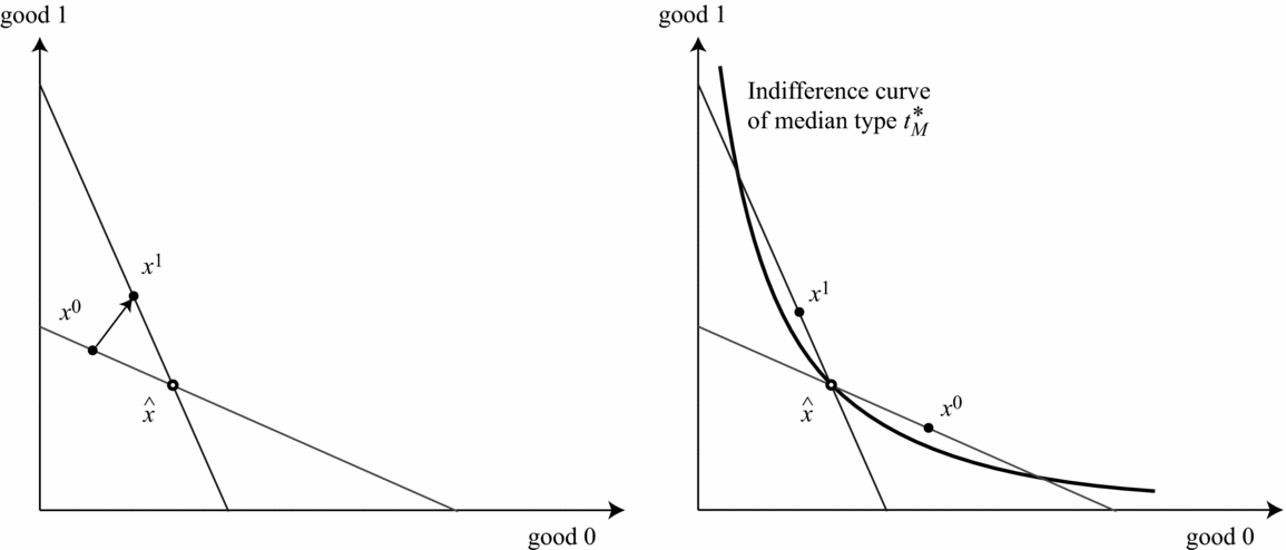
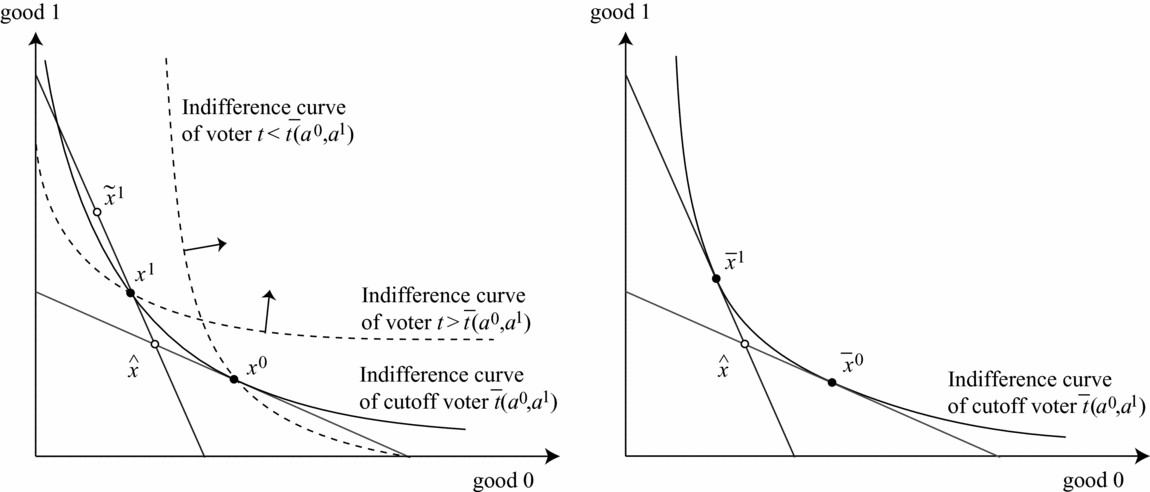
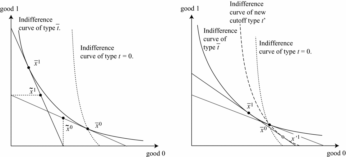
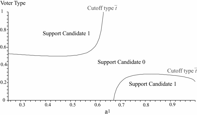
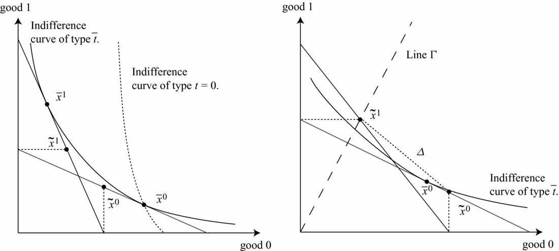
Comments

No Comments have been published for this article.

Article contents

Competition between Specialized Candidates

Abstract

Information

CAUSES AND CONSEQUENCES OF HETEROGENEOUS CANDIDATE ABILITIES

Policy Areas and Differences between Candidates

Heterogeneous Candidates Competing for Voters

Equilibrium Properties and Comparison to the Literature

RELATED LITERATURE

MODEL

RESULTS

Equilibrium

Welfare

Comparative Statics

Application: Voter Preferences with Constant Elasticity of Substitution

EXTENSIONS

CONCLUSION

APPENDIX

Footnotes

References

REFERENCES

Comments

Save article to Kindle

Save article to Dropbox

Save article to Google Drive

Reply to: Submit a response

Your details

You have entered the maximum number of contributors

Conflicting interests