



1 Introduction
The rotating-disc boundary layer may be regarded as providing a prototypical configuration for studies of the instability mechanisms that can trigger laminar–turbulent transition in three-dimensional wall-bounded external flows. It is formed when a planar solid surface is rotated, with a constant angular velocity, to drive the motion of an otherwise unbounded region of incompressible fluid that lies immediately above it. This relatively simple rotating flow was first identified and described almost a century ago by von Kármán (Reference von Kármán1921). Since that time, it has been the frequent subject of investigations, conducted using a variety of theoretical, numerical and experimental methods (Lingwood & Alfredsson Reference Lingwood and Alfredsson2015). In recent years, attention has focused on the nature of the global stability behaviour which is displayed in the spatial and temporal development of linearised forms of disturbance. This interest was provoked by the discovery that the boundary layer is susceptible to an absolute form of instability (Lingwood Reference Lingwood1995, Reference Lingwood1996). However, the occurrence of such an instability was only theoretically demonstrated within the context of a mathematical approximation. In order to simplify the analysis and make it more tractable, the genuine flow was replaced by an artificial version obtained by means of a radial homogenisation. In the present paper, we will reconsider the connections that may be exhibited between absolute instability and the global features of the linearised disturbance development for the exact, radially inhomogeneous, base flow.
Previous studies have shown that, despite the presence of an absolute instability mechanism, the effects associated with the radial inhomogeneity of the genuine flow can become strong enough to lead to a global stabilisation of disturbances (Davies & Carpenter Reference Davies and Carpenter2003; Davies, Thomas & Carpenter Reference Davies, Thomas and Carpenter2007). This was carefully documented for the disturbance development over a wide range of radial locations, when the azimuthal mode number was chosen to be broadly comparable to the critical value for the onset of absolute instability. It was later demonstrated that such strong effects on the global stability behaviour were persistent across a variety of related rotating-disc boundary layers, for which the physical configuration of the basic state was taken to be amended in some manner. These modified flows comprised cases where there was either mass transfer at the disc surface, an imposed axial magnetic field, or the fluid was allowed to rotate at large distances above the disc (Thomas & Davies Reference Thomas and Davies2010, Reference Thomas and Davies2013; Davies & Thomas Reference Davies and Thomas2017). In some instances, it was discovered that the radial inhomogeneity could give rise to globally unstable behaviour, rather than promoting stability, which was characterised by a faster than exponential temporal growth for disturbances triggered by a spatially localised impulsive forcing. However, Thomas and Davies were unable to locate any fixed global temporal frequency, which might have been anticipated for a globally unstable flow. Instead, for the time duration that disturbance development could be accurately simulated, temporal frequencies were found to vary in both the radial direction and with time.
Excellent reviews on global instability concepts and globally unstable flows are presented by Huerre & Monkewitz (Reference Huerre and Monkewitz1990), Huerre (Reference Huerre, Batchelor, Moffatt and Worster2000) and Schmid & Henningson (Reference Schmid and Henningson2001). The global instability of numerous wake flows has been investigated by Hannemann & Oertel (Reference Hannemann and Oertel1990), Oertel (Reference Oertel1990), Zielinska & Westfried (Reference Zielinska and Westfried1995), Leu & Ho (Reference Leu and Ho2000) and reviewed by Huerre & Monkewitz (Reference Huerre and Monkewitz1990). Further examples of flows exhibiting globally unstable properties include some jet and plume flows (again reviewed by Huerre & Monkewitz Reference Huerre and Monkewitz1990) and the flickering candle (Maxworthy Reference Maxworthy1999).
For the subsequent study we will show that the same form of rapid temporal growth observed by Thomas & Davies (Reference Thomas and Davies2010) on the rotating-disc with mass suction, can also be identified for the unmodified infinite rotating-disc boundary layer. However, it is only found when the azimuthal mode number of the disturbance is taken to be significantly greater than the values, selected to yield near criticality for the occurrence of absolute instability, that were the primary focus of previous investigations. Thus, globally unstable characteristics appear outside the parameter range that had been presumed to be the most relevant for studying its possible onset.
Absolute instability in the rotating-disc boundary layer was discovered by Lingwood (Reference Lingwood1995) using the Briggs (Reference Briggs1964) pinch-point method. It was shown that this form of instability is generated by the coalescence of the cross-flow instability (Gregory, Stuart & Walker Reference Gregory, Stuart and Walker1955) and a spatially damped mode that propagates radially inwards (Mack Reference Mack1985). At least one other form of instability exists within the von Kármán flow that is a direct consequence of the Coriolis forces present in rotating boundary layers (Faller & Kaylor Reference Faller and Kaylor1966; Malik Reference Malik1986). Critical absolute instability was identified by Lingwood (Reference Lingwood1995) for Reynolds numbers
 $Re_{a}\geqslant 507.3$
, whilst experimental observations indicate that transition to turbulence sets in for Reynolds numbers
 $500\leqslant Re_{t}\leqslant 560$
(Gregory et al.
Reference Gregory, Stuart and Walker1955; Gregory & Walker Reference Gregory and Walker1960; Kobayashi, Kohama & Takamadate Reference Kobayashi, Kohama and Takamadate1980; Malik, Wilkinson & Orszag Reference Malik, Wilkinson and Orszag1981; Wilkinson & Malik Reference Wilkinson and Malik1985; Lingwood Reference Lingwood1996; Othman & Corke Reference Othman and Corke2006; Imayama, Alfredsson & Lingwood Reference Imayama, Alfredsson and Lingwood2012, Reference Imayama, Alfredsson and Lingwood2013, Reference Imayama, Alfredsson and Lingwood2014). Given the apparent consistency in the onset of transition and the appearance of absolute instability, Lingwood suggested that absolute instability may be responsible for the breakdown of laminarity in the rotating-disc boundary layer. However, Davies & Carpenter (Reference Davies and Carpenter2003) inferred that absolute instability was not sufficient to excite globally unstable disturbances. Furthermore, Lingwood (Reference Lingwood1996) was unable to identify a dominant frequency that may have been anticipated if the absolute instability were to establish a temporally growing global mode.
Using solutions of the linearised complex Ginzburg–Landau equation (originally derived by Hunt & Crighton Reference Hunt and Crighton1991), Davies et al. (Reference Davies, Thomas and Carpenter2007) were able to show that the global behaviour depicted by Davies & Carpenter (Reference Davies and Carpenter2003) arises due to a ‘detuning’ effect that is a result of a radially varying complex temporal frequency. Depending on the precise relationship between the radial variations in frequency and growth rate (and diffusion/dispersion effects), the flow could remain globally stable despite being locally absolutely unstable. Stabilisation by detuning has been familiar to many in the astrophysical fluids research community for quite some time and is better known as ‘phase mixing’ (Soward Reference Soward1977, Reference Soward1992; Harris, Bassom & Soward Reference Harris, Bassom and Soward2000).
Davies and co-workers (Davies & Carpenter Reference Davies and Carpenter2003; Davies et al.
Reference Davies, Thomas and Carpenter2007) discuss the interpretation of the temporal frequency based on a local and global time non-dimensionalisation. The former scaling is based on the ratio of the constant boundary layer thickness and the circumferential speed of the rotating-disc while the global time scale is defined by taking the inverse of the disc angular velocity. Thus, the globally scaled temporal frequency
 $g=fRe$
, where
 $Re$
is the Reynolds number and
 $f$
is the locally scaled frequency that is more commonly utilised in stability investigations based on a radial homogeneous approximation of the basic state. Additionally, an integer-valued azimuthal mode number is defined as
 $n=\unicode[STIX]{x1D6FD}Re$
, where the azimuthal wavenumber
 $\unicode[STIX]{x1D6FD}$
is treated as a continuous parameter in local stability analysis. For solutions to the homogeneous flow, the temporal frequency
 $g_{r}$
and growth rate
 $g_{i}$
can then be mapped on to the
 $\{Re,n\}$
-parameter space. (Note that subscripts
 $r$
and
 $i$
denote the real and imaginary parts of
 $g$
.) Contours of
 $g_{r}$
and
 $g_{i}$
are plotted in figure 1, which are consistent with the calculations given by Lingwood (Reference Lingwood1995) and the illustrations of Pier (Reference Pier2003). For a fixed value of
 $n\geqslant 51$
absolutely unstable behaviour is only found for a finite range of Reynolds numbers. For instance, at
 $n_{a}=68$
(critical azimuthal mode number for absolute instability) disturbances are absolutely unstable over the parameter range
 $507\lesssim Re\lesssim 1600$
. For larger Reynolds numbers disturbances are either convectively unstable or stable. Furthermore, temporal growth rates vary approximately quadratically, while the matching frequencies increase linearly with the Reynolds number (Davies et al.
Reference Davies, Thomas and Carpenter2007; Thomas Reference Thomas2007; Healey Reference Healey2010).
Contours of the (a) temporal frequency
 $g_{r}$
and (b) growth rate
 $g_{i}$
in the
 $\{Re,n\}$
-parameter space, based on solutions of the radially homogeneous base flow. Horizontal lines correspond to modes
 $n_{a}=68$
(dashed) and
 $n=51$
(dotted).

Recent studies on the von Kármán flow have examined finite disc effects. Utilising the modelling work of the Davies group and solutions of the Ginzburg–Landau equation, Healey (Reference Healey2010) argued that for a disc of finite radius, absolute instability could establish globally unstable disturbances. However, experiments by Imayama et al. (Reference Imayama, Alfredsson and Lingwood2013) were unable to confirm a direct relationship between the onset of transition and the Reynolds number at the edge of the disc. Instead it was suggested that the scatter of reported transition Reynolds numbers could be explained by the different interpretations for transition. Pier (Reference Pier2013) undertook a similar experimental investigation on the rotating-disc and the effects, if any, of a finite radial domain. He found that the edge of the disc could act as a source for strong fluctuations and that the apparent inconsistencies between the analysis of Healey (Reference Healey2010) and Imayama et al. (Reference Imayama, Alfredsson and Lingwood2013) could be reconciled if the downstream boundary was modelled as a source of random noise.
Appelquist et al. (Reference Appelquist, Schlatter, Alfredsson and Lingwood2015a
,Reference Appelquist, Schlatter, Alfredsson and Lingwood
b
, Reference Appelquist, Schlatter, Alfredsson and Lingwood2016) used numerical simulations to undertake both a linear and nonlinear study on the disturbance development on a finite rotating-disc for azimuthal mode numbers near critical conditions for absolute instability. The original calculations of Davies & Carpenter (Reference Davies and Carpenter2003) were extended to longer time periods, and finite disc effects were modelled by accounting for downstream turbulence. Inwardly travelling perturbations were excited by a turbulent outer ring that led to the creation of a form of global instability that was characterised by the conditions at the outer boundary of the radial domain. If the pocket of local absolute instability was sufficiently large, globally unstable disturbances could be established. A globally unstable mode was found for
 $n_{a}=68$
and
 $Re_{cg}=583$
. Extrapolating their analysis of finite discs through to a rotating-disc of infinite extent (as undertaken by Davies & Carpenter Reference Davies and Carpenter2003), Appelquist et al. confirmed (for azimuthal mode numbers near the onset of absolute instability) that the infinitely large rotating-disc is globally linearly stable. More recently, Appelquist et al. (Reference Appelquist, Schlatter, Alfredsson and Lingwood2018) simulated stationary convective instabilities excited by surface roughness on a finite disc. Disturbance development was tracked through the linear and nonlinear stages of transition. For all simulations modelled, turbulence was attained before
 $Re_{cg}$
, meaning that the primary instability was convective in nature. Secondary instabilities were triggered and different transition scenarios realised, depending on the initial roughness amplitude.
In this paper we will focus on the global linear stability characteristics on the infinite rotating-disc and consider a possible oversight by previous studies regarding the requirements for global instability. Using solutions of the linearised Ginzburg–Landau equation with linearly varying coefficients, Chomaz, Huerre & Redekopp (Reference Chomaz, Huerre and Redekopp1988) found that a region of local absolute instability is a necessary but not sufficient condition for global linearly unstable behaviour (Huerre & Monkewitz Reference Huerre and Monkewitz1990; Huerre Reference Huerre, Batchelor, Moffatt and Worster2000). In order for global instability to develop the region of absolute instability had to exceed a critical size (Chomaz et al.
Reference Chomaz, Huerre and Redekopp1988; Huerre & Monkewitz Reference Huerre and Monkewitz1990; Huerre Reference Huerre, Batchelor, Moffatt and Worster2000). The von Kármán flow is only absolutely unstable over a finite range of Reynolds numbers (or radii) for any fixed azimuthal mode number
 $n\geqslant 51$
, with the region of absolute instability increasing for larger
 $n$
(figure 1
b). Previous studies of the infinite rotating-disc, that focused on the first azimuthal mode numbers to become absolutely unstable, have only observed globally stable characteristics. In other words the absolutely unstable mechanism was not sufficient to generate global instability. Davies & Carpenter (Reference Davies and Carpenter2003) considered the evolution of disturbances over the parameter range
 $n\in [30:75]$
, while Appelquist et al. (Reference Appelquist, Schlatter, Alfredsson and Lingwood2015a
) modelled the
 $n_{a}=68$
mode. However, might there exist a critical azimuthal mode number
 $n_{c}$
(greater than that considered previously) where the flow becomes globally unstable? It is the primary aim of the current investigation to examine the disturbance development to high azimuthal mode numbers and the possible implications for the transition process in the infinite rotating-disc boundary layer.
The remainder of this paper is set out as follows. In the subsequent section, the numerical formulation developed by Davies & Carpenter (Reference Davies and Carpenter2001) is described for the infinite rotating-disc boundary layer. Numerical simulation results are presented in § 3 for disturbances to the genuine inhomogeneous flow for a broad range of large azimuthal mode numbers (
 $60\leqslant n\leqslant 150$
). Global linear stability characteristics are modelled in § 4 using solutions of the linearised Ginzburg–Landau equation, and predictions for the onset of global linear instability are derived based on solutions of the radially homogeneous base flow. In § 5 we discuss the results and provide an explanation for why the very high azimuthal modal disturbances have not (to these authors knowledge) been observed experimentally and are unlikely to feature in the transition process. Finally, conclusions are given in § 6.
2 Numerical formulation
The velocity–vorticity formulation used in this study is identical to that described by Davies & Carpenter (Reference Davies and Carpenter2001, Reference Davies and Carpenter2003). Hence, for brevity we only outline the salient points of the numerical scheme below.
2.1 Base flow
A disc of infinite radius, rotates in an incompressible fluid of kinematic viscosity
 $\unicode[STIX]{x1D708}^{\ast }$
at a constant angular velocity
 $\unicode[STIX]{x1D6EC}^{\ast }$
about the vertical axis that passes through the centre of the disc. Cylindrical polar coordinates are used to define the system, where
 $r^{\ast }$
,
 $\unicode[STIX]{x1D703}$
and
 $z^{\ast }$
denote the respective radial, azimuthal and axial directions. (Asterisks denote dimensional quantities.)
The undisturbed flow field in this coordinate system is established using the von Kármán (Reference von Kármán1921) similarity variables
 $$\begin{eqnarray}\displaystyle \boldsymbol{U}^{\ast }=\{r^{\ast }\unicode[STIX]{x1D6EC}^{\ast }F(z),r^{\ast }\unicode[STIX]{x1D6EC}^{\ast }G(z),\unicode[STIX]{x1D6FF}^{\ast }\unicode[STIX]{x1D6EC}^{\ast }H(z)\}, & & \displaystyle\end{eqnarray}$$
where
 $F$
,
 $G$
and
 $H$
represent non-dimensional velocity profiles along the three coordinate directions. The parameter
 $\unicode[STIX]{x1D6FF}^{\ast }=\sqrt{\unicode[STIX]{x1D708}^{\ast }/\unicode[STIX]{x1D6EC}^{\ast }}$
denotes the constant boundary layer thickness used here to scale units of length;
 $r=r^{\ast }/\unicode[STIX]{x1D6FF}^{\ast }$
and
 $z=z^{\ast }/\unicode[STIX]{x1D6FF}^{\ast }$
. On substituting (2.1) into the Navier–Stokes equations in cylindrical coordinates, the following system of ordinary differential equations is derived:
 $$\begin{eqnarray}\displaystyle & \displaystyle F^{\prime \prime }=F^{\prime 2}+F^{\prime }H+(G+1)^{2}, & \displaystyle\end{eqnarray}$$
 $$\begin{eqnarray}\displaystyle & \displaystyle G^{\prime \prime }=2F(G+1)+G^{\prime }H, & \displaystyle\end{eqnarray}$$
 $$\begin{eqnarray}\displaystyle & \displaystyle 0=2F+H^{\prime }, & \displaystyle\end{eqnarray}$$
 $$\begin{eqnarray}\displaystyle F=G=0\quad \text{and}\quad H=-\boldsymbol{a}\quad \text{on }z=0, & & \displaystyle\end{eqnarray}$$
 $$\begin{eqnarray}\displaystyle F\rightarrow 0\quad \text{and}\quad G\rightarrow -1\quad \text{as }z\rightarrow \infty . & & \displaystyle\end{eqnarray}$$
Primes denote differentiation with respect to
 $z$
and
 $\boldsymbol{a}$
is the mass transfer parameter that is negative for injection and positive for suction. (Note that for the main body of this study,
 $\boldsymbol{a}=0$
, and we only consider the effects of mass transfer in § 4.)
The non-dimensional base flow is then given as
 $$\begin{eqnarray}\displaystyle \boldsymbol{U}_{\boldsymbol{B}}(r,z)=\left\{\frac{r}{Re}F(z),\frac{r}{Re}G(z),\frac{1}{Re}H(z)\right\}, & & \displaystyle\end{eqnarray}$$
where the Reynolds number is defined as
 $$\begin{eqnarray}\displaystyle Re=r_{o}^{\ast }\sqrt{\unicode[STIX]{x1D6EC}^{\ast }/\unicode[STIX]{x1D708}^{\ast }}\equiv r_{o}, & & \displaystyle\end{eqnarray}$$
for some reference radius
 $r_{o}$
.
2.2 Velocity–vorticity equations
Total velocity and vorticity fields are decomposed as
 $$\begin{eqnarray}\displaystyle \boldsymbol{U}=\boldsymbol{U}_{\boldsymbol{B}}+\boldsymbol{u},\quad \unicode[STIX]{x1D734}=\unicode[STIX]{x1D734}_{\boldsymbol{B}}+\unicode[STIX]{x1D74E}, & & \displaystyle\end{eqnarray}$$
where
 $\boldsymbol{U}_{\boldsymbol{B}}$
and
 $\unicode[STIX]{x1D734}_{\boldsymbol{B}}=\unicode[STIX]{x1D735}\wedge \boldsymbol{U}_{\boldsymbol{B}}$
represent the undisturbed velocity and vorticity of the basic state (2.3). Perturbation variables are then defined as
 $$\begin{eqnarray}\displaystyle \boldsymbol{u}=\{u_{r},u_{\unicode[STIX]{x1D703}},u_{z}\},\quad \unicode[STIX]{x1D74E}=\{\unicode[STIX]{x1D714}_{r},\unicode[STIX]{x1D714}_{\unicode[STIX]{x1D703}},\unicode[STIX]{x1D714}_{z}\}, & & \displaystyle\end{eqnarray}$$
which are separated into primary
 $\{\unicode[STIX]{x1D714}_{r},\unicode[STIX]{x1D714}_{\unicode[STIX]{x1D703}},u_{z}\}$
and secondary components
 $\{u_{r},u_{\unicode[STIX]{x1D703}},\unicode[STIX]{x1D714}_{z}\}$
. The three primary variables are then given as solutions of the following set of governing equations:
 $$\begin{eqnarray}\displaystyle & \displaystyle \frac{\unicode[STIX]{x2202}\unicode[STIX]{x1D714}_{r}}{\unicode[STIX]{x2202}t}+\frac{1}{r}\frac{\unicode[STIX]{x2202}N_{z}}{\unicode[STIX]{x2202}\unicode[STIX]{x1D703}}-\frac{\unicode[STIX]{x2202}N_{\unicode[STIX]{x1D703}}}{\unicode[STIX]{x2202}z}-\frac{2}{Re}\left(\unicode[STIX]{x1D714}_{\unicode[STIX]{x1D703}}+\frac{\unicode[STIX]{x2202}u_{z}}{\unicode[STIX]{x2202}r}\right)=\frac{1}{Re}\left(\left(\unicode[STIX]{x1D6FB}^{2}-\frac{1}{r^{2}}\right)\unicode[STIX]{x1D714}_{r}-\frac{2}{r^{2}}\frac{\unicode[STIX]{x2202}\unicode[STIX]{x1D714}_{\unicode[STIX]{x1D703}}}{\unicode[STIX]{x2202}\unicode[STIX]{x1D703}}\right),\qquad & \displaystyle\end{eqnarray}$$
 $$\begin{eqnarray}\displaystyle & \displaystyle \frac{\unicode[STIX]{x2202}\unicode[STIX]{x1D714}_{\unicode[STIX]{x1D703}}}{\unicode[STIX]{x2202}t}+\frac{\unicode[STIX]{x2202}N_{r}}{\unicode[STIX]{x2202}z}-\frac{\unicode[STIX]{x2202}N_{z}}{\unicode[STIX]{x2202}r}+\frac{2}{Re}\left(\unicode[STIX]{x1D714}_{r}-\frac{1}{r}\frac{\unicode[STIX]{x2202}u_{z}}{\unicode[STIX]{x2202}\unicode[STIX]{x1D703}}\right)=\frac{1}{Re}\left(\left(\unicode[STIX]{x1D6FB}^{2}-\frac{1}{r^{2}}\right)\unicode[STIX]{x1D714}_{\unicode[STIX]{x1D703}}+\frac{2}{r^{2}}\frac{\unicode[STIX]{x2202}\unicode[STIX]{x1D714}_{r}}{\unicode[STIX]{x2202}\unicode[STIX]{x1D703}}\right),\qquad & \displaystyle\end{eqnarray}$$
 $$\begin{eqnarray}\displaystyle & \displaystyle \unicode[STIX]{x1D6FB}^{2}u_{z}=\frac{1}{r}\left(\frac{\unicode[STIX]{x2202}\unicode[STIX]{x1D714}_{r}}{\unicode[STIX]{x2202}\unicode[STIX]{x1D703}}-\frac{\unicode[STIX]{x2202}(r\unicode[STIX]{x1D714}_{\unicode[STIX]{x1D703}})}{\unicode[STIX]{x2202}r}\right), & \displaystyle\end{eqnarray}$$
 $$\begin{eqnarray}\displaystyle \unicode[STIX]{x1D6FB}^{2}=\frac{\unicode[STIX]{x2202}^{2}}{\unicode[STIX]{x2202}r^{2}}+\frac{1}{r}\frac{\unicode[STIX]{x2202}}{\unicode[STIX]{x2202}r}+\frac{1}{r^{2}}\frac{\unicode[STIX]{x2202}^{2}}{\unicode[STIX]{x2202}\unicode[STIX]{x1D703}^{2}}+\frac{\unicode[STIX]{x2202}^{2}}{\unicode[STIX]{x2202}z^{2}}, & & \displaystyle\end{eqnarray}$$
and
 $$\begin{eqnarray}\displaystyle \boldsymbol{N}=\{N_{r},N_{\unicode[STIX]{x1D703}},N_{z}\}=\unicode[STIX]{x1D734}_{\boldsymbol{B}}\times \boldsymbol{u}+\unicode[STIX]{x1D74E}\times \boldsymbol{U}_{\boldsymbol{B}}. & & \displaystyle\end{eqnarray}$$
The convective term
 $\boldsymbol{N}$
depends on both the primary and secondary perturbation components. However, the latter field set may be eliminated as they can be defined explicitly in terms of the primary variables, by rearranging the definition for vorticity and solenoidal condition:
 $$\begin{eqnarray}\displaystyle \unicode[STIX]{x1D74E}=\unicode[STIX]{x1D735}\times \boldsymbol{u}\quad \text{and}\quad \unicode[STIX]{x1D735}\boldsymbol{\cdot }\unicode[STIX]{x1D74E}=0. & & \displaystyle\end{eqnarray}$$
As we are only interested in the development of linear disturbances, it is possible to consider modes of the general form
 $$\begin{eqnarray}\displaystyle \{\boldsymbol{u},\unicode[STIX]{x1D74E}\}=\{\hat{\boldsymbol{u}},\hat{\unicode[STIX]{x1D74E}}\}\text{e}^{\text{i}n\unicode[STIX]{x1D703}}, & & \displaystyle\end{eqnarray}$$
for integer-valued azimuthal mode numbers
 $n$
. For the subsequent analysis disturbances were impulsively excited by specifying a surface displacement that was implemented via a linearisation of the surface boundary conditions. The forcing was centred about a radial location
 $r_{f}$
and prescribed for a sufficient length of time to ensure that a full range of stationary and travelling disturbances were excited. The perturbation with the strongest growth then governs the flow response at each radial location and point in time.
3 Numerical simulations
Numerical simulations were carried out for a broad spectrum of large azimuthal mode numbers
 $n\in [60:150]$
, expanding upon the parameter range examined by Davies & Carpenter (Reference Davies and Carpenter2003) who considered the disturbance evolution for
 $n\in [30:75]$
. Figure 2 displays time histories for a perturbation impulsively excited about
 $r_{f}=557$
with an azimuthal mode number
 $n=100$
. The time evolution is plotted at four successive radial locations, while the impulse centre
 $r_{f}$
corresponds to near critical absolute instability for this particular azimuthal mode number, for a local stability analysis that utilises the homogeneous flow approximation. Results depicted in figure 2 correspond to solutions of the genuine radially dependent base flow, while the time variation is scaled on the disc rotation rate
 $T=2\unicode[STIX]{x03C0}Re$
. The azimuthal component of the vorticity at the wall
 $\unicode[STIX]{x1D714}_{\unicode[STIX]{x1D703},w}$
is plotted for a fixed value of
 $\unicode[STIX]{x1D703}$
(solid lines), along with the corresponding envelopes
 $\pm |\unicode[STIX]{x1D714}_{\unicode[STIX]{x1D703},w}|$
(dashed) that are obtained from the complex-valued amplitude. (Note that no special significance should be attached to the continued use of
 $\unicode[STIX]{x1D714}_{\unicode[STIX]{x1D703},w}$
as a means of presenting the evolution of disturbances. This particular perturbation field was also utilised by Davies and co-workers, and as a matter of consistency we present our findings based on the development of
 $\unicode[STIX]{x1D714}_{\unicode[STIX]{x1D703},w}$
. The global stability characteristics could be described using one of the other flow fields and our conclusions would be unchanged.) Initially, about radial positions
 $r_{f}-25$
and
 $r_{f}$
the disturbance decays. However, before the end of the first period of rotation, the perturbation is shown to grow in size. Radially downstream of the impulse centre, about
 $r_{f}+25$
and
 $r_{f}+50$
, the disturbance exhibits strong continuous temporal growth over the entire time period shown.
Time histories for
 $\unicode[STIX]{x1D714}_{\unicode[STIX]{x1D703},w}$
(solid lines), together with envelopes
 $\pm |\unicode[STIX]{x1D714}_{\unicode[STIX]{x1D703},w}|$
(dashed), for an impulsively excited disturbance centred about
 $r_{f}=557$
with
 $n=100$
(and
 $Re=557$
). (a)
 $r=r_{f}-25$
; (b)
 $r=r_{f}$
; (c)
 $r=r_{f}+25$
; (d)
 $r=r_{f}+50$
.

Temporal frequencies and growth rates for the above disturbance may be examined by considering the complex-valued quantity
 $$\begin{eqnarray}\displaystyle f=\frac{\text{i}}{\unicode[STIX]{x1D714}_{\unicode[STIX]{x1D703},w}}\frac{\unicode[STIX]{x2202}\unicode[STIX]{x1D714}_{\unicode[STIX]{x1D703},w}}{\unicode[STIX]{x2202}t}, & & \displaystyle\end{eqnarray}$$
where the real and imaginary parts of
 $f$
represent the respective temporal frequency and growth rate based on the local time non-dimensionalisation. As mentioned earlier, a global time scaling is implemented to give temporal frequencies
 $g=fRe$
. This particular non-dimensionalisation is introduced to assist stability comparisons between numerical simulations carried out for homogeneous and inhomogeneous flows.
(a) Temporal frequencies
 $g_{r}$
; (b) growth rates
 $g_{i}$
, for a disturbance centred about
 $r_{f}=557$
with
 $n=100$
(and
 $Re=557$
). Development in the genuine inhomogeneous flow at
 $r_{f}-75$
,
 $r_{f}-50$
,
 $r_{f}-25$
,
 $r_{f}$
,
 $r_{f}+25$
and
 $r_{f}+50$
. Solid-crossed lines labelled
 $P$
depict the corresponding solutions in the homogeneous flow about the impulse centre.

Figure 3 displays the temporal frequencies
 $g_{r}$
and growth rates
 $g_{i}$
associated with the four time histories depicted in figure 2. Two additional plots are included within the illustration that correspond to the development about
 $r=r_{f}-75$
and
 $r_{f}-50$
. The solution established about the impulse centre for the matching homogeneous flow is included within the plot using a solid-crossed line labelled
 $P$
, where
 $Re\equiv r_{f}=557$
. The latter homogeneous result is consistent with the parameter settings required for critical absolute instability as the temporal growth rate asymptotes towards a near zero value for large time. Moreover, the associated frequency remains fixed over the entire time period shown.
Spatial–temporal development of the azimuthal vorticity on the disc surface
 $|\unicode[STIX]{x1D714}_{\unicode[STIX]{x1D703},w}|$
, for an impulsively excited disturbance centred about
 $r_{f}=557$
with
 $n=100$
(and
 $Re=557$
). (a) Homogeneous flow; (b) inhomogeneous flow. (Contours are drawn using a logarithmic scaling.)

The corresponding temporal frequencies obtained for the inhomogeneous flow display characteristics consistent with Davies & Carpenter (Reference Davies and Carpenter2003);
 $g_{r}$
varies with both the radius and time. This particular observation is not too surprising, as spatially and temporally varying frequencies have been shown to be a general feature of the disturbance development in rotating boundary layers (Thomas & Davies Reference Thomas and Davies2010, Reference Thomas and Davies2013; Davies & Thomas Reference Davies and Thomas2017). However, the trend of the temporal growth rates, depicted in figure 3(b), is very different to the earlier observations of Davies & Carpenter (Reference Davies and Carpenter2003) and instead results develop in a manner comparable with that found for the rotating-disc with mass suction (Thomas & Davies Reference Thomas and Davies2010); growth rates are increasing and eventually positive at all radial positions considered, including those locations far upstream of the impulse centre. Indeed, growth rates continue to increase over the entire time duration shown, with little to suggest that they will reverse direction and tend towards negative values and temporal decay.
The spatial–temporal disturbance development for the above numerical simulation is displayed in figure 4(b), while figure 4(a) depicts the corresponding wavepacket given for the homogeneous flow. The disturbance evolution is plotted using contours of
 $|\unicode[STIX]{x1D714}_{\unicode[STIX]{x1D703},w}|$
, where solutions have been normalised to have a maximum amplitude of unity at
 $t=0.2T$
. Additionally, contours were drawn using a natural logarithmic scaling
 $$\begin{eqnarray}\displaystyle N=\ln |\unicode[STIX]{x1D714}_{\unicode[STIX]{x1D703},w}|, & & \displaystyle\end{eqnarray}$$
which may be interpreted as the
 $N$
-factor used in
 $\text{e}^{N}$
transition prediction strategies (Van Ingen Reference Van Ingen1956). The leading and trailing edges of those disturbance wavepackets are identified as the outer contours (labelled
 $N=-2$
) that originate from the radial centre of the initial impulse. Both leading edges propagate radially outwards with approximately the same non-zero velocity. However, there are noticeable differences between the trailing edges of the two wavepackets. The trailing edge of the disturbance given for the homogeneous flow propagates with a diminishing velocity, which is to be anticipated when the Reynolds number is taken to be near critical conditions for absolute instability. In contrast, the trailing edge of the disturbance to the genuine flow propagates radially inwards and a form of global instability develops.
The disturbance development illustrated above is very different to that found by Davies & Carpenter (Reference Davies and Carpenter2003). For instance, figure 8 of their paper depicts time histories of a disturbance centred near the onset of absolute instability for the azimuthal mode number
 $n=75$
. The amplitude of their perturbation decreases in magnitude, at least for those positions about and radially inboard of the impulse centre. However, calculations given here for
 $n=100$
are comparable with the disturbance evolution illustrated in Thomas & Davies (Reference Thomas and Davies2010) for the rotating-disc with mass suction (see for instance figure 8 of that paper). It was originally speculated that it was the introduction of suction at the disc surface that generated globally unstable behaviour. However, given the above observations it would appear that global instability is not restricted to only those flows with mass suction.
(a) Temporal frequencies
 $g_{r}$
; (b) growth rates
 $g_{i}$
, for a disturbance centred about
 $r_{f}=516$
with
 $n=80$
(and
 $Re=516$
). Development in the genuine inhomogeneous flow at
 $r=r_{f}-25$
,
 $r_{f}$
,
 $r_{f}+25$
and
 $r_{f}+50$
. Solid-crossed lines labelled
 $P$
depict the corresponding solutions in the homogeneous flow about the impulse centre.

We now consider the development of a disturbance with an azimuthal mode number nearer to the range of
 $n$
considered by Davies & Carpenter (Reference Davies and Carpenter2003). Figure 5 displays temporal frequencies and growth rates of a perturbation impulsively excited about
 $r_{f}=516$
(and
 $Re=516$
) with
 $n=80$
. These parameter settings correspond to near critical absolute instability for this azimuthal mode number; the homogeneous temporal growth rate
 $g_{i}$
asymptotes towards a near zero value in figure 5(b). Growth rates corresponding to the inhomogeneous flow behave very differently to that found for
 $n=100$
and instead display characteristics consistent with the observations of Davies & Carpenter (Reference Davies and Carpenter2003). Decreasing growth rates develop at all radial locations considered, including those downstream of the impulse centre. Given sufficient time, negative growth and temporal decay might be expected to develop at all four radial positions considered. Thus, this particular disturbance might be classified as being globally stable.
The temporal growth rates illustrated in figures 3 and 5 display very contrasting stability characteristics, with the latter case establishing globally stabilising attributes akin to Davies & Carpenter (Reference Davies and Carpenter2003) and the former promoting a form of global instability that is similar in appearance to that found by Thomas & Davies (Reference Thomas and Davies2010). From the above analysis we can make some predictions regarding the trend of perturbations to the von Kármán flow. Firstly, it is possible that disturbances with a large azimuthal mode number experience a sustained period of strong temporal growth, but globally stable behaviour and temporal decay emerge at some later point in time. However, given the rapid temporal growth depicted in figure 3, this particular interpretation of the results would seem to be unlikely. A second, more plausible scenario is that there exists a critical azimuthal mode number
 $n_{c}$
that for all larger
 $n$
a form of global instability develops. Given the above observations it would appear that if
 $n_{c}$
does exist then it is most likely located within the parameter range
 $n\in [80:100]$
. If this is the case, it would explain why previous investigators were unable to find globally unstable behaviour in the infinite rotating-disc boundary layer, as their analyses were limited to disturbances
 $n\leqslant 75$
or the first azimuthal mode number to become absolutely unstable (
 $n_{a}=68$
).
Temporal growth rates
 $g_{i}$
for a disturbance centred about
 $r_{f}=525$
 $(Re=525)$
. Development in the genuine inhomogeneous flow at
 $r=r_{f}-25$
,
 $r_{f}$
,
 $r_{f}+25$
and
 $r_{f}+50$
. Solid-crossed lines labelled
 $P$
depict the corresponding solutions in the homogeneous flow about the impulse centre. (a)
 $n=70$
; (b)
 $n=100$
.

To further highlight the variations in the global stability characteristics, two perturbations were excited about
 $r_{f}=525$
, for
 $n=70$
and
 $100$
. The Reynolds number
 $Re\equiv r_{f}=525$
associated with these two disturbances is greater than the onset of absolute instability for the lower-valued azimuthal mode number, but less than that given for the higher mode number (
 $r_{a}\approx 507$
and
 $557$
for
 $n=70$
and 100, respectively). This particular feature of the two disturbances is confirmed in figure 6, as the two growth rates (from the homogeneous flow analysis, labelled
 $P$
) asymptote towards a positive and negative value for
 $n=70$
and
 $100$
, respectively. However, the behaviour is reversed for those growth rates obtained for the inhomogeneous flow. For the smaller-valued
 $n$
-simulation, negative growth rates and temporal decay are eventually found at all given radial positions. Whereas for
 $n=100$
, growth rates increase rapidly and are positive at all locations at the end of the given time domain. Thus, strongly unstable behaviour is again established for the larger azimuthal mode number. Additionally, the radial variation in temporal growth, that is measured by computing the differences in
 $g_{i}$
at a fixed point in time, is significantly greater for
 $n=100$
. As we will discover later in this paper, this particular feature of the disturbance development is fundamental to the creation of global instability.
Spatial and temporal development of the azimuthal vorticity on the disc surface
 $|\unicode[STIX]{x1D714}_{\unicode[STIX]{x1D703},w}|$
, for an impulsively excited disturbance centred about
 $r_{f}=525$
 $(Re=525)$
. (a)
 $n=70$
; (b)
 $n=100$
. The dotted vertical line in (b) defines the critical radius (
 $r_{a}\approx 557$
) for absolute instability for this particular azimuthal mode number.

Figure 7 depicts the disturbance development associated with the two simulations described above. Wavepacket contours are again drawn using a natural logarithmic scaling, while the dotted vertical line in figure 7(b) represents the radial location (
 $r_{a}\approx 557$
) matching the onset of absolute instability for
 $n=100$
. The corresponding vertical line for the
 $n=70$
disturbance has not been included in figure 7(a), as
 $r_{a}\approx 507$
is located upstream of the radial domain shown. The two perturbations display very contrasting characteristics, which is not too surprising given the observations regarding the temporal growth depicted in figure 6. Although difficult to discern in the illustration, the trailing edge of the lower
 $n$
-valued perturbation propagates to the left or radially inboard for a short time period (
 $0.5\leqslant t/T\leqslant 1.1$
). However, the inward propagation does not persist indefinitely, and eventually the trailing edge reverses direction and propagates downstream along the radial axis. The trend of the trailing edge is reversed for
 $n=100$
. Initially, the disturbance propagates to the right, but as it approaches the critical location for absolute instability, the trailing edge changes direction and travels upstream.
Velocity of the trailing edge of those disturbances described in figure 7, for
 $n=70$
(solid curve) and
 $n=100$
(dashed).

Velocities
 $U_{tr}$
associated with the trailing edges of the above disturbance wavepackets are plotted in figure 8. The velocity
 $U_{tr}$
is defined as the incremental change in the radius per unit time, where solid and dashed lines respectively illustrate solutions given for azimuthal mode numbers
 $n=70$
and
 $100$
. Positive velocities correspond to downstream disturbance development, while negative velocities are matched to radial upstream propagation. A short period of relatively weak negative velocity is established for
 $n=70$
about
 $0.5\leqslant t/T\leqslant 1.1$
(that matches the earlier observations given in figure 7
a), but is strongly positive at later points in time. For
 $n=100$
,
 $U_{tr}<0$
for all time
 $t/T>1.2$
, which coincides with the change in direction of the disturbance development illustrated in figure 7(b). The magnitude of
 $U_{tr}$
continues to increase in size over the remaining time interval shown, which further supports the conclusion that disturbances of large enough azimuthal mode numbers are globally unstable.
3.1 Variation of behaviour with increasing azimuthal mode numbers
(a) Temporal growth rates
 $g_{i}$
for disturbances excited about the critical location for absolute instability, for
 $n\in [60:150]$
. (b) Corresponding gradients. The parameter settings are as given in table 1.

Further numerical simulations were conducted to better understand the trend of disturbances and systematically trace the changes in the global stability characteristics as the azimuthal mode number
 $n$
increases. Figure 9(a) depicts temporal growth rates for disturbances impulsively excited about the radius corresponding to critical absolute instability (based on the homogeneous flow analysis) for each value of
 $n$
considered. Solutions are displayed for ten azimuthal mode numbers given at equally spaced increments over the range
 $n\in [60:150]$
(the radial locations for each numerical simulation are as tabulated in table 1). The data line nearest the bottom of the illustration (blue solid line) plots the solution given for
 $n=60$
, where
 $r_{f}=515$
. The growth rate for this particular disturbance is always negative, tending towards ever stronger decay rates. As the azimuthal mode number increases, growth rates are shifted vertically upwards in ascending order of
 $n$
, with unstable behaviour obtained for sufficiently large azimuthal mode numbers. A short period of relatively small temporal growth is exhibited for
 $n=80$
(yellow chain line) about
 $1.2\leqslant t/T\leqslant 1.5$
. However, for larger time, the growth rate reverses direction and temporal decay sets in. Nevertheless, for all larger azimuthal mode numbers, very strong positive growth rates are found that continue to increase in size for the time duration shown. Indeed,
 $g_{i}\approx 0.5$
about
 $t/T\approx 1.6$
and
 $0.9$
for the respective azimuthal mode numbers
 $n=100$
(green solid) and
 $150$
(yellow dashed). Hence, as
 $n$
becomes larger, growth rates increase at a faster rate and disturbances become more unstable. However, it should be noted that the radius corresponding to each simulation has also increased with larger
 $n$
, and for
 $n>100$
the radius is significantly greater than the experimental predictions for transition (
 $500\leqslant Re_{t}\leqslant 560$
).
Parameter settings used to generate the results depicted in figure 9.

Figure 9(b) displays gradients of the growth rates plotted in figure 9(a). Gradients were computed at each point in time by calculating the rate of change of
 $g_{i}$
with respect to
 $t/T$
. Negative and positive gradients respectively represent decreasing and increasing growth rates, where the zero horizontal axis defines the location that growth rates change direction. The line types are the same as above, where the value of
 $n$
associated with each data type increases monotonically from the bottom to the top of the illustration. For
 $n\leqslant 80$
gradients are eventually negative, matching the locations in figure 9(a) where growth rates reverse direction and begin to decrease. For
 $n\geqslant 100$
(six data lines near the top of the plot) gradients are always positive and are either increasing or tending towards a constant for large time (as appears to be the case for
 $n=100$
). Hence, results suggest that these disturbances will be globally unstable. The long-term behaviour for the
 $n=90$
disturbance is a little harder to determine, as the gradient is positive but decreasing for the time duration shown. Given the trend of the illustration, we might expect a negative gradient to appear before the end of the second rotation of the disc. If this is the case then the growth rate will begin to decrease and temporal decay may set in several disc rotations later. However, as we were unable to establish numerical simulations longer than that shown, we cannot say with certainty whether or not this is the case. The gradient may in fact approach a small positive constant or increase in size at some later point in time. As with previous studies undertaken by Davies and co-workers, longer-time numerical simulations were difficult to carry out due to the enormous amplitudes that could be established as the linear perturbations were allowed to grow exponentially without limit. (Nonlinear effects were neglected in this study that could serve to saturate temporal growth.) Thus, extending simulations beyond that illustrated in the figures, proved to be very difficult. Nevertheless, whichever path the disturbance follows, there is clearly an extended time period of strong temporal growth that may be sufficient to trigger the latter stages of transition.
4 Predicting global instability using homogeneous flow solutions
In previous studies on the global behaviour of the infinite rotating-disc boundary layer, Davies et al. (Reference Davies, Thomas and Carpenter2007) and Thomas & Davies (Reference Thomas and Davies2010, Reference Thomas and Davies2013) drew comparisons with the impulse solutions of the linearised Ginzburg–Landau equation, in order to explain why some disturbances were globally stable and others unstable. Quantities of the Ginzburg–Landau equation were carefully matched with numerical simulations established for the inhomogeneous flow. It was concluded that the long-term behaviour was dependent on the precise balance between the radial variations in the temporal frequency and the corresponding shifts in temporal growth. A so-called ‘detuning’ effect was established that explained why a disturbance could remain globally stable even if it was locally absolutely unstable.
In the subsequent discussion we make similar comparisons with the simulation results presented in § 3, to explain why globally unstable characteristics can be generated for sufficiently large azimuthal mode numbers. However, while Thomas & Davies (Reference Thomas and Davies2010, Reference Thomas and Davies2013) based their calculations on solutions of the inhomogeneous flow, we will only use numerical simulations established by the application of the radially homogeneous flow approximation. By doing this, we hope to develop a method for predicting the azimuthal mode number
 $n_{c}$
needed to generate global instability, which is based only on the calculations of a local stability analysis. Thus, we may be able to state, to a reasonable degree of accuracy, when globally unstable characteristics are likely to appear, before ever undertaking an investigation of the genuine radially dependent flow.
4.1 Modelling with the Ginzburg–Landau equation
The linearised Ginzburg–Landau equation is given as
 $$\begin{eqnarray}\displaystyle \frac{\unicode[STIX]{x2202}A}{\unicode[STIX]{x2202}t}+U\frac{\unicode[STIX]{x2202}A}{\unicode[STIX]{x2202}r}=\unicode[STIX]{x1D707}A+\unicode[STIX]{x1D6FE}\frac{\unicode[STIX]{x2202}^{2}A}{\unicode[STIX]{x2202}r^{2}}, & & \displaystyle\end{eqnarray}$$
where
 $A(r,t)$
is a measure of the disturbance amplitude at the spatial location
 $r$
and time
 $t$
. The parameters
 $\unicode[STIX]{x1D707},U$
and
 $\unicode[STIX]{x1D6FE}$
(where
 $\text{Re}(\unicode[STIX]{x1D6FE})>0$
) respectively denote the stability, flow convection and diffusion/dispersion effects. For a spatially homogeneous flow solution to (4.1), these three parameters are taken as constants. However, if
 $\unicode[STIX]{x1D707}$
is allowed to vary linearly with the spatial direction
 $$\begin{eqnarray}\displaystyle \unicode[STIX]{x1D707}(r)=\unicode[STIX]{x1D707}_{0}+\unicode[STIX]{x1D707}_{1}r, & & \displaystyle\end{eqnarray}$$
a simple expression can be determined that models the local stability variations. The real and imaginary parts of
 $\unicode[STIX]{x1D707}_{1}$
respectively represent the spatial variations in the temporal growth rate and matching frequency. For this form of the stability parameter
 $\unicode[STIX]{x1D707}$
, Hunt & Crighton (Reference Hunt and Crighton1991) obtained the following Green’s solution
 $G(r,t)$
to the Ginzburg–Landau equation (4.1),
 $$\begin{eqnarray}\displaystyle G(r,t)=\sqrt{\frac{1}{4\unicode[STIX]{x03C0}\unicode[STIX]{x1D6FE}t}}\exp \left(\unicode[STIX]{x1D707}_{0}t-\frac{(r-Ut)^{2}}{4\unicode[STIX]{x1D6FE}t}+\frac{1}{2}\unicode[STIX]{x1D707}_{1}rt+\frac{1}{12}\unicode[STIX]{x1D707}_{1}^{2}\unicode[STIX]{x1D6FE}t^{3}\right), & & \displaystyle\end{eqnarray}$$
which was established for a localised impulse of the form
 $\unicode[STIX]{x1D6FF}(r)\unicode[STIX]{x1D6FF}(t)$
. (Note that the impulse was centred about
 $r=0$
, but in order to draw direct comparisons with the earlier numerical simulations the radial centre needs to be translated to
 $r=r_{f}$
.)
In order to fit the impulse solutions (4.3) with the disturbance development in the rotating-disc boundary layer, it is convenient to rewrite the Green’s solution as
 $$\begin{eqnarray}\displaystyle G(r,t)=\sqrt{\frac{1}{4\unicode[STIX]{x03C0}\unicode[STIX]{x1D6FE}t}}\exp \left(-\frac{r^{2}}{4\unicode[STIX]{x1D6FE}t}+\frac{1}{2}\unicode[STIX]{x1D707}_{1}rt+\frac{1}{12}\unicode[STIX]{x1D707}_{1}^{2}\unicode[STIX]{x1D6FE}t^{3}\right)\exp \{\text{i}(\unicode[STIX]{x1D6FC}_{0}r-f_{0}t)\}, & & \displaystyle\end{eqnarray}$$
where
 $$\begin{eqnarray}\displaystyle f_{0}=\text{i}\left(\unicode[STIX]{x1D707}_{0}-\frac{U^{2}}{4\unicode[STIX]{x1D6FE}t}\right)\quad \text{and}\quad \unicode[STIX]{x1D6FC}_{0}=-\text{i}\frac{U}{2\unicode[STIX]{x1D6FE}}. & & \displaystyle\end{eqnarray}$$
(Note that this particular form of the Green’s function is identical to that formulated by Thomas & Davies Reference Thomas and Davies2010, Reference Thomas and Davies2013.) In general the temporal frequency
 $f_{0}$
and radial wavenumber
 $\unicode[STIX]{x1D6FC}_{0}$
are both taken to be complex. In homogeneous flow analysis, where
 $\unicode[STIX]{x1D707}_{1}=0$
, the imaginary part of
 $\unicode[STIX]{x1D707}_{0}$
represents the temporal growth rate that determines whether or not the disturbance is locally absolutely unstable.
In the earlier studies by Thomas and Davies, unknowns
 $U$
and
 $\unicode[STIX]{x1D6FE}$
were computed using velocity measurements of the leading and trailing edges of the disturbance wavepacket, and taking an average. Although this method led to excellent comparisons between numerical simulations and Ginzburg–Landau solutions, we felt that the analysis could be improved upon by instead tracing the trajectory of the disturbance maximum. Hence, the convection velocity
 $U$
is computed using the constant contour line in the
 $\{r,t\}$
-plane along which the perturbation achieves a maximum amplitude. Additionally, we introduce a phase shift
 $\unicode[STIX]{x1D719}$
such that
 $$\begin{eqnarray}\displaystyle G=|G|\text{e}^{\text{i}\unicode[STIX]{x1D719}}, & & \displaystyle\end{eqnarray}$$
which allows us to develop an improved formula (see below) for representing the diffusion/dispersion parameter
 $\unicode[STIX]{x1D6FE}$
.
The complex frequency of (4.3) can be determined by setting
 $$\begin{eqnarray}\displaystyle f=\frac{\text{i}}{G}\frac{\unicode[STIX]{x2202}G}{\unicode[STIX]{x2202}t}, & & \displaystyle\end{eqnarray}$$
which gives a disturbance growth rate
 $$\begin{eqnarray}\displaystyle \text{Re}(f)\rightarrow \unicode[STIX]{x1D70C}t^{2}\quad \text{as }t\rightarrow \infty , & & \displaystyle\end{eqnarray}$$
for
 $$\begin{eqnarray}\displaystyle \unicode[STIX]{x1D70C}=[(\unicode[STIX]{x1D707}_{1,r}^{2}-\unicode[STIX]{x1D707}_{1,i}^{2})\unicode[STIX]{x1D6FE}_{r}-2\unicode[STIX]{x1D707}_{1,r}\unicode[STIX]{x1D707}_{1,i}\unicode[STIX]{x1D6FE}_{i}]. & & \displaystyle\end{eqnarray}$$
Hence, the long-term disturbance development is quantified by the stability coefficient
 $\unicode[STIX]{x1D707}_{1}=\unicode[STIX]{x1D707}_{1,r}+\text{i}\unicode[STIX]{x1D707}_{1,i}$
and the diffusion/dispersion parameter
 $\unicode[STIX]{x1D6FE}=\unicode[STIX]{x1D6FE}_{r}+\text{i}\unicode[STIX]{x1D6FE}_{i}$
. A negative-valued
 $\unicode[STIX]{x1D70C}$
corresponds to temporal decay, while positive
 $\unicode[STIX]{x1D70C}$
establishes temporal growth.
The complex stability coefficient
 $\unicode[STIX]{x1D707}_{1}$
can be estimated using the relationship derived by Thomas & Davies (Reference Thomas and Davies2010):
 $$\begin{eqnarray}\displaystyle \unicode[STIX]{x1D707}_{1,r}=2\frac{\unicode[STIX]{x2202}g_{i}}{\unicode[STIX]{x2202}r}\quad \text{and}\quad \unicode[STIX]{x1D707}_{1,i}=-2\frac{\unicode[STIX]{x2202}g_{r}}{\unicode[STIX]{x2202}r}, & & \displaystyle\end{eqnarray}$$
where
 $g=g_{r}+\text{i}g_{i}$
is the global definition of the complex temporal frequency for disturbances to the rotating-disc boundary layer. In earlier studies by Thomas & Davies (Reference Thomas and Davies2010, Reference Thomas and Davies2013)
 $\unicode[STIX]{x2202}g/\unicode[STIX]{x2202}r$
was estimated using solutions of the inhomogeneous flow. However, for the subsequent analysis we apply this particular formula for
 $\unicode[STIX]{x1D707}_{1}$
to results based on the homogeneous flow. For a fixed azimuthal mode number
 $n$
, temporal frequencies and growth rates are determined for an extensive range of radii
 $r$
(or Reynolds numbers
 $Re$
). Radial gradients are then measured by calculating the variation of
 $g$
with respect to
 $r$
(or
 $Re$
); figure 1 shows that
 $g_{r}$
increases linearly, while
 $g_{i}$
varies parabolically with the radius.
Diffusion and dispersion effects are then given by the expression
 $$\begin{eqnarray}\displaystyle \frac{1}{\unicode[STIX]{x1D6FE}}=\frac{\unicode[STIX]{x1D6FE}_{r}}{|\unicode[STIX]{x1D6FE}|^{2}}-\text{i}\frac{\unicode[STIX]{x1D6FE}_{i}}{|\unicode[STIX]{x1D6FE}|^{2}}, & & \displaystyle\end{eqnarray}$$
for
 $$\begin{eqnarray}\displaystyle \frac{\unicode[STIX]{x1D6FE}_{r}}{|\unicode[STIX]{x1D6FE}|^{2}}=-\frac{2\unicode[STIX]{x1D6FC}_{0,i}}{U}\quad \text{and}\quad \frac{\unicode[STIX]{x1D6FE}_{i}}{|\unicode[STIX]{x1D6FE}|^{2}}=\frac{2}{U}\left(\left.\frac{\unicode[STIX]{x2202}\unicode[STIX]{x1D719}}{\unicode[STIX]{x2202}r}\right|_{max}-\unicode[STIX]{x1D6FC}_{0,r}\right), & & \displaystyle\end{eqnarray}$$
where the complex-valued radial wavenumber
 $\unicode[STIX]{x1D6FC}_{0}=\unicode[STIX]{x1D6FC}_{0,r}+\text{i}\unicode[STIX]{x1D6FC}_{0,i}$
is taken directly from the numerical simulations. The expression given here for
 $\unicode[STIX]{x1D6FE}_{i}$
differs from that originally implemented by Thomas & Davies (Reference Thomas and Davies2010, Reference Thomas and Davies2013) (due to the introduction of the phase shift
 $\unicode[STIX]{x1D719}$
in (4.5)) and is found to improve comparisons between numerical simulations and solutions of the Ginzburg–Landau equation. The term
 $\unicode[STIX]{x2202}\unicode[STIX]{x1D719}/\unicode[STIX]{x2202}r|_{max}$
denotes the phase variation of the disturbance at its maximum, which is measured about the contour line given for
 $U$
.
Disturbance characteristics required for the expression (4.7), measured about the location for critical absolute instability. Calculations are based on the disturbance development to the homogeneous base flow. (a) Radial rate of change of the complex temporal frequency
 $g$
; (b) radial wavenumber
 $\unicode[STIX]{x1D6FC}$
and the phase variation
 $\unicode[STIX]{x2202}\unicode[STIX]{x1D719}/\unicode[STIX]{x2202}r$
.

4.2 Application to the von Kármán flow
Disturbances to the homogeneous flow were generated for azimuthal mode numbers
 $n\in [60:150]$
at regular intervals
 $\unicode[STIX]{x0394}n=10$
. For each
 $n$
modelled, the analysis was performed about the radial location (Reynolds number) that matches critical absolute instability (the impulse centre used for each
 $n$
is tabulated in table 1). Flow quantities
 $\unicode[STIX]{x2202}g/\unicode[STIX]{x2202}r$
,
 $\unicode[STIX]{x1D6FC}$
and
 $\unicode[STIX]{x2202}\unicode[STIX]{x1D719}/\unicode[STIX]{x2202}r|_{\max }$
required for the Ginzburg–Landau formulation (4.1)–(4.9) were carefully calculated and are plotted here in figure 10. Gradients
 $\unicode[STIX]{x2202}g/\unicode[STIX]{x2202}r$
required to determine
 $\unicode[STIX]{x1D707}$
are depicted in figure 10(a), while the terms used in the expression for
 $\unicode[STIX]{x1D6FE}$
are illustrated in figure 10(b). For the given range of
 $n$
,
 $\unicode[STIX]{x1D6FC}$
and
 $\unicode[STIX]{x2202}\unicode[STIX]{x1D719}/\unicode[STIX]{x2202}r|_{\max }$
are relatively unchanged by increases in the azimuthal mode number. Additionally, the gradient of the globally defined frequency,
 $\unicode[STIX]{x2202}g_{r}/\unicode[STIX]{x2202}r$
, is approximately the same for all azimuthal mode numbers considered. However, the radial variation of the growth rate (drawn with a dashed line in figure 10
a) increases significantly for larger
 $n$
. From
 $n=60$
through to
 $n=150$
,
 $\unicode[STIX]{x2202}g_{i}/\unicode[STIX]{x2202}r$
grows by approximately an order of magnitude. Hence, as
 $n$
increases, the region of local absolute instability is enhanced, leading to a larger maximum growth rate and a stronger radial variation about critical conditions for absolute instability. This particular feature was observed in the earlier simulations of the genuine radially dependent flow. In figure 6, radial variations of the temporal growth were significantly greater for the larger azimuthal mode number.
The growth rate parameter
 $\unicode[STIX]{x1D70C}$
as a function of the azimuthal mode number
 $n$
, for variable values of the mass transfer parameter
 $\boldsymbol{a}$
. Cross markers denote the respective azimuthal mode numbers
 $n_{a}$
associated with critical absolute instability.
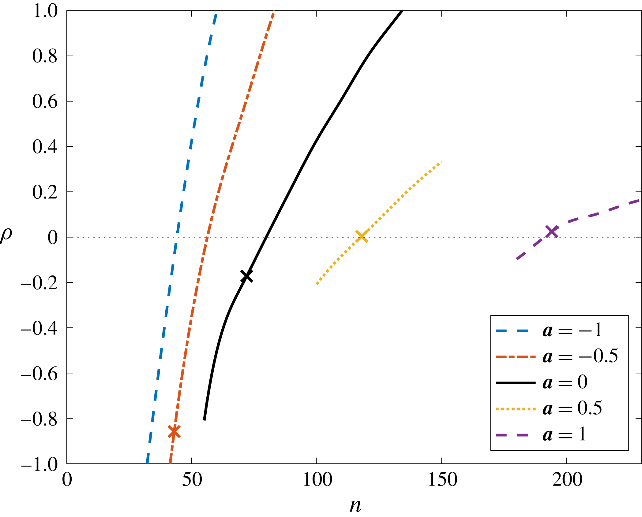
Results plotted in figure 10 are substituted into expression (4.7) for
 $\unicode[STIX]{x1D70C}$
that represents a measure of the long-term temporal growth. The solid black curve at the centre of figure 11 depicts the size of
 $\unicode[STIX]{x1D70C}$
against the matching value of
 $n$
. The cross symbol marks the location that
 $n=n_{a}\equiv 68$
. (The remaining four line types represent a similar set of calculations, but for the rotating-disc boundary layer with mass transfer. We will discuss these results in § 4.3.) A negative-valued
 $\unicode[STIX]{x1D70C}$
is obtained for
 $n=n_{a}\equiv 68$
and indeed
 $\unicode[STIX]{x1D70C}<0$
for all
 $n\lesssim 83$
. Thus, we might expect perturbations to this range of azimuthal mode numbers to display globally stable characteristics. For
 $n\gtrsim 83$
,
 $\unicode[STIX]{x1D70C}$
is positive, which indicates that globally unstable behaviour is established. On comparing these predictions for the global behaviour with the earlier numerical simulations of the genuine inhomogeneous flow (see figure 9), it would appear that our calculations based on coupling solutions of the homogeneous flow with the Ginzburg–Landau equation give a reasonable estimate for the onset of global instability. The results in figure 11 predict that
 $n_{c}\approx 83$
, which is within the parameter range
 $80\leqslant n\leqslant 100$
that numerical simulations suggest disturbances will become globally unstable.
Temporal growth rates
 $g_{i}$
for a disturbance centred about
 $r_{f}=521$
with
 $n=83$
(and
 $Re=521$
). Development in the genuine inhomogeneous flow at
 $r_{f}-50$
,
 $r_{f}-25$
,
 $r_{f}$
,
 $r_{f}+25$
and
 $r_{f}+50$
.

Figure 12 displays temporal growth rates established for a disturbance to the inhomogeneous flow with
 $n=83$
. The perturbation was impulsively excited about
 $r_{f}=521$
, which is near the radial location for critical absolute instability for this azimuthal mode number. Growth rates are plotted about the impulse centre and for four other radial positions. Temporal growth is found for
 $r\geqslant r_{f}$
, which appears to be tending towards positive constants for large time (at least for those plots centred about
 $r=r_{f}$
and
 $r_{f}+25$
). About those radial locations upstream of the impulse centre, growth rates are negative, but increasing. If the plots about
 $r=r_{f}-50$
and
 $r_{f}-25$
continue to grow along their current trajectories, unstable behaviour may be observed before the end of the second period of rotation. However, we are again unable to state with absolute certainty whether unstable characteristics will be sustained indefinitely. There is a possibility that growth rates will eventually reverse direction and tend towards negative values. Nevertheless, numerical calculations strongly suggest that there will at the very least exist a continuous time period for which disturbances are strongly unstable. This may then be sufficient to establish nonlinear effects and trigger full transition to turbulence.
4.3 Mass transfer effects
The above analysis was extended to include the effects of mass transfer through the disc surface. Two flows with injection (
 $\boldsymbol{a}<0$
) and two with suction (
 $\boldsymbol{a}>0$
) were considered, where the size of
 $\boldsymbol{a}$
(mass transfer coefficient) was the same as that implemented by Lingwood (Reference Lingwood1997a
) and Thomas & Davies (Reference Thomas and Davies2010). Numerical solutions of the homogeneous flow were simulated for a range of Reynolds numbers and azimuthal mode numbers. The parameters required for computing
 $\unicode[STIX]{x1D70C}$
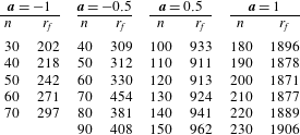
were then measured about the locations for critical absolute instability (as given in table 2). The corresponding
 $\unicode[STIX]{x1D70C}$
-solutions are plotted as a function of
 $n$
in figure 11, where
 $\boldsymbol{a}$
increases in size from left to right. Cross symbols on each data line mark the azimuthal mode number
 $n_{a}$
that is first to become absolutely unstable (refer to table 3). For those flows with
 $\boldsymbol{a}\leqslant 0$
,
 $\unicode[STIX]{x1D70C}$
is strongly negative for the critical mode number
 $n_{a}$
. Whereas for
 $\boldsymbol{a}>0$
,
 $\unicode[STIX]{x1D70C}$
is found to be near zero or marginally positive. Thus, our predictions based on the homogeneous flow would appear to reflect the original observations of Thomas & Davies (Reference Thomas and Davies2010) for disturbances
 $n=n_{a}$
; mass injection was shown to be stabilising, while mass suction promotes globally unstable characteristics.
Azimuthal mode number
 $n_{a}$
associated with the onset of absolute instability and the critical value
 $n_{c}$
for the appearance of globally unstable disturbances. The value
 $n_{c,H}$
is based on the predictions drawn by coupling the homogeneous flow calculations with the solutions of the Ginzburg–Landau equation, while
 $n_{c,I}$
represents the parameter range suggested by the numerical simulations of the inhomogeneous flow.

Temporal growth rates
 $g_{i}$
about the impulse centre for critical absolute instability. (a)
 $\boldsymbol{a}=-1$
; (b)
 $\boldsymbol{a}=-0.5$
; (c)
 $\boldsymbol{a}=0.5$
; (d)
 $\boldsymbol{a}=1$
. Parameter settings are as given in table 2.

For all of the flows considered in figure 11,
 $\unicode[STIX]{x1D70C}$
is positive for relatively high azimuthal mode numbers. Table 3 tabulates the predicted values for
 $n_{c}$
(labelled
 $n_{c,H}$
in the table) for each of the flows investigated. Figure 13 illustrates temporal growth rates for the four flows with mass transfer. Plots are depicted about the impulse centre that match the locations for critical absolute instability for each of the azimuthal mode numbers considered (refer to table 2 for the parameter settings). Some solutions could not be extended to the end of the time domain shown due to those numerical difficulties described earlier. For all flows considered, decreasing growth rates are obtained for sufficiently low azimuthal mode numbers. However, as
 $n$
increases to larger values, increasing and positive growth rates are established. Additionally, the variation of the temporal growth rate, that is measured from one azimuthal mode number to the next, changes far more rapidly for the flows with mass injection. For
 $\boldsymbol{a}=-1$
(figure 13
a) growth rates display relatively large variations between the lowest and highest mode numbers considered, whereas for
 $\boldsymbol{a}=1$
(figure 13
d) growth rates are clustered about a small region of the parameter space. This particular feature is consistent with the behaviour for
 $\unicode[STIX]{x1D70C}$
plotted in figure 11 that was found to vary far more quickly for negative
 $\boldsymbol{a}$
than for positive
 $\boldsymbol{a}$
.
Comparing those solutions given in figure 13 for the inhomogeneous flow with the predictions given by the Ginzburg–Landau modelling (figure 11 and table 3), suggests that the latter method can be used to give a reasonable estimate for the likely onset of global instability. For instance, growth rates in figure 13(a) (for
 $\boldsymbol{a}=-1$
) indicate that unstable behaviour arises for
 $n\in [40:50]$
, which coincides with the prediction that unstable disturbances develop for
 $n_{c}\approx 43$
. Similarly, in figure 13(c) (for
 $\boldsymbol{a}=0.5$
) calculations suggest that temporally growing perturbations first appear for
 $n\in [110:120]$
, while our predictive method suggests
 $n_{c}\approx 118$
.
5 Discussion
Results presented in the preceding sections are rather surprising, as the infinite rotating-disc boundary layer was previously thought to be globally stable to linear perturbations. However, there are some clues within the literature that maybe globally unstable characteristics should have been anticipated. Firstly, Thomas & Davies (Reference Thomas and Davies2010, Reference Thomas and Davies2013) found unstable behaviour comparable with that seen herein for the von Kármán flow, but with the inclusion of mass suction and an axial magnetic field. It was suggested (rather naively) that the locally stabilising effect brought about by the flow control mechanisms induced a form of global linear instability not previously seen on the infinite rotating-disc. Given the above observations it would appear that this original conclusion was incorrect and globally unstable behaviour should, for large enough azimuthal mode numbers, develop in many rotating boundary layers, comparable with that observed in other globally unstable flows (Huerre & Monkewitz Reference Huerre and Monkewitz1990). The primary goal of the earlier studies by Thomas and Davies was to examine the development of disturbances to the critical azimuthal mode number
 $n_{a}$
for absolute instability, and it was simply a coincidence that
 $n_{a}$
was large enough to establish global linear instability in those flows with mass transfer and an axial magnetic field.
A second indicator to the appearance of global linear instability relates to the local–global stability criteria described by Huerre & Monkewitz (Reference Huerre and Monkewitz1990). Local absolute instability is a necessary but not sufficient condition for the onset of globally unstable behaviour. The von Kármán flow is only absolutely unstable over a finite range for any fixed azimuthal mode number
 $n\geqslant 51$
, and for
 $n\lesssim 83$
this is not sufficient to generate global linear instability. However, for larger azimuthal mode numbers, disturbances triggered by an impulsive localised forcing exhibit globally unstable characteristics, that for the time duration numerical simulation results could be relied upon, is characterised by a faster than exponential temporal growth.
For the range of
 $n_{c}$
suggested as being necessary to establish global instability, critical Reynolds numbers for absolute instability are given as
 $516<Re_{a}<557$
, which coincides with the mid to upper range of values observed experimentally for the onset of transition. Thus, our simulation results may provide an explanation for why transition to turbulence in the rotating-disc boundary layer appears to be bounded by an upper Reynolds number limit.
Evidence for the appearance of the high azimuthal mode numbers in physical experiments is difficult to identify from within the available literature. Primarily this is because earlier studies examined convectively growing stationary cross-flow instabilities (Gregory et al.
Reference Gregory, Stuart and Walker1955), while more recently the focus has been aimed at connecting the initial appearance of absolute instability (
 $n=n_{a}$
) with the onset of transition. Additionally, it is possible that the physical interpretation of experimental results needs to be re-examined in light of the new findings. For instance, Imayama et al. (Reference Imayama, Alfredsson and Lingwood2012) undertook an experimental investigation of transition characteristics in the rotating-disc boundary layer. In their study growth rates were depicted using measurements of the root-mean-square as a function of the Reynolds number. In figure 5 of their paper a sharp exponential growth was observed about
 $475\leqslant Re\leqslant 530$
, while disturbances were shown to grow at a smaller exponential rate at larger
 $Re$
. Imayama et al. (Reference Imayama, Alfredsson and Lingwood2012) suggest that the change in slope near
 $Re=545$
could correspond to the appearance of a secondary instability to the global mode that is similar to that seen in an open rotating cavity (Viaud, Serre & Chomaz Reference Viaud, Serre and Chomaz2011). It was further suggested that the experimental observations may provide a validation for the theoretical predictions made by Pier (Reference Pier2003) that secondary instabilities to the primary instability are responsible for triggering transition. However, given the results of the current investigation, the change in growth observed by Imayama et al. (Reference Imayama, Alfredsson and Lingwood2012) might now be viewed as the emergence of the global linearly unstable high azimuthal mode numbers.
5.1 Strong amplification of convective instabilities
The apparent lack of evidence for the high
 $n$
mode numbers in experiments might be explained by considering the huge growth associated with the disturbance maxima of the lower-valued azimuthal mode numbers. Figures 4 and 7 demonstrate that perturbations can grow by several
 $N$
-factors (recall equation (3.2)) over a very short radial range. Indeed Davies & Carpenter (Reference Davies and Carpenter2003) show that disturbances grow by many orders of magnitude in only one period of the disc rotation (see figure 9 of their paper). To illustrate the considerable growth of the wavepacket maxima, many disturbances were simulated for initial settings (and a comprehensive range of
 $n$
) that match the experimental conditions implemented by Lingwood (Reference Lingwood1995) and Othman & Corke (Reference Othman and Corke2006).
Spatial and temporal development of the azimuthal vorticity on the disc surface
 $|\unicode[STIX]{x1D714}_{\unicode[STIX]{x1D703},w}|$
, for impulsively excited disturbances centred about
 $r_{f}=311$
. (a)
 $n=50$
; (b)
 $n=75$
; (c)
 $n=100$
. Magnitudes
 $|\unicode[STIX]{x1D714}_{\unicode[STIX]{x1D703},w}|$
have been normalised so that all perturbations are equal to unity at
 $t/T=0.2$
.

Numerical simulations were impulsively excited about
 $r_{f}=311$
for
 $n\in [5:150]$
at regular intervals
 $\unicode[STIX]{x0394}n=5$
. A similar analysis was undertaken by Davies & Carpenter (Reference Davies and Carpenter2003) for
 $n=67$
(see figure 19 of their study). Figure 14 depicts the development of three spatial–temporal wavepackets established for
 $n=50$
,
 $75$
and
 $100$
. Contours are again labelled using a logarithmic
 $N$
-factor, while perturbations have been normalised about
 $t/T=0.2$
. (It should be noted that the leading and trailing edge contours are not represented by the same
 $N$
-factor, as the three disturbances develop at varying rates and only grow in magnitude once they have attained radial positions that match the onset of convective or absolute instability associated with that particular azimuthal mode number.) The trailing edge of the disturbance wavepacket given for
 $n=50$
(illustrated in figure 14
a) displays convective characteristics and propagates downstream along the radial direction, while the trailing edge established for the largest azimuthal mode number (plotted in figure 14
c) would appear to be slowing down as it approaches the radial range
 $500<r<600$
. Based on the results presented in § 3 it might be speculated that the trailing edge of the latter perturbation will, given sufficient time, reverse direction and propagate radially upstream.
Contours of the wavepacket maxima,
 $N_{max}$
, in the
 $\{t/T,n\}$
-parameter space for disturbances impulsively excited about
 $r_{f}=311$
. Magnitudes
 $|\unicode[STIX]{x1D714}_{\unicode[STIX]{x1D703},w}|$
have been normalised so that all perturbations are equal to unity at
 $t/T=0.2$
and the dashed line illustrates the development of the most amplified azimuthal mode number.

Although the disturbance presented for
 $n=50$
displays convectively unstable behaviour, its maximum amplitude grows at a faster rate than that established for the two higher-valued azimuthal mode numbers. For instance, contour levels labelled
 $N=2$
are first obtained about
 $r\approx 400$
for
 $n=50$
, but are not achieved until
 $r\approx 470$
and
 $590$
for
 $n=75$
and
 $100$
, respectively. Furthermore, about
 $r=500$
, the smaller azimuthal modal disturbance has a magnitude of order
 $N=7$
, which is significantly greater than the corresponding amplification factors
 $N=3$
and
 $-5$
obtained for the larger-valued
 $n$
.
The wavepacket maximum
 $$\begin{eqnarray}\displaystyle N_{max}=\max _{r}(N) & & \displaystyle\end{eqnarray}$$
is computed for all disturbances
 $n\in [5:5:150]$
and is plotted in figure 15 using contours in the
 $\{t/T,n\}$
-plane. Contours are plotted at five-step intervals and the dashed curve depicts the path of the most amplified mode. Convective modes
 $n<51$
are shown to achieve the greatest amplification factors and absolutely unstable modes (
 $n\geqslant 51$
) only attain comparable amplitudes at later points in time. Using an
 $\text{e}^{N}$
method for predicting transition in wind-tunnel tests on airfoils, Van Ingen (Reference Van Ingen1956) and Smith & Gamberoni (Reference Smith and Gamberoni1956) found the onset of transition coincides with an
 $N$
-factor between 7 and 9. Although the
 $\text{e}^{N}$
method does not account for receptivity effects or nonlinear mechanisms it is still today the primary tool for transition prediction in the aerospace industry. Supposing that we can utilise this particular strategy for determining the onset of transition in the infinite rotating-disc boundary layer, figure 15 would suggest that convectively unstable modes quickly achieve large enough magnitudes to trigger nonlinearity and the latter stages of the laminar–turbulent transition process (assuming of course that a similarly sized
 $N$
-factor, as that predicted by Van Ingen Reference Van Ingen1956, is required to establish transition on the rotating-disc). Figure 16 displays
 $N$
-factors in the
 $\{t/T,n\}$
-plane about
 $r=400$
,
 $500$
,
 $550$
and
 $600$
, where
 $N_{max}$
is respectively of the order 1, 7, 11 and 15, with the most amplified azimuthal mode number corresponding to
 $n=45$
, 50, 50 and 55. Hence, convective disturbances attain very large magnitudes
 $N\in [7:11]$
over the radial range
 $500\leqslant r\leqslant 550$
, which matches the onset of experimentally observed transition. Thus, larger
 $n$
-modes may not be strongly relevant to the long-term disturbance development; smaller
 $n$
-modes can achieve very large magnitudes that might be sufficient to trigger nonlinearity and transition, before the high
 $n$
-modes develop further outboard.
Contours of
 $N=\ln |\unicode[STIX]{x1D714}_{\unicode[STIX]{x1D703},w}|$
in the
 $\{t/T,n\}$
-parameter space about fixed radial locations
 $r$
, for disturbances impulsively excited about
 $r_{f}=311$
. (a)
 $r=400$
; (b)
 $r=500$
; (c)
 $r=550$
; (d)
 $r=600$
.

6 Conclusions
An investigation has been carried out on the global linear stability of the von Kármán flow on an infinite rotating-disc boundary layer, for an extensive range of azimuthal mode numbers
 $n$
. This study expands upon earlier investigations (Davies & Carpenter Reference Davies and Carpenter2003) that found globally stable characteristics for azimuthal mode numbers near the onset of absolute instability. For larger azimuthal mode numbers, disturbances excited by an impulsive forcing display a rapidly increasing temporal growth that is similar to that found when mass suction was applied through the disc surface (Thomas & Davies Reference Thomas and Davies2010). Numerical simulations suggest that a change in the global response arises for
 $n\in [80:100]$
that corresponds to the mid–upper range of Reynolds numbers reported experimentally for the onset of transition. Thus, the absolutely unstable mechanism establishes a form of global instability that comprises a faster than exponential temporal growth, but only for azimuthal mode numbers greater than the conditions for critical absolute instability. However, as with previous studies pertaining to the global linear stability of the infinite rotating-disc, there was no selection of any global temporal frequency, which might have been expected for a globally unstable flow. Instead temporal frequencies varied with both the radial location and time, at least for the time duration that numerical simulations could be accurately computed. As mentioned above, extending simulations of disturbance development beyond that illustrated herein was very difficult to accomplish due to the huge amplitudes that perturbations could achieve.
Comparisons were drawn with solutions of the Ginzburg–Landau equation with a linearly varying stability parameter (Hunt & Crighton Reference Hunt and Crighton1991), using a technique similar to that implemented by Davies et al. (Reference Davies, Thomas and Carpenter2007) and Thomas & Davies (Reference Thomas and Davies2010, Reference Thomas and Davies2013). However, whilst Davies and co-workers based their Ginzburg–Landau modelling on solutions of the genuine radially dependent flow, the analysis conducted herein utilised results of the homogeneous flow. Computations predict that globally unstable behaviour can be achieved for azimuthal mode numbers
 $n\gtrsim 83$
, which is in reasonably good agreement with numerical solutions of disturbance development to the inhomogeneous flow. Results show that the radial variations in the temporal growth rate increases for larger
 $n$
and are eventually large enough to engineer globally unstable characteristics.
The study was extended to include mass transfer through the disc surface. For those flows considered, both numerical simulations and Ginzburg–Landau modelling displayed strong temporal growth for relatively high azimuthal mode numbers. Hence, it would appear that the behaviour seen here for the von Kármán flow is a consistent feature of rotating boundary layers. Furthermore, we anticipate that globally unstable disturbances will be found in many other rotating boundary layers, including, but not limited to, the Bödewadt–Ekman–Kármán family of flows, rotating-spheres and rotating-cones (Lingwood Reference Lingwood1997b ; Garrett & Peake Reference Garrett and Peake2002, Reference Garrett and Peake2007).
Although a form of global instability can develop for sufficiently large azimuthal mode numbers, our analysis suggests that transition to turbulence may still be dominated by the huge spatial growth associated with convective instabilities. The amplitude of disturbances, at relatively small azimuthal mode numbers, increases in size very quickly and achieves exponential orders of magnitude
 $N\in [7:11]$
across the range of Reynolds numbers (radii) that transition is observed experimentally. Similar amplitudes are only achieved by the absolutely unstable modes at larger radii and at later points in time. Hence, the globally unstable high
 $n$
-modes are unlikely to establish themselves over a sufficient radial range before nonlinear effects are triggered by the faster growing convective instabilities.
Diagram illustrating the local and global stability of the rotating-disc boundary layer.
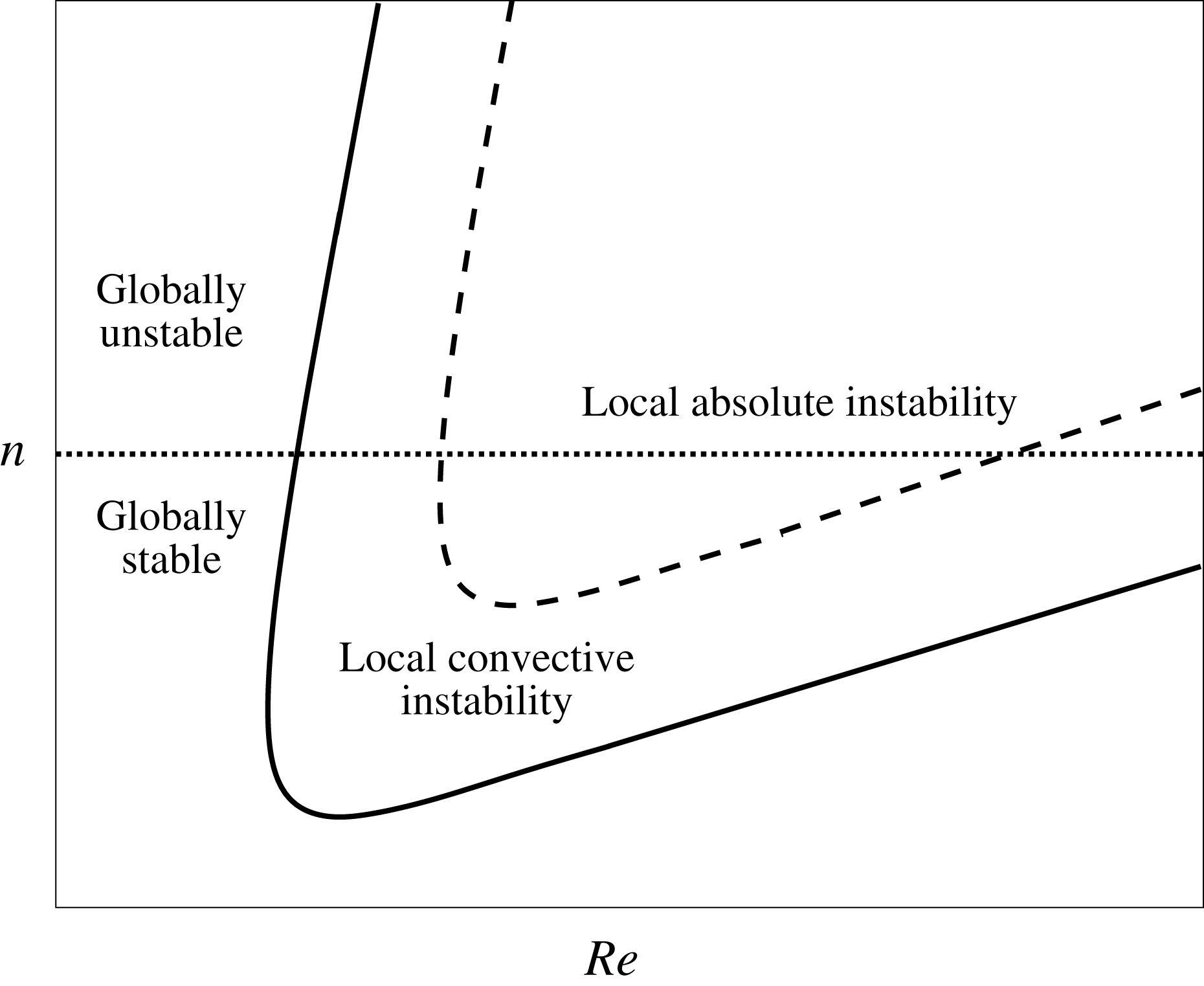
Results of our investigation suggest that the local–global linear stability of the infinite rotating-disc boundary layer (and similar flows) can be described by the
 $\{Re,n\}$
-diagram illustrated in figure 17. For small
 $Re$
and
 $n$
, the flow is stable. Then as
 $Re$
and
 $n$
are increased to larger values, regions of local convective (solid curve) and absolute (dashed) instability emerge. The flow is then globally stable up to some critical mode number
 $n_{c}$
(represented by the horizontal dotted line), even though the flow might be locally absolutely unstable for a finite range of
 $Re$
. However, for
 $n>n_{c}$
(which is not necessarily equal to
 $n_{a}$
) globally unstable characteristics emerge. Improvements to the prediction for
 $n_{c}$
and the local–global stability diagram might be achieved by implementing the Hunt & Crighton (Reference Hunt and Crighton1991) Ginzburg–Landau model with a quadratically varying stability parameter, with global stability determined using the saddle point criteria described in Huerre & Monkewitz (Reference Huerre and Monkewitz1990).
Finally, it should be emphasised that our results do not invalidate the recent theory and experiments that suggest global instability can be engineered at smaller azimuthal mode numbers by modelling a radially finite rotating-disc. Furthermore, results of this investigation pose a number of questions for the future study of rotating-discs. Do high azimuthal mode numbers affect stability and transition processes on finite discs (Healey Reference Healey2010; Imayama et al. Reference Imayama, Alfredsson and Lingwood2013; Pier Reference Pier2013; Appelquist et al. Reference Appelquist, Schlatter, Alfredsson and Lingwood2015a ,Reference Appelquist, Schlatter, Alfredsson and Lingwood b , Reference Appelquist, Schlatter, Alfredsson and Lingwood2016) and do they impact the formation of secondary instabilities (Pier Reference Pier2003, Reference Pier2007)?



