1. Introduction
The Amazon is the world's largest rainforest, stretching over an area of more than five million km2. In Brazil, the forest originally occupied over 4 million km2 – an area equivalent to almost half of continental Europe. Today, around 80 per cent of the Brazilian Amazon remains covered by native vegetation, making it an important carbon sink. Moreover, the Brazilian Amazon holds unique biodiversity and 20 per cent of the planet's fresh water (MMA, 2012). Protecting the Amazon from illegal deforestation and enforcing environmental regulation in the region is a challenge as immense as the forest itself. Yet, the pace of forest clearings appears to have lost momentum in recent years. Amazon deforestation rates escalated in the early 2000s, but after peaking at over 27, 000 km2 in 2004, decreased sharply to about 5, 000 km2 in 2011 (INPE, 2013).
In 2008, the Brazilian Ministry of Environment blacklisted 36 municipalities to better target monitoring and law enforcement efforts, setting them as Municípios Prioritários (Priority Municipalities, or MPs). This group of municipalities accounted for 45 per cent of the Amazonian deforestation in the previous year, an astonishing figure considering that Brazil has 547 municipalities that transect the Biome. Seven municipalities were added in 2009 and another seven were included in 2011. The MPs were intended to serve as targets for a more stringent system of deforestation monitoring and environmental law enforcement. The Brazilian Institute for the Environment and Renewable Natural Resources (Ibama), which operates as the national environmental police and law enforcement authority, focused law enforcement activities on MPs, issuing fines and embargoing farms. These command-and-control activities were complemented by a series of actions that were not explicit in the original decree launched by the government. These actions included political commitments led by local governments, changes in the approval of subsidized credit contracts, the refusal of meatpacking plants to buy cattle from embargoed farms and development of local plans for sustainable production (Brito et al., Reference Brito, Souza and Amaral2010; Maia et al., Reference Maia, Hargrave, Gómez and Röper2011; Arima et al., Reference Arima, Barreto, Araújo and Soares-Filho2014).
Was the MPs policy effective in curbing deforestation? What is the relative importance of the monitoring and law enforcement activities in comparison to the other actions? Was agricultural production affected in those municipalities?
We address these questions in a panel of municipalities in the Brazilian Amazon from 2002 through 2011. Deforestation data is obtained from processed satellite imagery made publicly available by the National Institute for Space Research. Based on the decrees enacted by the government, we create a dummy variable indicating which municipalities are blacklisted in each year. We run fixed-effect models using the blacklist dummy as the main variable of interest.
Our results indicate that the MPs policy significantly reduced deforestation. According to our estimates, the policy avoided the clearing of 11, 218 km2 of forest area from 2008 through 2011. In the absence of the policy, the deforestation would have been 54 per cent higher than the 20, 689 km2 observed for the period. In a robustness exercise, we show that there is no deforestation pre-trend that systematically differentiated municipalities before they became blacklisted. We also show that even controlling for interactions of different characteristics (such as poverty, per capita GDP, protected areas, soybean planted area, head of cattle per km2, etc.) with a linear time trend, the effect does not change. Changes in protected areas and other observed variables in the neighbour municipalities do not affect the results either.
After identifying the overall impact of the MPs policy, we study the relative importance of the monitoring and law enforcement in comparison to other political and economic actions that came along. While we find that the number of fines increased in the blacklisted municipalities, there was no effect on agricultural GDP, crop production, or credit concessions (total, crops and livestock). This result suggests that the command-and-control component was the primary driver of the deforestation slowdown determined by the policy. Moreover, it suggests that combatting deforestation in the Brazilian Amazon does not necessarily create obstacles for agricultural production.
In order to further explore this issue, we come back to the impact of MPs on deforestation and check what happens when we control for the number of fines. The challenge in this exercise is that the number of fines is endogenously determined. We use an instrumental variable approach, based on Assunção et al. (Reference Assunção, Gandour and Rocha2013), in which cloud cover is used as a source of exogenous variation in the number of fines. The main idea is that, after 2004, the government uses satellite imagery to monitor and allocate law enforcers. But the technology does not identify deforestation hot spots under clouds, which generates exogenous variation in law enforcers and, therefore, on the number of fines. When adequately controlling for the number of fines, the effect of the MPs on deforestation disappears.
There are a few recent papers on the impact of blacklisting on deforestation in the Amazon. Arima et al. (Reference Arima, Barreto, Araújo and Soares-Filho2014); Cisneros et al. (Reference Cisneros, Zhou and Börner2015), using different approaches, find significant impacts of the policy on deforestation rates. The estimated magnitudes vary across studies as they use different methods. Our results are quantitatively similar to the ones reported in Arima et al. (Reference Arima, Barreto, Araújo and Soares-Filho2014). Sills et al. (Reference Sills, Herrera, Kirkpatrick, Brandão, Dickson, Hall, Pattanayak, Shoch, Vedoveto, Young and Pfaff2015) examine the case of the Paragominas municipality, where the local government put additional effort into creating a local program to combat deforestation. They show that Paragominas has reduced deforestation more than the other MPs, suggesting that the complementary actions have contributed to the policy impact.
Our study contributes to this literature by assessing in more detail the mechanisms through which the policy has affected deforestation. We take two additional steps compared to the literature. First, we measure the direct effect of MPs on applied fines, credit and agricultural production, showing that the policy only impacts positively the number of fines (with no effect on credit or agricultural production). Second, we follow the approach of Assunção et al. (Reference Assunção, Gandour and Rocha2013) to adequately control for the number of fines, showing that the stricter monitoring implied by the policy is the main driver behind its impact on deforestation. The results are in line with the literature that shows local inspections effectively reducing deforestation in the states of Pará and Mato Grosso (Börner et al., Reference Börner, Kis-Katos, Hargrave and König2015).
Deforestation is also affected by some structural determinants such as population, road density, and agroclimatic characteristics (Reis and Margulis, Reference Reis, Margulis, Dornbusch and Poterba1991; Reis and Guzmán, Reference Reis, Guzmán, Brown and Pearce1994; Pfaff, Reference Pfaff1999; Chomitz and Thomas, Reference Chomitz and Thomas2003). Recently, many authors have shown that how the policies interact with each other and with other determinants matters (Pfaff et al., Reference Pfaff, Robalino, Walker, Aldrich, Caldas, Reis, Perz, Bohrer, Arima and Laurance2007, Reference Pfaff, Robalino, Herrera and Sandoval2015; Herrera, Reference Herrera2015; Robalino et al., Reference Robalino, Pfaff and Villalobos2015). We show that even after controlling for some of these variables, the interaction between them and a linear time-trend, and the value of these variables in MPs' neighbours, MPs played an important role in reducin deforestation in the Amazon through the monitoring mechanism.
More recently, there is a literature on the immediate drivers of the recent Amazon deforestation slowdown. Assunção et al. (Reference Assunção, Gandour and Rocha2012) show that, even when controlling for commodity prices and relevant fixed effects, conservation policies introduced in the second half of the 2000s helped avoid over 60, 000 km2 of forest clearings. Hargrave and Kis-Katos (Reference Hargrave and Kis-Katos2013) and Assunção et al. (Reference Assunção, Gandour and Rocha2013) find a negative relationship between the number of fines and deforestation in the Amazon. We contribute to this particular literature showing that targeting can further boost effective monitoring and law enforcement efforts.
The paper is also related to a broader literature on the evaluation of effectiveness of environmental monitoring and law enforcement. Gray and Shimshack (Reference Gray and Shimshack2011) provide a recent survey of this literature. Most studies refer to plant-level environmental performance, as captured by standard emissions or accidental discharges (see, for example, Epple and Visscher, Reference Epple and Visscher1984; Magat and Viscusi, Reference Magat and Viscusi1990; Anderson and Talley, Reference Anderson and Talley1995; Eckert, Reference Eckert2004; Gray and Shadbegian, Reference Gray and Shadbegian2005; Shimshack and Ward, Reference Shimshack and Ward2005; Earnhart and Segerson, Reference Earnhart and Segerson2012). Our paper addresses a different dimension of environmental monitoring and law enforcement, focusing on the impact of a targeted law enforcement policy on deforestation.
Finally, this paper contributes to the ongoing debate about the relationship between economic growth and the environment (Grossman and Krueger, Reference Grossman and Krueger1995; Arrow et al., Reference Arrow, Bolin, Costanza, Dasgupta, Folke, Holling, Jansson, Levin, Maler, Perrings and Pimentel1996). There is an extensive literature addressing the question about the relationship between income and forest conservation. Cropper and Griffiths (Reference Cropper and Griffiths1994) and Panayotou (Reference Panayotou, Ahmed and Doeleman1995) find no significant relationship between the two, while Antle and Heidebrink (Reference Antle and Heidebrink1995) document a positive relationship between afforestation and income, but only for income levels above a certain threshold. Foster and Rosenzweig (Reference Foster and Rosenzweig2003) provide evidence of there being no relationship between forest cover and economic growth in open economies, but a positive relationship in closed ones. Our results show that it is possible to reduce deforestation without constraining total agricultural production. Facing more effective monitoring, farmers may shift away from land-intensive practices towards higher yield agriculture. In this context, productivity gains can explain the reduction in deforestation without a meaningful impact on agricultural production.
The rest of this paper is organized as follows. Section 2 discusses the institutional context in the time of the implementation of MPs. Section 3 provides a detailed description of the data used in the paper. Section 4 explains the empirical strategy used to calculate the impact of MPs on deforestation. Section 5 discusses the results of the paper and section 6 addresses the conclusions and policy implications of our results.
2. Institutional context
Brazilian conservation policies were reformulated twice during the 2000s. The first change was made in 2004, when satellite imagery and other efforts strengthened monitoring and law enforcement in the Amazon. The second change began in 2008 and was comprised of better targeting of the protection policies through a blacklist of MPs. These two turning points in the Brazilian conservation policies are analyzed in Assunção et al. (Reference Assunção, Gandour and Rocha2012).
2.1 Phase I: Strengthened monitoring and law enforcement
The government launched, in 2004, a new approach to combat deforestation in the Brazilian Amazon after a surge in the deforestation rates in the early 2000s. The pivotal conservation policy effort was the Action Plan for the Prevention and Control of Deforestation in the Legal Amazon (Plano de Preven ção e Controle do Desmatamento na Amazônia Legal, or PPCDAm). The PPCDAm integrated actions across different government institutions and proposed new procedures for monitoring, environmental control, and territorial management. PPCDAm also improved the qualifications of the environmental authority personnel through intensive training and recruitment.
One of the key components of PPCDAm was the remote sensing-based Amazon monitoring capacity brought about by the implementation of the satellite-based Real-Time Detection of Deforestation System (DETER) – the main tool for allocating law enforcement efforts in the Amazon. Developed by the National Institute for Space Research, DETER is a satellite-based system that captures and processes imagery on Brazilian Amazon forest cover in 15-day intervals, with precision of 25 hectares. The imagery is translated into digital maps, which are used to locate deforestation hot spots and issue alerts signaling areas in need of attention.
Before the DETER system, the Amazon monitoring was dependent on voluntary and anonymous reports of threatened areas. With the new system, the environmental authority was given rapid access to geo-located data on forest clearing activity and was thus able to better identify and more quickly act against illegal deforestation.
This change was important because a part of deforestation activities has taken place on lands that were not public registered, making enforcement more difficult. Therefore, it is very important for law enforcers to act while deforestation is happening. Otherwise, it is hard to identify law offenders and impose penalties. When the federal police, Ibama and/or other police agents identify illegal activities in real time, they are able to impose sanctions, destroying equipment, seizing the illegal wood, applying fines, and embargoing areas for credit.
There is a specific characteristic of the DETER system that we also explore in this paper, following Assunção et al. (Reference Assunção, Gandour and Rocha2013). The system is not able to identify land cover patterns beneath clouds. Cloud coverage, which can be quite extensive in the Amazon, limits the ability of the environmental authority to identify deforestation hot spots and, thus, is an exogenous source of variation in monitoring and law enforcement. Assunção et al. (Reference Assunção, Gandour and Rocha2013) explore this characteristic to estimate the impact of monitoring and law enforcement on deforestation. This paper uses a similar method.
2.2 Phase II: Better targeting
The creation of a blacklist to better target efforts that combat illegal deforestation was the main component of the second phase of the PPCDAm. The signing of Presidential Decree 6,321 in December 2007 established the legal basis for singling out municipalities with intense deforestation activity and taking differentiated action towards them. These municipalities, classified based on their recent deforestation history, were marked as in need of priority action to prevent, monitor and combat illegal deforestation. Any Legal Amazon municipality could be added to what became known as the list of Municípios Prioritários (MPs). Municipality-level selection criteria for this list were: (i) total deforested area; (ii) total deforested area over the past three years; and (iii) increase in the deforestation rate in at least three of the past five years. Exiting the list of MPs was conditioned upon significantly reducing deforestation. Issued in January 2008, MMA Ordinance 28 listed the first 36 MPs. Seven municipalities were added to the list in 2009, and another seven in 2011.
Differential action taken in MPs largely consisted of more rigorous environmental monitoring and law enforcement. Ibama monitored the municipalities more closely and dedicated a larger share of its resources to them. Licensing and georeferencing requirements for rural establishments were harsher in MPs, and, in an effort to identify fraudulent documents and illegal occupations, private land titles were revised.
In addition to concentrating a large share of Ibama's attention and monitoring efforts, MPs also became subject to a series of other administrative measures that did not necessarily stem from command-and-control policy. Although not officially established through legislation, these measures imposed an additional cost to being blacklisted. These actions have included political commitments led by local governments, changes in the approval of subsidized credit contracts, the refusal of meatpacking plants to buy cattle from embargoed farms, and development of local plans for sustainable production (Brito et al., Reference Brito, Souza and Amaral2010; Maia et al., Reference Maia, Hargrave, Gómez and Röper2011; Arima et al., Reference Arima, Barreto, Araújo and Soares-Filho2014).
In light of this, the impact of being added to the list of MPs could be broader than just that of being subject to stricter monitoring and law enforcement. Our empirical analysis takes this potentially broader impact into consideration.
A closer look at the example of the Paragominas, a municipality in the State of Pará, can provide a more concrete notion of what happened. Paragominas was founded in 1965 as part of the occupation process that followed the construction of the Belem-Brasilia road. Logging and extensive practices in agricultural and cattle ranching have resulted in a suppression of 45 per cent of the original forested area.
Paragominas was in the MPs list published in 2008 and was the first municipality to be removed from the list, after reducing deforestation dramatically, in 2013. Right after being included in the MPs list, Paragominas started a process to set up a plan to reduce deforestation, led by the local government. According to Brito et al. (Reference Brito, Souza and Amaral2010), the mayor's office, local producers associations, and groups from the civil society signed a pact for zero deforestation. Under the new regime, the mayor's office started to support the monitoring and law enforcement implemented by the federal government, while the producers associations with support from NGOs organized a series of meetings and seminars to promote registry and titling, in order to improve property rights. As a consequence, the deforestation rate computed by the PRODES system was reduced from 64.1 km2 in 2007/2008 to 18.2 km2 in 2011/2012.
3. Data
We compile data from different sources.
3.1 Deforestation
Data on deforestation is built from satellite-based images that are processed at the municipality level and publicly released by PRODES/INPE. We define deforestation as the annual deforestation increment, that is, the area in square kilometers of forest cleared over the twelve months leading up to August of a given year.Footnote 1
For any given municipality, cloud cover during the period of remote sensing may compromise the accuracy of satellite images, requiring images to be produced at a different time. As a result, image records for different years may span from less than to more than twelve months. To control for measurement error, variables indicating unobservable areas are included in all regressions. This data is also publicly available at the municipality-by-year level from PRODES/INPE.
To smoothen the cross-sectional variation in deforestation that arises from municipality size heterogeneity, we use a normalized measure of the annual deforestation increment as in (Assunção et al., Reference Assunção, Gandour and Rocha2012, Reference Assunção, Gandour and Rocha2013). The normalization ensures that our analysis considers relative variations in deforestation increments within municipalities. The variable is constructed according to the following expression:
 $$Deforest_{it}=\displaystyle{{ADI_{it}-{\overline{ADI}}_{it}}\over{sd\left(ADI_{it}\right)}},$$
where Deforest it is the normalized annual deforestation increment for municipality i and year t; ADI it is the annual deforestation increment measured in municipality i between 1 August of t−1 and 31 July of t; and  $\overline {ADI}_{it}$ and sd(ADI it) are, respectively, the mean and the standard deviation of the annual deforestation increment calculated for each i over the 2002 through 2011 period. The variable ADI it replaces Deforest it in robustness checks. Our sample does not include municipalities that showed no variation in deforestation throughout the sample years, as this variation is needed to calculate the normalized variable.
3.2 Municípios Prioritários (MPs)
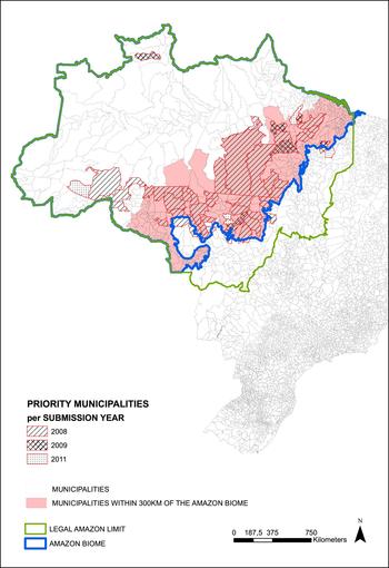
Our main interest is to study the effect of blacklisting a municipality on different economic outcomes. Thus, we define a variable MP it that is set to 1 if municipality i is in the list in year t and 0 otherwise. Figure 1 shows the location of the municipalities that were included in the lists of 2008, 2009 and 2011. We can see that, except for a few cases, they are concentrated in the southern and eastern parts of the Amazon, less than 300 km from the Amazon Biome border.
Blacklisted municipalities. Source: IBGE and Ministry of Environment.

3.3 Number of fines
We use the total number of fines applied as sanctions for environmental crimes in each municipality as a measure of the intensity of monitoring and law enforcement at the municipality level. We also normalize the number of fines in the same way we did to deforestation data. The data are publicly available from Ibama.
It is worth highlighting that the knowingly low collection rates for environmental fines applied in Amazon municipalities do not interfere with our analysis (Hirakuri, Reference Hirakuri2003; Brito and Barreto, Reference Brito and Barreto2008; Brito, Reference Brito2009). These fines are often accompanied by other sanctioning instruments that are more binding, such as seizure and destruction of production goods, tools and materials, and embargoes of production areas. Because panel data for the use of these instruments are not available, we use the number of fines as a proxy for command-and-control efforts as a whole. Essentially, we are interested in exploring fines as a means of capturing the effect of environmental police (Ibama) presence – not of the sanctioning instrument itself – on deforestation.
To maintain consistency across our panel data, we consider the PRODES year – 1 August t−1 through 31 July t – as the relevant unit of time in our sample. Thus, for each municipality, the total number of fines in a given year captures all fines applied in that municipality in the twelve months leading up to August of that year.
3.4 Credit and agricultural production
The credit data is constructed from a contract-level microdata set of rural credit loan contracts compiled by the Central Bank from Recor data from 2003 to 2011. This is an administrative microdata set encompassing all rural contract records negotiated by official banks – both public and private – and credit cooperatives in the Legal Amazon. It contains detailed information about each contract, such as the exact day on which it was signed, its value in Brazilian real (BRL), the contracted interest rate and maturation date, its intended use by agricultural activity, and the category under which credit was loaned (short-term operating funds, investment or commercialization). All contracts are linked to a code identifying the municipality in which the borrower's landholding is located. We add up the value of the contract loans across all days in each year and each municipality to convert the microdata panel into a municipality-by-year panel.
To smooth the large cross-sectional variation in values of credit contracts generated by different municipality sizes, we use a normalized measure of rural credit. This normalization ensures that our analysis captures relative variations in credit lending within municipalities. The variable is constructed according to the following expression:
 $$ Credit_{it}=\displaystyle{{C_{it}-\overline{C}_{it}}\over{sd\left( C_{it}\right)}},$$
where Credit it is the normalized amount of rural credit loaned in municipality i and year t; the term C it is the amount of rural credit loaned in municipality i and year t in BRL; and the terms  $\overline {C}_{it}$ and sd(C it) are, respectively, the mean and the standard deviation of the amount of rural credit loaned in municipality i over the 2003–2011 period.
We also have data from national accounts (IBGE) on agricultural GDP (which includes crop and livestock production) from 2002 to 2009. Besides that, we have data from the Monthly Crop Survey (PAM/IBGE) on crop production from 2002 to 2011.
3.5 Cloud coverage
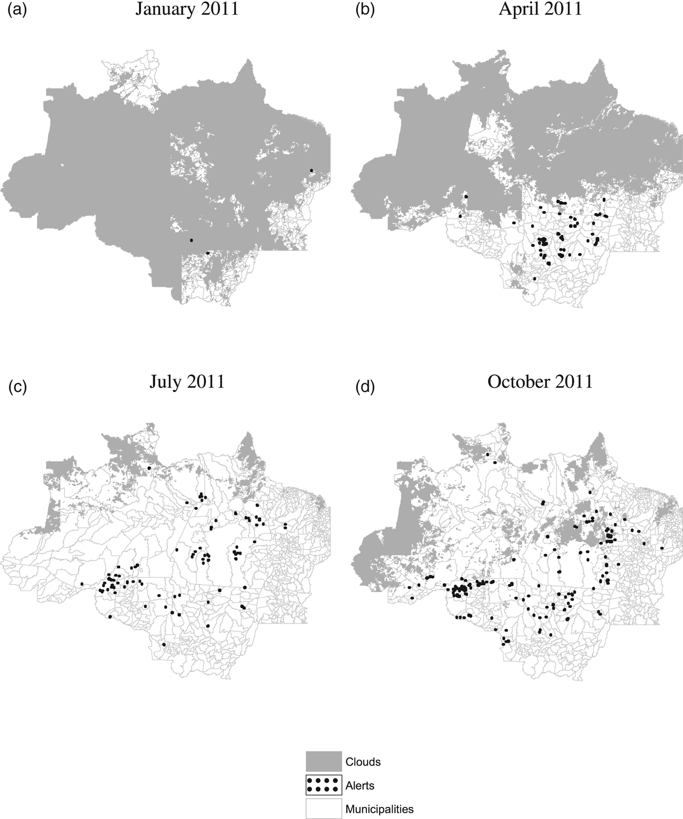
Georeferenced data on deforestation activity produced by the satellite-based DETER system are used to identify deforestation hot spots and issue alerts that serve to target law enforcement activity. Figure 2 shows examples of maps containing both cloud coverage and alerts captured by DETER. In addition to portraying the high degree of within-year variation in DETER cloud coverage, figure 2 also clearly illustrates DETER's inability to detect land cover patterns in areas covered by clouds – typically, no deforestation activity is captured and no deforestation alerts are issued in these areas. This supports the perception that the allocation of Ibama personnel is directly affected by DETER cloud coverage, such that law enforcers are less likely to be present in areas that are systematically under greater cloud coverage.
DETER cloud coverage and deforestation alerts. (a) January 2011 (b) April 2011 (c) July 2011 (d) October 2011.

We are, then, interested in exploring how DETER cloud coverage affects Ibama presence in the Amazon. To do this, we use georeferenced data from DETER/INPE that map cloud coverage over the Amazon throughout the year. When visibility is at least partial, these maps show exactly which areas were covered by clouds (see figure 2). When visibility is too precarious to derive information about land cover, however, no map is produced – we assume DETER cloud coverage to be complete in this case. We use the 15-day periodical data to calculate, for each sample municipality and year, average DETER cloud coverage for that municipality and year both in absolute (square kilometers) and relative (share of total municipality area) terms. Again, the relevant unit of time is the PRODES year. We use this constructed variable as an instrument for the number of fines applied to each Amazon municipality.
3.6 Agricultural output prices
Agricultural prices are endogenous to local agricultural production. Thus, to control for fluctuations pressuring deforestation at the municipality level, we must construct output price series that capture exogenous variations in the demand for agricultural commodities produced locally. As argued in Assunção et al. (Reference Assunção, Gandour and Rocha2012), agricultural commodity prices recorded in the southern Brazilian state of Paraná are highly correlated with average local crop prices calculated for the Legal Amazon sample municipalities. Hence, we use the Paraná agricultural commodity price series as exogenous indicators of local market conditions within our empirical context. Prices for beef cattle, soybean, cassava, rice, corn and sugarcane were collected at the Agriculture and Supply Secretariat of the State of Paraná (Secretaria de Agricultura e do Abastecimento do Estado do Paraná, or SEAB-PR). Soybean, cassava, rice and corn are predominant crops in the Legal Amazon in terms of harvested area. Although not a predominant crop in the region, sugarcane is also included to take into consideration the recent expansion of Brazilian ethanol biofuel production. Together, the five crops account for approximately 70 per cent of total harvested area averaged across sample years.
The Paraná price series are used to build two variables of interest. The first of these variables, an annual index of crop prices, is constructed in three steps. First, we calculate nominal monthly price series for each calendar year-month and culture. Annual prices are deflated to year 2011 BRL and are expressed as an index with base year 2011.
Second, we calculate a weighted real price for each of the crops according to the following expression:
 $$PPA_{itc}=PP_{tc}\ast {A}_{ic,2000-2001},$$
where PPA itc is the weighted real price of crop c in municipality i and year t; PP tc is the Paraná-based real price of crop c in year t expressed as an index with base year 2000; and A ic,2000−2001 is the share of municipal area used as farmland for production of crop c in municipality i averaged over the 2000 through 2001 period.Footnote 2 This latter term captures the relative importance of crop c within municipality i's agricultural production in the years immediately preceding the sample periods. It thus serves as a municipality-specific weight that introduces cross-sectional variation in the commodity price series.
Third, we use principal component analysis on the weighted real crop prices to derive the annual index of crop prices. This technique allows the price variations that are common to the five selected crops to be represented in one single measure. The resulting index of crop prices captures the first principal component of the five weighted real prices. As the index maximizes the price variance, it represents a more comprehensive measure of the agricultural output price scenario for this analysis than the individual prices themselves. Moreover, by using the index of crop prices, which absorbs both cross-sectional and time-specific trends at the municipality level plausibly correlated with credit demand, we overcome an important empirical limitation.
The second variable of interest is an annual index of cattle prices, which is derived analogously to PPA itc. However, as land pasture is not observable, in this case A ci,2000−2001 is the ratio of heads of cattle to municipal area in municipality i averaged over the 2000 through 2001 period.
3.7 Other data sets
We include a series of variables to control for other potentially relevant determinants of deforestation, namely rainfall, and other conservation policies.
We include a measure of total precipitation in each sample municipality to account for the effect of rainfall on forest clearing activities. We do so by using annual precipitation data compiled by Matsuura and Willmott (Reference Matsuura and Willmott2012) , who draw on worldwide climate data to calculate a regular georeferenced world grid of estimated precipitation over land.
Finally, we include controls for other relevant conservation policies implemented during the sample period. In particular, we account for total protected area in each municipality, including both conservation units and indigenous lands.
4. Empirical strategy
This section describes the empirical strategy used to identify the causal effect of blacklisting policy on Amazon deforestation and other variables. We also control for year fixed effects, for agricultural commodity prices, rainfall, and other relevant conservation policies.
Figure 1 suggests that municipalities that were blacklisted are spatially concentrated. If we restrict the sample to municipalities with a distance less than 300 km from the Amazon Biome border, we encompass most of the MPs. We consider this sample in our baseline exercises. In robustness exercises, we consider other choices for our sample.
4.1 Direct impact of blacklisting on deforestation and other outcomes
The idea of our difference-in-difference approach is to compare municipalities that were blacklisted with municipalities that were not blacklisted before and after the blacklisting policy. One possible problem with this approach is that there are time varying variables that could be correlated to deforestation and also with blacklisting. For this reason we control for agricultural prices and also for the share of area in the municipality territory covered by Protected Areas. In section 5.2 we discuss in detail the problems that could arise with the correlation between protected areas and the MPs.
Another possible source of bias is the fixed unobservable variables correlated with blacklisting and also with deforestation, such as mining, vegetation type, slope and altitude, and roads (in our sample period, there was no significant variations in roads). To deal with this problem, we control for municipality fixed effects in all the specifications. This type of controls also helps to mitigate problems like the correlation between the lack of property rights, deforestation, and MPs. We expected that a substantial variation in this problem is cross-section and not time series. For example, municipalities in Pará state are known for the incidence of important problems related to these issues. To the extent that this assumption is correct, our municipality fixed effects are controlling for them. As time-varying common changes could also be correlated with blacklisting and deforestation, we control for year fixed effects.
The main specification is:
 $$Outcome_{it}=\gamma _{1}MP_{it}+\sum_{k}\gamma _{k}X_{itk}+\psi _{i}+\lambda _{t}+\epsilon _{it},$$
where Outcome it is one of our outcome variables (deforestation, number of fines, agricultural production or credit); MP it is a dummy indicating if municipality i is blacklisted in year t; X itk is a vector of controls; ψ i is the municipality fixed effect; λ t is the year fixed effect; and ϵ it is the idiosyncratic error.
There are some econometric issues that we must account for to ensure the validity of our main assumption that priority municipalities are comparable to non-priority ones. They refer to the criteria used for blacklisting: (i) the total deforested area within a municipality since its creation; (ii) the total deforested area over the past three years; and (iii) the increase in the municipality-level deforestation area in at least three of the past five years. The way in which the municipalities are chosen, however, also gives us an opportunity. The criteria of total deforested area over the last three years take into account the whole deforested area. However, the size of the territory within municipality is not taken into account. Therefore, we have to check whether, after being normalized, the deforestation variable is comparable between groups or not.
We address these issues as follows. First, we include fixed effects, such that we only consider variations in deforested area and account for past deforestation. We also conduct an exercise in which we restrict our sample to municipalities having at least half of their territory covered by native vegetation in the initial sample year.
Second, we consider a normalized version of the deforestation variable, as described in section 3.1, such that the scale of the variation is the same for all municipalities. Because total deforested area over the last three years is directly influenced by the absolute size of the municipality, the normalized variable should be comparable between groups in our specifications.
Third, we check if there are differences in pre-trends between treatment and control groups when using the normalized deforestation variable. We address this question in two ways. First, we build dummy variables signaling whether each municipality was attributed priority status in each year. We do this by fixing the year before the municipality received priority status as year zero. Then, the dummy indicating one year before the year zero is labeled as ‘1 year before the program’ and so on. The same logic is used for the dummies after the program. The pre-treatment dummies are expected to have no significant effect if the pre-trends are alike, and the post-treatment dummies are expected to be negative and significant if the policy had a significant effect. To ensure that we are not capturing some pre-trend pattern, we also run the main specification controlling for municipality-specific time trends.
4.2 Testing the monitoring and law enforcement channel
In another exercise, we investigate how the MPs' coefficient changes when we control for the number of fines, which is our proxy for monitoring and law enforcement. The challenge of this exercise is that the number of fines is endogenous. Not only do fines have a deterrent effect on deforestation, but also the environmental authority allocates more efforts in areas under higher deforestation pressure.
To disentangle these two effects, we follow the approach of Assunção et al. (Reference Assunção, Gandour and Rocha2013). The authors use the DETER cloud coverage, which affects the identification of hot spots of deforestation, as a source of exogenous variation for the number of fines. Thus, we use a two-stage procedure in which the first stage is a regression of the number of fines on DETER cloud coverage while the second stage specifies equation (4) augmented by the number of fines as another explanatory variable.
The idea behind this instrument is that DETER cloud coverage should be correlated with fines, but non-correlated with the error term in the deforestation equation. There are two sources of concern in this exclusion restriction. First, it is possible that DETER cloud coverage is correlated with rainfall, which could be correlated to deforestation. Thus, once controlling for rainfall, we are only using the effect of cloud coverage on fines orthogonal to rainfall. A second concern could be the correlation between DETER cloud coverage and PRODES cloud coverage. We tackle this problem in two ways. First, Assunção et al. (Reference Assunção, Gandour and Rocha2013) show that, as DETER cloud coverage and PRODES cloud coverage are measured by different satellites in different periods during the year, they have small correlation, especially after controlling for fixed effects. Second, we also control for PRODES cloud coverage, which means that we are getting the effect of DETER cloud coverage on fines orthogonal to PRODES cloud coverage.
Thus, the goal of the exercise in this section is to check whether, after adequately controlling for law enforcement activity, blacklisting still has an impact on deforestation. If the effect is still present, this would suggest that the other political and economic sanctions applied in MPs (political pressure, downstream stricter requirements or credit limitations) are relevant elements of the policy. On the other hand, if the effect is no longer present after controlling for the number of fines, this suggests that priority status only affects deforestation through improved monitoring and targeting of law enforcement.
5. Results
5.1 Direct impact of blacklisting on deforestation
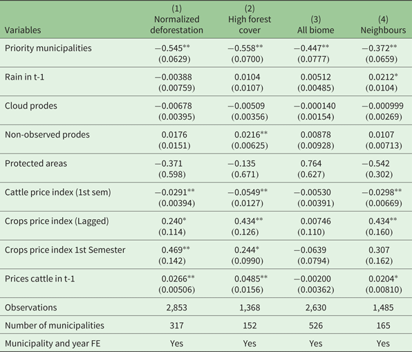
Table 1 shows the effect of the MPs policy on Amazon deforestation. All specifications include municipality and time fixed effects along with controls for rain, image quality (clouds Prodes and Non-observed Prodes), price, and existence of protected areas.
The effect of blacklisting on deforestation in the Amazon Biome

Notes: Significance: **p<0.01, *p<0.05. Normalized deforestation is the dependent variable in all specifications. Column 1 presents coefficients for our main specification, as described in section 4. Column 2 uses a restricted sample of municipalities with more than half of their territory covered by native vegetation in the first sample year. Column 3 restricts the sample to the years after 2006, and uses the whole Amazon Biome in the sample to allow for comparison with the regressions we later run using the number of fines and DETER cloud coverage. Column 4 presents the results of the regression using the neighbours as a control group.
Column 1 presents coefficients for our main specification, as described in section 4. Column 2 uses a restricted sample of municipalities with more than half of their territory covered by native vegetation in the first sample year. Column 3 uses the share of municipality area deforested instead of normalized deforestation as the dependent variable. Column 4 restricts the sample to the years after 2006, and uses the whole Amazon Biome in the sample to allow for comparison with the regressions we later run using the number of fines and DETER cloud coverage (as data on DETER cloud coverage is only available starting in 2006 and cloud coverage is a strong instrument for fines only when using all municipalities of the Amazon Biome).
Priority municipalities appear to have a negative and significant impact on deforestation. Results are robust to all specifications. Quantitatively, counterfactual analysis shows that the policy avoided the clearing of 11,396 km2 of Amazon forest area in our sample from 2008 through 2011. Total deforestation observed in the sample in the same period was 20,689 km2, 35.1 per cent smaller than in the absence of the policy.
5.2 Robustness exercises
5.2.1 Deforestation pre-trends
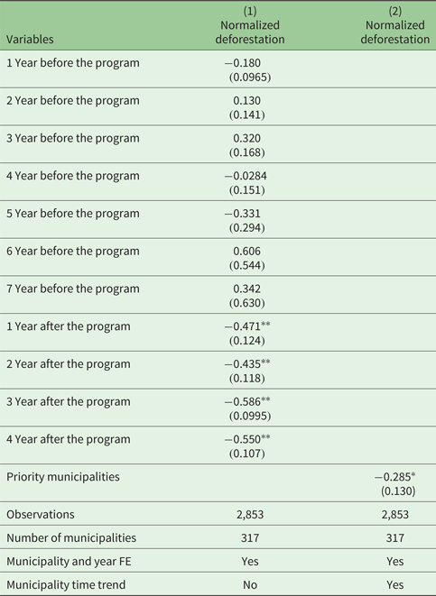
To make sure that our results have not been driven by different deforestation trends between treatment and control groups, we present some robustness exercises to show that deforestation pre-trends were similar among both groups. Table 2 suggests that our results are not coming from differences in deforestation pre-policy trends. In column 1 we build dummies showing since when the municipality was in the priority list and dummies showing how much time that year is before the municipality becomes a priority municipality. In this case, the dummy ‘1 Year after the program’ means that the municipality becomes priority in that same year, the dummy ‘2 Years after the program’ means the municipality becomes priority in the previous year, and so on. The same logic was used to build the dummies ‘X Years before the program’. We see that only the dummies indicating post-policy priority status have a significant effect on deforestation. The pre-treatment dummies are not statistically significant, indicating that different pre-policy deforestation trends are likely not a concern for our specifications. Even so, in column 2, we run our benchmark specification (the same as for column 1, table 1), but now controlling for municipality-specific time trends (e.g., a municipality dummy interacted with a linear time trend). The MPs policy still appears to have a significant negative effect on deforestation. Thus, it seems that we are really capturing the policy effect on deforestation, and not that of pre-policy trends.
Pre-trend regressions

Notes: Significance: **p < 0.01, *p < 0.05. In column 1 we build dummies showing since when the municipality was in the priority list and dummies showing how much time that year is before the municipality becomes a priority municipality. In this case, the dummy ‘1 Year after the program’ means that the municipality becomes priority in that same year, the dummy ‘2 Years after the program’ means the municipality becomes priority in the previous year, and so on. The same logic was used to build the dummies ‘X Years before the program’. In column 2, we run our benchmark specification (the same as column 1, table 1), but now controlling for municipality-specific time trends (e.g., a municipality dummy interacted with a linear time trend).
5.2.2 Pre-trends and spillovers in other characteristics
The pre-trend test on deforestation provides confidence about parallel trends. However, how some other variables affect deforestation in the Amazon matters and could be driving our results. For example, it is possible that municipalities with more protected areas have a different trend in deforestation from municipalities without protected areas. In this case, even after controlling for fixed effects, not only does the variation of protected areas matters, but also the relationship of protected areas ‘level’ and deforestation trends.
Another worry related to protected areas is the interaction effects via spillover. Protected areas could not only affect deforestation in the same municipality but could also build a barrier to expansion of agriculture and deforestation, which could affect deforestation in the neighbourhood (Herrera, Reference Herrera2015).
To deal with these facts, we do two different exercises. First, we control to an interaction between the average share of the municipality territory covered by Protected Areas before 2008 and a linear time trend. This exercise allows municipalities with different coverage in protected areas to have different deforestation trends. Second, we control for the protected areas in neighbour municipalities (where neighbours here are defined as bordering municipalities).
The deforestation literature also provides evidence about other factors that drive deforestation in the Amazon, such as roads, vegetation type, agricultural growing, etc. Although we control for fixed effects, it is possible that the levels of some of these variables affects deforestation even after controlling for fixed effects through affecting trends (Pfaff et al., Reference Pfaff, Robalino, Walker, Aldrich, Caldas, Reis, Perz, Bohrer, Arima and Laurance2007, Reference Pfaff, Robalino, Lima, Sandoval and Herrera2014, Reference Pfaff, Robalino, Herrera and Sandoval2015).
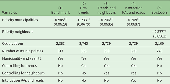
Therefore, we also include in these exercises other variables besides protected areas. In table 3, column 1, we repeat our benchmark specification (that of column 1, table 1). In column 2, we include controls for interaction between variables before 2008 and a linear time trend. In this exercise, besides protected areas, we include number of head of cattle per km2 (annual average before 2008), share of the territory with soybean plantation (annual average before 2008), credit per km2 (annual average before 2008), per capita GDP (annual average before 2008), roads (we only have data from 2010, so this is what we use), and poverty (we only have data from 2000, so this is what we use). All these variables are interacted with a linear time trend and added as controls for the main specification. We also included in this regression, for the variables for which we have time-series variation (number of head of cattle per km2, share of the territory with soybean plantation, credit per km2 and per capita GDP), the variables themselves as a control. Results presented in column 2 show that the impact of MPs did not change much.
Controlling for trends, and spillovers

Notes: Significance: **p < 0.01. In column 1, we repeat our benchmark specification. In column 2, we include controls for interaction between variables before 2008 and a linear time trend. In this exercise, besides protected areas, are included number of head of cattle per km2 (annual average before 2008), share of the territory with soybean plantation (annual average before 2008), credit per km2 (annual average before 2008), per capita GDP (annual average before 2008), roads (from 2010), and poverty (from 2000). All these variables are interacted with a linear time trend and added as controls. We also included in this regression, for the variables for which we have time-series variation (number of head of cattle per km2, share of the territory with soybean plantation, credit per km2, and per capita GDP) the variables themselves as a control. In column 3, we add controls for neighbours' information on: share of protected areas, number of head of cattle per km2, share of the territory with soybean plantation, credit per km2, and per capita GDP. We also control for interactions between a linear time trend and roads, and poverty in the neighbours. In column 4, we interact the linear trend in roads with protected areas and add it as a control. In column 5, we consider municipalities that are neighbouring priority municipalities as our treatment group. As a control group, we use the municipalities that border the priority municipalities' neighbours, but are not priority municipalities themselves.
At the same way, some of these variables have spatial interactions. Therefore, for the variables for which we have time-varying observations, we control for these variables in neighbours' municipalities, in the same way as for the protected areas case. Then, we control for neighbours' information on: share of protected areas, number of head of cattle per km2, share of the territory with soybean plantation, credit per km2 and per capita GDP. We also control for interactions between a linear time trend and roads, and poverty in the neighbours and for the same set of controls already included in column 2. Results are presented in column 3 of table 3 and again did not change the impact of MPs on deforestation.
In column 4 of table 3, besides all the controls used in column 3, we also interact the linear trend in roads with protected areas. More specifically, for each municipality, we first build interaction terms between a linear time trend and the density of roads in 2010. We then interact these specific trends with the share of the municipal area covered by PAs. The idea here is that the interaction between protected areas and roads could be an even stronger determinant of deforestation trends. In order to avoid the possibility that our results are being driven by the correlation between this strong determinant of deforestation trends and MPs, we include the control mentioned above. Results show that the MPs dummy remains negative and significant to explain deforestation after the inclusion of all these controls.
5.2.3 Priority municipalities' spillovers and leakage
Finally, we run an extra exercise to try to identify leakage. To do so, we now consider the municipalities that are neighbours to MPs (in the sense that they border the MPs) as our treatment group. As a control group, we use the municipalities that border the MPs' neighbours but are not MPs themselves. The assumption is that if there is leakage (negative spillovers), farmers increase deforestation in municipalities as close as possible to the priority ones. This could be a problem for our estimation because it means that the net effect of the policy could be zero. If there are positive spillovers, farmers reduce deforestation also in municipalities close to the priority ones, which means that our estimation is a lower bound of the effect of MPs on deforestation.
The idea to rationalize positive spillovers is that producers become afraid to be caught when they see monitoring increasing for the neighbours. If, in this exercise, the effect on this new treatment group is zero, it means that there is no leakage and there is no positive spillover. The results are presented in table 3, column 5, and show that deforestation decreases also for the neighbours of the MPs compared to the neighbours of the neighbours. This in turn means that there are positive spillover effects of MPs to their neighbours and our main results are a lower bound of the effects of MPs on deforestation. These results are in line with the ones found in Andrade (Reference Andrade2016).
5.2.4 Alternative normalized measures
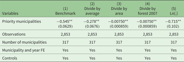
Thus far our results have proven robust to different robustness exercises. However, to confirm the robustness of the effect of MPs on deforestation in the Amazon, we test different normalization measures to our dependent variable, deforestation rate. Table 4 presents the results of the regressions of our benchmark specification on different dependent variables. In column 1, we repeat our benchmark normalization measure, the same one as in table 1, column 1. In column 2, we regress the same equation but now using total deforestation divided by deforestation average of each municipality as the dependent variable. Column 3 does the same thing but dividing by municipality area. In column 4, we divide our deforestation measure by the stock of forest of each municipality one year before the creation of the priority list (that is, the year 2007). The idea here is that not only is the municipality size important, but also how much the municipality still had to deforest. Finally, in column 5, we use the natural logarithm of deforestation as our dependent variable. In all these specifications, the MPs dummy remains negatively significant to explain deforestation, which means that our results do not depend on the normalization choice.
Alternative normalized measures

Notes: Significance: **p < 0.01. Column 1 repeats our benchmark results, with our original normalized measure. column 2 uses total deforestation divided by deforestation average of each municipality as dependent variable. Column 3 does the same thing but dividing by municipality area. In column 4, we divide our deforestation measure by the forest cover of each municipality in 2007, one year before the creation of the priority list. Finally, in column 5, we use natural logarithm of deforestation as our dependent variable.
5.3 Direct impact of blacklisting on production, credit and fines
Finally, we investigate the mechanism through which the policy was most effective. To do this, we calculate the impact of the policy on the number of fines applied by Ibama and on other economic variables (credit concessions and agricultural production). These variables are used with the same normalization as the deforestation variable.
The trade-off between conservation and income growth is a well-studied topic in the environmental economics literature. A good starting point for understanding the theoretical framework discussed by the authors is whether there is an environmental Kuznets curve (EKC). Grossman and Krueger (Reference Grossman and Krueger1995) find that, for some pollutants, economic growth initially deteriorates the environment, and then improves the environment at income levels above US$8,000 per capita. The theoretical and empirical literature on the EKC develops this relationship between income and the environment, both from the point of view of the country's income growth and of the income growth of individuals. The idea is that poorer individuals will pay more attention to problems related to the satisfaction of emergency needs than to environmental amenities, while richer individuals will have a marginally greater utility in consuming these amenities. With the inclusion of environmental variables in the utility function of consumers, markets would move toward less polluting technological production structures (Selden and Song, Reference Selden and Song1994; Plassmann and Khanna, Reference Plassmann and Khanna2006; Ranjan and Shortle, Reference Ranjan and Shortle2007).
From the point of view of political economy, better institutions are better able to establish conservation policies for the environment and punishment criteria that avoid incentives for environmental degradation. Therefore, as there is a positive correlation between income and institutions (Acemoglu et al., Reference Acemoglu, Johnson and Robinson2001), as incomes increase, institutions become stronger and improve their capacity to create laws and mechanisms to control environmental quality (Kaika and Zervas, Reference Kaika and Zervas2013).
There is much criticism of this literature on the EKC. While there is some consensus about an inverted U-relationship between income and SO2 and NO2 emissions, the same does not seem to be true for CO2 emissions, which continue to grow even after countries become very wealthy, which would increase concerns with regard to the problems of climate change and global warming (Stern et al., Reference Stern, Common and Barbier1996; Stern and Common, Reference Stern and Common2001; Yandle et al., Reference Yandle, Vijayaraghavan and Bhattarai2002).
Moreover, methodological problems have been pointed out in this literature, especially because of the difficulty in establishing a causal relationship between the variables in question, per capita income and environmental amenities (Stern et al., Reference Stern, Common and Barbier1996; Stern and Common, Reference Stern and Common2001).
There is also a more specific literature dealing with the theme of income growth and forest preservation. Cropper and Griffiths (Reference Cropper and Griffiths1994) find evidence of an EKC for forests in Latin America and Africa, that is, income growth increases deforestation for very low incomes but decreases deforestation for very high incomes. Antle and Heidebrink (Reference Antle and Heidebrink1995) find a positive relationship between reforestation and income when income is above a certain cut-off point and Foster and Rosenzweig (Reference Foster and Rosenzweig2003) provide evidence that there is no relationship between income and plant cover in open economies, but there is a positive relationship between the two variables in closed economies. The subject, therefore, is controversial in the literature; there is no consensus. In this paper we contribute to this literature by measuring the impact of a specific conservation policy in the Brazilian Amazon on agricultural production.
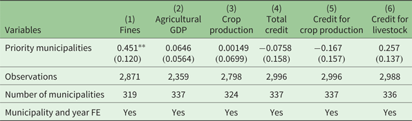
Table 5 shows the impact of the policy on the number of fines, credit concessions and agricultural production. Results indicate that the policy had effect only on the number of fines, with no effect on credit concessions and agricultural production. It seems that the mechanism through which the policy had effect on deforestation was the increase in monitoring intensity and quality, since it had no effects on economic variables.
The effect of blacklisting on fines, agricultural production and credit concessions

Notes: Significance: **p < 0.01, The table presents the impact of priority municipalities on the number of fines (column 1), agricultural GDP (column 2), crop production value (column 3), total rural credit lent (column 4), rural credit lent for crop production (column 5), and rural credit lent for livestock activities (column 6).
Results do not support a trade-off between conservation and agricultural production. They suggest that it would be possible to contain forest clearings without significantly compromising local agricultural production. Although informative, this exercise is not entirely conclusive. The effect may have resulted from agricultural producers responding to stricter law enforcement by shifting from a low-productivity set-up to a more productive one. In this sense, production that was lost at the extensive margin may have been compensated for by production at the intensive one. Moreover, not having an immediate adverse effect on average agricultural production does not mean that MPs had no effect at all. If farmers adjust production over time, our sample period might not be sufficient to capture this effect. If individual data was available yearly, we could also measure heterogeneity in the effect of conservation policy on agricultural production. For example, policy could constrain small-scale farmers' production, but this could be offset by large scale producers farming more intensively. Future investigations of this topic, once data become available, could shed light on the matter.
5.4 The monitoring and law enforcement channel
We also run similar regressions as in table 1, but controlling for the number of fines applied by Ibama, as instrumented by DETER cloud coverage. Table A1 in the online appendix shows the results. The results show that, when adequately controlling for law enforcement, the MPs policy has no significant impact on deforestation.
Taken together, these results suggest that the impact of the MPs policy stems from increased monitoring and improved law enforcement in these municipalities. Other potential consequences of being classified as a PM, such as economic sanctions, appear to have had no significant effect on Amazon deforestation. Of course, part of the effect on better monitoring these municipalities would be attributed to increasing political pressure, but the lack of effect on economic variables withdraws the possibility of economic forces driving the deforestation reduction in MPs.
6. Conclusion
We show that the blacklist created by the Brazilian government in 2008 was an effective tool to combat deforestation. In principle, this policy could work by improving the instruments of monitoring and law enforcement or serving as the basis for additional political and economic pressures, as suggested in some studies. Our results suggest that the monitoring and law enforcement channel prevails over the other efforts.
The paper yields two main policy implications. First, maintaining targeted monitoring and law enforcement activities in the Brazilian Amazon is important in order to continue reducing deforestation. The MPs has successfully targeted law enforcement activities, thereby reducing deforestation in municipalities which were responsible for an important part of deforestation in the Amazon Biome before the policy implementation. Second, our findings show that the policy change had no effect on agricultural production. This finding reinforces the case for relying on monitoring and law enforcement to reduce deforestation.
Finding ways of reducing deforestation in the Amazon is important for at least two reasons. On the one hand, the Amazon has the largest stock of rainforests and biodiversity in the world. Given the institutional and governance limitations in place, finding effective ways of controlling deforestation in such an environment has global consequences. On the other hand, the concept of a well-targeted monitoring system based on satellite imagery can be applicable to other contexts, especially in developing countries where law enforcement is challenging.
Supplementary Material
The supplementary material for this article can be found at https://doi.org/10.1017/S1355770X18000499.
Acknowledgements
Assuncão acknowledges financial support from the CNPq (Brazilian National Council for Scientific and Technological Development).