1 Introduction
Processes such as turbulence, diffusion and particle acceleration are ubiquitous both in astrophysical and laboratory plasmas. Understanding particle diffusion is of fundamental importance in order to characterize the distribution of the charged gas in the universe and, more specifically, in the heliosphere. The understanding of the energetic particles motion, originating for example from solar flares or coronal mass ejections, can help preventing injuries for space travellers, as well as hardware damage to satellites. Moreover the distribution of heavy ions in the Earth’s magnetosphere can have effects on climate changes (Luo et al. Reference Luo, Kronberg, Nykyri, Trattner, Daly, Chen, Du and Ge2017). Particle transport theory is fundamental for the dynamics of the solar corona (Lepreti et al. Reference Lepreti, Carbone, Abramenko, Yurchyshyn, Goode, Capparelli and Vecchio2012) and of the interplanetary medium (Ruffolo, Matthaeus & Chuychai Reference Ruffolo, Matthaeus and Chuychai2003, Reference Ruffolo, Matthaeus and Chuychai2004). In laboratory plasma experiments, the magnetic confinement could be improved by understanding what affects particle turbulent transport (Taylor & McNamara Reference Taylor and McNamara1971; Hauff et al. Reference Hauff, Pueschel, Dannert and Jenko2009).
Charged particle dynamics depends on the stochastic motion of the magnetic field lines. The random walk of the magnetic field lines affects the diffusion both across and along the mean magnetic field (Jokipii & Parker Reference Jokipii and Parker1969). Particles gyrate along the magnetic field but, if the field is turbulent, they spread in the perpendicular direction (Chandran et al. Reference Chandran, Li, Rogers, Quataert and Germaschewski2010; Ruffolo et al. Reference Ruffolo, Pianpanit, Matthaeus and Chuychai2012), ‘jumping’ from one field line to another. The turbulent nature of space and laboratory plasmas suggests that the best way to describe their dynamics is given by the statistical approach (Green Reference Green1951; Jokipii Reference Jokipii1966). In this statistical (Lagrangian) description, particles move in a turbulent electromagnetic field, similarly to the motion of neutral tracers in atmospheric turbulence (Richardson Reference Richardson1926; Kolmogorov Reference Kolmogorov1941). The turbulent nature of the fields that scatter the particles makes the analytical treatment rather difficult. Because of this, we still lack an exact and universal theory to describe diffusion (Bieber & Matthaeus Reference Bieber and Matthaeus1997; Hussein & Shalchi Reference Hussein and Shalchi2016).
A common theoretical approach, applied when studying diffusion of charged particles, relies on calculating separately the diffusion coefficient in the directions parallel and perpendicular to the main guiding field (Jokipii Reference Jokipii1966; Subedi et al. Reference Subedi, Sonsrettee, Blasi, Ruffolo, Matthaeus, Montgomery, Chuychai, Dmitruk, Wan and Parashar2017). Currently the nonlinear guiding centre (NLGC) theory (Matthaeus et al. Reference Matthaeus, Qin, Bieber and Zank2003) gives a rather accurate prediction of the diffusion coefficient for systems with a three-dimensional (3-D) geometry. However, a full 3-D description of plasma turbulence requires huge computational efforts that can be streamlined by reducing the dimensionality of the problem. In fact, if a strong guiding magnetic field is present, turbulence becomes anisotropic and a simpler 2-D model may become a good approximation. In this scenario, the structures and phenomena related to turbulence, such as current sheets and reconnecting magnetic islands (Matthaeus & Lamkin Reference Matthaeus and Lamkin1986; Greco et al. Reference Greco, Matthaeus, Servidio, Chuychai and Dmitruk2009a ; Servidio et al. Reference Servidio, Greco, Matthaeus, Osman and Dmitruk2011b ), magnetic field topology changes and energy conversion (Parker Reference Parker1957; Matthaeus, Ambrosiano & Goldstein Reference Matthaeus, Ambrosiano and Goldstein1984; Ambrosiano et al. Reference Ambrosiano, Matthaeus, Goldstein and Plante1988; Servidio et al. Reference Servidio, Matthaeus, Shay, Cassak and Dmitruk2009, Reference Servidio, Valentini, Perrone, Greco, Califano, Matthaeus and Veltri2015), mainly occur due to dynamics in the plane perpendicular to the main field (Bruno & Carbone Reference Bruno and Carbone2016). Currently, magnetic reconnection is considered one of the most effective mechanisms for particle acceleration and energization (Zank et al. Reference Zank, le Roux, Webb, Dosch and Khabarova2014), being crucial for explosive events in the solar atmosphere, like solar flares (Cargill et al. Reference Cargill, Vlahos, Turkmani, Galsgaard and Isliker2006, Reference Cargill, Vlahos, Baumann, Drake and Nordlund2012; Cadavid et al. Reference Cadavid, Lawrence, Christian, Jess and Nigro2014) and coronal mass ejections (Gosling Reference Gosling2010). Analogously, in the Earth’s magnetosphere (Drake et al. Reference Drake, Swisdak, Che and Shay2006; Oka et al. Reference Oka, Phan, Krucker, Fujimoto and Shinohara2010; Birn et al. Reference Birn, Artemyev, Baker, Echim, Hoshino and Zelenyi2012) and in the distant outer heliosphere (Lazarian & Opher Reference Lazarian and Opher2009), magnetic reconnection is thought to be a very active mechanism.
We aim to study the diffusion problem and to test the existing theories by using self-consistent simulations of plasma turbulence, where the back reaction of particle dynamics over the fields is taken into account. Together with diffusion, we study the acceleration and energization of particles (Lazarian & Opher Reference Lazarian and Opher2009; Tessein et al. Reference Tessein, Matthaeus, Wan, Osman, Ruffolo and Giacalone2013; Zank et al. Reference Zank, le Roux, Webb, Dosch and Khabarova2014; le Roux et al. Reference le Roux, Zank, Webb and Khabarova2015), especially in regions where magnetic reconnection is expected to occur.
The present work is organized as follows. In § 2 we will present a global overview on the model that describes the plasmas in the low-collisionality limit. We will introduce the numerical algorithm that simulates the plasma particle dynamics. In § 3, the particle trajectory statistics will be presented, interpreting the numerical results via the plasma turbulent diffusion theories. The investigation of the acceleration process will be the central topic of § 4, where we will perform local analysis of the acceleration phenomenon. Finally, in the last section, we will present the discussions, conclusions and future perspectives.
2 Simulations of 2.5-D plasma turbulence
We perform three hybrid-PIC (particle in cell) simulations, varying the ion plasma
 $\unicode[STIX]{x1D6FD}$
, defined as the ratio between the thermal and the magnetic pressures, namely
 $\unicode[STIX]{x1D6FD}=P_{\text{cin}}/P_{B}=v_{\text{th}}^{2}/v_{\text{A}}^{2}$
, with
 $v_{\text{th}}$
and
 $v_{\text{A}}$
being the initial thermal and the Alfvén speed (related to the mean field
 $B_{0}$
), respectively. This parameter has been set equal for ions and electrons, namely
 $\unicode[STIX]{x1D6FD}_{i}=\unicode[STIX]{x1D6FD}_{e}\equiv \unicode[STIX]{x1D6FD}$
. We performed runs with
 $\unicode[STIX]{x1D6FD}=5$
, 0.5 and 0.1, in order to cover a wide range of relevant plasma scenarios. These chosen values are such that the high
 $\unicode[STIX]{x1D6FD}$
value is typical of plasmas found in the Earth’s magnetosheath; the value of
 $\unicode[STIX]{x1D6FD}=0.5$
is close to the typical solar wind conditions, whereas the lowest
 $\unicode[STIX]{x1D6FD}$
is appropriate for solar corona and laboratory devices.
2.1 Model equations
Particles and fields are described by the Vlasov–Maxwell system (2.1) that we solve via a hybrid-PIC approach, using kinetic ions and fluid electrons. The system of normalized equations is given by
 $$\begin{eqnarray}\displaystyle \left.\begin{array}{@{}c@{}}\dot{\boldsymbol{x}}=\boldsymbol{v},\\ \dot{\boldsymbol{v}}=\boldsymbol{E}+\boldsymbol{v}\times \boldsymbol{B},\\ \displaystyle {\displaystyle \frac{\unicode[STIX]{x2202}\boldsymbol{B}}{\unicode[STIX]{x2202}t}}=-\unicode[STIX]{x1D735}\times \boldsymbol{E},\\ \displaystyle \boldsymbol{E}=-(\boldsymbol{u}\times \boldsymbol{B})+{\displaystyle \frac{1}{n}}\,\boldsymbol{j}\times \boldsymbol{B}-\frac{1}{n}\unicode[STIX]{x1D735}P_{e}+\unicode[STIX]{x1D702}\boldsymbol{j}.\end{array}\right\} & & \displaystyle\end{eqnarray}$$
In the above equations,
 $\boldsymbol{x}$
is the particle position,
 $\boldsymbol{v}$
the velocity,
 $\boldsymbol{E}$
is the electric field,
 $\boldsymbol{B}$
is the magnetic field,
 $n=\int f\,\text{d}\boldsymbol{v}$
is the proton number density,
 $\boldsymbol{u}=(1/n)\int \boldsymbol{v}f\,\text{d}\boldsymbol{v}$
is the proton bulk velocity and
 $\boldsymbol{j}=\unicode[STIX]{x1D735}\times \boldsymbol{B}$
is the current density. In the above definitions
 $f(\boldsymbol{x},\boldsymbol{v},t)$
is the velocity distribution function of the ions. The pressure term is adiabatic
 $P_{e}=\unicode[STIX]{x1D6FD}n^{\unicode[STIX]{x1D6FE}}$
and
 $\unicode[STIX]{x1D702}=0.006$
is the resistivity that introduces a small-scale dissipation, for numerical stability. The electric field is given by the generalized Ohm’s law. In the simulations distances are normalized to the proton inertial length
 $d_{p}=c/\unicode[STIX]{x1D714}_{p_{i}}$
, where
 $c$
is the speed of light and
 $\unicode[STIX]{x1D714}_{p_{i}}$
is ion plasma frequency. The time is normalized to
 $\unicode[STIX]{x1D6FA}_{cp}^{-1}$
, that is the ion cyclotron frequency. Finally, velocities are normalized to the Alfvén speed
 $v_{\text{A}}=c\unicode[STIX]{x1D6FA}_{cp}/\unicode[STIX]{x1D714}_{p_{i}}$
.
The three simulations have the same initial conditions: uniform density and a Maxwellian distribution of the particles’ velocities with uniform temperature. We impose large-scale fluctuations in order to mimic the motion of the large energy-containing vortices. We have chosen random fluctuations, at large scale, for both magnetic field and the ion bulk velocity field. The (2.1) are solved on a square grid of size
 $L_{0}=128d_{p}$
, discretized with
 $512^{2}$
points, with periodic boundary conditions. This initial state consists of a 2-D spectrum of fluctuations, perpendicular to the main field
 $B_{0}$
(the latter chosen along
 $z$
). The fluctuations amplitude is
 $\unicode[STIX]{x1D6FF}b/B_{0}\sim 0.3$
. To suppress the statistical noise of the PIC method we use 1500 particles per cell (approximately
 $4\times 10^{8}$
total particles).
2.2 Characteristics of plasma turbulence
Turbulence properties are fundamental for the modelling and the understanding of the transport of charged particles. In this subsection we will highlight the statistical properties of kinetic turbulence, together with important analyses such as the power spectra of the fluctuations and the characteristic length scales of turbulence. The latter two analyses will be crucial for the theoretical modelling of turbulent diffusion and particle acceleration.
To describe the magnetic topology, in the 2.5-D approximation, it is useful to define the in-plane magnetic field as
 $\boldsymbol{B}_{\bot }=\unicode[STIX]{x1D735}a_{z}\times \hat{\boldsymbol{z}}$
, where
 $a_{z}$
is the magnetic potential and
 $\hat{z}$
is the out-of-plane (axial) unit vector. The current in the axial direction is
 $j_{z}=(\unicode[STIX]{x1D735}\times \boldsymbol{B}_{\bot })\boldsymbol{\cdot }\hat{z}=-\unicode[STIX]{x1D6FB}^{2}a_{z}$
. To achieve a stationary state of fully developed turbulence, we initially let the system to freely decay, and then we introduce a forcing at the time
 $t^{\ast }$
at which nonlinearity reaches its peak (roughly the peak of
 $\langle j_{z}^{2}\rangle$
), namely
 $t^{\ast }\sim 25\unicode[STIX]{x1D6FA}_{cp}^{-1}$
. The forcing consists of ‘freezing’ the amplitude of the large-scale modes of the in-plane magnetic field, with
 $1\leqslant m\leqslant 4$
, leaving the phases unchanged. This corresponds to a large-scale input of energy, as described in Servidio et al. (Reference Servidio, Haynes, Matthaeus, Burgess, Carbone and Veltri2016).
In order to have meaningful statistics, we perform our analysis when a steady state has been achieved, namely for
 $50<t\unicode[STIX]{x1D6FA}_{cp}<250$
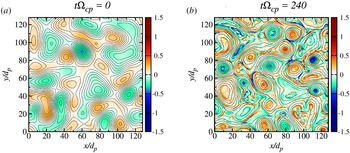
. Figure 1 shows the shaded contour of the current density
 $j_{z}$
along with the contour line of the vector potential
 $a_{z}$
, as the system evolves toward turbulence. Panel (a) shows the initial state of the system, where islands and current sheets are not defined yet. As time goes on, smaller vortices and sharp current sheets develop. In particular, these magnetic structures represent magnetic islands (flux tubes in three dimensions). The global appearance of the system remains unchanged, in a statistical sense, when the peak of nonlinearity has been reached. Regions of intense magnetic gradient appear in between reconnecting magnetic islands, with associated intense current sheets (Matthaeus & Montgomery Reference Matthaeus and Montgomery1980; Servidio et al.
Reference Servidio, Valentini, Perrone, Greco, Califano, Matthaeus and Veltri2015).
Current density
 $j_{z}$
(colour map) together with vector potential
 $a_{z}$
(contour lines), at the initial state (a), with big structures and tenuous axial current, and at the final state (b), with coherent structures such as small vortices and intense current sheets. The most intense current sheets are located in between reconnecting magnetic islands (Matthaeus & Montgomery Reference Matthaeus and Montgomery1980).

To better describe the state of fully developed turbulence, we computed the Fourier spectra, as a function of the wavenumber
 $|\boldsymbol{k}|$
, of both the electric and the magnetic fields. The power spectra for the trace of the correlation tensor,
 $|\tilde{\boldsymbol{B}}(\boldsymbol{k},t)|^{2}$
, where
 $\tilde{\boldsymbol{B}}(\boldsymbol{k},t)$
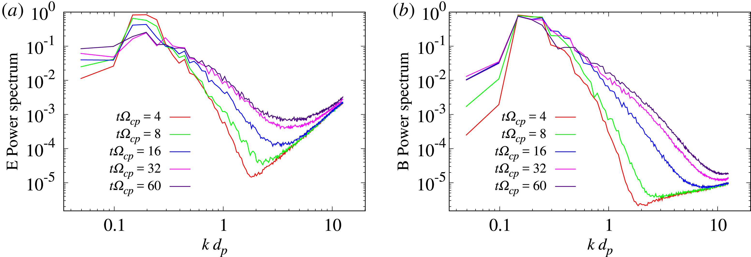
are the respective Fourier coefficients, are reported in figure 2. These spectra exhibit the classical scenario of magnetohydrodynamics (MHD) turbulence, in which energy flows from large to small scales. This cascade of energy occurs over the so-called inertial subrange, where energy scales as
 $k^{-5/3}$
(Bruno & Carbone Reference Bruno and Carbone2016). In particular, figure 2 shows the turbulent development. The state of fully developed turbulence is achieved after
 $50\unicode[STIX]{x1D6FA}_{cp}^{-1}$
. After this time the spectra are almost stationary (do not experience large fluctuations). It is important to note, that as observed in the solar wind (Bale et al.
Reference Bale, Kellogg, Mozer, Horbury and Reme2005), the power in the electric fields is higher, at
 $k$
values that correspond to characteristic ion lengths. This is in agreement with previous studies and simulations of plasma turbulence (Howes et al.
Reference Howes, Dorland, Cowley, Hammett, Quataert, Schekochihin and Tatsuno2008; Matthaeus, Servidio & Dmitruk Reference Matthaeus, Servidio and Dmitruk2008; Franci et al.
Reference Franci, Landi, Matteini, Verdini and Hellinger2015).
Power spectra of the electric (a) and the magnetic (b) fields as a function of the wavenumber (normalized with the proton inertial length
 $d_{p}$
), at different times. While turbulence develops, energy is transferred from the large to the small scales. In the steady state, at
 $k\sim d_{p}^{-1}$
, the electric field spectrum manifests a steeper slope.

In order to understand the dynamics of particles in a turbulent scenario, where structures are present at different scales, it is useful to measure different characteristic lengths. The correlation (or integral) length of a turbulent field generally corresponds approximately to the size of the largest energy-containing turbulent eddies, (in our case the typical sizes of the islands). This length can be obtained from the two-point correlation function
 $C(\boldsymbol{r})$
as
 $$\begin{eqnarray}\displaystyle \unicode[STIX]{x1D706}_{C}=\int _{\unicode[STIX]{x1D6FA}}C(\boldsymbol{r})\,\text{d}\boldsymbol{r}={\displaystyle \frac{1}{\langle b^{2}\rangle }}\int _{\unicode[STIX]{x1D6FA}}\text{d}\boldsymbol{r}\langle \boldsymbol{b}(\boldsymbol{x}+\boldsymbol{r})\boldsymbol{\cdot }\boldsymbol{b}(\boldsymbol{x})\rangle . & & \displaystyle\end{eqnarray}$$
Here
 $\boldsymbol{b}$
represents the magnetic fluctuations and
 $\langle \cdot \rangle$
is the average over the total volume
 $\unicode[STIX]{x1D6FA}$
. Note that fluctuations are isotropic in the plane perpendicular to the main field, hence
 $\boldsymbol{x}$
and
 $\boldsymbol{r}$
are in-plane vectors and the above length is essentially the same, namely
 $C(r_{x})\sim C(r_{y})\equiv C(\boldsymbol{r})$
. Moreover,
 $\unicode[STIX]{x1D706}_{C}$
is very similar for the bulk velocity fluctuations, because of the choice of the initial conditions and the driving. In the above definitions we suppressed the time dependence because of stationarity, and we computed these lengths averaging over time, in the steady state regime. For our system
 $\unicode[STIX]{x1D706}_{C}\sim 10d_{p}$
and does not vary for runs with different plasma
 $\unicode[STIX]{x1D6FD}$
.
Apart from the above energy-containing scale, which is a large scale characteristic length of turbulence, it is important to characterize also the properties at smaller scales. In hydrodynamics the Taylor length is the scale at which the viscous dissipation term is no longer negligible (Servidio et al. Reference Servidio, Greco, Matthaeus, Osman and Dmitruk2011b ). This scale is related to the largest width of the structures, where dissipation starts to be relevant. In our case, the magnetic Taylor scale can be defined as
 $$\begin{eqnarray}\displaystyle \unicode[STIX]{x1D706}_{T}=\sqrt{{\displaystyle \frac{b_{\bot }^{2}}{\langle j_{z}^{2}\rangle }}}. & & \displaystyle\end{eqnarray}$$
In the above expression,
 $b_{\bot }$
is the root mean square of the magnetic field in the plane perpendicular to the axial direction (perpendicular to the main guiding field), and
 $\langle j_{z}^{2}\rangle$
is the axial current density averaged over the perpendicular plane, and averaged also over the times in which the system is in the stationary state of fully developed turbulence. This scale can be considered as the scale at which the inertial range of turbulence terminates (Frisch Reference Frisch1995). In our simulations
 $\unicode[STIX]{x1D706}_{T}\sim 1.7d_{p}$
. Since the Taylor length
 $\unicode[STIX]{x1D706}_{T}$
gives the largest size of the dissipative structures, we introduce now an average measure of these structures, namely the typical width of the layer cores (X-points). The current sheet width,
 $\unicode[STIX]{x1D6FF}_{c}$
, is the half-maximum width of the current sheet intensity profile. The average core width of the current sheets we measured as
 $\unicode[STIX]{x1D6FF}_{c}\sim 0.3d_{p}$
.
3 Particle diffusion in plasma turbulence
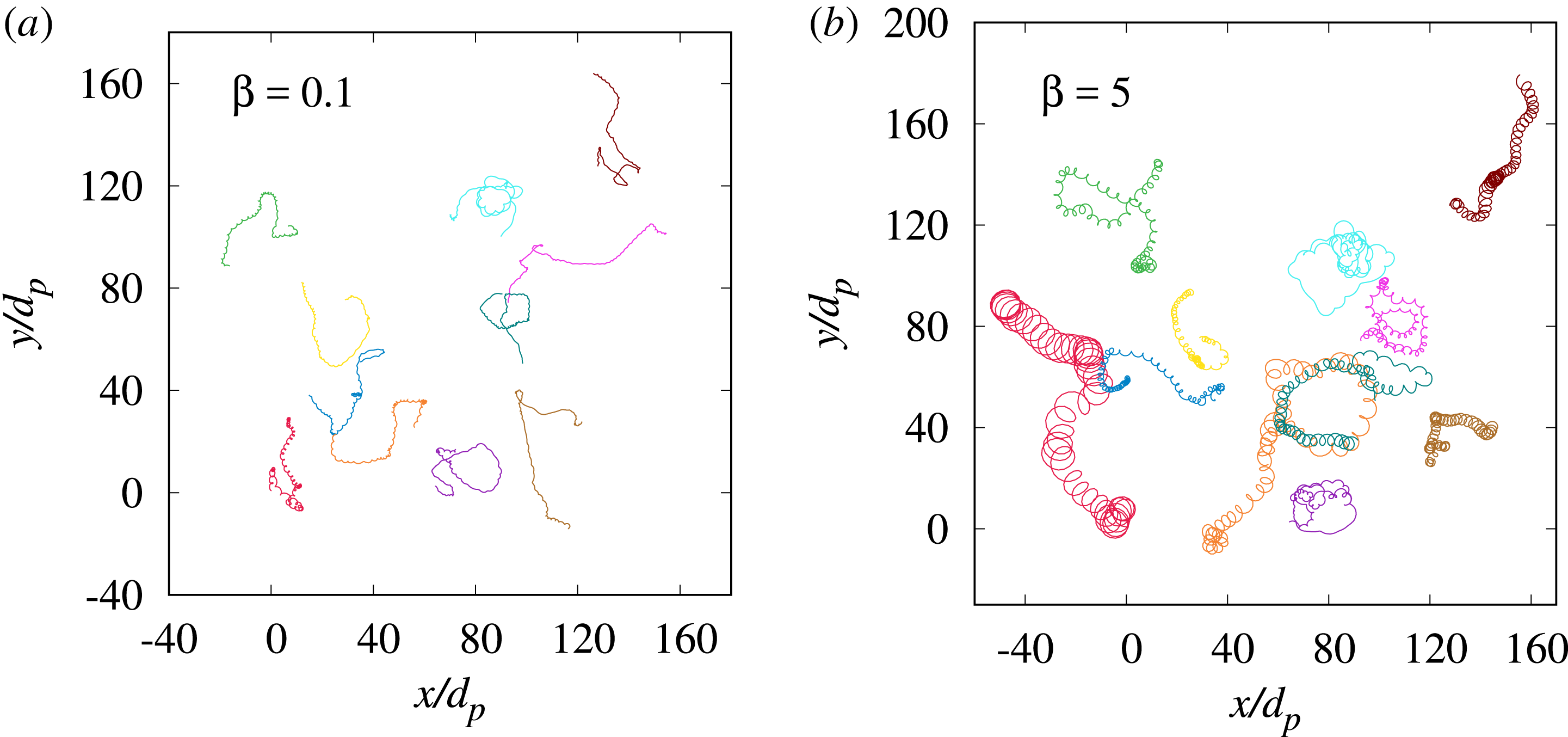
Particle trajectories for
 $\unicode[STIX]{x1D6FD}=0.1$
(a) and
 $\unicode[STIX]{x1D6FD}=5$
(b). It is possible to observe that particles in the high
 $\unicode[STIX]{x1D6FD}$
plasma have bigger Larmor radii, while particles in the low
 $\unicode[STIX]{x1D6FD}$
one move almost in straight lines, with more abrupt changes of direction. One can notice that some particles have closed orbits as they are trapped in a magnetic island while others experience sudden bendings of their trajectory.

We now investigate the particle motion in steady state turbulence. We have followed the path of
 $10^{5}$
among all the PIC macro-particles, verifying the convergence of the statistical results. From their positions as a function of time, it is possible to compute the diffusion coefficient, measuring their mean squared displacement. After a general overview on the erratic trajectory of particles in 2.5-D turbulence, we will see whether the plasma
 $\unicode[STIX]{x1D6FD}$
affects the statistics of ion diffusion and acceleration.
In figure 3 we show the 2-D projections of the trajectories of some randomly selected particles, during the whole simulation, for two distinct values of
 $\unicode[STIX]{x1D6FD}$
(low and high
 $\unicode[STIX]{x1D6FD}$
). As can be seen, particles that move in the high
 $\unicode[STIX]{x1D6FD}$
plasma are less magnetized and their Larmor radii are large. Particles in the low-
 $\unicode[STIX]{x1D6FD}$
plasma, instead, are highly magnetized and perform tight gyrations, with more abrupt changes of direction. Small-
 $\unicode[STIX]{x1D6FD}$
particles spread less than in the high
 $\unicode[STIX]{x1D6FD}$
case. Generally, in all cases, one can notice that some particles have closed orbits as they are trapped in a magnetic island while others experience turnovers that suddenly bend the trajectory. As we shall see, particles that perform closed trajectories are mostly trapped in turbulent vortices, whereas sharply segmented trajectories can belong to particles which encounter local intense turbulent structures, such as magnetic discontinuities or current sheets, that make them deviate suddenly (Drake et al.
Reference Drake, Opher, Swisdak and Chamoun2010; Haynes, Burgess & Camporeale Reference Haynes, Burgess and Camporeale2014).
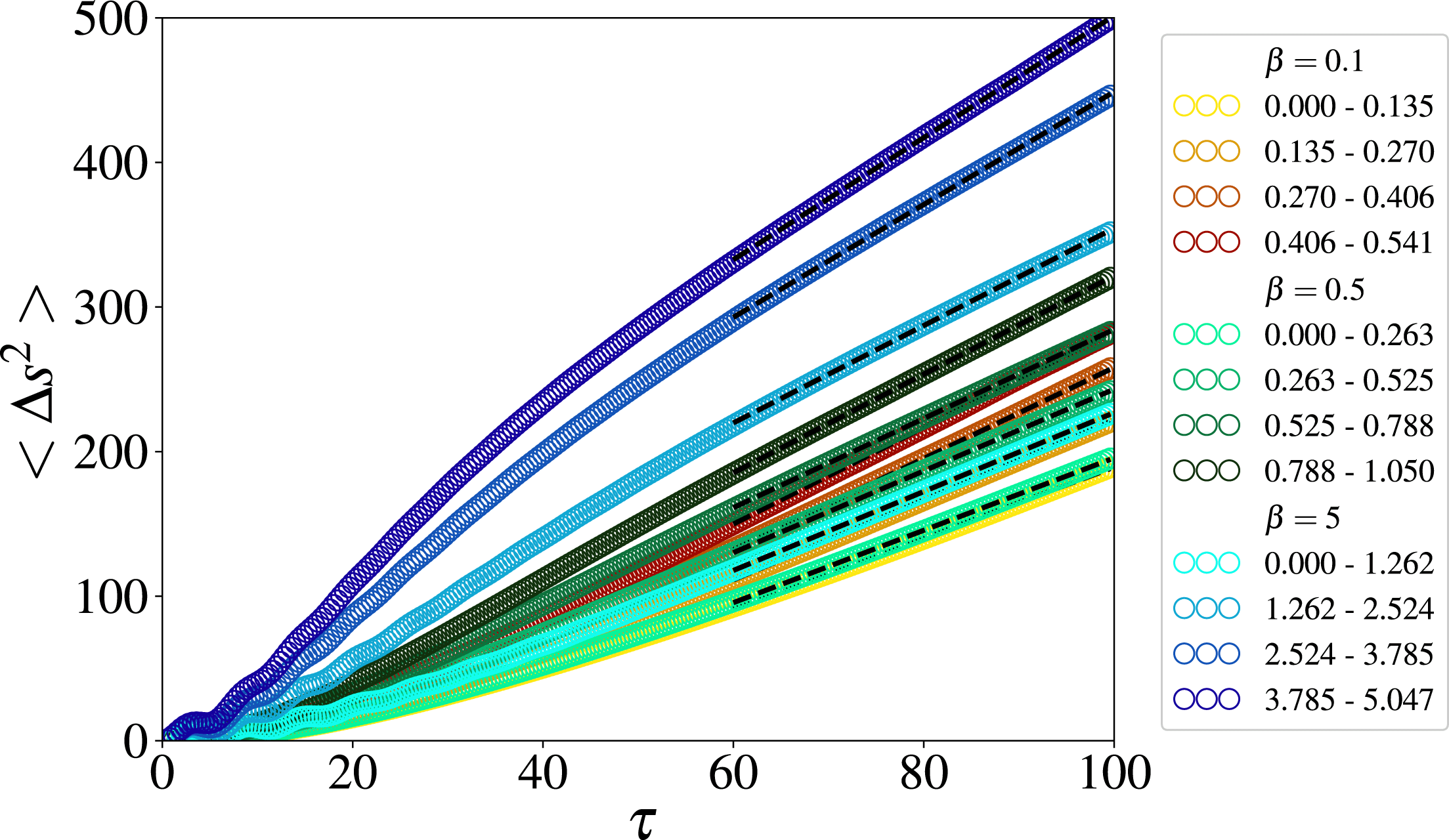
Mean squared displacement in the perpendicular plane as a function of the time interval
 $\unicode[STIX]{x1D70F}$
(cyclotron units), for several particle energy ranges, indicated in the label, for the three different
 $\unicode[STIX]{x1D6FD}$
values. For short times, it is possible to observe a deviation from the linear prediction of the Brownian motion (3.1). The normal diffusion is achieved for rather large time intervals, namely
 $\unicode[STIX]{x1D70F}>60\unicode[STIX]{x1D6FA}_{cp}^{-1}$
, where we extrapolate the values of the diffusion coefficient
 $D$
via linear fits (dashed lines).

The overall motion, as represented in figure 3, seems quite random: particles scatter and diffuse in time. We computed the square displacement
 $\unicode[STIX]{x0394}s^{2}=\unicode[STIX]{x0394}x^{2}+\unicode[STIX]{x0394}y^{2}$
with
 $\unicode[STIX]{x0394}x=x(t)-x(t_{0})$
and
 $\unicode[STIX]{x0394}y=y(t)-y(t_{0})$
. We define the time lag
 $\unicode[STIX]{x1D70F}=t-t_{0}$
, relative to a varying origin
 $t_{0}$
, a procedure justified by stationarity in this steady state regime. We found that, for sufficiently long time intervals, the motion is diffusive (Chandrasekhar Reference Chandrasekhar1943), namely
 $$\begin{eqnarray}\displaystyle \langle \unicode[STIX]{x0394}s^{2}\rangle =2D\unicode[STIX]{x1D70F}. & & \displaystyle\end{eqnarray}$$
In the above expression,
 $D$
is the diffusion coefficient,
 $\unicode[STIX]{x1D70F}$
is the time interval over which the particle moves by
 $\unicode[STIX]{x0394}s$
and the brackets now represent an ensemble average computed over particles. To understand the dependence of the diffusion coefficient on particle parallel energy, namely
 $v_{z}^{2}$
(the kinetic energy associated with the component parallel to the mean magnetic field), we divide the particles into energy bins, whose values are normalized with respect to the squared Alfvén speed
 $(c_{_{\text{A}}}^{2})$
, and evaluate the above diffusion coefficient. The averaged mean squared displacement as a function of the time interval for several energy values is shown in figure 4. It is possible to observe that the normal diffusive behaviour is achieved for
 $\unicode[STIX]{x1D70F}\gtrsim 60\unicode[STIX]{x1D6FA}_{cp}^{-1}$
. By fitting the curves after this threshold value with (3.1), we can obtain the numerical value of
 $D$
. For shorter time intervals particles seem not to follow the linear law. Indeed, for short time intervals the particle motion cannot be stochastic since they have a ‘memory’ of their initial condition, and a temporal correlations exists. It is clear that the higher the particle energy, the larger the diffusion coefficient. Before reporting the numerical results on the diffusion of particles in self-consistent kinetic simulations, we will introduce the theoretical background.
3.1 A nonlinear guiding centre (NLGC) model in two dimensions
Currently, a useful description of perpendicular diffusion is given by the nonlinear guiding centre (NLGC) theory (Matthaeus et al.
Reference Matthaeus, Qin, Bieber and Zank2003). This theory works well for 3-D turbulence, with a uniform mean magnetic field, and it has been validated with test-particle simulations and observations (Bieber et al.
Reference Bieber, Matthaeus, Shalchi and Qin2004; Shalchi, Bieber & Matthaeus Reference Shalchi, Bieber and Matthaeus2004). We want to develop a theory that can describe particle diffusion in the 2.5-D approximation turbulence, and test it with the self-consistent plasma simulations. In the following, we will describe the main steps of the 3-D NLGC derivation, considering the particle gyromotion. Using the Taylor–Green–Kubo (TGK) formulation (Taylor Reference Taylor1922; Green Reference Green1951; Kubo Reference Kubo1957; Shalchi & Dosch Reference Shalchi and Dosch2008; Shalchi Reference Shalchi2015), one can write the diffusion coefficient
 $D_{xx}$
, for instance along the
 $x$
direction, as
 $$\begin{eqnarray}\displaystyle D_{xx}={\displaystyle \frac{1}{B_{0}^{2}}}\int _{0}^{\infty }\text{d}\unicode[STIX]{x1D70F}\langle v_{z}(0)B_{x}(\boldsymbol{x}(0),0)v_{z}(\unicode[STIX]{x1D70F})B_{x}(\boldsymbol{x}(\unicode[STIX]{x1D70F}),\unicode[STIX]{x1D70F})\rangle , & & \displaystyle\end{eqnarray}$$
where it is assumed that the particle motion projected onto the 2-D plane follows the 2-D projection of the magnetic field lines. We assume that the magnetic field fluctuations in the perpendicular plane are completely uncorrelated with the velocity in the
 $z$
direction and this allows us to write the diffusion coefficient as
 $$\begin{eqnarray}\displaystyle D_{xx}={\displaystyle \frac{1}{B_{0}^{2}}}\int _{0}^{\infty }\text{d}\unicode[STIX]{x1D70F}\langle v_{z}(0)v_{z}(\unicode[STIX]{x1D70F})\rangle \langle B_{x}(\boldsymbol{x}(0),0)B_{x}(\boldsymbol{x}(\unicode[STIX]{x1D70F}),\unicode[STIX]{x1D70F})\rangle . & & \displaystyle\end{eqnarray}$$
To develop the 2.5-D version of the theory, we modify 3-D NLGC by saying that the velocity correlation function in the
 $z$
direction is nothing but the square value of the
 $z$
velocity i.e.
 $$\begin{eqnarray}\displaystyle \langle v_{z}(0)v_{z}(\unicode[STIX]{x1D70F})\rangle \sim v_{z}^{2}. & & \displaystyle\end{eqnarray}$$
This assumption has been directly validated by measuring the quantity
 $\langle v_{z}(0)v_{z}(\unicode[STIX]{x1D70F})\rangle$
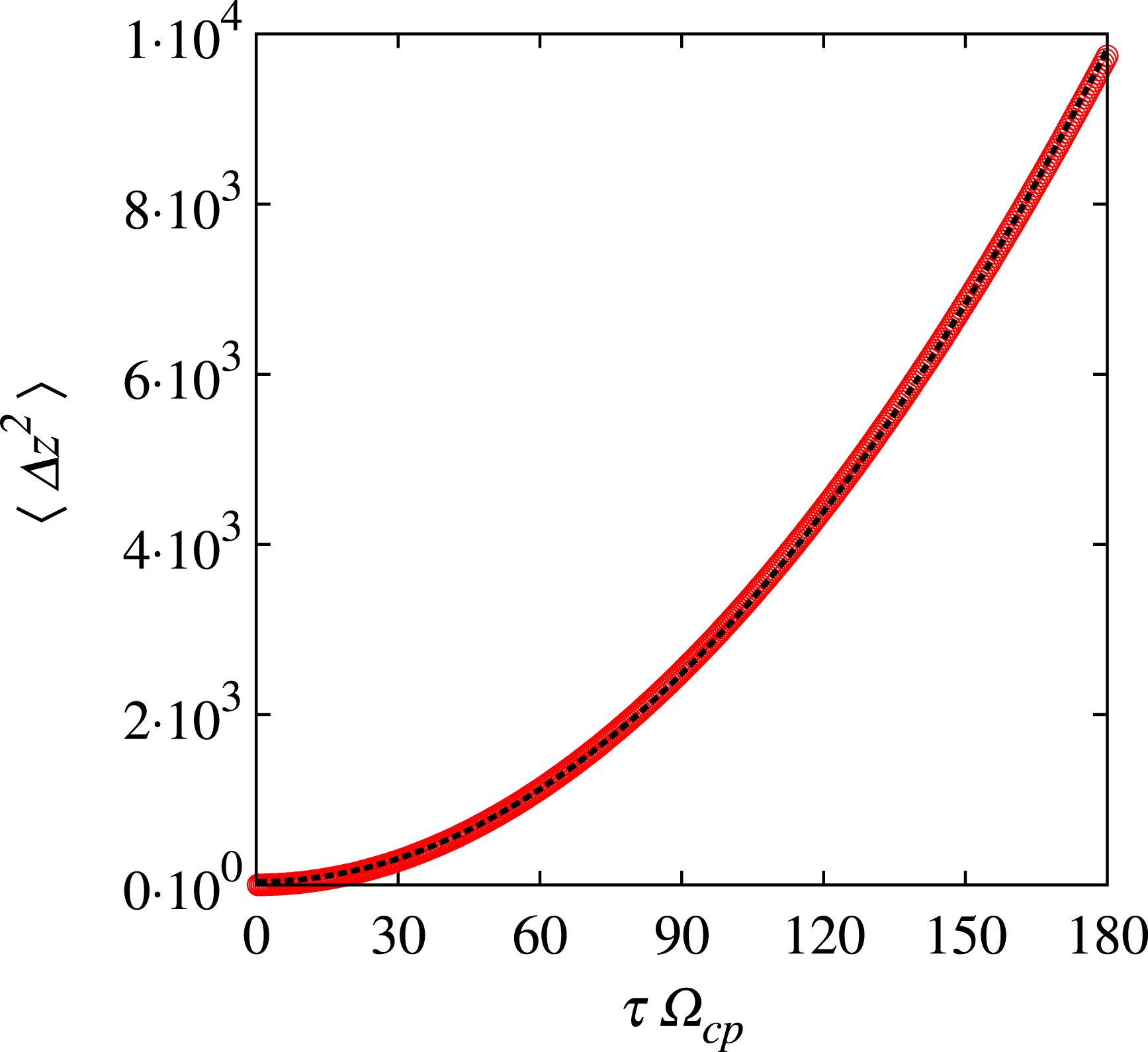
in our simulations. Figure 5 shows that the motion along
 $z$
is given by free streaming, with
 $\langle \unicode[STIX]{x0394}z^{2}\rangle \sim t^{2}$
and therefore the velocity
 $v_{z}$
, in the direction along the main field, is almost constant.
Mean squared displacement in the
 $z$
direction averaged over all the particles as a function of
 $\unicode[STIX]{x1D70F}$
. The dashed line is the parabolic fit (
 $\propto \unicode[STIX]{x1D70F}^{2}$
). For every
 $\unicode[STIX]{x1D6FD}$
, the assumption of free streaming made in (3.4) is relatively solid.

Using this approximation, we can estimate the diffusion coefficient neglecting the parallel scattering, and get:
 $$\begin{eqnarray}\displaystyle D_{xx}={\displaystyle \frac{v_{z}^{2}}{B_{0}^{2}}}\int _{0}^{\infty }\text{d}\unicode[STIX]{x1D70F}\langle B_{x}(\boldsymbol{x}(0),0)B_{x}(\boldsymbol{x}(\unicode[STIX]{x1D70F}),\unicode[STIX]{x1D70F})\rangle . & & \displaystyle\end{eqnarray}$$
Using Corrsin’s independence hypothesis to transform the integrand function as
 $$\begin{eqnarray}\displaystyle \langle B_{x}(\boldsymbol{x}(0),0)B_{x}(\boldsymbol{x}(\unicode[STIX]{x1D70F}),\unicode[STIX]{x1D70F})\rangle =\int \text{d}\boldsymbol{r}\unicode[STIX]{x1D619}_{xx}(\boldsymbol{r},\unicode[STIX]{x1D70F})P(\boldsymbol{r},\unicode[STIX]{x1D70F}) & & \displaystyle\end{eqnarray}$$
one arrives at
 $$\begin{eqnarray}\displaystyle D_{xx}={\displaystyle \frac{v_{z}^{2}}{B_{0}^{2}}}\int _{0}^{\infty }\text{d}\unicode[STIX]{x1D70F}\int \text{d}\boldsymbol{r}\unicode[STIX]{x1D619}_{xx}(\boldsymbol{r},\unicode[STIX]{x1D70F})P(\boldsymbol{r},\unicode[STIX]{x1D70F}), & & \displaystyle\end{eqnarray}$$
where
 $\unicode[STIX]{x1D619}_{xx}(\boldsymbol{r},\unicode[STIX]{x1D70F})$
is the Eulerian two-point two-time correlation tensor and
 $P(\boldsymbol{r},\unicode[STIX]{x1D70F})$
is the probability function of a particle having displacement
 $\boldsymbol{r}$
after a time interval
 $\unicode[STIX]{x1D70F}$
(Matthaeus et al.
Reference Matthaeus, Qin, Bieber and Zank2003). At this point, it is convenient to express
 $\unicode[STIX]{x1D619}_{xx}(\boldsymbol{r},\unicode[STIX]{x1D70F})$
using its Fourier transform
 $$\begin{eqnarray}\displaystyle \unicode[STIX]{x1D619}_{xx}(\boldsymbol{r},\unicode[STIX]{x1D70F})=\int \text{d}\boldsymbol{k}S_{xx}(\boldsymbol{k},\unicode[STIX]{x1D70F})\text{e}^{\text{i}\boldsymbol{k}\boldsymbol{\cdot }\boldsymbol{r}}. & & \displaystyle\end{eqnarray}$$
We can model
 $S_{xx}(\boldsymbol{k},\unicode[STIX]{x1D70F})=S_{xx}(\boldsymbol{k})\unicode[STIX]{x1D6E4}(\boldsymbol{k},\unicode[STIX]{x1D70F})$
, where
 $\unicode[STIX]{x1D6E4}(\boldsymbol{k},\unicode[STIX]{x1D70F})$
represents the time propagator of the spectrum, and
 $S_{xx}(\boldsymbol{k})$
is the spatial spectrum. Usually, this functional form is described via the so-called sweeping decorrelation mechanism, namely
 $\unicode[STIX]{x1D6E4}(\boldsymbol{k},\unicode[STIX]{x1D70F})\sim \text{e}^{-\unicode[STIX]{x1D70F}/\unicode[STIX]{x1D70F}_{c}(\boldsymbol{k})}$
, where
 $\unicode[STIX]{x1D70F}_{c}(\boldsymbol{k})$
is a characteristic decorrelation time. The latter is usually thought to be the ‘sweeping decorrelation time’ (Chen & Kraichnan Reference Chen and Kraichnan1989; Nelkin & Tabor Reference Nelkin and Tabor1990), in analogy with fluid turbulence (see below).
At this point, we can proceed with the theoretical estimate of the diffusion coefficient, given by
 $$\begin{eqnarray}\displaystyle D_{xx}={\displaystyle \frac{v_{z}^{2}}{B_{0}^{2}}}\int _{0}^{\infty }\int \text{d}\boldsymbol{k}S_{xx}(\boldsymbol{k})\,\text{d}\unicode[STIX]{x1D70F}\unicode[STIX]{x1D6E4}(\boldsymbol{k},\unicode[STIX]{x1D70F})\int \text{d}\boldsymbol{r}P(\boldsymbol{r},\unicode[STIX]{x1D70F})\text{e}^{\text{i}\boldsymbol{k}\boldsymbol{\cdot }\boldsymbol{r}}. & & \displaystyle\end{eqnarray}$$
Since
 $P$
is Gaussian, then
 $$\begin{eqnarray}\displaystyle \int \text{d}\boldsymbol{r}P(\boldsymbol{r},\unicode[STIX]{x1D70F})\text{e}^{\text{i}\boldsymbol{k}\boldsymbol{\cdot }\boldsymbol{r}}=\text{e}^{-(k_{x}^{2}D_{xx}+k_{y}^{2}D_{yy})\unicode[STIX]{x1D70F}}. & & \displaystyle\end{eqnarray}$$
In axisymmetric turbulence
 $D_{xx}=D_{yy}\equiv D$
,
 $S_{xx}=S_{yy}\equiv S$
and, since we have only in-plane structures (i.e.
 $k_{z}=0$
)
 $k_{x}^{2}+k_{y}^{2}\equiv k^{2}$
, the diffusion coefficient is
 $$\begin{eqnarray}\displaystyle D={\displaystyle \frac{v_{z}^{2}}{B_{0}^{2}}}\int \text{d}\boldsymbol{k}S(\boldsymbol{k})\int _{0}^{\infty }\text{d}\unicode[STIX]{x1D70F}\text{e}^{-k^{2}D\unicode[STIX]{x1D70F}}\text{e}^{-\unicode[STIX]{x1D70F}/\unicode[STIX]{x1D70F}_{c}(\boldsymbol{k})}. & & \displaystyle\end{eqnarray}$$
Finally, integrating over
 $\unicode[STIX]{x1D70F}$
, one gets
 $$\begin{eqnarray}\displaystyle D={\displaystyle \frac{v_{z}^{2}}{B_{0}^{2}}}\int \text{d}\boldsymbol{k}{\displaystyle \frac{S(\boldsymbol{k})}{[\unicode[STIX]{x1D70F}_{C}(k)]^{-1}+k^{2}D}}. & & \displaystyle\end{eqnarray}$$
Note that this prediction is only a small modification to the 3-D NLGC theory, having suppressed the
 $z$
-dependence by using the particle free streaming along
 $z$
(3.4).
In order to obtain a first estimate of the diffusion coefficient
 $D$
, we can make an approximation. Assuming that the sweeping decorrelation time is rather long (as in the case of large-scale slow driving, for example), we can drop the term
 $\unicode[STIX]{x1D70F}_{C}(k)^{-1}$
in (3.12). This latter term, indeed, makes the equation more complex to solve. We therefore obtain:
 $$\begin{eqnarray}\displaystyle D^{\ast }\sim \sqrt{{\displaystyle \frac{v_{z}^{2}}{B_{0}^{2}}}\int \text{d}\boldsymbol{k}{\displaystyle \frac{S(\boldsymbol{k})}{k^{2}}}}. & & \displaystyle\end{eqnarray}$$
The reader may notice that this result is essentially of the same form of the so-called field line random walk (FLRW) limit of perpendicular particle scattering (Jokipii Reference Jokipii1966; Bieber & Matthaeus Reference Bieber and Matthaeus1997). For such cases,
 $D=v_{eff}D_{fl}$
where
 $D_{fl}$
is the Fokker–Planck coefficient for field line transport, and
 $v_{eff}$
is the effective velocity of the particle along the magnetic field (Matthaeus et al.
Reference Matthaeus, Gray, Pontius and Bieber1995).
To evaluate the diffusion coefficient via (3.12) and (3.13) we computed the average power spectrum
 $S(\boldsymbol{k})$
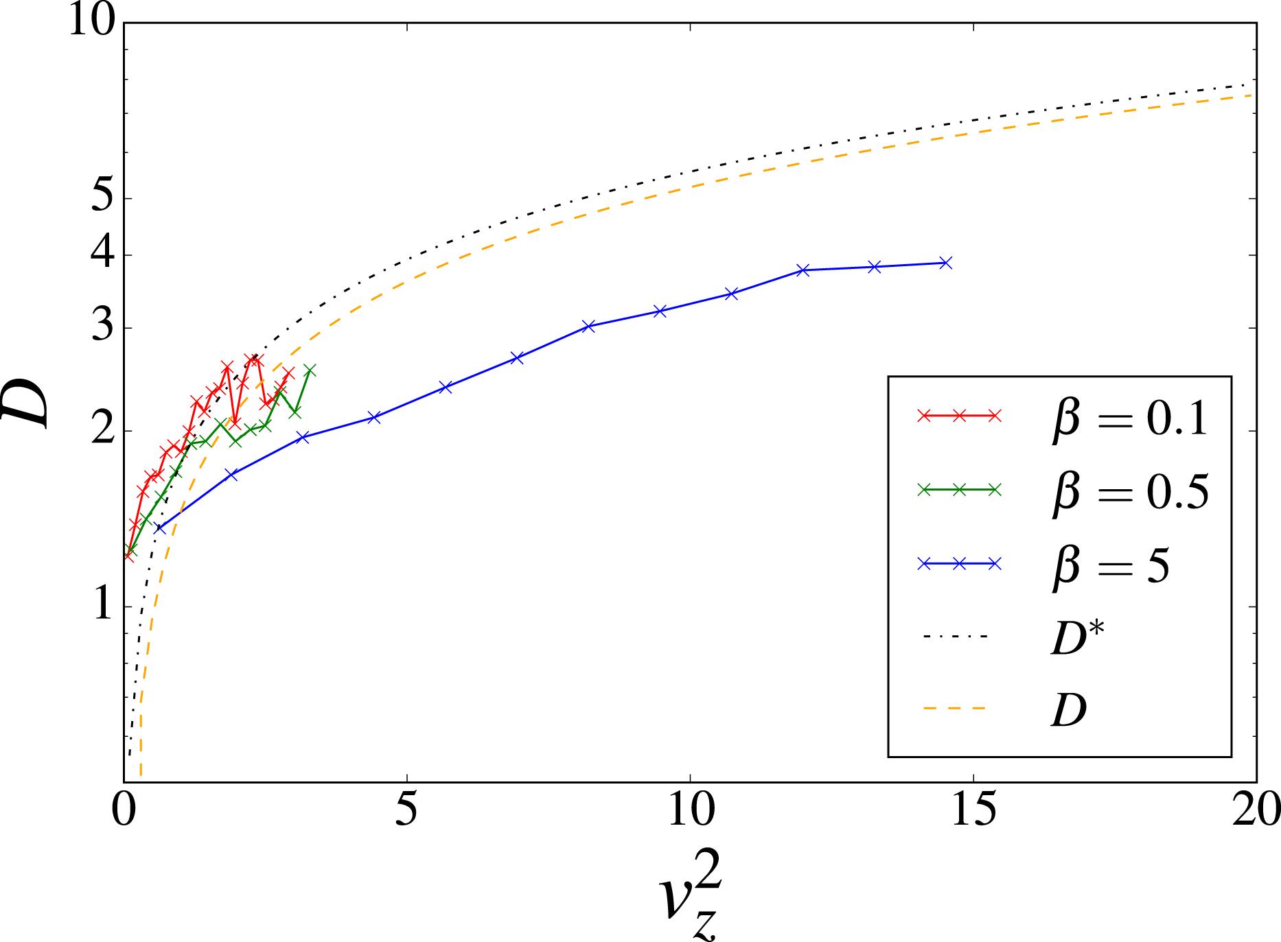
from the simulations. Figure 6 shows the numerical values of
 $D$
obtained by fitting the particles mean squared displacements in figure 4. The theoretical values of the 2-D NLGC, evaluated via both the exact and the approximated formulas, are reported as a function of the particles energies. The simulation results follow fairly well the theoretical prediction at low
 $\unicode[STIX]{x1D6FD}$
. The theory slightly deviates at very high energy (
 $\unicode[STIX]{x1D6FD}$
values), although the functional monotonic behaviour is very similar.
The diffusion coefficient as a function of the parallel energy
 $v_{z}^{2}$
, calculated by fitting the mean square displacement (red, green and blue line–points, respectively for
 $\unicode[STIX]{x1D6FD}=0.1$
, 0.5 and 5) for all the simulations. The theoretical diffusion coefficient from the approximated 2-D NLGC theory (3.13) is reported with the black point–dashed line whereas the exact calculation (3.12) is the orange dashed line.

Here we briefly investigate the decorrelation mechanism in self-consistent, plasma turbulence. We performed a Fourier transform in time of the magnetic fluctuations, computing the propagator
 $\unicode[STIX]{x1D6E4}(k,\unicode[STIX]{x1D70F})$
, as described in Servidio et al. (Reference Servidio, Carbone, Dmitruk and Matthaeus2011a
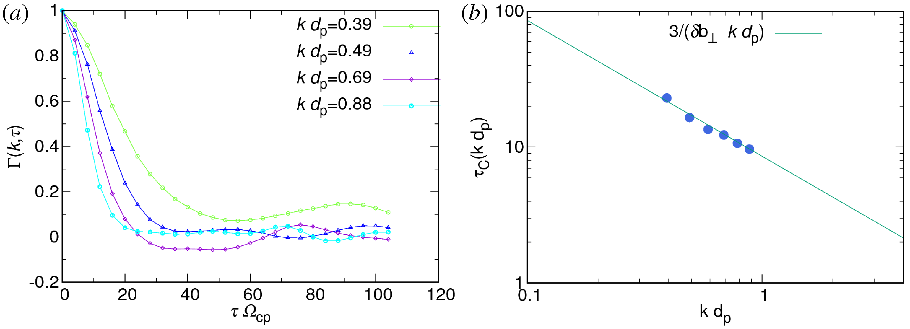
), Perri et al. (Reference Perri, Servidio, Vaivads and Valentini2017). As in fluid, MHD, and Hall MHD models of turbulence, this time-dependent correlation of turbulence strongly depends on the amplitude of
 $k$
, as reported in figure 7. As it can be seen, the decorrelation mechanism depends on
 $k$
and drops quickly in time (only a few inertial range modes are reported). From this functional form, we computed the decorrelation time
 $\unicode[STIX]{x1D70F}_{C}(k)$
, represented in (b) of the same figure. The decorrelation time scales as
 ${\sim}1/k$
, indicating the clear dominance of the sweeping effect. To be more quantitative, in order to compute the diffusion coefficient for our experiment, we found that
 $\unicode[STIX]{x1D70F}_{C}(k)\sim 3/(\unicode[STIX]{x1D6FF}b_{\bot }kd_{p})$
, where
 $\unicode[STIX]{x1D6FF}b_{\bot }$
is the root mean square (r.m.s.) of the in-plane magnetic fluctuations.
(a) Propagator of the magnetic field spectrum, computed for several (perpendicular)
 $k$
modes in the inertial range of plasma turbulence. (b) Decorrelation time as a function of
 $k$
(blue bullets), computed as the
 $e$
-folding time of the functional form in (a). The sweeping prediction is reported with the solid teal line.

4 Particle acceleration
In agreement with previous literature (Jokipii & Parker Reference Jokipii and Parker1969; Matthaeus et al. Reference Matthaeus, Qin, Bieber and Zank2003), we have found that diffusivity depends on particle energy. The behaviour of diffusion is in agreement with a modified model of the NLGC theory, here adapted to collisionless 2.5-D plasmas. Moreover, we observed that many of these particles experience variations of their momentum – namely an acceleration process. In this section, we investigate the mechanisms responsible for acceleration, using conditional statistics. We will establish the relationship between the effectiveness of the acceleration mechanism and the particles’ energies, and the existence of possible resonance conditions that energize the ions.
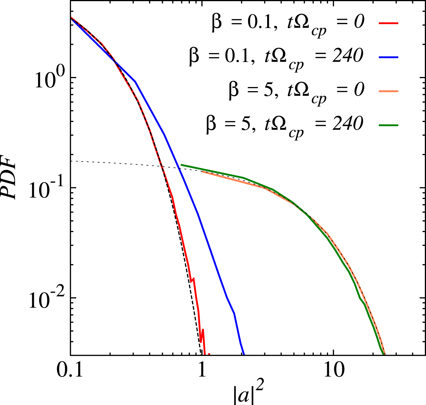
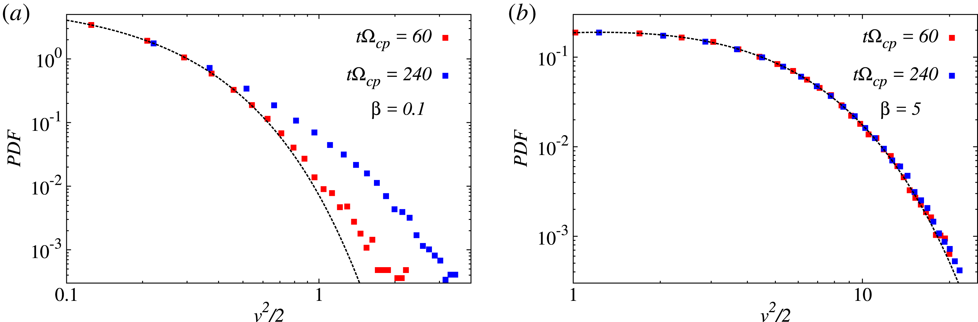
PDFs of the particles’ acceleration, for
 $\unicode[STIX]{x1D6FD}=0.1$
and
 $\unicode[STIX]{x1D6FD}=5$
. Both the initial and the final times of the simulations are reported, together with the corresponding probability distributions for a random variable (dashed black lines). In the low
 $\unicode[STIX]{x1D6FD}$
case, extreme acceleration processes are observed.

We have computed, for each particle, the Lagrangian acceleration
 $\boldsymbol{a}=\unicode[STIX]{x2202}\boldsymbol{v}/\unicode[STIX]{x2202}t$
, where
 $\boldsymbol{v}$
is the particle velocity. We computed the probability density function (PDF) of the Lagrangian acceleration, for all the particles, at different times and for different simulations. The acceleration has been computed by using a sixth-order finite difference (centred) method. The distributions are reported in figure 8, for the two extreme
 $\unicode[STIX]{x1D6FD}$
’s, at the beginning and at the end of the simulation. As can be observed, the PDFs of the particles’ acceleration in the high
 $\unicode[STIX]{x1D6FD}$
plasma are well described by the
 $\unicode[STIX]{x1D712}^{2}$
distribution that is defined as
 $$\begin{eqnarray}\displaystyle \text{PDF}(\unicode[STIX]{x1D712}_{k}^{2})={\displaystyle \frac{1}{2^{k}\unicode[STIX]{x1D6E4}(k/2)}}x^{k/2-1}\text{e}^{-x/2}, & & \displaystyle\end{eqnarray}$$
where
 $k$
, commonly referred to as the ‘degrees of freedom’, represents the number of a set of independent normally distributed variables
 $\{x_{1},x_{2},\ldots ,x_{k}\}$
, and
 $\unicode[STIX]{x1D6E4}(x)$
is the gamma function. The sum of the square of these
 $k$
variables is distributed according to the
 $\unicode[STIX]{x1D712}_{k}^{2}$
PDF. In our case the three independent variables are the acceleration components
 $\{a_{x},a_{y},a_{z}\}$
and the square modulus of the acceleration
 $|a|^{2}=a_{x}^{2}+a_{y}^{2}+a_{z}^{2}$
, distributed according to the
 $\unicode[STIX]{x1D712}_{3}^{2}$
with 3 degrees of freedom.
For
 $\unicode[STIX]{x1D6FD}=5$
, in particular, this distribution does not change in time, indicating the lack of very extreme events during the evolution of the system. Whereas at low
 $\unicode[STIX]{x1D6FD}$
(
 $\unicode[STIX]{x1D6FD}=0.1$
), the acceleration, which is initially randomly distributed, develops a tail at later times (blue solid line). This means that the number of particles with an anomalous acceleration is higher for low
 $\unicode[STIX]{x1D6FD}$
plasma, suggesting that a physical process that depends on the plasma conditions is at work.
A straightforward acceleration mechanism can be due to an electric field parallel to the local magnetic field:
 $$\begin{eqnarray}\displaystyle E_{\Vert }={\displaystyle \frac{\boldsymbol{E}\boldsymbol{\cdot }\boldsymbol{B}}{|\boldsymbol{B}|}}. & & \displaystyle\end{eqnarray}$$
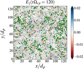
We identified the anomalous particles, i.e. the particles with acceleration values exceeding the variance of the followed distribution and represented their positions, at a given time, over the parallel electric field map with a contour plot of the magnetic potential in the
 $z$
direction, in order to see whether they show a correlation with the turbulent structures. This map is reported in figure 9. The figure shows that particles with anomalous acceleration are affected by the above field: these ions are non-uniformly distributed, they cluster where the parallel electric field is more intense, on the flanks of the magnetic islands.
Particles with very high acceleration (green dots), superimposed on the shaded contour of the parallel electric field. These particles are localized in the regions where the parallel electric field is bigger.

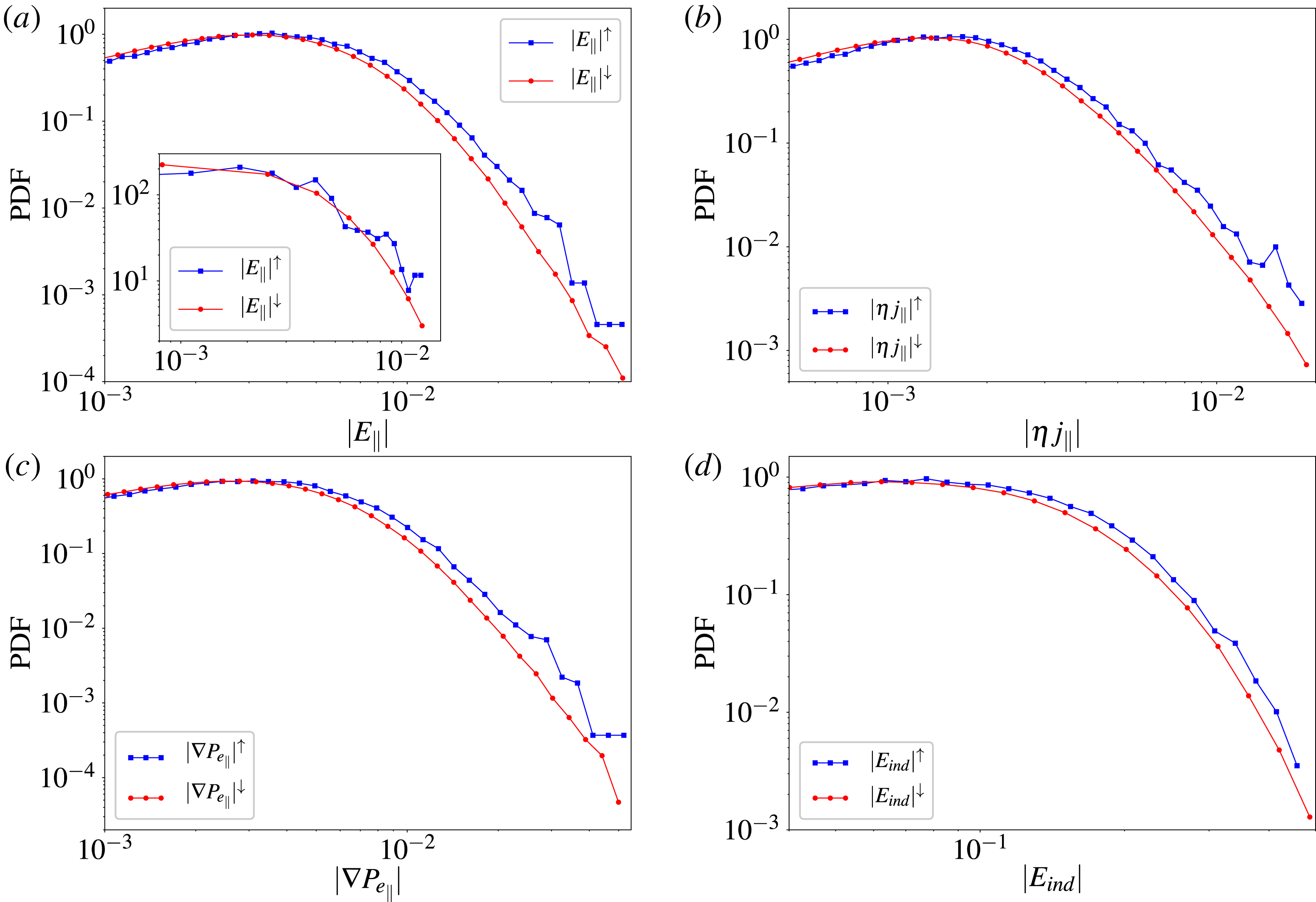
Conditional PDFs of the magnitudes of the individual contributions to the electric field (see (2.1)). In each case the condition is related to the particle acceleration. PDFs designated by
 $^{\uparrow }$
(blue squares) are the PDFs accumulated at positions of particles with anomalous acceleration, defined as particle with acceleration value exceeding
 $3\unicode[STIX]{x1D70E}$
in the global distribution of the particle accelerations. Likewise PDFs for the particles with normal acceleration, indicated by
 $^{\downarrow }$
(red circles), are accumulated at the positions of particles having acceleration less than
 $1\unicode[STIX]{x1D70E}$
. The four cases shown are the conditional distributions of magnitude of: (a) total parallel electric field
 $|E_{\Vert }|$
; (b) parallel resistive electric field
 $|\unicode[STIX]{x1D702}j_{\Vert }|$
; (c) parallel electron pressure
 $|\unicode[STIX]{x1D735}P_{e\Vert }|$
; and (d) total inductive electric field
 $|\boldsymbol{u}\times \boldsymbol{B}|$
. The parallel
 $\Vert$
components are defined relative to the local magnetic field vector. All cases show the same qualitative behaviour: particles with larger accelerations are more likely to be found where the electric field values are larger. This supports the idea that accelerating particles cluster close to regions where dynamical activity is occurring, notably along boundaries of interacting flux tubes, and near the associated current sheets, suggesting an association with magnetic reconnection. The inset of (a) shows the total parallel electric field component conditioned over the PVI values. The red circles are the parallel electric field values computed along the whole PVI path, whereas the blue squares are the parallel electric field values computed in the regions where the PVI exceeds a threshold value. This correlation indicates that high electric field values are more probable to be found where magnetic field inhomogeneities are stronger.

In order to establish a more quantitative link between the parallel electric field and possible local acceleration effects, we compared the PDFs of the separate contributions to the electric field (see (2.1)). We focus on those terms that can be parallel to the local magnetic field (namely
 $\unicode[STIX]{x1D735}P_{e}$
and
 $\unicode[STIX]{x1D702}j$
) and on the total parallel electric field itself (
 $E_{\Vert }$
), moreover we also examine the total inductive electric field
 $\boldsymbol{u}\times \boldsymbol{B}$
. To make an association with the acceleration of particles, we accumulate the PDFs of these quantities at particles positions, after dividing the particles into low-acceleration and high-acceleration populations. These populations were distinguished by thresholds with respect to the global acceleration PDF: the anomalous particles are those which have an acceleration value exceeding the
 $3\unicode[STIX]{x1D70E}$
of the global distribution, whereas ‘normal’ particles have an acceleration value within
 $1\unicode[STIX]{x1D70E}$
. Note that the above conditional statistics would give the same distribution only if acceleration and the fields are uncorrelated. These PDFs are shown in figure 10, where the quantities with superscript
 $^{\uparrow }$
are measured at the positions of anomalously accelerated ions, whereas the fields with superscript
 $^{\downarrow }$
are related to ‘normal’ particles. It is evident that anomalous particles are located where the fields have higher values – the population of the distribution is higher for bigger values of these fields. Moreover we used the partial variance of increments (PVI) method to find candidate regions likely to be identified as coherent structures. These structures contribute to non-Gaussian statistics and therefore to intermittency. The PVI time series is substantially defined as the normalized sequence of magnetic increments. By applying the PVI technique (Greco et al.
Reference Greco, Matthaeus, Servidio and Dmitruk2009b
), we found that the regions of bigger
 $E_{\Vert }$
occur in correspondence of magnetic discontinuities and not in smooth regions, as the PDF of
 $E_{\Vert }$
conditioned on PVI values shows in the inset of figure 10(a). In the figure we see that each of the electric field contributions are enhanced at the positions of high-acceleration particles, indicating that a variety of possible mechanisms, each associated with high levels of dynamical activity, are at work. The apparent strong response at high values of the parallel electric field contributions further confirm the relation between the parallel electric field and the acceleration mechanisms in 2.5-D turbulence.
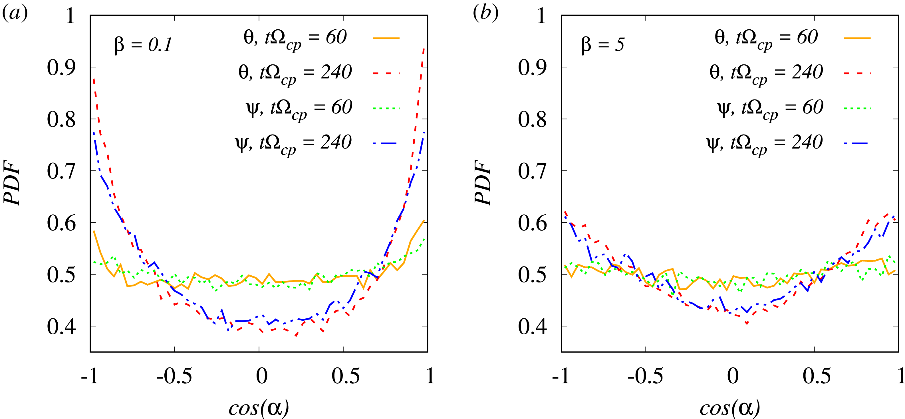
This acceleration mechanism in the out-of-plane direction has a global effect of elongating the ion velocity distribution function (VDF). In order to see if this typical alignment effect is present in our numerical experiments, we computed both the PDF of the angles between the particles’ velocity and the local magnetic field and the PDF of the angle the particles velocity forms with the main magnetic field (along
 $z$
)
 $$\begin{eqnarray}\displaystyle \cos (\unicode[STIX]{x1D703})=\frac{\boldsymbol{v}\boldsymbol{\cdot }\boldsymbol{B}}{|\boldsymbol{v}||\boldsymbol{B}|},\quad \cos (\unicode[STIX]{x1D713})=\frac{v_{z}}{|\boldsymbol{v}|}. & & \displaystyle\end{eqnarray}$$
In figure 11 we report the distributions of both these angles, at the initial and final times of the simulation, for different values of
 $\unicode[STIX]{x1D6FD}$
. At the initial time, when turbulence is very ‘young’, the distributions are quite flat, meaning particles are moving isotropically. As the simulation goes on, particles tend to align with the main magnetic field in the
 $z$
direction. This effects is much more evident for the low
 $\unicode[STIX]{x1D6FD}$
plasma, the more magnetized one. Another feature one can notice in the low
 $\unicode[STIX]{x1D6FD}$
plasma is that the particles orient themselves more on the local magnetic field rather than its
 $z$
component, although the
 $z$
component is its main one and the difference is not statistically relevant.
PDFs of the cosine of the angle between the particles’ velocity and the magnetic field for low (a) and high (b)
 $\unicode[STIX]{x1D6FD}$
values at the initial and at the final instants of the simulation. The orange (solid) and red (dashed) lines represent the PDFs of the angle the velocity forms with the local magnetic field at the initial and at the final time respectively. The green (dotted) and blue (solid-dotted) ones represent the angle that particles’ velocity forms with the main magnetic field in the
 $z$
direction at the same two instants. Both the two plasma scenarios start with an isotropic distribution of the velocities with respect to the magnetic field. Then the more magnetized particles (low
 $\unicode[STIX]{x1D6FD}$
plasma) become strongly aligned with the magnetic field. The same effect is evident, although much less pronounced, for the less magnetized particles (high
 $\unicode[STIX]{x1D6FD}$
plasma).

It is crucial to see now whether this acceleration mechanism, locally related to intense parallel electric fields, can actually increase the particles’ energy, and up to which values. This correspondence is not trivial since the particles with anomalous acceleration are only a small fraction of the plasma. We have built the energy PDF to see whether the energy has a different behaviour at different
 $\unicode[STIX]{x1D6FD}$
’s. The energy PDFs for the low and high
 $\unicode[STIX]{x1D6FD}$
values are shown in figure 12. In the low
 $\unicode[STIX]{x1D6FD}$
scenario the PDF develops a power law tail, already seen in observations and previous numerical simulations, whereas in the high
 $\unicode[STIX]{x1D6FD}$
plasma the energy remains similar to the initial distribution, namely close to the Maxwellian distribution. This suggests that the acceleration mechanism can energize particles, and that the process depends on the plasma
 $\unicode[STIX]{x1D6FD}$
.
PDF of the particles’ energy, for the high and low
 $\unicode[STIX]{x1D6FD}$
simulations, at different times. The high
 $\unicode[STIX]{x1D6FD}$
distribution does not change during the simulation, whereas the low
 $\unicode[STIX]{x1D6FD}$
particles have a substantial energy gain because of turbulence.

4.1 Magnetic trapping
We have seen that the acceleration mechanism involves the parallel electric field. However, there must be something else that makes this field energize particles only in the low
 $\unicode[STIX]{x1D6FD}$
plasmas. In figure 9 we have seen that the anomalous particles lie within (or in between) magnetic islands, in agreement with previous discussions. The acceleration mechanism evidently occurs in association with magnetic reconnection. Particles temporarily trapped inside small flux tubes or in the dynamically active region of larger flux tubes experience Fermi-like processes. In the regions close to current sheets, particles can experience nearly continuous first-order energization (Hoshino et al.
Reference Hoshino, Mukai, Terasawa and Shinohara2001; Drake et al.
Reference Drake, Opher, Swisdak and Chamoun2010; Haynes et al.
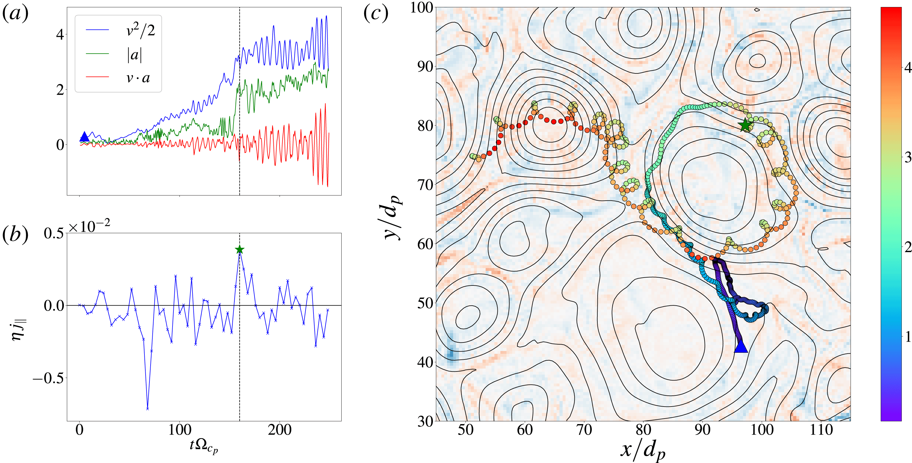
Reference Haynes, Burgess and Camporeale2014). In particular, we followed the trajectory of one of the most energetic particles and monitored its energy, its acceleration, the energy derivative with respect to time and the parallel current density it samples during its journey (the parallel pressure term is not shown because it is too noisy for non-statistical treatment) (figure 13). The figure also shows that the particle remains trapped in a magnetic island and its energy grows until it reaches a high enough value that allows the particle to escape.
One of the most energetic particles followed along its path. (a) Shows the particle energy (blue line), its acceleration (green line) and the energy time derivative (red line). (b) Shows the Lagrangian parallel current density, namely the value of
 $\unicode[STIX]{x1D702}j_{\Vert }$
measured along the particle trajectory. Both the energy and the acceleration show an increase in correspondence of a peak in the parallel current density. The energy and its time derivative are oscillatory, although there is a slightly positive component. After the energy boost the oscillation amplitudes grow, although the energy average value remains almost constant. This behaviour might be related to the sampling of a coherent field, until the particle becomes energetic enough to be free to escape. (c) Shows the colour map of the parallel electric field, at
 $t=160\unicode[STIX]{x1D6FA}_{cp}^{-1}$
, when the particle encounters the peak of the
 $\unicode[STIX]{x1D702}j$
term along its trajectory, with the particle path whose colour represents the particle’s energy. The colour clearly shows that the particle gets energized when it remains trapped in the magnetic island until it gets enough energy to escape. The (blue) triangle represents the starting point of the trajectory and the (green) star is the point where the maximum value of parallel current density is found.

To estimate the escape times we calculated the Lagrangian auto-correlation time using (4.4). This quantity represents the time during which each particle experiences a correlated field, and can be estimated as
 $$\begin{eqnarray}\displaystyle T_{\text{esc}}={\displaystyle \frac{1}{\langle v_{x}(t_{0})^{2}\rangle _{a}}}\int _{0}^{\infty }\langle v_{x}(t_{0})v_{x}(t_{0}+\unicode[STIX]{x1D70F})\rangle _{a}\,\text{d}\unicode[STIX]{x1D70F}. & & \displaystyle\end{eqnarray}$$
In the above definition, the operation
 $\langle \cdot \rangle _{a}$
is the average only over the particles that have high acceleration. For the usual isotropy hypothesis, we computed the above relation along all directions, finding similar results. We obtained the following escaping times:
 $T_{\text{esc}}^{\text{anom}}(\unicode[STIX]{x1D6FD}=5)\sim 0.8\unicode[STIX]{x1D6FA}_{cp}^{-1}$
,
 $T_{\text{esc}}^{\text{anom}}(\unicode[STIX]{x1D6FD}=0.5)\sim 3.0\unicode[STIX]{x1D6FA}_{cp}^{-1}$
and
 $T_{\text{esc}}^{\text{anom}}(\unicode[STIX]{x1D6FD}=0.1)\sim 5.7\unicode[STIX]{x1D6FA}_{cp}^{-1}$
. In addition we computed the same quantity for all the particles, obtaining these values:
 $T_{\text{esc}}^{\text{all}}(\unicode[STIX]{x1D6FD}=5)=0.95\unicode[STIX]{x1D6FA}_{cp}^{-1}$
,
 $T_{\text{esc}}^{\text{all}}(\unicode[STIX]{x1D6FD}=0.5)=4.13\unicode[STIX]{x1D6FA}_{cp}^{-1}$
,
 $T_{\text{esc}}^{\text{all}}(\unicode[STIX]{x1D6FD}=0.1)=9.64\unicode[STIX]{x1D6FA}_{cp}^{-1}$
. This scenario is consistent with the fact that particles in low
 $\unicode[STIX]{x1D6FD}$
plasmas develop high energy tails, since they are confined within magnetic islands for longer periods, experiencing the same parallel electric field. On the other hand, particles in high
 $\unicode[STIX]{x1D6FD}$
plasmas easily escape from magnetic islands and are not efficiently energized. The comparison of the trapping times values at the same
 $\unicode[STIX]{x1D6FD}$
for the different kinds of particle populations also supports this view. The escaping times calculated over all the particles are bigger than those of the anomalous particles, suggesting that more energetic particles are more likely to escape from magnetic islands while lower energy particles remain trapped for longer periods and can be coherently energized. This Fermi-like process, invoked in small-scale reconnection (Ambrosiano et al.
Reference Ambrosiano, Matthaeus, Goldstein and Plante1988), is now quantitatively observed in large-scale plasma turbulence. It is interesting now to further characterize the energization process by looking at the characteristic parameters of these anomalous particles.
4.2 The magnetic moment
We now further inspect the acceleration process by looking at the magnetic moment
 $\unicode[STIX]{x1D707}$
of ions, defined as
 $$\begin{eqnarray}\displaystyle \unicode[STIX]{x1D707}={\displaystyle \frac{mv_{\bot }^{2}}{2B}}. & & \displaystyle\end{eqnarray}$$
In the above expression,
 $m$
is the particle mass and
 $v_{\bot }$
its velocity (perpendicular to the magnetic field
 $\boldsymbol{B}$
, measured at the particle’s position). The magnetic moment is an adiabatic invariant of the system if the magnetic field is slowly varying. Indeed, in this case, the particles’ orbits are like closed circles and the flux of magnetic field passing through them is almost constant. This suggests that the magnetic moment might not be a constant of the motion in a turbulent system where several spatial scales are present, and where magnetic field variations are neither negligible nor adiabatic (Dalena et al.
Reference Dalena, Greco, Rappazzo, Mace and Matthaeus2012). To quantify the behaviour of the magnetic moment for each particle, we computed the normalized moment
 $$\begin{eqnarray}\displaystyle \tilde{\unicode[STIX]{x1D707}}_{p}={\displaystyle \frac{\unicode[STIX]{x1D707}_{p}(t)-\unicode[STIX]{x1D707}_{p}(0)}{\unicode[STIX]{x1D707}_{p}(0)}}, & & \displaystyle\end{eqnarray}$$
where the label
 $p$
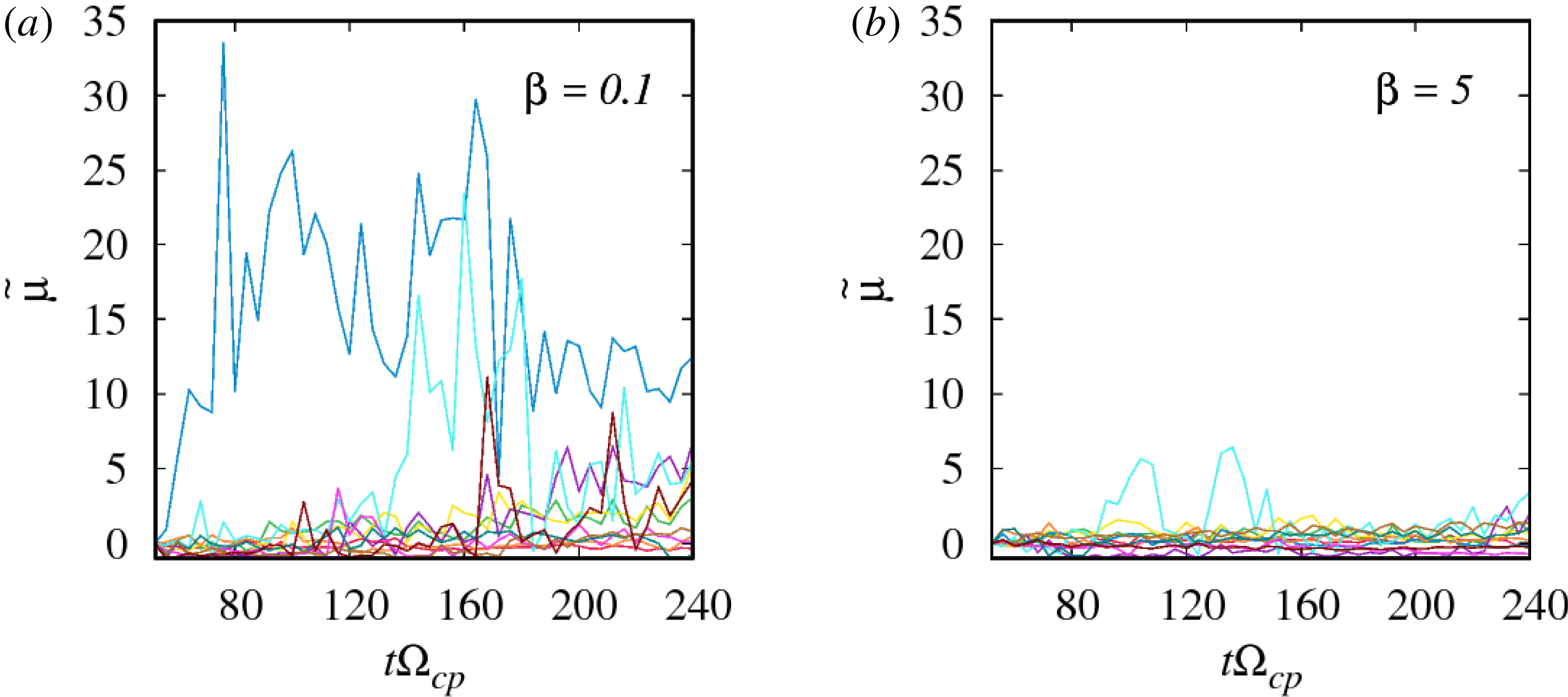
now indicates a single particle. This measure gives us information about the variation of the particle magnetic moment with respect to its initial value. Figure 14 shows
 $\tilde{\unicode[STIX]{x1D707}}_{p}$
as a function of time, for some particles, randomly selected, for two plasma
 $\unicode[STIX]{x1D6FD}$
values. Particles that moves in low
 $\unicode[STIX]{x1D6FD}$
plasma have the highest magnetic moment excursions, while in the high
 $\unicode[STIX]{x1D6FD}$
plasma, where particles are not so energized in time, their magnetic moment is much more conserved.
Magnetic moment as a function of time, for a group of 11 randomly selected particles, for two values of
 $\unicode[STIX]{x1D6FD}$
. The violation of magnetic moment conservation is much more pronounced in the case of
 $\unicode[STIX]{x1D6FD}=0.1$
, for which some particles experience great variations. In the low-
 $\unicode[STIX]{x1D6FD}$
plasma, particles have gyro-radii of the order of the local strong inhomogeneities’ dimensios with which they can probably interact, while in the high-
 $\unicode[STIX]{x1D6FD}$
plasma this interaction can not occur and particles’ magnetic moment is better conserved.

To see whether the magnetic moment is a constant of the motion, in a more quantitative way (figure 14 refers only to a small portion of particles), we calculated the standard deviation
 $\unicode[STIX]{x1D70E}_{\unicode[STIX]{x1D707}}(p)$
. This can be interpreted as the dispersion of the magnetic moment, for each particle, and is defined as
 $$\begin{eqnarray}\displaystyle \unicode[STIX]{x1D70E}_{p}=\sqrt{\frac{1}{T}\int _{t_{0}}^{t_{0}+T}[\unicode[STIX]{x1D707}_{p}(t^{\prime })-\langle \unicode[STIX]{x1D707}_{p}\rangle _{T}]^{2}\,\text{d}t^{\prime }}, & & \displaystyle\end{eqnarray}$$
where
 $\unicode[STIX]{x1D707}_{p}(t)$
is the magnetic moment of the
 $p$
th particle at the time
 $t$
, and the average in the integral is calculated over the whole time. In case of a perfectly conserved magnetic moment, this quantity is null. We have then built the PDF of
 $$\begin{eqnarray}\displaystyle \unicode[STIX]{x1D700}={\displaystyle \frac{\unicode[STIX]{x1D70E}_{p}}{\langle \unicode[STIX]{x1D707}_{p}\rangle _{t}}}, & & \displaystyle\end{eqnarray}$$
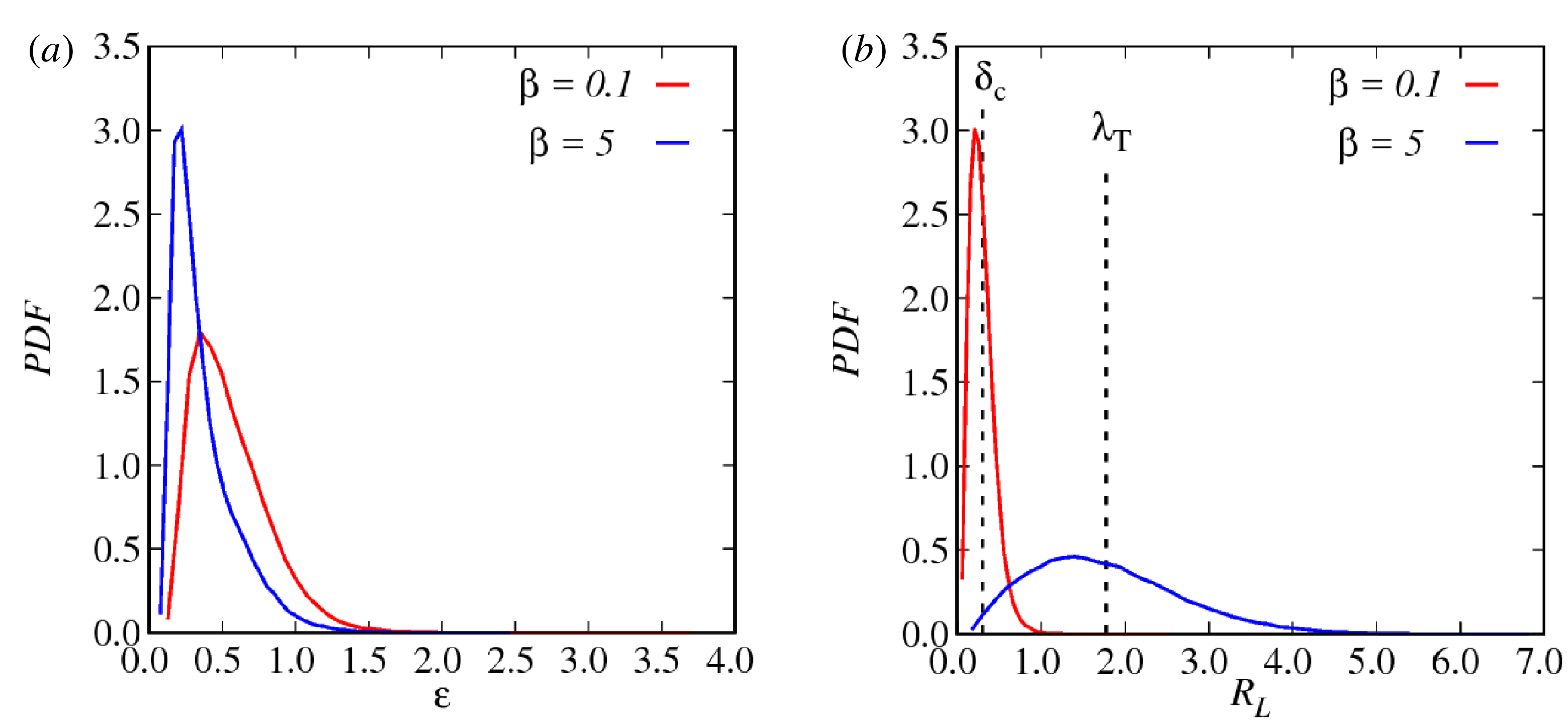
that indicates how much the magnetic moment deviates from its mean value – how much the magnetic moment is ‘broken’. The PDF
 $(\unicode[STIX]{x1D700})$
is shown in figure 15(a), for the whole
 $10^{5}$
particles. The violation of the magnetic moment is much more pronounced (broader distribution) in the case of
 $\unicode[STIX]{x1D6FD}=0.1$
. Low-
 $\unicode[STIX]{x1D6FD}$
particles have small gyro-radii and they can probably interact with the local strong inhomogeneities, while high-
 $\unicode[STIX]{x1D6FD}$
particles keep their magnetic moment better conserved.
(a) PDF of the dispersion of the magnetic moment defined in (4.8). These PDFs show that particles are more likely to ‘break’ their magnetic moment in the low
 $\unicode[STIX]{x1D6FD}$
case. (b) PDF of the Larmor radius for different
 $\unicode[STIX]{x1D6FD}$
values. High
 $\unicode[STIX]{x1D6FD}$
particles have a wide distribution, reaching values up to one order of magnitude bigger than in the low-
 $\unicode[STIX]{x1D6FD}$
case. The Taylor length
 $\unicode[STIX]{x1D706}_{T}$
and the current width
 $\unicode[STIX]{x1D6FF}_{c}$
are also indicated. The Taylor length indicates the length of the biggest current sheet in the plane and sets an upper limit to the particles that can effectively get energized by interacting with the current sheets. Whereas the current width
 $\unicode[STIX]{x1D6FF}_{c}$
is the average current sheet thickness.

We can relate the magnetic moment violation directly to the turbulence characteristic scales. Our analysis suggests that particles can interact with current sheets if their Larmor radius is much shorter than the Taylor length
 $\unicode[STIX]{x1D706}_{T}$
– the largest current sheet size (2.3). If the radius is bigger, the particle can gyrate without even ‘noticing’ the current sheets. The other important scale is the current sheets’ width
 $\unicode[STIX]{x1D6FF}_{c}$
, that is the mean size of the current sheet cores. Figure 15(b) shows a more quantitative view of the above speculation, suggesting a kind of spatial resonance. In this figure we report the PDF of the Larmor radius along with the turbulence characteristic lengths
 $\unicode[STIX]{x1D706}_{_{T}}$
and
 $\unicode[STIX]{x1D6FF}_{c}$
. The Larmor radii of particles in high
 $\unicode[STIX]{x1D6FD}$
plasma are broadly distributed and are much bigger than the current sheets’ thickness. The case with
 $\unicode[STIX]{x1D6FD}=0.1$
shows, instead, that the average
 $R_{L}$
are smaller than (or of the order of)
 $\unicode[STIX]{x1D6FF}_{c}$
. In this scenario, particles with the resonant Larmor radius feel the presence of the sharp discontinuities, and undergo a magnetic moment break. This eventually leads to the acceleration mechanism, and to the energization of ions in turbulent plasmas.
4.3 Approaching velocity-space diffusion
We have studied the processes of particle acceleration and energization. Acceleration can be interpreted as ‘motion’ in velocity space, i.e.
 $v$
-diffusion (Subedi et al.
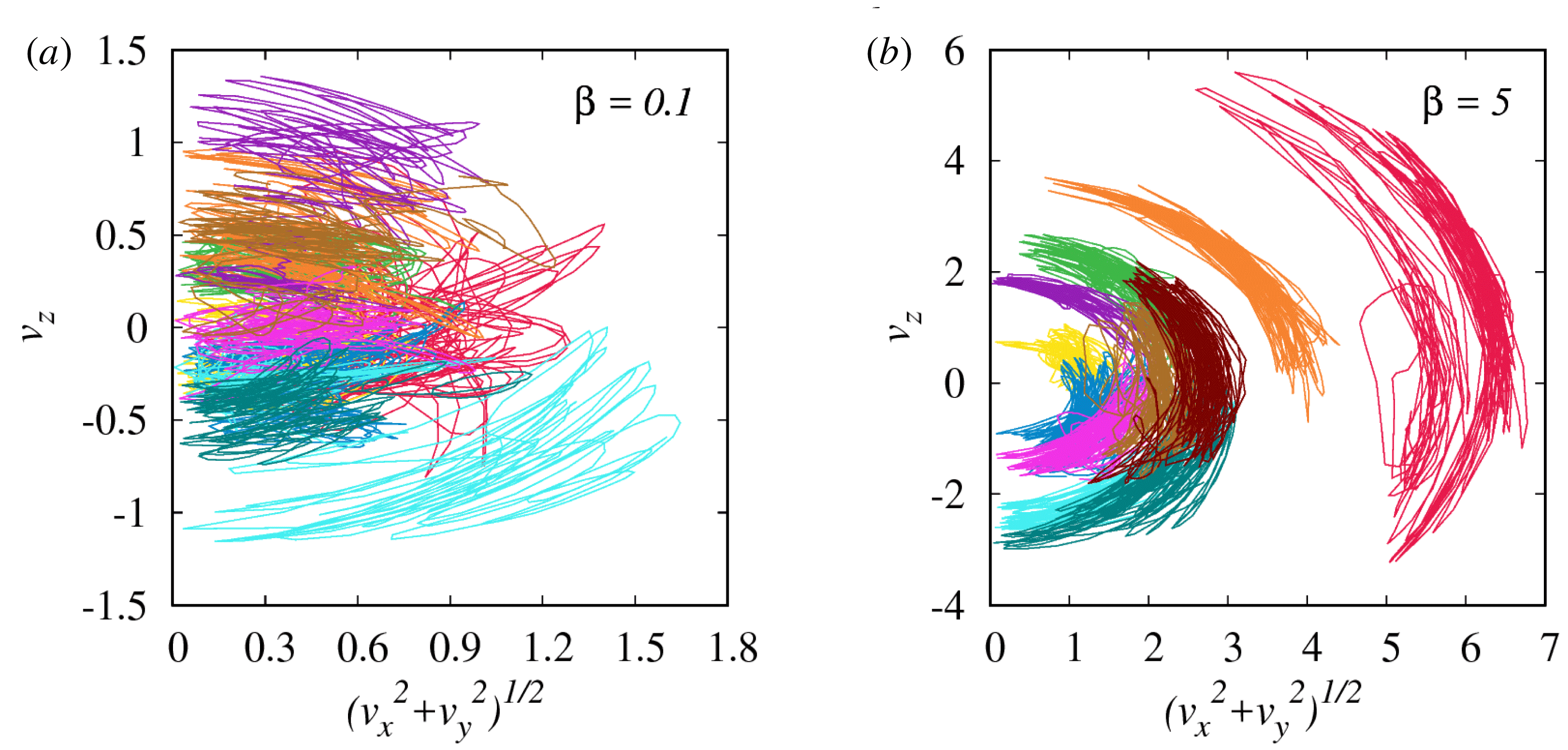
Reference Subedi, Sonsrettee, Blasi, Ruffolo, Matthaeus, Montgomery, Chuychai, Dmitruk, Wan and Parashar2017). In this last section we will briefly mention this aspect of diffusion. As for spatial diffusion, it is instructive to observe particles’ trajectories, now in the velocity space. In particular, we represent these trajectories in a 2-D space made by
 $v_{z}$
(parallel to the global magnetic field) and the in-plane velocity
 $(v_{x}^{2}+v_{y}^{2})^{1/2}$
. The trajectories in the velocity space are shown in figure 16.
Velocity-space trajectories for the same particles of figure 14, at high and low
 $\unicode[STIX]{x1D6FD}$
values. Particles moving in the high
 $\unicode[STIX]{x1D6FD}$
plasma are more energetic and do not undergo an energization processes. They diffuse in pitch angle and hence move on quasi-isoenergetic shells. Differently, in the low
 $\unicode[STIX]{x1D6FD}$
scenario, particles manifest more complex (ergodic) trajectories: they are not locked on isoenergetic shells as they can effectively gain/lose energy through their journey across magnetic islands.

The velocity-space trajectories show, from another point of view, the same behaviour we have seen in the previous sections. In the high
 $\unicode[STIX]{x1D6FD}$
plasma, particles are accelerated but not effectively energized by the parallel electric field. This means that they can diffuse only in pitch angle and gyrophase, namely they move on the surface of isoenergetic shells, varying only the angle the velocity forms with the magnetic field. In the low
 $\unicode[STIX]{x1D6FD}$
scenario, particles, instead, are accelerated and decelerated by the current sheets and the islands (note, however, that the percentage of high energy particles is very low). The combined acceleration, deceleration and energization phenomena make the particles’ trajectories in the velocity space more complex, almost ergodic, since particles can diffuse both in pitch angle and momentum amplitude. The ergodicity domain is bounded by the upper limit of the energy a particle can gain before escaping a vortex and run into a decelerating (de-energizing) electric field. This interesting aspect of velocity diffusion will be further inspected in future works.
5 Discussion and conclusions
In this work we described the diffusion and the acceleration of ions in plasma turbulence using self-consistent hybrid simulations (kinetic ions and fluid electrons). These topics are of primary importance both in astrophysical and laboratory plasmas. We simplified the problem by using a 2.5-D geometry, which can be a valid approximation to understand the nature of strongly anisotropic (magnetized) fluctuations (Shebalin, Matthaeus & Montgomery Reference Shebalin, Matthaeus and Montgomery1983; Matthaeus & Lamkin Reference Matthaeus and Lamkin1986; Dmitruk, Matthaeus & Seenu Reference Dmitruk, Matthaeus and Seenu2004). Particles have been evolved making use of a PIC algorithm. The PIC algorithm is very useful and of practical fundamental importance when treating non-equilibrium plasmas for which the wave–particle interactions are crucial. The 2.5-D hybrid-PIC simulations have been performed for three different
 $\unicode[STIX]{x1D6FD}$
values, in order to reproduce a wide range of physical systems. The different values of
 $\unicode[STIX]{x1D6FD}$
used vary for more than one order of magnitude allowing us to describe plasma scenarios spanning from the solar corona to fusion devices. The 2-D maps of the current density along with the magnetic field showed the development of fundamental turbulent structures, such as vortices and current sheets.
We have then studied the motion of ions, moving self-consistently in the electromagnetic field. As suggested by previous (and numerous) test-particle studies, the motion is very erratic. Particles can be trapped in magnetic vortices or scattered by current sheets, wandering like pollen in the atmosphere (Servidio et al. Reference Servidio, Haynes, Matthaeus, Burgess, Carbone and Veltri2016), or field lines in the solar corona (Rappazzo et al. Reference Rappazzo, Matthaeus, Ruffolo, Velli and Servidio2017). These kinds of trajectories are achieved after rather long time intervals and can be statistically described within the theory of diffusion. The particle motion becomes uncorrelated when the particle is no longer trapped by the same vortex. Low energy particles have been found to have longer correlation times as they cannot easily escape from vortices.
All the existing theories on the diffusion coefficient can describe 3-D systems and all these theories have been verified only with test-particle models. The NLGC theory is possibly the most precise theory that gives an estimate of the diffusion coefficient. We have then ‘reduced’ this theory to the bi-dimensional case. This 2-D NLGC theory has been found to be valuable in describing the diffusion coefficient of particles moving in self-consistent turbulent fields.
From the acceleration process, the PDFs show that the nature of the acceleration depends on the plasma
 $\unicode[STIX]{x1D6FD}$
. Acceleration is a stochastic variable for the high
 $\unicode[STIX]{x1D6FD}$
plasmas, whereas it is distributed with power-law tails for the low
 $\unicode[STIX]{x1D6FD}$
cases. We have found that the electric field component parallel to the magnetic field is correlated with particle acceleration. The ‘anomalously’ accelerated particles, i.e. the particles with acceleration values that exceed the variance of the distribution, are connected to the regions where the parallel electric field is more intense. This has been seen, qualitatively, by spotting these particles on the parallel electric field map and, quantitatively, by computing the conditional statistics. It is worth noting that only a small percentage of particles is affected by the acceleration mechanism. Therefore, this result is consistent with the free streaming of average out of plane speeds, described in figure 5. The acceleration is more efficient in the perpendicular plane (not shown here).
By looking at the energy PDFs, we noticed that particles in low
 $\unicode[STIX]{x1D6FD}$
systems, such as in the solar wind, are more effectively energized. This process can be linked to the presence of narrow current layers. The main phenomenon acting on the particle is the breaking of the magnetic moment. Local spatial resonances break this constant of the motion, leading to acceleration and eventually to energization. In this process the particles undergo a spatial resonance with the background turbulent structures: ions that have a Larmor radius of the order of the current sheet thickness experience large excursions of their magnetic moment. These particles experience a local acceleration process, while in the case with much larger
 $\unicode[STIX]{x1D6FD}$
, as can be found in the magnetospheric environment, the plasma elements do not ‘see’ the reconnecting current sheets and the embedded parallel electric field. This kind of interaction with vortices and current sheets has been shown also by looking at resonances between characteristic scales. The particles’ characteristic scale is the Larmor radius, whereas for turbulence we computed the Taylor length and the current sheets’ cores average width. A consistent percentage of high energy particles have a Larmor radius bigger than the Taylor length, that is, qualitatively, the in-plane length of the biggest current sheet. This means that high energy particles barely notice the current sheets.
Finally, we have introduced the concept of velocity-space diffusion because the above processes might be related to the stochastic motion of the particles in the velocity space. We still lack a fundamental theory to determine the diffusion coefficient in velocity space (Miller, Guessoum & Ramaty Reference Miller, Guessoum and Ramaty1990; Miller & Roberts Reference Miller and Roberts1995), and we leave this work for future studies. Future works can be focused on an analytical treatment of the velocity-space diffusion. Moreover, a full 3-D study will be performed, taking into account also the role of kinetic electrons.
To conclude, it would be very interesting to highlight the main effects on diffusion and acceleration due to the self-consistent (kinetic) treatment of particles, performing, for example, a direct comparison with MHD test-particle simulations, with the same numerical setting presented here. We will investigate these issues in future work.
Acknowledgements
This work is partly supported by the International Space Science Institute (ISSI) in the framework of International Team 405 entitled ‘Current Sheets, Turbulence, Structures and Particle Acceleration in the Heliosphere’, by the US NSF AGS-1156094 (SHINE) and by NASA grant NNX14AI63G (Heliophysics Grandchallenge Theory), the MMS mission through grant NNX14AC39G, and the Solar Probe Plus science team (ISOIS/Princeton subcontract SUB0000165).