

Introduction
Aflatoxin is a mycotoxin produced by Aspergillus flavus or Aspergillus parasiticus fungi. Aflatoxin contamination of food is a worldwide problem (Liu and Wu, Reference Liu and Wu2010) because it can cause liver cancer in humans and animals (Barrett, Reference Barrett2005). Therefore, the identification of aflatoxin risk areas can help prevent contamination. Aflatoxin contamination is mostly driven by high temperatures and drought conditions (Patriaca et al., Reference Patriarca, Medina, Pinto and Magan2014; Payne, Reference Payne1992) so if high risk areas are known prior to planting, farmers can adapt management practices to the conditions in the area. Specific strategies can be employed before planting by adapting seeding rate or type of corn hybrid, during growth by using variable rate irrigation and modified irrigation scheduling, or at harvest by segregating areas with different levels of risk.
The aflatoxin risk for corn fields in south eastern USA is high because of rainfall variability and extreme heat events which occur in the region and are exacerbated where soils are light textured (Widstrom et al., Reference Widstrom, Forster, Martin and Wilson1996). Aflatoxin assessment requires the collection of multiple corn samples, it is expensive (Papadoyanis, Reference Papadoyanis1990) and conducted at harvest which does not allow implement of in-season adaptation strategies to reduce the risk. Given the cost of aflatoxin analysis, one role of extension services in precision farming is to identify the areas most at risk of contamination so that farmers can know if altering management strategies is worthwhile. Kerry et al. (Reference Kerry, Ortiz, Ingram and Scully2017) developed a risk factors approach to determining contamination risk which was verified using 30 years spatio-temporal summary of aflatoxin risk produced by Poisson kriging of county level data for southern Georgia. The approach used the following risk factors which have been identified as important to contamination risk: June maximum temperatures (Salvacion et al., Reference Salvacion, Ortiz, Scully, Wilson, Hoogenboom and Lee2011), June rainfall (Salvacion et al., Reference Salvacion, Ortiz, Scully, Wilson, Hoogenboom and Lee2011), percentage of well and excessively drained soils (Palumbo et al., Reference Palumbo, O’Keeffe, Kattan, Abbas and Johnson2010; Damianidis et al., Reference Damianidis, Ortiz, Windham, Scully and Woli2015), percentage of area in corn production. The contamination risk was determined based on the number of risk factors that were above key thresholds. The approach was developed as a county level study, however, knowing of smaller areas which are more specifically at risk would be helpful in determining appropriate management strategies. Kerry et al. (Reference Kerry, Ortiz, Ingram and Scully2017) mentioned that data could be kriged to a dense grid to get an idea of within county variations in risk factors and aflatoxin risk, however, real data for individual seasons, regarding actual crop response to these risk factors would be the ideal way to determine risk.
NDVI data from remotely sensed images indicate the greenness of vegetation and have been used to indicate variations in crop health and yield within fields (Hatfield and Prueger, Reference Hatfield and Prueger2010; Wang et al., Reference Wang, Cherkauer and Bowling2016) in response to differences in water supply and nutrients. Thermal infra-red data have also been used to indicate drought stress (Jones et al., Reference Jones, Serraj, Loveys, Xiong, Wheaton and Price2009, Sepúlveda-Reyes, Reference Sepúlveda-Reyes, Ingram, Bardeen, Zúñiga, Ortega-Farías and Poblete-Echeverría2016). The current research expands on the methodology of Kerry et al. (Reference Kerry, Ortiz, Ingram and Scully2017) to try to define ‘high risk’ areas at the sub-county level. This is done by examining correlations with NDVI and thermal IR data for kriged and actual values of other risk factors in the corn producing area for 2011, a high risk year.
Materials and methods
Several layers of data were included in this analysis for southern GA. Two scales, county level and a 1 km grid, were examined. Details of how data were collected and processed are given below.
Weather Information
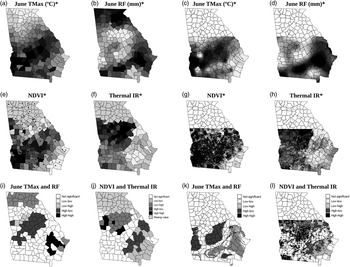
Monthly weather data for each year 1977–2004 were extracted from the Georgia Weather Network (http://georgiaweather.net). Weather station locations are shown in Figure 1e as black dots. June maximum temperatures (°C, June TMax) and June rainfall (mm, June RF) were ordinary kriged to county centroids and to a 1 km grid.
Maps of GA at the county (a-b, e-f, j-k) and 1 km grid scale (c-d, h-I, l-m) showing: June TMax (a, c), June RF (b, d), NDVI (e, h), Thermal IR (f, i) and Local Moran’s I analysis of drought affected zones (j-m). *maps with no legend are plotted as deciles - white areas are low values and black high

Corn Production Area
The locations where corn was grown were extracted from http://nassgeodata.gmu.edu/CropScape/ for the 2011 growing season. These 30 m pixel data were then used to determine the percentage area of each county and 1 km grid square in corn production.
Soil Information
Excessively and well drained soils were identified from a geo-corrected soil association map (1:250,000, NRCS, 2006). Based on the pixels within each county identified as being in corn production in the 2011 CropScape image, the percentage of the crop growing area in each county and 1 km grid square with well and excessively drained soils was calculated.
NDVI
Multi-band imagery from the second half of June 2011 available in the Landsat Thematic Mapper (TM) dataset were downloaded from https://earthexplorer.usgs.gov. They were geo-corrected and stitched together to create a large image covering southern GA. The NDVI was then calculated for each pixel in the corn growing area based on the 2011 CropScape image. Thermal IR data was also extracted. The quality assessment band was used to ensure that any pixels covered by cloud were discarded. The average NDVI and thermal IR values of corn growing, cloud free pixels were then calculated for each county and 1 km grid square.
Risk Factors Approach
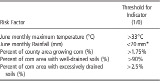
Information from each data layer was transformed into indicators based on the thresholds given in Table 1. Thresholds for June Tmax and June RF were chosen with respect to 30-year normal Tmax and RF in the area to show hotter and drier years than normal. Thresholds for the other risk factors were determined based on tails of the distribution of data in histograms. The indicators were then summed and counties and 1 km grid squares with summed indicator scores ≥3 were considered high risk.
Threshold values used for Risk Factor Indicators

* 50 mm used for other years by Kerry et al. (Reference Kerry, Ortiz, Ingram and Scully2017)
Statistical Analysis
A bivariate adaptation of the local Moran’s I (Anselin, Reference Anselin1995) was used to identify statistically significant (p=0.05) clusters in the weather and remotely sensed data. Two rings of queen neighbours were used as the moving window size for the county level data and the nearest 24 points for the 1 km grid data. High-high (HH) and Low-low (LL) clusters show areas where the first and second variables both have significant (p=0.05) clusters with high values or low values, respectively compared to a null hypothesis of spatial randomness. This indicates positive correlation between the variables and significant spatial autocorrelation in each of the variables. High-low (HL) clusters show areas where the first variable has high values and the second low and the converse is true for Low-high (LH) clusters. This shows negative correlation between the two variables but significant (p=0.05) positive spatial autocorrelation in each of the variables.
Results and Discussion
Kerry et al. (Reference Kerry, Ortiz, Ingram and Scully2017) showed through a Poisson kriged 30 year spatio-temporal summary of corn aflatoxin contamination in southern GA that the areas with the greatest proportion of years with aflatoxin levels over the FDA 20 ppb contamination threshold were in the centre and north of the area. This could be used to identify high risk areas before planting to adapt planting strategies, but is not useful for determining if an area will be at high risk in an individual season. The high risk areas identified by Poisson kriging (Kerry et al., Reference Kerry, Ortiz, Ingram and Scully2017) largely corresponded with the areas where June RF was below and June TMax was above the thresholds given in Table 1. Here, NDVI and thermal IR data of the corn growing area are used to indicate the crop response to weather conditions in the 2011 growing season at the county and 1 km grid level. If both scales illustrate similar patterns, it should be possible to use such data to identify areas at high risk of contamination at the sub-county level. Figure 1a and c show June TMax at the county and 1 km grid scales. Both show high temperatures in a swath across the central part of southern GA from the south west to the north east corners, with lower TMax values surrounding this swath. The average NDVI values for the county and 1 km grid data (Figure 1 e and h) largely show the same pattern as June TMax suggesting that the variables are positively correlated. Pearson correlation coefficients between June TMax and NDVI were r=0.49 and 0.39 (p<0.01) for the county and 1 km grid data, respectively.
Figure 1 b and d show June RF at the county and 1 km grid scales. Both show low rainfall totals in the north west of the region and high rainfall in the south east. The average thermal IR values for the county and 1 km grid data (Figure 1 f and i) largely show the opposite patterns to rainfall data with high values in the northwest and high in the south east. The similarity in patterns suggests these data are negatively correlated. Pearson correlation coefficients between June RF and thermal IR were r=−0.60 and −0.48 (p<0.01) for the county and 1 km grid data, respectively.
Given the correlations between June TMax and NDVI and June RF and thermal IR these data were used in Local Moran’s I analysis to identify the drought prone areas. Figure 1 j and l show the drought prone areas as High-low (HL) clusters, these are statistically significant clusters of high June TMax and low June RF. Figure 1 k and m show the drought prone areas as Low-high (LH) clusters as identified by the Local Moran’s I analysis of the NDVI and thermal IR data. One would expect crops experiencing drought stress to have low NDVI values and high thermal IR values. The drought prone areas identified by local Moran’s I analysis of weather and the remotely sensed data largely correspond and are found in the central north to northwestern part of the study area.
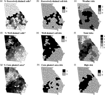
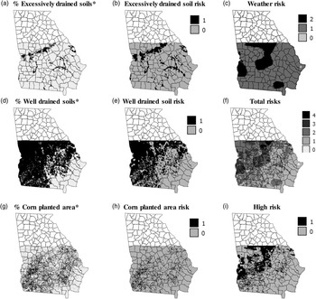
The distribution of excessively drained soils, well drained soils and corn planted area are shown at the county (Figure 2 a, d, g) and 1 km grid scales (Figure 3 a, d, g). These risk factors modify the influence of drought\aflatoxin risk compared to looking at weather alone. The actual distribution of drought as displayed in remotely sensed imagery (Figure 1 k and m) should more closely resemble the patterns in total risk as shown in Figure 2 and 3 f rather than the pattern in weather alone (Figures 2 and 3 c). Assuming that the clusters identified by local Moran’s I analysis of NDVI and thermal IR are a more accurate reflection of the actual drought stress in corn plants in 2011 than weather pattern alone, one would expect a greater percentage agreement between these Moran’s I results and the high risk areas identified with the risk factors approach when including all variables than when only weather data were used. The percentage agreement with the remotely sensed Moran’s I classification based on weather data alone was 100% at the county scale and 38% at the 1 km scale agreement whereas when all risk factors were included the percentage agreement was 57% at the county scale and 44% at the 1 km scale. This suggests that at the county scale average NDVI and Thermal IR data reflect the weather patterns whereas at the 1 km scale factors such as soil drainage are also important. This makes the case for future studies using remotely sensed data to help assess aflatoxin contamination within individual fields that have marked textural differences and are found in the high risk zones identified here.
Maps at the county scale showing percent coverage and risk from: excessively drained soil (a-b), well drained soil (d-e) and corn planted area (g-h). Weather risk (c), total number of risks (f) and high risk counties (i). *maps with no legend are plotted as deciles - white areas are low values and black high

Maps at the 1km grid scale showing percent coverage and risk from: excessively drained soil (a-b), well drained soil (d-e) and corn planted area (g-h). Weather risk (c), total number of risks (f) and high risk counties (i). *maps with no legend are plotted as deciles - white areas are low values and black high

Conclusions
This research has shown that the risk factors approach of Kerry et al. (Reference Kerry, Ortiz, Ingram and Scully2017) identifies similar areas as at risk of aflatoxin contamination to NDVI and thermal IR data combined. The latter have the advantage of not being interpolated and reflecting actual crop response. Data for the risk factors approach and NDVI and thermal IR data are available within the growing season so using them together or alone to determine the most at risk locations in a given season is likely to be more useful than using the Poisson kriged space-time summary of Kerry et al. (Reference Kerry, Ortiz, Ingram and Scully2017) which can only assist with determining planting strategies by location. Identifying the locations where the risk factors approach and remotely sensed data both suggest high risk using data for the current season can identify the places most at risk and where in season and harvesting strategies may need to be adapted to deal with aflatoxin contamination. It would be useful to further verify this approach in one or two seasons with a costly state wide aflatoxin survey. The greater agreement with the Moran’s I analysis of the remotely sensed data for all risk factors rather than just weather data at the 1 km grid scale shows the importance of risk factors other than weather at the sub-county scale. It also shows that weather is important to investigate at the county scale. Future research could extend this work to focus on individual high risk counties and individual high risk fields with large variations in soil texture to determine more precise strategies to deal with aflatoxin contamination within fields.
Acknowledgements
This work was funded by NOAA RISA grant: NA10OAR4310215 and USDA-NIFA grant 2011-67003-30347. Thanks to Drs. D. Wilson, (University of GA), N. Widsrom (USDA-ARS), W. Wiseman (USDA-ARS) and K. Kreamer for data collection and support.