Principle of electrically small antennas

According to the definition, the size of an ESA is much smaller compared to the wavelength $\lambda$ and can be defined as [Reference Wheeler22]:

(1)\begin{equation}ka = \frac{2\pi}{\lambda} a \lt 1,\end{equation}

where $a$ is the radius of a sphere (also called the radiansphere) enclosing the antenna, and $k$ is the wavenumber. Based on (1), the equation defining the fractional bandwidth ( $B_\mathrm{frac}$) of the antenna is:

(2)\begin{equation}B_\mathrm{frac}=\frac{S-1}{Q_\mathrm{min}\sqrt{S}},\end{equation}

where $S$ is the standing wave ratio and the minimum $Q$ value ( $Q_\mathrm{min}$) is:

(3)\begin{equation}Q_\mathrm{min} = (ka)^{-3}+(ka)^{-1}.\end{equation}

This expression is the well-known Chu–Harrington limit [Reference Chu21, Reference Hansen23, Reference McLean24].

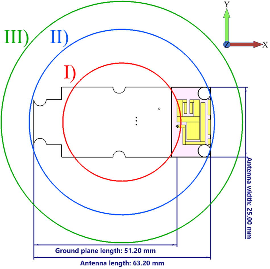
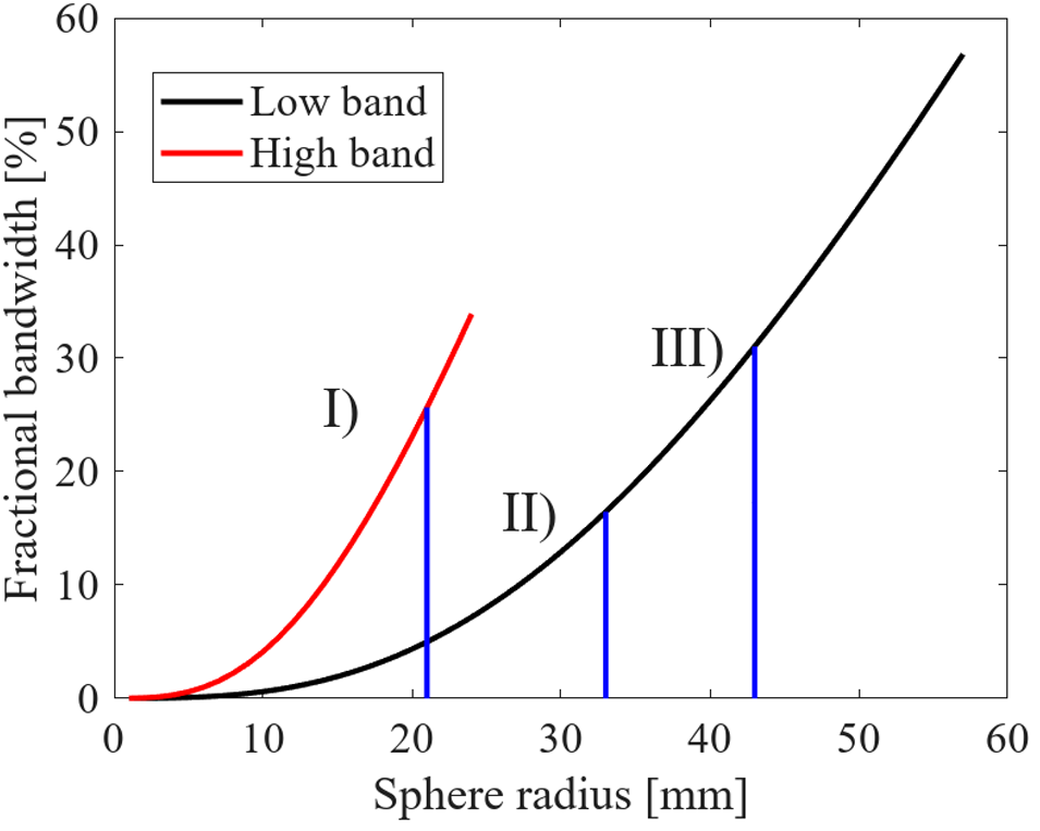
In this work, a challenging set of limits has been defined for the antenna due to the compactness of the device, as shown in Fig. 1. Different spherical radii calculated using (1)-(3) are visualized in the two-dimensional $xy$ plane, and the area allocated for the antenna placement is highlighted in pink. Note that the vertical area of the spheres cannot be utilized due to the geometrical constraints of the device. On the other hand, the expected fractional bandwidth ( $Bw$) limitations for the radii of Fig. 1 are plotted in Fig. 2. When estimating the $Bw$, the low band frequency is calculated based on $S_{lb}$ = 3 at $f$ = 830 MHz, and the high band case uses $S_{hb}$ = 2 at $f$ = 1.95 GHz. The plotted red and black lines in this figure highlight the electrically small regions for the high and low bands, respectively. It is worth noting that the ESA limit in the high band is at $a$ = 24 mm, which is slightly smaller than the size of the design. Despite not being considered electrically small at the high band (with $ka_{hb}$ = 1.35), a contrary and challenging condition exists at the low band (with $ka_{lb}$ = 0.57).

Figure 1.

Visualization of the different enclosing spheres with radius $a$ according to (1). Area allocated for the antenna design is highlighted in pink. The major dimensions of the PCB are annotated.

Figure 1 Long description

Different enclosing spheres around a printed circuit board are illustrated, highlighting dimensions relevant to antenna design. Three spheres are depicted, labeled as I, II and III, with I being the innermost and III the outermost. The innermost sphere is marked in red, the middle sphere in blue and the outermost sphere in green. The PCB is shown in the center, with specific dimensions annotated: the ground plane length is 51.20 millimeters and the antenna length is 63.20 millimeters. The distance width is noted as 25.29 millimeters. An axis indicator is present at the top right, showing the x, y and z directions. The area allocated for the antenna design is highlighted and the major dimensions of the PCB are clearly marked. The spatial arrangement and size considerations for the antenna design on the PCB are visually represented.

Figure 2.

ESA bandwidth limits calculated using eq. (1) in comparison to the enclosing sphere radius $a$. The markers indicate the following cases: I) Size required for high-band operation: $a$ = 21 mm / $Bw$ = 26%. II) Size of the design: $a$ = 33 mm / $Bw$ = 16%. III) Size required for low band operation: $a$ = 43 mm / $Bw$ = 31%.

Due to the narrow bandwidth available from ESAs, achieving instantaneous and wide bandwidth is very challenging. To widen bandwidth, multiple resonating structures that operate in complementary, closely-spaced bands could be implemented, similar to the technique in [Reference Koutinos, Zekios, Georgakopoulos and Kyriacou25]. However, due to the limited space available in this device, such a technique is not a viable option. Instead, enabling multiband operation using a switching element is a more realistic alternative. Switches do not require a large footprint, but enable the switched operation of the antenna resulting from multiple matching networks [Reference Garcia, Andújar, Pijoan and Anguera17]. This, in turn, allows the antenna to operate over the wider targeted bandwidth of operation when switching across closely-spaced bands. In this paper, the number of states is kept small (two) to keep the control circuitry manageable.

In practice, the band-switchable antenna system is a concept intended for the Bittium Faros^TM series of wearable cardiac monitors [26]. This requires the antenna section to be accommodated in an area of 14 $\times$25 mm $^2$ (0.04 $\times$0.07 $\lambda^2$) (area highlighted in pink). Besides that, it is assumed that the feed line and lumped components will be integrated within the same area as other circuits (printed circuit board areas in white in Fig. 1). These aspects will be explained in more detail in the following subsections.

Characteristic mode analysis

Characteristic mode analysis is an efficient tool to analyze the potential performance of an antenna design. It provides insight into the possible modes excited on a structure at a given frequency, allowing a more analytical path to identify the most suitable feed locations [Reference Martens, Safin and Manteuffel27, Reference Cabedo-Fabres, Antonino-Daviu, Valero-Nogueira and Bataller28].

To have an initial idea of the potentially available characteristic modes from the structure based on the lowest targeted frequency of 900 MHz, a series of characteristic mode analyses is first performed with varying ground plane sizes. When the ground plane is scaled to 150, 200, and 250% of the nominal size, the size of the antenna element remains constant in all cases. The modal significance of the first four characteristic modes at 900 MHz, when the ground plane size is increased in both axial dimensions (x and y), is shown in Fig. 3. It can be observed that the set physical size limitation (100%) of the device significantly restricts the availability of significant modes for antenna radiation. As the device size is increased, more modes become significant at the lower frequencies, with selected modes retaining their operation at the 1.7 GHz band.

Figure 3.

The change in modal significance of the first four characteristic modes at 900 MHz: a) Mode 1, b) Mode 2, c) Mode 3, and d) Mode 4, when the ground plane size is increased. The size of the ground plane (white) in Figure 1, was increased by 50% (red), 100% (green), and 150% (magenta), in both the x and y directions, whereas (blue) is the reference size. The different mode currents can be seen in Figure 4.

Figure 3 Long description

A line graph with the vertical axis labeled, Modal significance, ranging from 0 to 1 and the horizontal axis labeled, Frequency, with unit gigahertz, ranging from 0.5 to 2.5. A legend labeled, Scale, lists 100 percent, 150 percent, 200 percent and 250 percent. The 100 percent series uses a solid line. The 150 percent series uses a solid line. The 200 percent series uses a solid line. The 250 percent series uses a solid line. 100 percent: (0.5, 0.15), (0.6, 0.20), (0.7, 0.30), (0.8, 0.45), (0.9, 0.65), (1.0, 0.90), (1.1, 0.75), (1.2, 0.95), (1.3, 0.98), (1.5, 0.99), (2.0, 1.00), (2.5, 1.00). 150 percent: (0.5, 0.90), (0.6, 0.98), (0.7, 1.00), (1.0, 1.00), (1.5, 1.00), (2.0, 1.00), (2.5, 1.00). 200 percent: (0.5, 0.95), (0.6, 0.99), (0.7, 1.00), (1.0, 1.00), (1.5, 1.00), (2.0, 1.00), (2.5, 1.00). 250 percent: (0.5, 0.98), (0.6, 1.00), (0.7, 1.00), (1.0, 1.00), (1.5, 1.00), (2.0, 1.00), (2.5, 1.00). Key features in image A: 100 percent rises from 0.15 at 0.5 gigahertz to 0.90 at 1.0 gigahertz, dips to 0.75 at 1.1 gigahertz, then reaches 0.95 at 1.2 gigahertz and stays at 0.98 or higher from 1.3 to 2.5 gigahertz. 150 percent, 200 percent and 250 percent are at 0.90 or higher at 0.5 gigahertz and reach 1.00 by 0.7 gigahertz. The image B showing a line graph with the vertical axis labeled, Modal significance, ranging from 0 to 1 and the horizontal axis labeled, Frequency, with unit gigahertz, ranging from 0.5 to 2.5. The legend labeled, Scale, lists 100 percent, 150 percent, 200 percent and 250 percent. The 100 percent series uses a dotted line. The 150 percent series uses a dotted line. The 200 percent series uses a dotted line. The 250 percent series uses a dotted line. 100 percent: (0.5, 0.05), (0.6, 0.10), (0.7, 0.20), (0.8, 0.35), (0.9, 0.55), (1.0, 0.70), (1.1, 0.80), (1.2, 0.90), (1.3, 0.95), (1.5, 0.98), (1.7, 0.85), (1.9, 0.75), (2.1, 0.95), (2.3, 0.98), (2.5, 0.99). 150 percent: (0.5, 0.30), (0.6, 0.55), (0.7, 0.75), (0.8, 0.90), (0.9, 0.97), (1.0, 0.99), (1.5, 1.00), (2.0, 1.00), (2.5, 1.00). 200 percent: (0.5, 0.60), (0.6, 0.80), (0.7, 0.92), (0.8, 0.98), (0.9, 1.00), (1.0, 1.00), (1.5, 1.00), (2.0, 1.00), (2.5, 1.00). 250 percent: (0.5, 0.85), (0.6, 0.95), (0.7, 0.99), (0.8, 1.00), (1.0, 1.00), (1.5, 1.00), (2.0, 1.00), (2.5, 1.00). Key features in image B: 100 percent increases to 0.98 at 1.5 gigahertz, then drops to 0.85 at 1.7 gigahertz and 0.75 at 1.9 gigahertz, then returns to 0.95 at 2.1 gigahertz and reaches 0.99 at 2.5 gigahertz. 150 percent reaches 0.90 at 0.8 gigahertz and 0.99 at 1.0 gigahertz, then is 1.00 from 1.5 to 2.5 gigahertz. 200 percent reaches 1.00 at 0.9 gigahertz and stays at 1.00 through 2.5 gigahertz. 250 percent reaches 1.00 at 0.8 gigahertz and stays at 1.00 through 2.5 gigahertz. The image C showing a line graph with the vertical axis labeled, Modal significance, ranging from 0 to 1 and the horizontal axis labeled, Frequency, with unit gigahertz, ranging from 0.5 to 2.5. The 100 percent series uses a dashed line. The 150 percent series uses a dashed line. The 200 percent series uses a dashed line. The 250 percent series uses a dashed line. 100 percent: (0.5, 0.05), (0.7, 0.10), (0.9, 0.20), (1.0, 0.35), (1.1, 0.25), (1.3, 0.30), (1.5, 0.40), (1.7, 0.55), (1.9, 0.70), (2.1, 0.60), (2.3, 0.65), (2.5, 0.70). 150 percent: (0.5, 0.10), (0.7, 0.20), (0.9, 0.45), (1.0, 0.70), (1.1, 0.85), (1.3, 0.90), (1.5, 0.95), (1.7, 0.98), (2.0, 1.00), (2.5, 1.00). 200 percent: (0.5, 0.20), (0.7, 0.40), (0.9, 0.70), (1.0, 0.85), (1.1, 0.92), (1.3, 0.96), (1.5, 0.98), (2.0, 1.00), (2.5, 1.00). 250 percent: (0.5, 0.35), (0.7, 0.60), (0.9, 0.85), (1.0, 0.92), (1.1, 0.96), (1.3, 0.98), (1.5, 0.99), (2.0, 1.00), (2.5, 1.00). Key features in image C: 100 percent rises to 0.70 at 1.9 gigahertz, drops to 0.60 at 2.1 gigahertz, then returns to 0.70 at 2.5 gigahertz. 150 percent reaches 0.90 at 1.3 gigahertz and 1.00 at 2.0 gigahertz. 200 percent reaches 0.92 at 1.1 gigahertz and 1.00 at 2.0 gigahertz. 250 percent reaches 0.92 at 1.0 gigahertz and 1.00 at 2.0 gigahertz. The image D showing a line graph with the vertical axis labeled, Modal significance, ranging from 0 to 1 and the horizontal axis labeled, Frequency, with unit gigahertz, ranging from 0.5 to 2.5. The 100 percent series uses a dashed line. The 150 percent series uses a dashed line. The 200 percent series uses a dashed line. The 250 percent series uses a dashed line. 100 percent: (0.5, 0.05), (0.7, 0.10), (0.9, 0.18), (1.1, 0.25), (1.3, 0.35), (1.5, 0.45), (1.7, 0.55), (1.9, 0.60), (2.1, 0.62), (2.3, 0.65), (2.5, 0.68). 150 percent: (0.5, 0.10), (0.7, 0.25), (0.9, 0.45), (1.1, 0.60), (1.3, 0.72), (1.5, 0.82), (1.7, 0.90), (1.9, 0.95), (2.1, 0.98), (2.3, 0.99), (2.5, 1.00). 200 percent: (0.5, 0.20), (0.7, 0.40), (0.9, 0.60), (1.1, 0.75), (1.3, 0.85), (1.5, 0.92), (1.7, 0.96), (1.9, 0.98), (2.1, 0.99), (2.3, 1.00), (2.5, 1.00). 250 percent: (0.5, 0.30), (0.7, 0.55), (0.9, 0.75), (1.1, 0.88), (1.3, 0.94), (1.5, 0.97), (1.7, 0.99), (1.9, 1.00), (2.1, 1.00), (2.3, 1.00), (2.5, 1.00). Key features in image D: 100 percent increases from 0.05 at 0.5 gigahertz to 0.68 at 2.5 gigahertz. 150 percent reaches 0.90 at 1.7 gigahertz and 1.00 at 2.5 gigahertz. 200 percent reaches 0.92 at 1.5 gigahertz and 1.00 at 2.3 gigahertz. 250 percent reaches 0.97 at 1.5 gigahertz and 1.00 at 1.9 gigahertz. Overall message across images A to D: for each image, higher scale values have higher modal significance at the same frequency and the 250 percent series reaches 1.00 at lower frequency than the 200 percent, 150 percent and 100 percent series.

Next, based on the 100% ground plane size limitation (blue line in Fig. 3), the corresponding surface currents generated by different modes are investigated at 900 MHz. The results are illustrated in Fig. 4. Mode 1 in Fig. 4(a) has current flowing at the edges of the major axis, whereas for Mode 2 shown in Fig. 4(b), the main current is distributed evenly and directed along the minor axis. On the other hand, the currents of Mode 3 depicted in Fig. 4(c) are also directed along the minor axis, but the flow is mainly at the edges of the ground plane. The fourth highest modal significance, mode 4 in Fig. 4(d), has no current in the ground plane and a relatively high activation frequency. Based on this, it can be concluded that the antenna element as a standalone structure does not produce significant radiation performance for this design, but requires the ground plane to be excited to achieve reasonable performance. This kind of operation is similar to capacitive coupling element (CCE) based handset antennas [Reference Vainikainen, Ollikainen, Kivekäs and Kelander29]. Due to the strict size requirements of the device, the design is kept in the set limits and not increased from 63.2 $\times$25 mm $^2$.

Figure 4.

The surface currents at 900 MHz for the four modes shown in Figure 3: a) Mode 1, b) Mode 2, c) Mode 3, and d) Mode 4. The orientation is similar to the model in Figure 1.

Figure 4 Long description

The heatmap plots show surface current magnitude at 900 megahertz for four modes on a rectangular structure. Each plot includes a color scale labeled dB(A/m), indicating the magnitude of surface current density. The dimensions are consistent across all panels, with 25 millimeter by 63.2 millimeter. A) Mode 1: The plot shows higher current magnitudes localized at both short edges, with lower values in the central area. B) Mode 2: The plot displays a nearly uniform distribution with a narrow band of higher magnitude near one short edge. C) Mode 3: Similar to Mode 1, higher magnitudes are concentrated at both short edges, with lower values centrally. D) Mode 4: The plot is largely uniform, with a localized band of higher magnitude near one short edge. Overall, Modes 1 and 3 show edge concentration at both short sides, while Modes 2 and 4 are mostly uniform with localized edge bands.

Figure 5 shows the current distribution for three different frequencies. From these, we can analyze how the different parts of the design affect the performance of the design. In Fig. 5(a), it can be seen that there is a high current in the shorted section. As seen in Fig. 4(a), the strongest characteristic mode also has the same strong current in the shorted strip. There is also a relatively high current in the meander line that reduces as the frequency increases.

Figure 5.

Maximum current distribution at a) 936 MHz, b) 1.76 GHz, and c) 2.06 GHz. Both sides of the antenna are shown.

Figure 5 Long description

Three heatmap plots illustrate maximum current distribution on an antenna at different frequencies. The color scale on the right is labeled dB(A/m), with tick marks at 0, 5, 10, 15, 20, 25, 30, 35, 40, 45, 50 and 55. The plots show the antenna structure with a meander trace at the top and vertical strips below. Image A corresponds to 936 megahertz, showing high current concentration in the meander trace and reduced intensity in the lower section. Image B represents 1.76 gigahertz, with a similar pattern but slightly reduced intensity in the meander trace. Image C is at 2.06 gigahertz, showing further reduced intensity in the meander trace and consistent distribution in the lower section. The heatmap indicates maximum current distribution, with hotspots primarily in the meander trace across all frequencies and the intensity decreases as frequency increases. No x-axis or y-axis is shown in any of the images.

The current in the ground plane stays in the same range regardless of the frequency, with slight deviations as the characteristic modes change. For the 1.76 GHz current distribution, the horizontal section before the meander line and the meander line itself have higher current flows compared to the 2.56 GHz case. These are also important for the operation at the high band. The actual antenna element has quite a stable excitation through all the different frequencies. As a conclusion, all of the parts from the design play a crucial role in the achieved performance, with the ground plane being the limiting factor for achieving a lower frequency.

Antenna design and aperture tuning

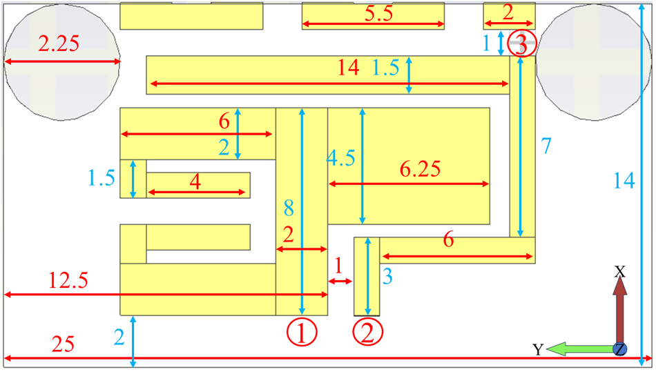
The antenna design is modified from the design presented in [Reference Ban, Liu, Chen, Li and Kang19] with more challenging space requirements. The unique goal is to retain most of the bandwidth in the LB and maintain the operation in the HB despite this space limitation. The design consists of a U-shaped feeding strip and two sections of shorting strips. The two sections of the shorting strips are connected using an inductor. The first part of this shorting strip is placed on the same PCB layer as the feeding strip, whereas its second part is bent in a meandered form inside the 3D-printed casing of the device. To enable more precise impedance tuning, the antenna aperture is tuned by an inductor (denoted by circle no 2), as shown in Fig. 6. The grounded meander line acts as an extension to the ground plane of the PCB, having the electrical length extended with the aperture tuning inductor [Reference Ali and Payandehjoo30]. Such method maintains design simplicity and avoids the need for inductance tuning using complex geometrical modifications due to space limitations.

Figure 6.

Meanderline structure with dimensions. 1) The feed location and 2) the aperture tuning component location.

Antenna simulations and optimization are performed using CST Microwave Studio Suite 2023, whereas optimization for the matching circuit is performed using Optenni Lab software [31]. The reconfigurable antenna system is designed on a cost-efficient, 1-mm thick FR4 substrate ( $\varepsilon_\mathrm{r}$ = 4.3 and metal thickness of 18 $\unicode{x03BC}$m). The PCB is housed in a 3D-printed case, with an area of 66 $\times$33 mm $^2$ and which lifts the PCB 10 mm from the bottom to allow placing the meander line below the PCB.

Antenna operation

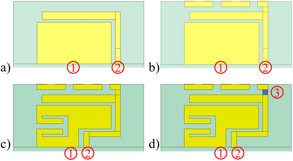
The initial design consists of a patch-like structure, feed position, and the grounded segment is denoted with 1 and 2, respectively, in Fig. 7. This provides the basis for the high-band operation of the structure, with the grounded segment being observed to significantly contribute to this behavior. The effect of the ground extension and aperture tuning from Fig. 7 is shown in Fig. 8.

Figure 7.

The different radiating structures, for which $|S_\mathrm{11}|$ results are shown in Figure 8: a) Grounded strip and simple patch, b) added meander line, c) modified patch, and d) additional aperture tuning inductor (2.2 nH, same as in the final structure of Figure 6). Here, (1) marks the feed port, (2) marks the grounding, and (3) marks the placement of the aperture tuning inductor.

Figure 8.

The effect of the different antenna parts on the input reflection coefficient $\left(|S_{11}|\right)$. The different design stages are visualized in Figure 7. The parts are not optimized for free-space operation; thus, the actual performance in this figure should only be regarded as a comparison between the accompanying results.

When adding the meander line structure, which extends below the ground plane of the PCB, as shown in Fig. 7(b), a new resonance appears at the low band. This modification also slightly boosts the high-band operation. In Fig. 7(c), the patch is modified to its final form by introducing a T-shaped cutout and moving the grounding point of the shorted strip. With this modification, the high-band performance is again slightly improved, and the low-band resonance shifts down in frequency.

To further tune the low-band operation, a discrete inductance (2.2 nH) is added between the grounded segment and the meander line. This shifts the low-band resonance toward the target range, with the amount of frequency shift defined by the additional inductance value. It can be observed that the higher the inductance value, the lower the frequency shifts. However, this comes at the cost of decreased total efficiency, and a proper evaluation of the trade-offs is required.

Antenna input matching

To further improve the antenna input impedance matching (to 50 $\Omega$) in the low band, lumped matching elements are used due to their compact size compared with that of the antenna. Besides that, these components also allow frequency tunability with a switching network.

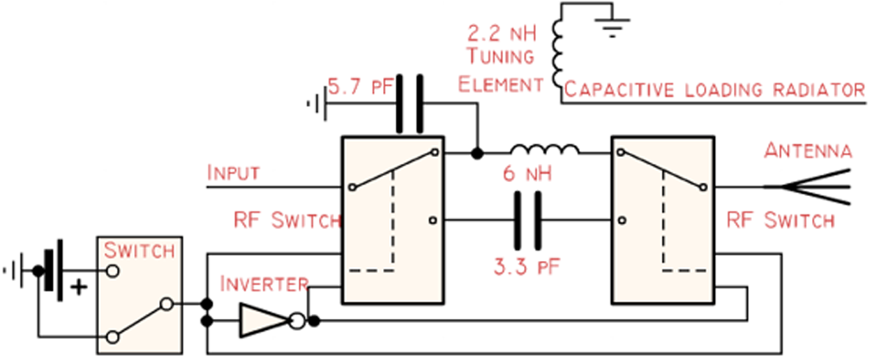
The radiating structure is shown in Fig. 9. It is designed in a switchable format to operate in two segments in the low band, using Configurations 1 (875–900 MHz) and 2 (898–934 MHz). In Fig. 10, the RF input is fed by an SMPM connector (Rosenberger) to a switched matching network. This network is switched between the two configurations using a simple combination of an inverter (Rohm) and a mechanical switch (Wurth) as a proof-of-concept. The matching networks are located between RF switches (Qorvo). The matching network for Configuration 1 consists of a parallel capacitor (Murata 5.7 pF) and a series inductor (Murata 6 nH). For Configuration 2, a simple series capacitor (Murata 3.3 pF) is used.

Figure 9.

Top view of the antenna element with dimensions annotated in mm. (1) Marks the feed location, (2) marks the grounding, and (3) the aperture tuning component location.

Figure 9 Long description

An antenna element with various dimensions annotated in millimeters. At the top left, a circle is labeled with a diameter of 2.25 millimeters. Adjacent to it, a horizontal line is marked with a length of 5.5 millimeters. Near the top right, another circle is labeled with a diameter of 2.25 millimeters. Below this, a horizontal line is marked with a length of 14 millimeters, followed by a smaller segment labeled 1.5 millimeters. The top right corner features a marked location labeled 3, indicating the aperture tuning component. Moving downwards, a vertical line is labeled with a length of 7 millimeters. Below this, a horizontal line is marked with a length of 6.25 millimeters. To the left, a vertical line is labeled with a length of 4.5 millimeters, followed by a horizontal line marked with a length of 4 millimeters. Below this, a vertical line is labeled with a length of 1.5 millimeters. The bottom left corner features a marked location labeled 1, indicating the feed location. Adjacent to it, a marked location labeled 2 indicates the grounding. A horizontal line at the bottom is marked with a length of 25 millimeters and a vertical line is labeled with a length of 12.5 millimeters. The diagram includes axes labeled X and Y at the bottom right corner, indicating orientation.

Figure 10.

Schematic of the matching- and control-circuit, with the used components annotated.

Figure 10 Long description

A switchable RF matching network is shown. It includes an RF switch connected to an input, leading to a parallel capacitor labeled 5.7 picofarads and a series inductor labeled 6 nanohenries. Another RF switch is connected to an antenna, with a series capacitor labeled 3.3 picofarads. A tuning element labeled 2.2 nanohenries is connected to a capacitive loading radiator. A mechanical switch and an inverter are connected in series, controlling the RF switches. The connections are clearly marked, with the RF switches positioned between the input and antenna, allowing for configuration changes in the network.

Measurement setup and body phantom

The optimized design was then fabricated, as shown in Fig. 11. $S$-parameter measurements were performed using an HP 8720ES vector network analyzer (VNA), whereas radiation patterns and efficiency were assessed using a SATIMO Starlab measurement system, as seen in Fig. 12. $S$-parameter measurements were performed on a homogeneous body phantom whose dimensions are 18 $\times$24 $\times$15 cm $^3$. The size of the phantom was then reduced to 10 $\times$20 $\times$8 cm $^3$ for the measurements of radiation pattern and efficiency due to the space and weight constraints on the antenna measurement platform. The simulated phantom shares the dielectric properties of the Basic phantom design of [32], and the phantom for measurements was made to match the same model using the recipe/part of the same recipe as the body model in [Reference Särestöniemi, Singh, Dessai, Heredia, Myllymäki and Myllylä33]. An RF cable and an SMPM-to-SMA adapter are used throughout the measurements.

Figure 11.

Close-up of the fabricated design, with the matching circuit and RF input.

Figure 12.

The reduced body phantom (10 $\times$20 $\times$8 cm $^3$) setup in the Satimo Starlab, for efficiency and gain measurements.

On-phantom measurements were performed using a 10 mm thick piece of Rohacell foam spacer, as seen in Fig. 13. The spacer is emulating the on-body adapter, which is included in the Bittium Faros^TM device [26]. Under the spacer, a piece of copper tape was used in on-body results as a reflector, as seen in Fig. 14, to reduce SAR, with a size roughly matching the size of the device [Reference Paracha, Rahim, Soh and Khalily20].

Figure 13.

On-body $S$-parameter measurements, with a 18 $\times$24 $\times$15 cm $^3$ body phantom.

Figure 14.

The Rohacell spacer and copper tape reflector next to the antenna.

Free space performance

Scattering parameters

Figure 15 presents the simulated and measured free space reflection coefficient for the antenna system. There is a slight shift upward in the measured resonant frequency in the low band and significant dampening in the matching compared to simulations. The high band displays an opposite behavior, with the measurement having a higher peak in the matching and the resonance in a slightly lower frequency, although the high band retains the required bandwidth.\RightSideStrip

Figure 15.

Simulated and measured reflection coefficient of the antenna in Free space. Here, Conf1 and Conf2 refer to the different matching network configurations.

Efficiency

Figure 16 shows the total efficiency of the antenna in free space. The efficiency peaks are around 0.9 GHz ( $-$4 dB), 0.93 GHz ( $-$3 dB), and 1.9 GHz ( $-$2 dB), which align well with the deepest resonances in the reflection coefficient of Fig. 15. A higher efficiency would be preferable, but ESAs have naturally low efficiency [Reference Nepa and Rogier7]. Although the measured reflection coefficient has a deeper notch at the high band compared to the simulation, the efficiency does not exhibit the same behavior. This is likely due to additional losses in actual components, which lower the peak efficiency of the prototype.

Figure 16.

Simulated and measured free space total efficiency of the antenna.

Radiation patterns

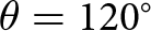
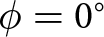
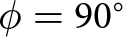
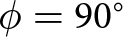
In Fig. 17, the simulated and measured gain is plotted for the free space case. The low band gain is slightly below 0 dB with deviation to as low as -10 dB, with a mostly omnidirectional pattern. The high band is similar with a deviation at $\phi=90^{\circ}$ and $\theta=120^{\circ}$ in Fig. 17(d).

Figure 17.

Simulated (dashed) and measured (solid) free-space radiation patterns at: (a) 920 MHz, $\phi$ = 0 $^{\circ}$ cut, (c) 920 MHz, $\phi$ = 90 $^{\circ}$ cut, (b) 1.9 GHz, $\phi$ = 0 $^{\circ}$ cut, and (d) 1.9 GHz, $\phi$ = 90 $^{\circ}$ cut. The orientation of the antenna can be seen in Figures 1 and 11. a) 920 MHz / $\phi=0^\circ$. b) 1.9 GHz / $\phi=0^\circ$. c) 920 MHz / $\phi=90^\circ$. d) 1.9 GHz / $\phi=90^\circ$.

Figure 17 Long description

A polar line plot labeled, theta. Text below reads, a, 920 megahertz slash phi equals 0 degrees. The angular scale is marked every 30 degrees from 0 degrees through 330 degrees. The radial tick labels are 10, 0, minus 10, minus 20 and minus 30. Two overlaid curves are shown, one solid and one dashed. The solid curve forms a rounded three lobe shape with a deeper inward dip near 90 degrees and another inward dip near 240 degrees. The dashed curve follows a similar shape with a deeper inward dip near 90 degrees. The image B showing a polar line plot labeled, theta. Text below reads, b, 1.9 gigahertz slash phi equals 0 degrees. The angular scale is marked every 30 degrees from 0 degrees through 330 degrees. The radial tick labels are 10, 0, minus 10, minus 20 and minus 30. Two overlaid curves are shown, one solid and one dashed. The solid curve is irregular with multiple lobes and a narrow inward notch near 120 degrees. The dashed curve is smoother and stays closer to a rounded shape, with a broader inward region near 120 degrees. The image C showing a polar line plot labeled, theta. Text below reads, c, 920 megahertz slash phi equals 90 degrees. The angular scale is marked every 30 degrees from 0 degrees through 330 degrees. The radial tick labels are 10, 0, minus 10, minus 20 and minus 30. Two overlaid curves are shown, one solid and one dashed. Both curves form a near circular shape, staying close to the 0 ring with small deviations. The image D showing a polar line plot labeled, theta. Text below reads, d, 1.9 gigahertz slash phi equals 90 degrees. The angular scale is marked every 30 degrees from 0 degrees through 330 degrees. The radial tick labels are 10, 0, minus 10, minus 20 and minus 30. Two overlaid curves are shown, one solid and one dashed. Both curves form a near circular shape close to the 0 ring, with a shallow inward dip around 180 degrees to 210 degrees. A legend below the plots labels the solid line as, Measured and the dashed line as, Simulated.

On-body performance

This subsection describes the on-body measurements and their results. The body phantom is described in Section III-A. with the general measurement setup.

Scattering parameters

The simulated and measured on-body reflection coefficients are shown in Fig. 18 for both switch configurations. The combined $-$6 dB bandwidth are from 875 MHz to 934 MHz in the low band, and from 1.7 GHz to 2.2 GHz in the high band The simulated low-band resonances are clearer (with significantly deeper dips) and a gap between the two configurations. In the high band, there is a more noticeable difference between the simulated and measured results relative to their performance in free space. Although both curves exhibit a dual-resonance response when operated in proximity to the body phantom, a larger gap between the two resonance peaks is observed in simulations.

Figure 18.

Comparison of simulated and measured on-body reflection coefficients. Bandwidth is defined according to the –6-dB matching criterion (indicated by the black dotted line).

The measured on-body bandwidth in the low band (875–934 MHz) is slightly wider than the simulated one (886–910 MHz) and covers the entire target frequency range. In the high band, the measured on-body results featured a bandwidth of 1714–2190 MHz, which almost satisfies the required bandwidth specifications. A larger discrepancy is seen in the high band due to the practical differences in the properties (relative permittivity and conductivity) of the phantoms across frequency. The properties of the phantom model used in simulations are extrapolated across the frequency of interest, whereas the properties of the fabricated phantom can be made close to the required values using the current manufacturing method in either the low or high band only. In this case, considering the more sensitive behavior of the antenna performance in the low band due to the larger distance needed to decouple them, the phantom has been fabricated based on the properties in this (low) band to evaluate the worst-case performance scenario of on-body coupling. Besides that, unlike in simulations, it is challenging to ensure that the fabricated phantom produces exact same homogeneous permittivity and conductivity in practice. Variation of these properties across the phantom’s width and length may occur and affect the accuracy of the measurement results. Despite these uncertainties, it is observed that the simulated and measured $|S_\mathrm{11}|$ in the high band exhibited similar bandwidths, with differences mainly observed in the depths of the resonances.

In Fig. 19(a), the low band curves show that the simulated results are overcoupled, while the measured results are undercoupled. On the other hand, in Fig. 19(b), the simulated high band results are undercoupled, whereas the measured results are almost critically coupled. When considering the high band results, the two simulated resonances of Fig. 18 are clearly visible as separate loops, whereas the measurements show a nascent dual resonance. Based on these observations, moving the impedance at the two resonances closer to the center of the Smith chart allows improvement of the overall matching level across the high band.

Figure 19.

Comparison of simulated and measured complex reflection coefficients. a) Low band: 0.6–1.2 GHz. b) High band: 1.5–2.5 GHz.

Figure 19 Long description

The first Smith chart represents the low band from 0.6 to 1.2 GHz, comparing simulated and measured complex reflection coefficients (S11). The chart is a normalized impedance Smith chart, typically referenced to 50 ohms. Simulated traces, labeled Sim Conf1 and Sim Conf2, form loops that differ from measured traces, labeled Meas Conf1 and Meas Conf2. Sim Conf1 forms a large loop near the outer regions, while Meas Conf1 shows a smaller loop closer to the center, indicating a mismatch in coupling. Sim Conf2 and Meas Conf2 also show differing loop shapes, with Meas Conf2 remaining closer to the center, suggesting better matching. The second Smith chart represents the high band from 1.5 to 2.5 GHz. Simulated trace Sim Conf2 forms multiple loops, while Meas Conf2 shows a nascent dual resonance with loops closer to the center, indicating improved matching compared to the simulated trace. The comparison highlights systematic deviations between simulated and measured traces, with measured traces generally showing better matching near the chart center, indicating improved resonance behavior.

Efficiency

The efficiency simulation uses the smaller body phantom due to the reasons mentioned in Section III-A. The total efficiency of an antenna refers to the power fed to it compared to the power radiated, accounting for all losses along the signal path. In this work, a total efficiency of at least $-$10 dB is desired throughout the operating frequency band. Results illustrated in Fig. 20 in both the low and high bands indicate that the total efficiencies correspond well to the reflection coefficient results, and the $-$10 dB target efficiency is achieved over the entire $-$6 dB bandwidth.

Figure 20.

Comparison of simulated and measured on-body total efficiency. The black line marks the –10 dB line used to determine the efficiency bandwidth.

Figure 20 Long description

The graphs display efficiency in decibels on the vertical axis, ranging from negative 35 to positive 5, against frequency in megahertz on the horizontal axis, divided into low and high bands. The low band ranges from 800 to 1000 megahertz, while the high band ranges from 1600 to 2200 megahertz. Four lines are plotted: Sim Conf1, Sim Conf2, Meas Conf1 and Meas Conf2. In the low band, Sim Conf1 peaks around 900 megahertz, reaching approximately negative 10 decibels, while Sim Conf2 follows a similar trend but slightly lower. Meas Conf1 and Meas Conf2 also peak near 900 megahertz, with Meas Conf1 reaching slightly above negative 10 decibels. In the high band, Sim Conf1 and Sim Conf2 maintain efficiency near negative 10 decibels across the frequency range, while Meas Conf1 and Meas Conf2 show more variation, with Meas Conf1 dropping below negative 20 decibels at certain points. The legend identifies each line with its corresponding configuration.

Compared to the free space efficiency in Fig. 16, only a drop of $-$2 dB is observed when the body phantom is introduced. This effect is contributed by the existence of the reflecting copper plate, and is also comparable to the study in [Reference Hall, Hao, Nechayev, Alomainy, Constantinou, Parini, Kamarudin, Salim, Hee, Dubrovka, Owadally, Song, Serra, Nepa, Gallo and Bozzetti8]. The difference between the low band efficiencies is a result of the lower frequency that affects the electrical size and radiation characteristics of the antenna.

Radiation patterns

The current ESA system is intended to be used on the body to collect ECG-based health information and channel it to a base station. Therefore, in this application, the antenna radiation patterns need to be designed appropriately, with the main beam pointing away from the user. At the same time, the existence of the ground plane will ensure that the performance of the antenna is not easily influenced by the coupling to the body. Moreover, high back radiation can increase SAR levels, and this should be avoided.

Prior to the on-body radiation pattern measurement, the size of the body phantom was reduced (from 18 $\times$24 $\times$15 cm $^3$ to 10 $\times$20 $\times$8 cm $^3$) to comply with the mechanical rotation of the StarLab measurement system. Nonetheless, it is expected that this change will have minimal effects in evaluating the true performance of the antenna on the body, as the distance from the edges of the antenna to the edges of the body model is at least 0.1 $\lambda$. In Fig. 21, the gain patterns for the design are shown, for both the low band (920 MHz) and the high band (1.9 GHz), on two different axes. The gain toward the body is significantly increased in measurements in the low band, as seen in Fig. 21(a) and (b). In other aspects, the measured gain is similar to the simulated gain. Gain simulations were also performed using the smaller body phantom model.

Figure 21.

Simulated (dashed) and measured (solid) on-body radiation patterns at: (a) 920 MHz, $\phi$ = 0 $^{\circ}$ cut, (c) 920 MHz, $\phi$ = 90 $^{\circ}$ cut, (b) 1.9 GHz, $\phi$ = 0 $^{\circ}$ cut, and (d) 1.9 GHz, $\phi$ = 90 $^{\circ}$ cut. The orientation of the antenna can be seen in Figures 1 and 11. a) 920 MHz / 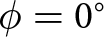$\phi=0^\circ$. b) 1.9 GHz / 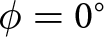$\phi=0^\circ$. c) 920 MHz / 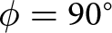$\phi=90^\circ$. d) 1.9 GHz / 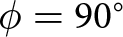$\phi=90^\circ$.

Figure 21 Long description

The polar plot A is labeled, 920 megahertz slash phi equals 0 degrees. Angular labels run from 0 degrees at the top through 30, 60, 90, 120, 150, 180, 210, 240, 270, 300 and 330 degrees. The radial scale is labeled 10, 0, minus 10, minus 20 and minus 30. Two curves are shown, one solid and one dashed. The solid curve is near 0 to minus 10 around 0 degrees, then moves inward toward about minus 20 to minus 30 between about 210 degrees and 270 degrees, with a small inward notch near about 240 degrees. The dashed curve follows a similar shape but is more inward between about 210 degrees and 270 degrees. The polar plot B is labeled, 1.9 gigahertz slash phi equals 0 degrees. Angular labels run from 0 degrees at the top through 30, 60, 90, 120, 150, 180, 210, 240, 270, 300 and 330 degrees. The radial scale is labeled 10, 0, minus 10, minus 20 and minus 30. Two curves are shown, one solid and one dashed. Both curves are near 0 to 10 around 0 degrees. Both move inward toward about minus 20 to minus 30 around 180 degrees, forming a narrow inward region centered near 180 degrees. The solid curve shows side bulges around about 240 degrees and 300 degrees compared with the dashed curve. The polar plot C is labeled, 920 megahertz slash phi equals 90 degrees. Angular labels run from 0 degrees at the top through 30, 60, 90, 120, 150, 180, 210, 240, 270, 300 and 330 degrees. The radial scale is labeled 10, 0, minus 10, minus 20 and minus 30. Two curves are shown, one solid and one dashed. The solid curve stays close to 0 to minus 10 from about 300 degrees through 60 degrees, then moves inward to around minus 10 to minus 20 near 180 degrees, with a rounded inward dip centered near 180 degrees. The dashed curve is inside the solid curve over most angles, with the largest separation near 180 degrees. The polar plot D is labeled, 1.9 gigahertz slash phi equals 90 degrees. Angular labels run from 0 degrees at the top through 30, 60, 90, 120, 150, 180, 210, 240, 270, 300 and 330 degrees. The radial scale is labeled 10, 0, minus 10, minus 20 and minus 30. Two curves are shown, one solid and one dashed. Both curves are near 0 to 10 around 0 degrees and remain near 0 around 90 degrees and 270 degrees. Near 180 degrees, both curves form multiple narrow inward notches, reaching toward about minus 20 to minus 30, with the solid curve showing deeper and more jagged notches than the dashed curve. A legend below the plots shows solid line labeled, Measured and dashed line labeled, Simulated.

Specific absorption rate

The SAR is a measure of power absorption in body tissue/phantom, and its limit is 1.6 W/kg averaged over a 1-g mass of tissue according to the Federal Communications Commission (FCC) standards in the United States [3]. This regulation is chosen as it is one of the strictest. In comparison, the IEEE limit is 2 W/kg averaged over 10 g of tissue, which is relatively easier to obtain.

In this work, the SAR for the band-switchable ESA system is simulated in CST using a homogeneous body phantom. An accepted power of 23 dBm was used to roughly match a possible use case power. A 10-mm gap is chosen to emulate the spacing between the antenna and human body in an actual use case, which includes the ECG electrode and an adapter for the device. The effect of the additional metal layer is evaluated in terms of reflection coefficients in Fig. 22. In the low band, a stronger resonance peak is seen for Configuration 1, without any obvious changes in Configuration 2. On the other hand, in the high band, a similar increase in resonance strength is noticed for the resonance peaks, resulting in a slight degradation of the reflection coefficient in the center of the whole high band. Despite this, the measured $|S_\mathrm{11}|$ of the prototype with the phantom in the high band indicated satisfactory performance while producing SAR values within the accepted regulatory level.

Figure 22.

Simulated reflection coefficient with (Sim) and without (NC) the SAR reduction layer. Both of the results employ a 10 mm gap between the model and the phantom.

Figure 22 Long description

Reflection Coefficient [dB]. Frequency [MHz]. Two side by side line graphs labeled Low band and High band. Low band graph. The y-axis is labeled Reflection Coefficient [dB], ranging from 0 to minus 20 with ticks at 0, minus 2, minus 4, minus 6, minus 8, minus 10, minus 12, minus 14, minus 16, minus 18 and minus 20. The x-axis is labeled Frequency [MHz], ranging from 800 to 1000 with ticks at 800, 850, 900, 950 and 1000. A horizontal dotted reference line is drawn at minus 6. Four curves are shown with a legend: NC Conf1 as a dotted line, NC Conf2 as a solid line, Sim Conf1 as a dotted line and Sim Conf2 as a solid line. All four curves form a single sharp notch centered near 900 MHz. The dotted NC Conf1 curve drops to about minus 18 near 900 MHz and returns to about minus 1 to minus 2 near 800 and near 1000. The solid NC Conf2 curve drops to about minus 12 near 900 MHz and returns to about minus 1 to minus 2 near 800 and near 1000. The dotted Sim Conf1 curve drops to about minus 16 near 900 MHz and returns to about minus 1 to minus 2 near 800 and near 1000. The solid Sim Conf2 curve drops to about minus 10 near 900 MHz and returns to about minus 1 to minus 2 near 800 and near 1000. High band graph. The y-axis is labeled Reflection Coefficient [dB], ranging from 0 to minus 20 with ticks at 0, minus 2, minus 4, minus 6, minus 8, minus 10, minus 12, minus 14, minus 16, minus 18 and minus 20. The x-axis is labeled Frequency [MHz], ranging from 1600 to 2300 with ticks at 1600, 1800, 2000 and 2200. A horizontal dotted reference line is drawn at minus 6. Four curves are shown with the same legend labels and line styles as the low band graph. The dotted NC Conf1 curve stays near minus 1 to minus 2 across the range with a shallow dip around 1800 to 1900. The solid NC Conf2 curve has a notch near about 1800 reaching about minus 10, then rises toward about minus 4 to minus 5 around 2000, then drops again to a deeper notch near about 2200 reaching about minus 15 and rises again toward about minus 6 to minus 7 near 2300. The dotted Sim Conf1 curve stays near minus 1 to minus 2 with a shallow dip around 1800 to 1900. The solid Sim Conf2 curve follows a similar shape to the solid NC Conf2 curve, with a notch near about 1800 reaching about minus 8, then a higher section around 2000 near about minus 4 to minus 5, then a deeper notch near about 2200 reaching about minus 12 to minus 13 and then rising toward about minus 6 to minus 7 near 2300.

The SAR results are shown in Table 1, indicating satisfactory compliance with the safety levels. These SAR levels can be further reduced by modifications of the transmit power duty cycle [Reference Zradziński, Karpowicz and Gryz35]. Besides that, future research could include more advanced and compact metamaterial-based solutions such as artificial magnetic conductor (AMC) reflectors [Reference Atrash, Abdalla and Elhennawy36–Reference il Kwak, Sim, Kwon and Yoon38] to reduce SAR levels by limiting backward radiation. However, such solutions come at the cost of a larger area requirement for their implementation, as they are typically designed in the form of an array of unit cells at their operating frequency. Considering the need for such a reflector in the low band in this case, a significantly compact AMC reflector is needed to ensure full compliance with the current operation of the health monitoring device in practice. This is certainly a challenging aspect that can be pursued in the next stage of the research. It should be noted that SAR measurements were not possible at the time of the investigation. However, considering the reasonably large safety margins from the SAR limits, it can be expected that the measured values would also fall well within the acceptable limits [Reference Soh, Vandenbosch, Wee, van den Bosch, Martinez-Vazquez and Schreurs39].

Table 1.

Simulated SAR results with an accepted power of 23 dBm and when averaging over a 1-g mass of tissue

Table 1 Long description

SAR results are reported in watts per kilogram for two columns, Configuration 1 and Configuration 2, across two rows, Low band resonance and High band 1.9 gigahertz. In the Low band resonance row, Configuration 1 is 0.433 at 0.910 gigahertz and Configuration 2 is 0.379 at 0.923 gigahertz. In the High band 1.9 gigahertz row, Configuration 1 is 0.461 and Configuration 2 is 0.246. Within Configuration 1, the high band value is higher than the low band value. Within Configuration 2, the high band value is lower than the low band value.

Comparison with the state-of-the-art

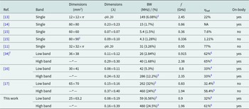
In the literature, there are only a few similar works on ESA design for on-body operation, which also include measurements. Nonetheless, several of the most relevant works are compared in Table 2. In [Reference Ruaro, Thaysen and Jakobsen13], an ESA working at 2.4 GHz is introduced for hearing aid applications. The research does not focus on bandwidth enhancement, but rather on improving radiation efficiency. In [Reference Orefice, Pirinoli and Dassano14], an ESA designed to operate in the sub-1 GHz band is proposed. The size is significantly larger, and the investigation is focused on the wearable aspect and radiation patterns. On the other hand, in [Reference Virushabadoss, Quaye and Henderson15], two designs for operation below 400 MHz are proposed. Both designs are remarkably compact compared to their frequency. However, this significantly affects the achieved bandwidth. Neither of the designs is meant for on-body use, but as a study into ESAs. Next, in [Reference Tang, Lin and Ziolkowski11], a Yagi-based antenna with polarization reconfigurability is introduced. This design utilizes the vertical space in the enclosing ESA sphere with a stacked design. In [Reference Sambandam, Kanagasabai, Mohammed, Thirunavukkarasu, Shanmuganathan, Ramadoss and Palaniswamy34], a small wearable antenna is introduced. The achieved footprint is small, and the targeted frequency bands are narrow, but sufficient. This design also achieves good efficiency. In [Reference Garcia, Andújar, Pijoan and Anguera17], a reconfigurable antenna system is proposed, operating from 698–960 MHz and from 1710–2170 MHz. This is achieved using a seven-state switchable matching network, enabling wide bandwidths in both frequency bands of interest with decent efficiency. However, as this method relies heavily on the ground plane, it may not be practical to achieve the targets in this work, besides not being intended for on-body use. Perhaps the most relevant comparison for this work is from [Reference Hajj, Person and Wiart16], in which a rectangular-spiral dual-band antenna operating in similar frequencies is proposed. Moreover, the effect of the proximity to the body is studied. A major difference between that work and the proposed antenna lies in the antenna-to-ground plane size ratio, which is more restricted in this work.

Table 2.

Comparison with other relevant work

Table 2 Long description

Rows compare antenna references by band, physical dimensions in millimeters squared, electrical size in wavelengths, bandwidth in megahertz and percent, frequency in gigahertz, radiation efficiency, and whether results are on body. Single band entries include reference 13 at 2.45 gigahertz with 149 megahertz bandwidth and 22 percent radiation efficiency on body, reference 14 at 0.86 gigahertz with 15 megahertz bandwidth and radiation efficiency not given on body, and reference 11 at 0.95 gigahertz with 31 megahertz bandwidth and 77 percent radiation efficiency not on body. Reference 15 lists two single band designs not on body, one at 0.36 gigahertz with 5.4 megahertz bandwidth and 7.6 percent radiation efficiency, and one at 0.336 gigahertz with 4.3 megahertz bandwidth and 1.21 percent radiation efficiency. Dual band entries include reference 34 with a low band at 0.915 gigahertz, 26 megahertz bandwidth and 62 percent radiation efficiency on body, and a high band at 2.38 gigahertz, 40 megahertz bandwidth and 65 percent radiation efficiency on body. Reference 16 lists a low band at 0.8 gigahertz, 42 megahertz bandwidth and 33 percent radiation efficiency on body, and a high band at 2.35 gigahertz, 286 megahertz bandwidth and 33 percent radiation efficiency on body. Reference 17 lists a low band at 0.83 gigahertz, 262 megahertz bandwidth and 32.4 percent radiation efficiency not on body, and a high band at 1.94 gigahertz, 460 megahertz bandwidth and 58.4 percent radiation efficiency not on body. For this work, the low band uses dimensions 25 by 63.2 millimeters with electrical size 0.08 by 0.19 wavelengths, and the high band uses the same physical dimensions with electrical size 0.16 by 0.39 wavelengths.

¹ With a 150×140mm² ground plane.

² –6dB bandwidth, compared with –10dB bandwidth.

³ The high band cannot be considered as electrically small.

⁴ With 12mm to the phantom.

⁵ Averaged total efficiency.

⁶ Total efficiency.

⁷ Two bands at higher frequencies not reported here.