1 Introduction
Magnetospheric physics results from a complex interaction between the solar wind with its imbedded magnetic field – the interplanetary magnetic field (IMF) – the magnetosphere itself and the ionosphere. During the past several years we have been developing a new simulation approach in which we combine a global magnetohydrodynamic (MHD) simulation of this interaction with an implicit particle-in-cell (PIC) simulation. With this approach we can model magnetospheric dynamics driven by observed solar wind parameters. We have used this to investigate magnetic reconnection.
Geomagnetic activity in the solar wind, magnetosphere and ionosphere occurs when solar wind with a southward directed IMF component interacts with Earth’s magnetic field at the dayside magnetopause through the process of magnetic reconnection. Following reconnection magnetic flux is convected from the sunward side of the magnetosphere to the magnetic tail where a second reconnection occurs which returns the flux to the dayside. In this process mass, momentum and energy are transferred from the solar wind to the magnetosphere system. In our studies we modelled both the dayside reconnection process (Lapenta et al. Reference Lapenta, Berchem, Zhou, Walker, El-Alaoui, Goldstein, Paterson, Giles, Pollock and Russell2017) and the tail reconnection (Ashour-Abdalla et al. Reference Ashour-Abdalla, Lapenta, Walker, El-Alaoui, Liang, Berchem and Goldstein2016; Lapenta et al. Reference Lapenta, Ashour-Abdalla, Walker and El-Alaoui2016; Walker et al. Reference Walker, Lapenta, Liang, Berchem, Ashour-Abdalla and Goldstein2018; Zhou et al. Reference Zhou, El-Alaoui, Lapenta, Berchem, Richard, Schriver and Walker2018).
The actual magnetic reconnection process involves two scales. The larger region is the ion diffusion region. In this region the ions are unmagnetized. It scales as the ion inertial length given by
 $d_{i}=c/\unicode[STIX]{x1D714}_{pi}$
with
 $c$
the speed of light and
 $\unicode[STIX]{x1D714}_{pi}$
the ion plasma frequency (
 $\unicode[STIX]{x1D714}_{pi}=\sqrt{ne^{2}/\unicode[STIX]{x1D700}_{0}m_{i}}$
where
 $n$
is the plasma density,
 $e$
is the electron charge,
 $\unicode[STIX]{x1D700}_{0}$
is the vacuum dielectric constant and
 $m_{i}$
is the mass of the ion) and can be several Earth radii (
 $\text{R}_{\text{E}}$
) in extent. The actual reconnection process occurs in the electron diffusion region (EDR). It is much smaller and scales as the electron skin depth given by
 $d_{e}=c/\unicode[STIX]{x1D714}_{pe}$
where
 $\unicode[STIX]{x1D714}_{pe}$
is the electron plasma frequency (
 $\unicode[STIX]{x1D714}_{pe}=\sqrt{ne^{2}/\unicode[STIX]{x1D700}_{0}m_{e}}$
where
 $m_{e}$
is the mass of the electron).
At the dayside magnetopause, we investigated the crescent shaped electron velocity space distributions observed in the EDR by the spacecraft of the Magnetospheric Multiscale Scale (MMS) mission (Burch et al. Reference Burch2016). The appearance of these crescent shaped distribution functions in the perpendicular direction was key to determining the location of the EDR. In this study we carried out a pair of high-resolution simulations which captured sub-ion skin-depth scales (Lapenta et al. Reference Lapenta, Berchem, Zhou, Walker, El-Alaoui, Goldstein, Paterson, Giles, Pollock and Russell2017). The results showed that the crescent shaped distribution functions observed by MMS are caused by electrons on meandering orbits without requiring any other processes and that these distribution functions are to be found whenever there are thin current sheets. We also found in both theory and observations that these crescent shaped distributions show up in the ion distribution functions in the larger region where ions are on meandering orbits.
Our initial studies were not on the sunward side of the magnetosphere but in the magnetotail. There we used our new approach to investigate additional ways of locating the EDR during a magnetospheric substorm by considering other diagnostics. In the following
 $\boldsymbol{E}$
is the electric field vector,
 $\boldsymbol{B}$
is the magnetic field and
 $\boldsymbol{v}_{\boldsymbol{e}}$
is the electron velocity. These indicators of the EDR are: (i) slippage
 $|\unicode[STIX]{x1D6FF}\boldsymbol{v}_{\boldsymbol{e}_{\bot }}|\equiv |\boldsymbol{v}_{\boldsymbol{e}\bot }-\boldsymbol{E}\times B/B^{2}|$
where
 $_{\bot }$
indicates the components perpendicular to the magnetic field. (ii) The non-ideal terms in Ohm’s law. For electrons the non-ideal terms are given by
 $|\boldsymbol{E}+\boldsymbol{v}_{e}\times \boldsymbol{B}|=|(1/ne)\unicode[STIX]{x1D735}\boldsymbol{\cdot }\unicode[STIX]{x1D64B}_{\mathbf{e}}+((-1/e)(D/Dt)(m_{e}\boldsymbol{v}_{\boldsymbol{e}}))|$
where
 $\unicode[STIX]{x1D64B}_{\mathbf{e}}$
is the electron pressure tensor,
 $m_{e}$
is the electron mass and
 $e$
is the electron charge (Goldman, Newman & Lapenta Reference Goldman, Newman and Lapenta2015). The non-ideal terms in Ohm’s law can be evaluated by using the left-hand side of this equation and calculating
 $|\boldsymbol{E}_{\text{non}\text{-}\text{ideal}}|=|\boldsymbol{E}+\boldsymbol{v}_{\boldsymbol{e}}\times \boldsymbol{B}|$
. (iii) The work done by the electromagnetic fields on particles during the reconnection process. Here we have calculated the work done in the electron frame
 $\boldsymbol{J}\boldsymbol{\cdot }\boldsymbol{E}^{\prime }=\boldsymbol{J}\boldsymbol{\cdot }(\boldsymbol{E}+\boldsymbol{v}_{\boldsymbol{e}}\times \boldsymbol{B})$
where
 $\boldsymbol{J}$
is the current density. Zenitani et al. (Reference Zenitani, Hesse, Klimas, Black and Kuznetsova2011) have investigated the work done and derived a new expression
 $\boldsymbol{J}\boldsymbol{\cdot }\boldsymbol{E}^{\prime }=\boldsymbol{J}\boldsymbol{\cdot }(\boldsymbol{E}+\boldsymbol{v}_{\mathbf{e}}\times \boldsymbol{B})-\unicode[STIX]{x1D70C}\boldsymbol{v}_{\boldsymbol{e}}\boldsymbol{\cdot }\boldsymbol{E}$
where
 $\unicode[STIX]{x1D70C}$
is the charge density. The extra term results from the frame change which can lead to an extra current. (iv) Non-gyrotropic electron distribution functions. Three methods have been suggested (Scudder & Daughton Reference Scudder and Daughton2008; Aunai, Hesse & Kuznetsova Reference Aunai, Hesse and Kuznetsova2013; Swisdak Reference Swisdak2016). We used the approach suggested by Scudder & Daughton (Reference Scudder and Daughton2008), but the other methods led to similar results in the calculations discussed in this paper. The agyrotropy (non-gyrotropy) is calculated by using
 $A_{e}=2((\unicode[STIX]{x1D706}_{\bot 1}-\unicode[STIX]{x1D706}_{\bot 2})/(\unicode[STIX]{x1D706}_{\bot 1}+\unicode[STIX]{x1D706}_{\bot 2}))$
where
 $\unicode[STIX]{x1D706}_{\bot 1}$
and
 $\unicode[STIX]{x1D706}_{\bot 2}$
are the eigenvalues of the electron pressure tensor (
 $\unicode[STIX]{x1D64B}_{\mathbf{e}}$
) in the plane normal to
 $\boldsymbol{B}$
.
We found that all of diagnostics gave false positive values but that by using three of the diagnostics (slippage, Ohm’s law and agyrotropy) together along with requiring the magnetic field north–south component to be zero we could identify the EDR (Ashour-Abdalla et al.
Reference Ashour-Abdalla, Lapenta, Walker, El-Alaoui, Liang, Berchem and Goldstein2016; Walker et al.
Reference Walker, Lapenta, Liang, Berchem, Ashour-Abdalla and Goldstein2018). We had expected that
 $\boldsymbol{J}\boldsymbol{\cdot }\boldsymbol{E}^{^{\prime }}$
would be positive as electromagnetic energy was converted into particle energy. The big surprise was that
 $\boldsymbol{J}\boldsymbol{\cdot }\boldsymbol{E}^{^{\prime }}$
in the reconnection region alternated between positive and negative. This was especially evident in the
 $Y$
-direction and was associated with strong electron flows in the negative
 $Y$
(dawnward) direction. The results are consistent with those expected for the lower hybrid drift instability coupled with a shear type instability such as the Kelvin–Helmholtz instability (Walker et al.
Reference Walker, Lapenta, Liang, Berchem, Ashour-Abdalla and Goldstein2018).
In this paper, we present a detailed discussion of the approach to the combined MHD and PIC simulation. This is presented in §§ 2–4. In § 2, we discuss the overall approach to linking the codes. In § 3 we consider the initialization of the PIC simulation while in § 4 we discuss the boundary conditions. Next we demonstrate this approach by examining results from simulation studies of reconnection in the magnetotail. In particular, we will show results from two simulations of the same reconnection event. The first simulation is the one discussed above (Ashour-Abdalla et al. Reference Ashour-Abdalla, Lapenta, Walker, El-Alaoui, Liang, Berchem and Goldstein2016; Lapenta et al. Reference Lapenta, Ashour-Abdalla, Walker and El-Alaoui2016 and Walker et al. Reference Walker, Lapenta, Liang, Berchem, Ashour-Abdalla and Goldstein2018). The second is from a simulation of this event carried out with twice the number of grid points in each direction. Comparison of the two runs in § 5 shows that the overall results presented in Ashour-Abdalla et al. (Reference Ashour-Abdalla, Lapenta, Walker, El-Alaoui, Liang, Berchem and Goldstein2016) and Walker et al. (Reference Walker, Lapenta, Liang, Berchem, Ashour-Abdalla and Goldstein2018) are robust. We discuss the simulation results in § 6.
2 Approach for linking PIC and MHD codes
The fluid (MHD) and kinetic formulations are not incompatible. Fluid models can be rigorously derived from kinetic models by using the moment approach. However, the reverse is not trivial because information on the phase space distribution is lost by taking moments. Additionally, if the fluid model is single fluid MHD, some of the information distinguishing the electron fluid from the ion fluid is also lost.
We have created a kinetic model that spins off of an evolving fluid state. As soon as the kinetic calculation is started, the kinetic state begins to evolve differently than the fluid state. We do not attempt to modify the fluid evolution to take into account this kinetic evolution. That is, the coupling between fluid and kinetic states is one way. The idea is that we follow the evolution for a relatively short time so that the kinetic effects do not have time to modify the macroscopic evolution to an important degree.
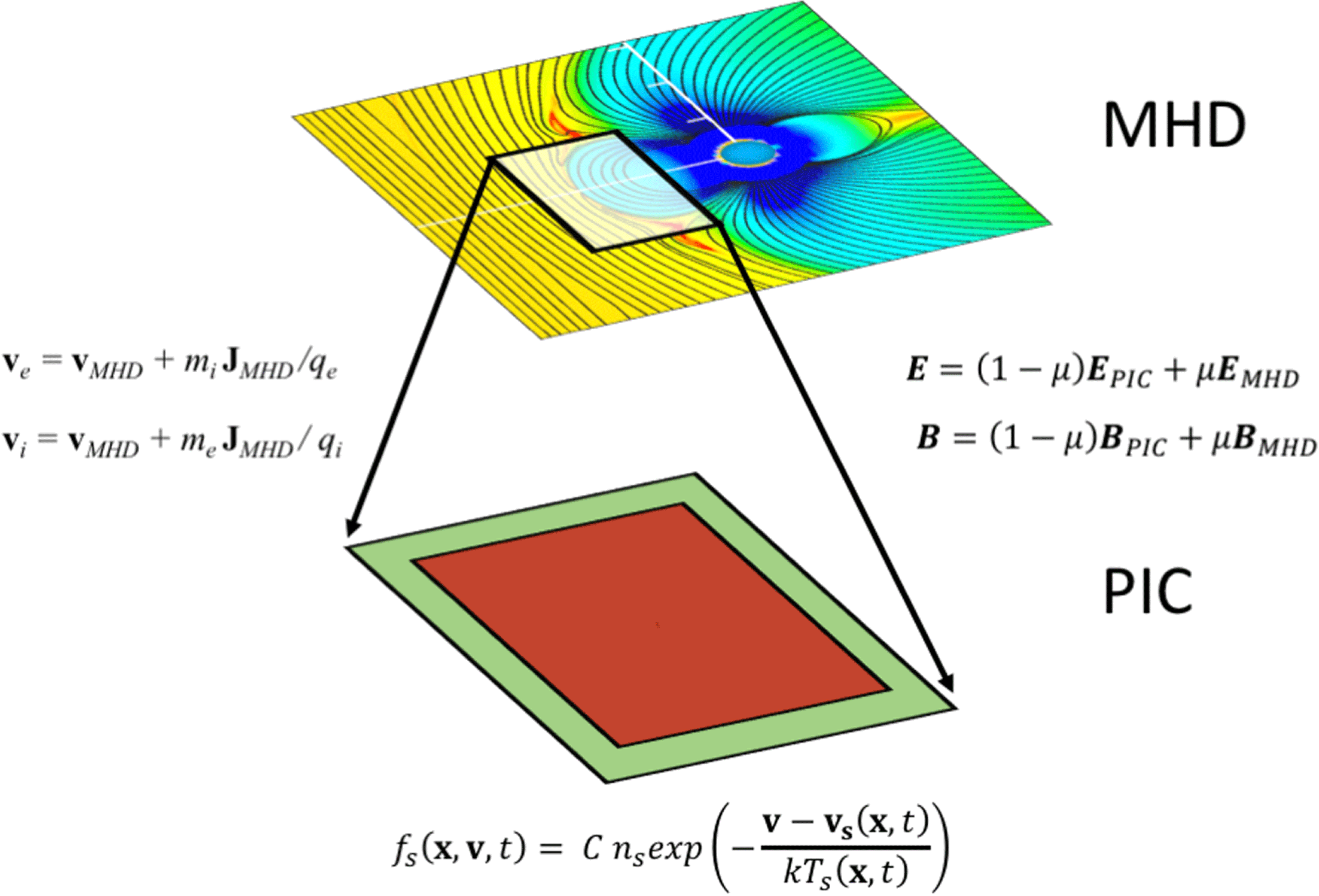
Even one way coupling is a challenge requiring a number of numerical techniques to arrive at a stable and accurate kinetic model. Figure 1 summarizes the idea. A fluid model covers the whole system while the kinetic code covers only a smaller sub-domain. The kinetic code needs information from the fluid run to start and to assign the boundary conditions.
We first run a fluid simulation. In the present case, we use the UCLA global MHD magnetospheric model (Raeder, Walker & Ashour-Abdalla Reference Raeder, Walker and Ashour-Abdalla1995; Raeder, Berchem & Ashour-Abdalla Reference Raeder, Berchem and Ashour-Abdalla1998; El-Alaoui Reference El-Alaoui2001; El-Alaoui et al.
Reference El-Alaoui, Ashour-Abdalla, Walker, Peroomian, Richard, Angelopoulos and Runov2009). At a given time during the evolution of the calculation, chosen by the user for its potential interest, we spawn a PIC simulation of a smaller subdomain of the fluid state. For the PIC model, we use iPic3D (Markidis, Lapenta & Rizwan-Uddin Reference Markidis, Lapenta and Rizwan-Uddin2010) for its implicit nature that allows us to use relatively larger scales than an explicit PIC code, reducing the gap between the scales described by the fluid and kinetic models. The iPic3D method is based on the implicit moment method (Brackbill & Forslund Reference Brackbill and Forslund1982; Lapenta Reference Lapenta2012). The iPic3D code solves the full set of particle equations for electrons and ions. In the examples in this paper, we use the classical limit but the code includes a relativistic mover. The code uses the full set of Maxwell’s equations, discretized by using a second-order formulation based on the electric field. The field equations are solved for the electric field (
 $\boldsymbol{E}$
) while the magnetic field (
 $\boldsymbol{B}$
) is computed afterwards from Faraday’s law. The code uses the implicit moment method to discretize the coupled set of particles and fields equations. The resulting discretization has better energy conservation properties than explicit formulations and allows the user to relax the stability requirements on the time step and grid resolution.
To solve the field equations, a grid is introduced where the electric field is defined on the vertices of the discretization while the magnetic field is defined in the centres. A notable advantage of the second-order approach is that no boundary conditions are needed for the magnetic field. The magnetic field at the cell centres is computed from the electric field on the vertices of the cell: no magnetic field resides on the boundary. We have, however, to supply boundary conditions for the electric field. In the next section we describe how the PIC run is initialized and how the boundary conditions are set.
Illustration of the coupling of a fluid and a kinetic domain. The information needed to initialize the PIC domain is obtained from the MHD domain. The boundary conditions are set in a boundary layer (in green) where we can either impose open conditions (perfectly matched layer) or MHD-driven values. The equations listed transfer information from MHD to PIC.

3 Initialization of the PIC domain
A kinetic state is not fully defined by a fluid state. The electric and magnetic fields are given but the particle information is provided only via the first moments: density, velocity and temperature. This information cannot determine a kinetic distribution function. An arbitrary assumption is needed. Kinetic theory suggests using a Boltzmann distribution because the H theorem states that overall the entropy tends to increase and at equilibrium it reaches a maximum (Cercignami Reference Cercignami2012) where the Boltzmann distribution
 $$\begin{eqnarray}f_{s}(\boldsymbol{x},\boldsymbol{v},t)=Cn_{s}\exp \left(-\frac{\boldsymbol{v}-\boldsymbol{v}_{\boldsymbol{s}}(\boldsymbol{x},t)}{kT_{s}(\boldsymbol{x},t)}\right)\end{eqnarray}$$
for each species
 $s$
(electrons or ions) applies. However, space is not an equilibrium and spacecraft often encounter distributions far from the Boltzmann case. For example, power laws (kappa distributions) are pervasive in the Universe and could be used in place of the Boltzmann distribution. Since there is no way of knowing a priori which distribution to use, practice guides what distribution is best. Once the distribution is selected, the system will evolve and produce distributions far from the initial thermal equilibrium.
Whatever distribution is used, electrons and ions will not usually have the same parameters. For two fluid models these moments are known but even single fluid MHD determines completely the lowest-order moments. The local density
 $n_{s}$
is equal for both species (electrons and ions) to ensure quasi-neutrality. The local speed of both species is determined by taking together the local MHD speed (
 $\boldsymbol{v}_{\text{MHD}}$
) and current density (
 $\boldsymbol{J}_{\text{MHD}}$
):
 $$\begin{eqnarray}\left.\begin{array}{@{}c@{}}\boldsymbol{v}_{e}=\boldsymbol{v}_{\text{MHD}}+m_{i}\,\boldsymbol{J}_{\text{MHD}}/q_{e}\\ \boldsymbol{v}_{i}=\boldsymbol{v}_{\text{MHD}}+m_{e}\,\boldsymbol{J}_{\text{MHD}}/q_{i},\end{array}\right\}\end{eqnarray}$$
where the mass and charge of the ions and electrons are used. The temperature is not defined completely. Our MHD model uses a single scalar temperature. This requires us to assume a data-inspired temperature ratio between the species. For instance, ions are observed to be on average approximately 5 times hotter than the electrons in the magnetotail. (See Artemyev et al. (Reference Artemyev, Baumjohann, Petrukovich, Nakamura, Dandouras and Fazakerley2011) for a discussion of the temperature ratio in the magnetotail plasma sheet.) Therefore, the ion temperature is assumed equal to the MHD temperature but the electron temperature is
 $1/5$
of that. This approach can be improved if the fluid models have a pressure tensor, so different temperatures can be assigned in different directions. Even off-diagonal terms of the pressure tensor can be accommodated within Boltzmann distributions based on the Chapman–Enskog expansion (Garcia & Alder Reference Garcia and Alder1998).
The initial state generated with this approach is not an exact solution of a Vlasov equation. The spatially varying electric and magnetic fields are self-consistent only with the first moments (
 $n$
,
 $\boldsymbol{v}$
and
 $T$
) of the distribution function but are not self-consistent with respect to the full distribution function. The Boltzmann distribution is a solution only if there are no spatial variations. The presence of spatial variations, even though self-consistent with the first moments, will lead to imbalances in the higher-order moments: anisotropic components of the pressure tensor, heat flux and higher. For this reason, after initialization, the kinetic simulation undergoes relaxation. The implicit moment method is advantageous in this situation because it tends to damp high frequency and short wavelength waves (Brackbill & Forslund Reference Brackbill and Forslund1982). This damping facilitates the elimination of noise and the establishment of a proper kinetic state after a short transient following the initial set-up.
4 Boundary conditions of the PIC domain
The most critical aspect of coupling fluid and kinetic models is the strategy for handling the boundary conditions. We rely here on the progress made in the study of the multi-level multi-domain method (Innocenti et al. Reference Innocenti, Lapenta, Markidis, Beck and Vapirev2013). We use two types of boundary conditions, semi-open or driven by MHD.
The semi-open boundary conditions are the same as those used in other applications of iPic3D (Lapenta et al. Reference Lapenta, Markidis, Goldman and Newman2015). The approach extends to the implicit particle-in-cell method the perfectly matched layer (Berenger Reference Berenger1994). In a layer next to the boundary, a damping term is added to Maxwell’s equations to absorb outgoing waves:
 $$\begin{eqnarray}\frac{\unicode[STIX]{x2202}\boldsymbol{E}}{\unicode[STIX]{x2202}t}=\unicode[STIX]{x1D735}\times \boldsymbol{B}-\unicode[STIX]{x1D706}\boldsymbol{E},\end{eqnarray}$$
where
 $\unicode[STIX]{x1D706}$
is a damping rate increasing monotonically from zero at the inner boundary of the damping region to its maximum value at the external boundary of the PIC domain (Berenger Reference Berenger1994). The particles in the boundary layer are replaced at every time step with a new population based on the reference state provided by the MHD run.
The MHD-driven boundary conditions are identical to the semi-open boundary conditions for the particles but not for the fields. The fields are imposed from the MHD state:
 $$\begin{eqnarray}\left.\begin{array}{@{}c@{}}\boldsymbol{E}=(1-\unicode[STIX]{x1D707})\boldsymbol{E}_{\text{PIC}}+\unicode[STIX]{x1D707}\boldsymbol{E}_{\text{MHD}}\\ \boldsymbol{B}=(1-\unicode[STIX]{x1D707})\boldsymbol{B}_{\text{PIC}}+\unicode[STIX]{x1D707}\boldsymbol{B}_{\text{MHD}},\end{array}\right\}\end{eqnarray}$$
where
 $\unicode[STIX]{x1D707}=\unicode[STIX]{x1D706}/\max (\unicode[STIX]{x1D706})$
smoothly transitions the field from the internal value computed by the PIC method to the value imposed by MHD.
Figure 1 shows the boundary layer as a green area. The thickness of the boundary layer can be varied. In the results reported so far the layer has a thickness of 3 cells in the magnetotail runs and 100 in the magnetopause runs.
5 Application to reconnection in the magnetotail
5.1 Simulation set-up
Our first application of this approach was to simulate reconnection in the magnetotail during a magnetospheric substorm observed on February 15, 2008 (Zhou et al.
Reference Zhou, Ashour-Abdalla, Deng, Schriver, El-Alaoui and Pang2009; Ashour-Abdalla et al.
Reference Ashour-Abdalla, El-Alaoui, Goldstein, Zhou, Schriver, Richard, Walker, Kivelson and Hwang2011). This interval was first modelled by using the UCLA single fluid global MHD simulation (Raeder et al.
Reference Raeder, Walker and Ashour-Abdalla1995, Reference Raeder, Berchem and Ashour-Abdalla1998; El-Alaoui Reference El-Alaoui2001; El-Alaoui et al.
Reference El-Alaoui, Ashour-Abdalla, Walker, Peroomian, Richard, Angelopoulos and Runov2009). This code solves the single fluid particle moment equations along with Maxwell’s equations. In our approach, the input to the MHD simulation is given by setting the solar wind and interplanetary magnetic field (IMF) parameters upstream from Earth’s bow shock based on observations in the solar wind. For this substorm, the solar wind observations were from the Cluster satellites located in the solar wind near the bow shock. We placed a state selected from the MHD output and then placed a large PIC simulation domain in the magnetotail. In geocentric solar magnetospheric (GSM) coordinates (Russell Reference Russell1971; Hapgood Reference Hapgood1992) it extended over
 $-45\text{R}_{\text{E}}<X<-15\text{R}_{\text{E}}$
,
 $-3\text{R}_{\text{E}}<Y<9\text{R}_{\text{E}}$
,
 $-9\text{R}_{\text{E}}<Z<3\text{R}_{\text{E}}$
(
 $275d_{i}\times 110d_{i}\times 110d_{i}$
where
 $d_{i}$
is the ion inertial length). We have run the same simulation with two grids. The PIC simulation box was loaded by using results from the MHD simulation starting at 0348:00UT (Ashour-Abdalla et al.
Reference Ashour-Abdalla, Lapenta, Walker, El-Alaoui, Liang, Berchem and Goldstein2016; Lapenta et al.
Reference Lapenta, Ashour-Abdalla, Walker and El-Alaoui2016) and run for 154 s. Magnetotail reconnection had already started in the MHD simulation at this time and continued in the MHD model throughout the duration of the PIC run (Ashour-Abdalla et al.
Reference Ashour-Abdalla, Lapenta, Walker, El-Alaoui, Liang, Berchem and Goldstein2016). In our initial studies we investigated how the reconnection evolved from this time. In our earlier studies (Ashour-Abdalla et al.
Reference Ashour-Abdalla, Lapenta, Walker, El-Alaoui, Liang, Berchem and Goldstein2016; Lapenta et al.
Reference Lapenta, Ashour-Abdalla, Walker and El-Alaoui2016; Walker et al.
Reference Walker, Lapenta, Liang, Berchem, Ashour-Abdalla and Goldstein2018), we presented results using a box with
 $400\times 160\times 160$
grid points. The time step was
 $\unicode[STIX]{x1D714}_{ce}\unicode[STIX]{x0394}t=0.03$
where
 $\unicode[STIX]{x1D714}_{ce}$
is the electron cyclotron frequency and the cell size in each dimension was
 $0.25d_{e}$
assuming a reference density of
 $n_{0}=0.25~\text{cm}^{-3}$
. There were
 $1.28\times 10^{9}$
particles of each species in the simulation. For the second simulation we used
 $800\times 320\times 320$
grid points and a total of
 $1.024\times 10^{10}$
particles. The time step was half that in the lower-resolution run. The mass ratio was 256 in both simulations with realistic ions and more massive electrons. As discussed below the main conclusions were the same. This strengthens our conviction that the approach is solid.
5.2 Tail reconnection results
Magnetotail reconnection began in the mid-tail at
 $X\sim -30R_{E}$
and
 $Y\sim 2\text{R}_{\text{E}}$
at
 ${\sim}03:48:38~\text{UT}$
. Ashour-Abdalla et al. (Reference Ashour-Abdalla, Lapenta, Walker, El-Alaoui, Liang, Berchem and Goldstein2016) reported that the reconnection site moved quickly across the tail in the
 $Y$
-direction reaching the dusk boundary in approximately 2 minutes (see the movie in Walker et al.
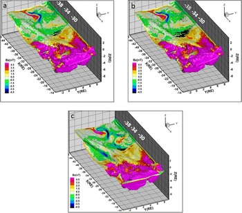
Reference Walker, Lapenta, Liang, Berchem, Ashour-Abdalla and Goldstein2018). In figure 2 we present a snapshot 10 s after reconnection began (24 000 time steps into the lower resolution simulation) where we have plotted the
 $B_{z}$
-component of the magnetic field on the
 $B_{x}=0$
surface. The original calculation at this time is in (a,b) and the higher-resolution simulation is on the bottom (c). In (a), we have placed iso-surfaces of agyrotropy greater than 0.3 using the definition of Scudder & Daughton (Reference Scudder and Daughton2008) while in (b) we show iso-surfaces of agyroropy greater than 0.2. Note we have not interpolated the results to the current sheet. The only places where the agyrotropy is larger than these values is in the current sheet. In (b) there are two regions with values of agyrotropy greater than 0.2. One is at
 $X\sim -31\text{R}_{\text{E}}$
and one is at
 $X\sim 36\text{R}_{\text{E}}$
.
 $B_{z}$
changes sign at both locations. The values of agyrotropy in the current sheet are larger nearer Earth. The agyrotropy is always less than 0.3 at the more distant site. We will see later the earthward component of velocity also changes there. In (c) only the iso-surfaces for agyrotropy greater than 0.2 are shown. Again both
 $B_{z}$
and the agyrotropy are consistent with two locations of reconnection. The two simulations give results for
 $B_{z}$
that are very similar but the agreement is not exact. In both calculations the regions with positive (northward) field (warm colours) and negative (southward) field (cool colours) occur in the same region but the values differ slightly. For instance the value of positive
 $B_{Z}$
earthward of the earthward most reconnection site are slightly larger in the higher-resolution simulation. That
 $B_{z}$
changes sign and the changes are associated with enhanced agyrotropy suggest that these are multiple sites of reconnection aligned in roughly in the
 $X$
direction in both simulations.
The surface
 $B_{x}=0$
becomes very irregular in the morning earthward most quadrant in both cases (magenta coloured region in both panels). This is caused by turbulent flows in that region (Ashour-Abdalla et al.
Reference Ashour-Abdalla, Lapenta, Walker, El-Alaoui, Liang, Berchem and Goldstein2016). We have limited our studies of reconnection so far to the better organized region on the dusk side of the tail.
The
 $B_{Z}$
-component of the magnetic field on the surface defined by
 $B_{X}=0$
. The results for
 $B_{Z}$
have been interpolated by using inverse distance interpolation. The results from the lower-resolution simulation are on the top (a,b) and those from the higher-resolution simulation are on the bottom (c). The black bars are iso-surfaces of agyrotropy greater than 0.3 in (a) and greater than 0.2 in (b,c). There are two places where
 $B_{Z}$
changes sign and the agyrotropy is enhanced.

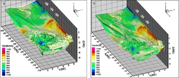
We have displayed the
 $V_{x}$
-component of the electron velocity in figure 3. Here (a) is from the lower-resolution simulation and (b) is from the higher-resolution run. As is the case in figure 2, the results are similar but not identical. The flows reverse direction where
 $B_{z}$
does. This is consistent with the finding that reconnection is occurring in those two regions. Duskward of
 $Y\sim 6\text{R}_{\text{E}}$
the flow tailward of the earthward most field direction change is earthward in both simulations (between
 $X\sim -32\text{R}_{\text{E}}$
and
 ${\sim}-34\text{R}_{\text{E}}$
). These earthward flows result from reconnection occurring at the more tailward site. In Walker et al. (Reference Walker, Lapenta, Liang, Berchem, Ashour-Abdalla and Goldstein2018) we found similar flows from multiple reconnection sites later in the simulation.
The
 $V_{x}$
component of the electron velocity in the surface defined by
 $B_{x}=0$
. (a) Contains the results from the lower-resolution simulation and (b) contains the results from the higher-resolution simulation.

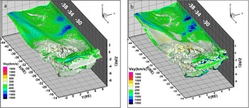
In figure 4 we present the electron flows in the
 $Y$
direction from the two simulations. In the region with enhanced agyrotropy the
 $V_{y}$
flows are strongly in the minus
 $Y$
direction. The strongest
 $V_{y}$
flows are in the region of enhanced agyrotropy where the magnetic field changes sign. They exceed
 $1400~\text{km}~\text{s}^{-1}$
in the lower-resolution simulation and
 $1800~\text{km}~\text{s}^{-1}$
in the higher-resolution simulation. In Walker et al. (Reference Walker, Lapenta, Liang, Berchem, Ashour-Abdalla and Goldstein2018), using the lower-resolution simulation, we showed that these diamagnetic flows were one of the main reasons that the slippage was large in regions outside of the EDR. Only in the EDR was slippage dominated by the
 $V_{x}$
component (Walker et al.
Reference Walker, Lapenta, Liang, Berchem, Ashour-Abdalla and Goldstein2018, table 1). These results were confirmed by the higher-resolution simulation.
We repeated the analyses in figures 2–4 with agyrotropy values of 0.05, 0.1 and 0.15 in addition to 0.2. For the three values there were regions of enhanced agyrotropy in the lobes. Only values greater than
 ${\sim}0.2$
were confined to the putative reconnection regions in the current sheet. In general we found evidence for the EDR where agyrotropy was greater than 0.2 suggesting that for this event the agyrotropy must exceed
 ${\sim}0.2$
for it to be an indicator of the EDR. In Walker et al. (Reference Walker, Lapenta, Liang, Berchem, Ashour-Abdalla and Goldstein2018) we found that in general the agyrotropy at the magnetotail reconnection site decreases with distance from the Earth. This is also the case for the higher-resolution simulation.
The
 $V_{y}$
component of the electron velocity on the
 $B_{x}=0$
surface. (a) Contains the results from the lower-resolution simulation and (b) contains the results from the higher-resolution simulation.

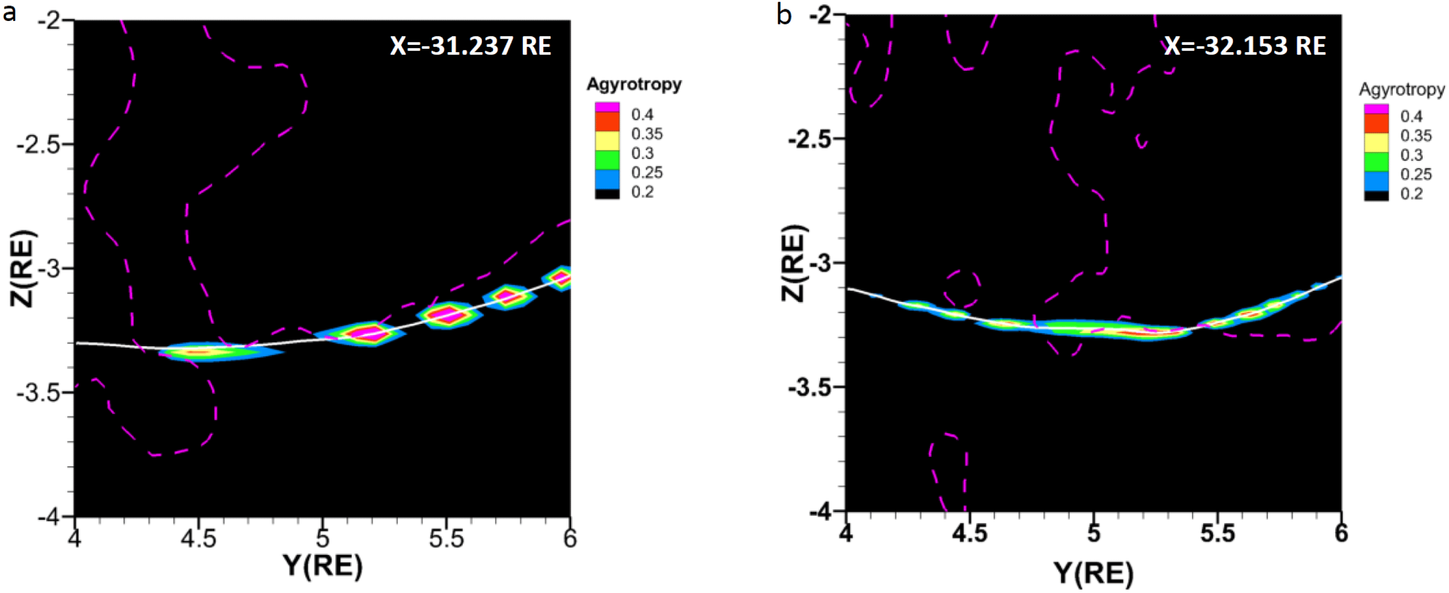
The agyrotropy,
 $B_{z}=0$
contours and
 $B_{x}=0$
contours in
 $YZ$
planes from the lower-resolution simulation (a) and the higher-resolution simulation (b). Note that the planes are separated by approximately
 $0.9\text{R}_{\text{E}}$
. This is because the location where the agyrotropy is largest and
 $B_{z}=0$
are not co-located in the two simulations.

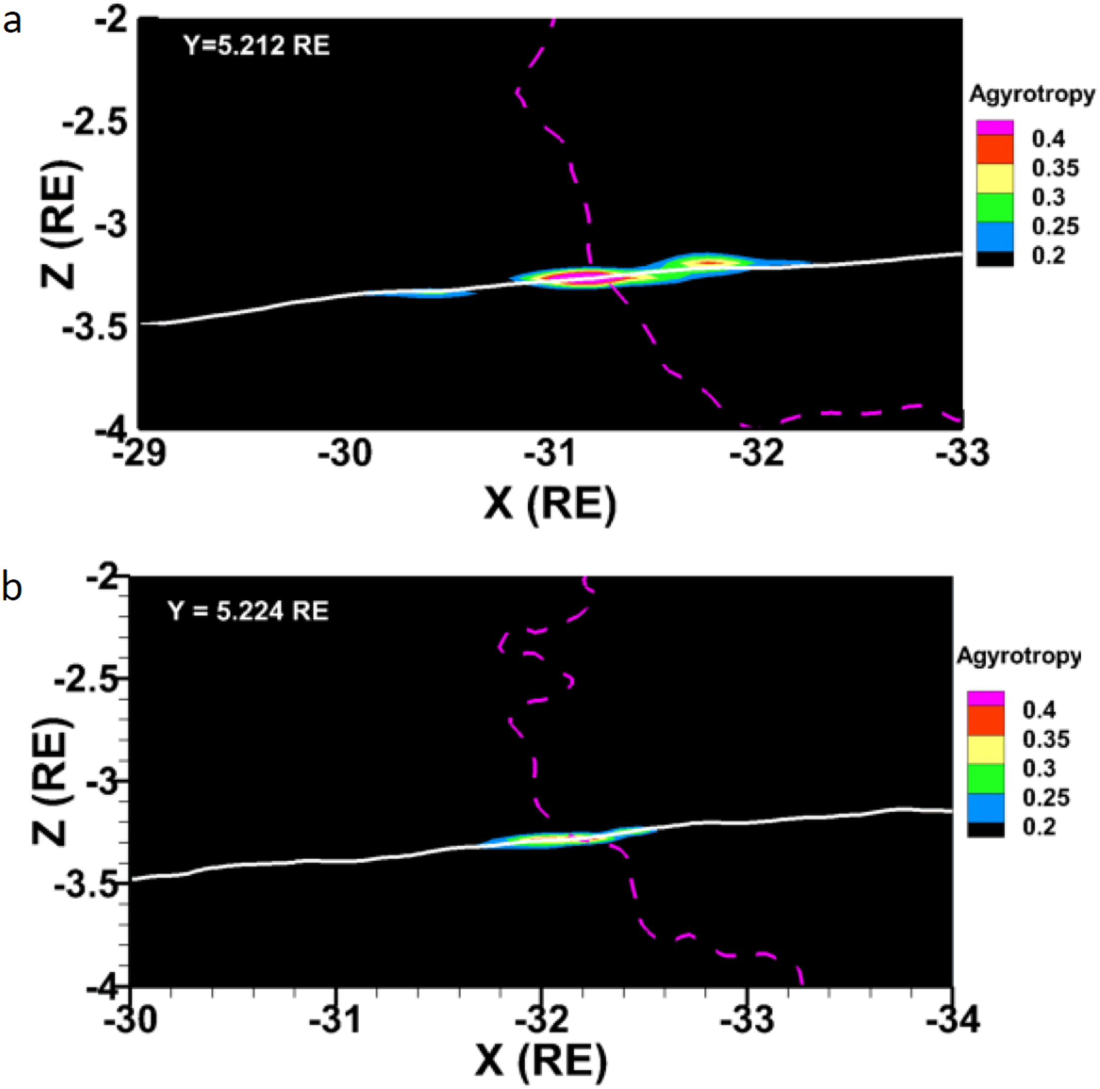
The agyrotropy,
 $B_{z}=0$
contour (dashed magenta line) and the
 $B_{x}=0$
contour (solid white line) from the lower-resolution simulation (a) and the higher-resolution simulation (b) in constant
 $Y$
planes. Note that the
 $Y$
planes are slightly displaced from each other. The slices are confined to the grid in this plot. We have not interpolated the values. Also note that the
 $X$
-axis in (b) has been shifted by
 $1\text{R}_{\text{E}}$
tailward with respect to (a).

One of the most unexpected findings in our earlier studies was that the reconnection was structured in the
 $Y$
-direction. All of the diagnostics we tested (slippage, the non-ideal terms in Ohm’s law, agyrotropy and the work
 $(\boldsymbol{J}\boldsymbol{\cdot }\boldsymbol{E}^{\prime }=\boldsymbol{J}\boldsymbol{\cdot }(\boldsymbol{E}+\boldsymbol{v}_{\boldsymbol{e}}\times \boldsymbol{B}))$
) had structure in the azimuthal direction. In figures 5 and 6 we present blow ups of the agyrotropy from figure 2. In this analysis we closely examined the results to find the location in the current sheet where
 $B_{z}$
changes sign. In figure 5 we have plotted the agyrotropy in two constant
 $X$
planes. Both simulations have structure in the agyrotropy in the
 $Y$
-direction. The region with the largest agyrotropy in both is at
 $Y\sim 5.2\text{R}_{\text{E}}$
. That also is where
 $B_{z}=0$
in both plots but they are separated by about
 $0.9\text{R}_{\text{E}}$
in
 $X$
. In figure 6 we show that the location of reconnection is shifted tailward in the higher-resolution simulation. In figure 6(a) the location of reconnection is at about
 $X=-31.2\text{R}_{\text{E}}$
while in (b) it is at approximately
 $X=-32.1\text{R}_{\text{E}}$
. In addition in both panels of figure 5 the regions of enhanced agyrotropy do not always correspond to
 $B_{z}=0$
.
5.3 Discussion of the tail results
The two simulations are very similar overall (figures 2–4) but as we have pointed out they differ in detail. Why then are they different? Although both simulations are based on the same MHD simulation and start from the same initial time and state they must be populated independently since the cells are different. Thus as soon as they start they begin to evolve differently. For this reason we do not expect the results to be identical. Recall the lower-resolution simulation results in this report were taken at 24 000 time steps into the simulation. The higher-resolution results are from time step 48 000. In any simulation, small initial differences will accumulate in time. The important consideration is whether the physics is the same.
Overall the values of the parameters plotted in figures 2–4 are similar as are the locations in the simulations. However, they are not identical. There are multiple reconnection sites in the tail characterized by a change in the sign of
 $B_{z}$
, earthward electron flows, enhanced agyrotropy, increased slippage in the region dominated by the
 $V_{x}$
term and an increase in the non-ideal terms in Ohm’s law. The results for slippage and Ohm’s law are like those in figures 6–9 and table 1 of Walker et al. (Reference Walker, Lapenta, Liang, Berchem, Ashour-Abdalla and Goldstein2018). At this time both simulations show evidence for two reconnection sites. One in the near tail (between
 $X=-31\text{R}_{\text{E}}$
and
 $-32.5\text{R}_{\text{E}}$
) and one deeper in the tail. The biggest differences in the two simulations are in the exact locations of reconnection (figures 5 and 6). The near-Earth reconnection site in the higher-resolution case at
 $Y=\,\sim \,5.2\text{R}_{\text{E}}$
is about
 $0.9\text{R}_{\text{E}}$
tailward of that at lower resolution. Throughout the interval simulated, multiple locations of reconnection were common. In Walker et al. (Reference Walker, Lapenta, Liang, Berchem, Ashour-Abdalla and Goldstein2018) we identified three possible reconnection locations aligned later in the simulation (step 34 000 in the lower-resolution simulation). It is not too surprising that the two runs gave different locations in the near tail since the runs evolve slightly differently during the simulation because of the different loading. The initial configuration used in the simulation came from a time step in the MHD simulation in which there was a long region with a very thin current sheet (
 ${<}0.4\text{R}_{\text{E}}$
thick (Ashour-Abdalla et al.
Reference Ashour-Abdalla, Lapenta, Walker, El-Alaoui and Liang2015)). In such a thin current sheet the small initial differences in the simulation parameters can lead to differences in the reconnection location. The figures in this paper are single snapshots of the dynamic tail configuration. The movie in Walker et al. (Reference Walker, Lapenta, Liang, Berchem, Ashour-Abdalla and Goldstein2018) shows that the number of reconnection sites changes throughout the 154 s in the simulation. As explained above the two simulations are showing slightly different states of the tail.
Both simulations show considerable structure in the
 $Y$
-direction as well as in the
 $X$
-direction. It is interesting to note that the regions of enhanced agyrotropy in figures 5 and 6 are not always locations where
 $B_{Z}=0$
. In Walker et al. (Reference Walker, Lapenta, Liang, Berchem, Ashour-Abdalla and Goldstein2018) we argued that the structure may be related to secondary instabilities found in the reconnection process and not only related to reconnection. In Walker et al. (Reference Walker, Lapenta, Liang, Berchem, Ashour-Abdalla and Goldstein2018) we discuss examples of this in PIC simulations based on a Harris sheet.
The implicit code enables us to run large simulations in realistic magnetospheric configurations. It does this by allowing us to use larger grid spacing and time steps than in explicit simulations which must resolve the Debye length everywhere. The question then is can we still resolve the electron diffusion region? A number of studies have addressed this question (e.g. Ricci et al.
Reference Ricci, Brackbill, Daughton and Lapenta2004; Lapenta et al.
Reference Lapenta, Markidis, Goldman and Newman2010). The implicit code resolves the Debye length and the electron skin depth in the EDR because the density decreases. As noted in § 5.1 the cell size in the lower-resolution run is
 $0.25d_{e}$
so we can resolve the EDR. In the plasma sheet the plasma beta
 $\unicode[STIX]{x1D6FD}\gg 1$
. In a high
 $\unicode[STIX]{x1D6FD}$
plasma the frozen-in condition is broken by the non-gyrotropic terms in the pressure tensor (Kuznetsova, Hesse & Winski Reference Kuznetsova, Hesse and Winski2001; Pritchett Reference Pritchett2001; Ricci, Lapenta & Brackbill Reference Ricci, Lapenta and Brackbill2002). Ricci et al. (Reference Ricci, Brackbill, Daughton and Lapenta2004) have used both implicit and explicit codes to study reconnection in a Harris sheet. They find that even though the implicit code does not fully capture all of the high frequency modes, the reconnection rates are the same. The frozen in flux condition is broken by non-gyrotropic terms in the pressure tensor as expected.
6 Conclusions
We have used results from our modelling of magnetic reconnection in the magnetotail to demonstrate the technique of embedding implicit particle-in-cell simulations in global MHD simulations. It is a powerful approach to investigate kinetic processes in the magnetosphere. This approach allows us to extend the MHD models and to investigate additional physical processes under realistic magnetospheric conditions over large regions of the magnetosphere.
Acknowledgements
The work at UCLA was supported by a NASA Heliospheric Grand Challenges grant 80NSSC17K0014 and NSF grant AGS-1450864. In addition the work is supported by the Onderzoekfonds KU Leuven (Research Fund KU Leuven), by the Interuniversity Attraction Poles Programme of the Belgian Science Policy Office (IAP P7/08 CHARM) and by the DEEP-ER and DEEP-EST project of the European Commission. The simulations were conducted on NASA NCCS and HECC supercomputers, and on the VSC Flemish Supercomputing Centre and on the facilities provided by PRACE research infrastructure Tier-0 grants. This research used resources of the National Energy Research Scientific Computing Center, a DOE Office of the Science User Facility supported by the Office of Science of the U.S. Department of Energy under Contract No. DE-AC02-05CH11231. The simulation results used in this paper are available from the Virtual Magnetospheric Observatory http://vmo.igpp.ucla.edu/.