1. Introduction
The structural nature of turbulent boundary layers has been the subject of many investigations. Over the last half a century, a large number of studies have shown that turbulent boundary layers are populated by a hierarchy of recurrent structures, commonly referred to as ‘coherent structures’. These include: low- and high-speed streaks (Kline et al. Reference Kline, Reynolds, Schraub and Runstadler1967; Offen & Kline Reference Offen and Kline1975), ejection and sweeps (Wallace, Eckelmann & Brodkey Reference Wallace, Eckelmann and Brodkey1972), streamwise vortices (Blackwelder & Eckelmann Reference Blackwelder and Eckelmann1979), hairpin vortices (Theodersen Reference Theodersen1952; Offen & Kline Reference Offen and Kline1974; Head & Bandyopadhyay Reference Head and Bandyopadhyay1981), large-scale three-dimensional bulges (Falco Reference Falco1977), packets of hairpin vortices (Head & Bandyopadhyay Reference Head and Bandyopadhyay1981; Zhou et al. Reference Zhou, Adrian, Balachandar and Kendall1999; Adrian, Meinhart & Tomkins Reference Adrian, Meinhart and Tomkins2000), very-large-scale motions (Kim & Adrian Reference Kim and Adrian1999) and superstructures (Hutchins & Marusic Reference Hutchins and Marusic2007). Significant effort has been put into investigating coherent motions to understand their scaling laws, generation/interaction mechanisms, and their role in the production and dissipation of turbulence (Smits, McKeon & Marusic Reference Smits, McKeon and Marusic2011; Herpin et al. Reference Herpin, Stanislas, Foucaut and Coudert2013). Further efforts have also been made in an attempt to model these structural features, with models based on hairpin or packet-like structures gaining broad interest (summarised recently by Adrian Reference Adrian2007 and Adrian & Marusic Reference Adrian and Marusic2012).
Experimental evidence of hairpins in turbulent boundary layers was observed by Offen & Kline (Reference Offen and Kline1974, Reference Offen and Kline1975), followed by Head & Bandyopadhyay (Reference Head and Bandyopadhyay1981) who formed a structural link between the near-wall and the outer-flow behaviour. It was concluded that these structures are a major constituent of the turbulent boundary layer, and their work described several geometric properties of hairpin-like structures, including their characteristic angle to the wall and aspect ratio. One notable observation of Head & Bandyopadhyay (Reference Head and Bandyopadhyay1981) was that hairpin vortices could organise into larger coherent groups. This important notion lead to a large range of studies investigating this phenomenon. For example, studies by Acarlar & Smith (Reference Acarlar and Smith1987a ,Reference Acarlar and Smith b ) showed that the insertion of a single hairpin vortex into a laminar boundary layer could generate a series of small hairpins, which then travel as a group (packet) with a common convection velocity. The notion of coherent packets of hairpins evolving from independent hairpin structures was also demonstrated in simulations by Zhou et al. (Reference Zhou, Adrian, Balachandar and Kendall1999).
Alternative explanations to the hairpin-packet paradigm include the notion of ‘superbursts’ (Na, Hanratty & Liu Reference Na, Hanratty and Liu2001), where large-Reynolds-stress-producing events are observed as regions of relatively low-momentum fluid. del Álamo et al. (Reference del Álamo, Jiménez, Zandonade and Moser2004) showed similar structures, but attributed these log-region phenomena to passive wakes formed downstream of vortex clusters. An extension of this work by del Álamo et al. (Reference del Álamo, Jiménez, Zandonade and Moser2006) showed that the length and width of these clustered vortices are proportional to their wall-normal height, and further developments are reviewed by Jiménez (Reference Jiménez2012). More recently, simulations by Schlatter et al. (Reference Schlatter, Li, Örlü, Hussain and Henningson2014) at moderate Reynolds numbers have also highlighted that hairpin-like structures which extend to the wall are not observed instantaneously, in contrast to the findings of Wu & Moin (Reference Wu and Moin2009) (see also discussion in Marusic (Reference Marusic2009) regarding this on-going debate). For an extensive overview of structures and coherent motions in wall turbulence, readers are directed towards recent summaries by Marusic & Adrian (Reference Marusic, Adrian, Davidson, Yukio and Sreenivasan2012) and Herpin et al. (Reference Herpin, Stanislas, Foucaut and Coudert2013), and more recent developments concerning large- and very-large-scale motions are discussed in Baltzer, Adrian & Wu (Reference Baltzer, Adrian and Wu2013) and Lee et al. (Reference Lee, Lee, Choi and Sung2014).
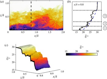
Meinhart & Adrian (Reference Meinhart and Adrian1995) reported the existence of large and irregularly shaped regions of uniform streamwise momentum (hereafter referred to as a uniform momentum zone, or UMZ). They reported that these UMZs were commonly observed encapsulating the logarithmic region. Meanwhile, the wake region of the boundary layer seemed to be populated with complicated and time-varying patterns of zones of uniform streamwise momentum. This zonal structural arrangement is best described with reference to figure 1(a), where a randomly selected streamwise–wall-normal velocity field is shown from a particle image velocimetry (PIV) measurement to be described shortly. Qualitatively, the zonal-like structure in the streamwise velocity is evident by visual inspection, where three regions of relatively uniform streamwise momentum are observed for the selected velocity field at the highlighted streamwise location (
 $x/{\it\delta}=0.8$
, where
 ${\it\delta}$
corresponds to the boundary layer thickness). Closer inspection of the instantaneous mean velocity profile at
 $x/{\it\delta}=0.8$
(figure 1
b) shows that, unlike the average velocity profile (shown by the blue dashed line), the instantaneous counterpart consists of sudden step-like jumps in streamwise momentum as one passes from one UMZ to another (see also figure 1
c which shows a three-dimensional surface of the streamwise velocity (
 $\widetilde{U}$
) in the range
 $0.8<x/{\it\delta}<1$
).
(a) Colour contours of streamwise velocity (
 $\widetilde{U}^{+}$
) at
 $Re_{{\it\tau}}\approx 8000$
from a single PIV frame. (b) Comparison between an instantaneous (——) and mean (– –) velocity profile. Horizontal dotted lines correspond to possible separations of zones of constant streamwise momentum; for this example, three possible UMZs are observed, labelled
 $\unicode[STIX]{x2460}$
,
 $\unicode[STIX]{x2461}$
and
 $\unicode[STIX]{x2462}$
. (c) Three-dimensional streamwise velocity contours for
 $0.85<x/{\it\delta}<1$
and
 $0<z/{\it\delta}<1$
. The black contour line shows the instantaneous streamwise velocity profile in
 $z$
at
 $x/{\it\delta}=0.8$
(as also plotted in b).

A more extensive study on UMZs was detailed in Adrian et al. (Reference Adrian, Meinhart and Tomkins2000), where it was shown that UMZs are prevalent and persistent for large streamwise lengths (of the order of
 ${\it\delta}$
). They hypothesised that these features were linked to the existence of packet-like hairpin structures, and coupled their results with numerical work from Zhou et al. (Reference Zhou, Adrian, Balachandar and Kendall1999) to construct a conceptual model. This model has been shown to explain several quantitative results seen in both experimental and numerical work to date. Tomkins & Adrian (Reference Tomkins and Adrian2003) performed a complementary set of experiments in the same turbulent boundary layer as Adrian et al. (Reference Adrian, Meinhart and Tomkins2000) but in a streamwise–spanwise plane from the buffer layer to the top of the logarithmic region. Here, the dominant motions were shown to be large-scale, low-momentum zones elongated in the streamwise direction, which are bordered by organised vortices. Similar experimental observations were also made by Ganapathisubramani, Longmire & Marusic (Reference Ganapathisubramani, Longmire and Marusic2003) and Hambleton, Hutchins & Marusic (Reference Hambleton, Hutchins and Marusic2006). Recent large-scale direct numerical simulations (DNS) by Lee & Sung (Reference Lee and Sung2011) showed groups of hairpin vortices which are coherently arranged in the streamwise direction. They observed that these structures combined to create significantly elongated low- and high-momentum regions (large-scale motions) of the order of
 $3{\it\delta}$
–
 $4{\it\delta}$
.
The presence of structural features is not easily observable with single-point measurements. However, a co-spectral analysis between the wall-normal velocity and spanwise vorticity by Priyadarshana et al. (Reference Priyadarshana, Klewicki, Treat and Foss2007) (later extended by Morrill-Winter & Klewicki Reference Morrill-Winter and Klewicki2013) from well-resolved hot-wire measurements showed both high- and low-wavenumber peaks. They hypothesised that the high-wavenumber peak is associated with concentrated patches of vorticity (referred to as vorticity fissures), whereas the low-wavenumber peak could be the signature of the persistent presence of UMZs. They related the vorticity fissures to the step-like jumps in the instantaneous streamwise velocity as one moves away from the wall (see figure 1 b). These results support the zonal-like structural arrangement in turbulent boundary layers.
The importance of hairpin structures (at least as a statistical construct) was also demonstrated in the models of Perry and co-workers (see Perry & Chong Reference Perry and Chong1982; Perry, Henbest & Chong Reference Perry, Henbest and Chong1986; Marusic & Perry Reference Marusic and Perry1995; Perry & Marusic Reference Perry and Marusic1995) in which the boundary layer is conceived as a collection of randomly located attached eddies. These models were the first to use a hairpin vortex shape as the representative eddy in a kinematic model for wall turbulence, and are based on Townsend’s attached eddy hypothesis (Townsend Reference Townsend1976). These studies showed that the inclusion of certain eddy geometries representative of hairpin-like structures in the model enabled the accurate reproduction of flow statistics, including the Reynolds stresses and, more recently, structure functions (de Silva et al. Reference de Silva, Marusic, Woodcock and Meneveau2015; Woodcock & Marusic Reference Woodcock and Marusic2015). Marusic (Reference Marusic2001) incorporated coherence between the individual hairpin-shaped eddies to form packets (trains of eddies) into the model to align with experimental observations. Results showed improved agreement between the model and experimental statistics for velocity correlations and structure angles based on two-point correlations. This suggested that spatially coherent packets are a statistically significant structure in the logarithmic region of turbulent boundary layers.
A decade and a half after the work of Adrian et al. (Reference Adrian, Meinhart and Tomkins2000), the present study aims to analyse the structural framework associated with UMZs in turbulent boundary layers using databases that span over a decade of Reynolds numbers. This enables us to significantly extend the range of scales used in previous work to unambiguously observe any characteristic properties of UMZs as a function of Reynolds number. First, we aim to carefully examine the criterion used to detect UMZs described in Adrian et al. (Reference Adrian, Meinhart and Tomkins2000). Thereafter, this criterion is applied to both experimental and simulation databases to reveal a clear log-linear increase in the number of UMZs with increasing Reynolds number. Furthermore, we explore the predictive capability of synthetic velocity fields generated using the attached eddy model, in reproducing a similar zonal-like structural arrangement and Reynolds number dependence.
The paper is organised as follows: § 2 provides a description of the experimental databases used. Section 3 examines the detection criterion employed, together with some associated caveats which are described further in appendix A. The main results obtained from each dataset are presented in § 4 and are complemented by findings described in § 5 from the attached eddy model. Finally, § 6 describes further statistical properties of UMZs.
Throughout this paper, the coordinate system
 $x$
,
 $y$
and
 $z$
refers to the streamwise, spanwise and wall-normal directions, respectively. Corresponding instantaneous streamwise, spanwise and wall-normal velocities are represented by
 $\widetilde{U}$
,
 $\widetilde{V}$
and
 $\widetilde{W}$
, respectively, with the corresponding velocity fluctuations given by lower-case letters. Overbars indicate averaged quantities, and the superscript
 $+$
refers to normalisation by inner scales. For example, we use
 $l^{+}=lU_{{\it\tau}}/{\it\nu}$
for length and
 $\widetilde{U}^{+}=\widetilde{U}/U_{{\it\tau}}$
for velocity, where
 $U_{{\it\tau}}$
is the friction velocity and
 ${\it\nu}$
is the kinematic viscosity of the fluid.
2. Experimental databases
The present study utilises data from several planar PIV experiments, all acquired on a streamwise–wall-normal plane. The selected databases span over a decade in Reynolds numbers,
 $Re_{{\it\tau}}\approx 1200{-}14\,500$
. Key experimental parameters of each database are summarised in table 1. Further details on each dataset can be found in their respective publications (also listed in table 1). It should be noted that for consistency
 ${\it\delta}$
and
 $U_{{\it\tau}}$
are recomputed by applying the composite velocity profile of Chauhan, Monkewitz & Nagib (Reference Chauhan, Monkewitz and Nagib2009). This yields a boundary layer thickness that is approximately 18 % greater than
 ${\it\delta}_{99}$
.
Experimental parameters of the four PIV databases employed.
 $L_{x}\times L_{z}$
corresponds to the field-of-view (FOV) of the streamwise–wall-normal plane, and
 ${\rm\Delta}x^{+}$
and
 ${\rm\Delta}z^{+}$
correspond to the interrogation window size: it equals
 ${\rm\Delta}x^{+}\times {\rm\Delta}z^{+}$
for the datasets from Adrian et al. (Reference Adrian, Meinhart and Tomkins2000) and Hambleton et al. (Reference Hambleton, Hutchins and Marusic2006) at all wall locations; for de Silva et al. (Reference de Silva, Gnanamanickam, Atkinson, Buchmann, Hutchins, Soria and Marusic2014a
), it equals
 ${\rm\Delta}x^{+}\times {\rm\Delta}z^{+}$
and
 $1.6{\rm\Delta}x^{+}\times 1.6{\rm\Delta}z^{+}$
for the ranges
 $z/{\it\delta}<0.4$
and
 $z/{\it\delta}>0.4$
, respectively; however, the vector grid spacing is matched across the entire extent of the dataset.

The following analysis requires PIV datasets with adequate spatial resolution and dynamic spatial range, simultaneously. Achieving this is challenging at high Reynolds numbers, where the range of scales of turbulent motion becomes large. The high Reynolds number datasets employed in the present study are acquired with this goal in mind, using a unique experimental setup with multiple cameras to obtain a large field-of-view (streamwise extent
 ${>}2{\it\delta}$
), with targeted spatial resolution where it is most critical (closer to the wall). Further details on the accuracy of the data and the influence of spatial resolution can be found in de Silva et al. (Reference de Silva, Gnanamanickam, Atkinson, Buchmann, Hutchins, Soria and Marusic2014a
). We note that some degree of spatial filtering is to be expected from PIV datasets; however, we anticipate that the structural features analysed in this study will not be affected adversely by this limitation. In any case, the viscous-scaled interrogation window size for all four datasets used here are rather similar, and as such they should experience nominally comparable spatial attenuation.
3. Detection of zones of uniform momentum
By definition, a UMZ must encapsulate a region of fluid with roughly uniform streamwise velocity magnitude. This leads to local maxima in the probability density histograms (p.d.f.) of the streamwise velocity component (Adrian et al.
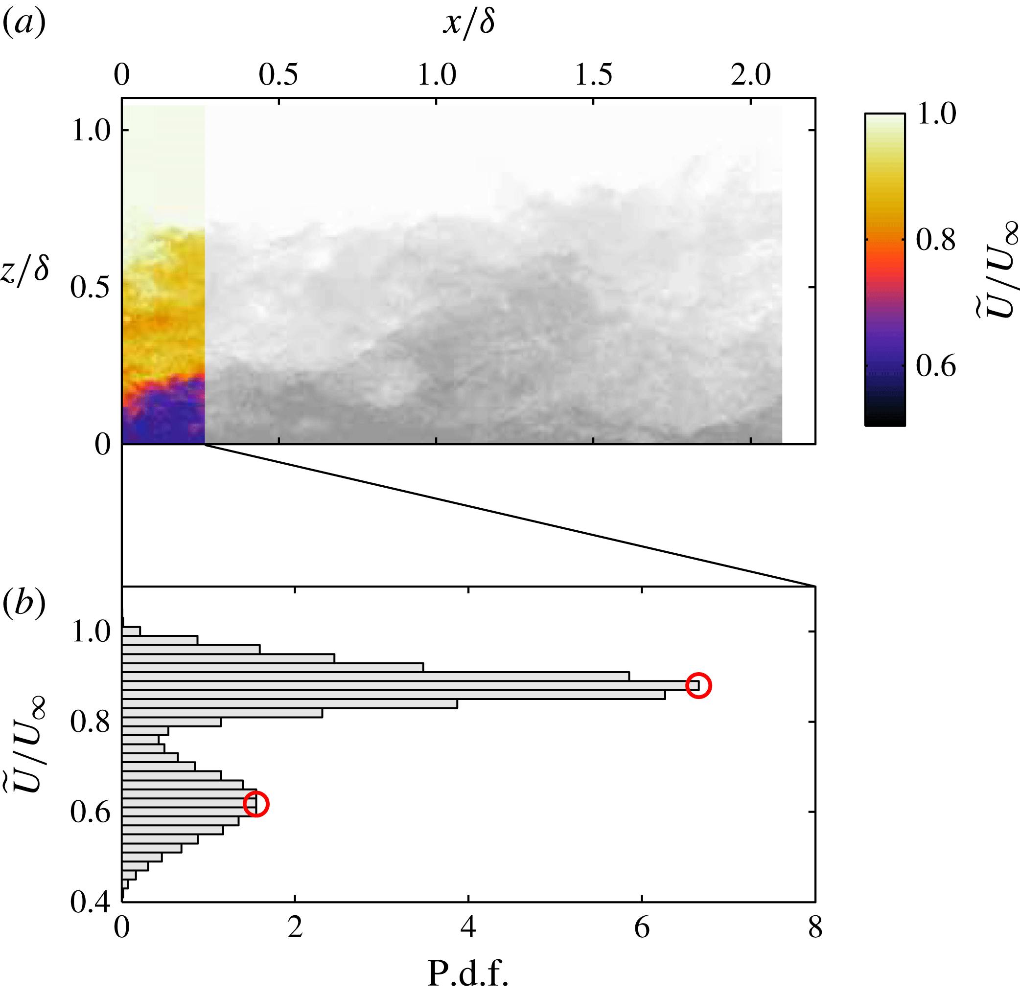
Reference Adrian, Meinhart and Tomkins2000). These local maxima are expected to be associated with the streamwise momentum of each zone, and the corresponding velocity magnitude is referred to as a modal velocity. The detection criterion employed is illustrated in figure 2, where figure 2(a) shows a sample velocity field spanning
 $2{\it\delta}$
obtained at
 $Re_{{\it\tau}}\approx 8000$
with the included region shown using colour contours on the left (i.e.
 $0\lessapprox x/{\it\delta}\lessapprox 0.25$
or up to 2000 viscous units). The corresponding histogram of the streamwise velocity in the included region is shown in figure 2(b), where the peaks of this p.d.f. correspond to possible modal velocities (
 $\widetilde{U}_{m}$
, indicated by ○ symbols). The example shows two clear peaks in the p.d.f. (modal velocities) whose corresponding UMZs are also identifiable by visually inspecting figure 2(a).
Illustration of detection criterion for UMZs applied to an instantaneous velocity field at
 $Re_{{\it\tau}}=8000$
. (a) Iso-contours of streamwise velocity (
 $\widetilde{U}$
) of the included region of a single PIV frame (colour,
 $0\lessapprox x/{\it\delta}\lessapprox 0.25$
), and omitted region in gray-scale. The colourbar for the included region is shown on the right. (b) The histogram of
 $\widetilde{U}/U_{\infty }$
constructed using the included region indicated in (a); ○ symbols indicate the detected modal velocities. The non-turbulent region is not included in constructing the p.d.f. shown in (b).

It should be noted that the non-turbulent region where
 $\widetilde{U}\approx U_{\infty }$
is not included in the p.d.f. of figure 2(b) by omitting all velocity vectors beyond the turbulent/non-turbulent interface (TNTI). The location of the TNTI is detected by employing a threshold on the kinetic energy defect (or defect in kinetic energy) of the flow (with a frame of reference moving with the free stream). Such a technique has been shown previously to work well with similar PIV data (see de Silva et al.
Reference de Silva, Philip, Chauhan, Meneveau and Marusic2013; Chauhan et al.
Reference Chauhan, Philip, de Silva, Hutchins and Marusic2014; Philip et al.
Reference Philip, Meneveau, de Silva and Marusic2014). Following Chauhan et al. (Reference Chauhan, Philip, de Silva, Hutchins and Marusic2014), the appropriate threshold is chosen by matching the intermittency profile for each dataset to other datasets (hot-wire) using an error function. This omission of velocity vectors is necessary as the strong modal velocity caused by the uniform non-turbulent region inhibits the detection of other modal velocities in the vicinity of the free-stream velocity. Further, for consistency, only the region above
 $z^{+}>100$
is included for all datasets as the velocity fields in the near-wall region are not captured by the PIV (especially for the high-
 $Re_{{\it\tau}}$
datasets).
Many investigators have measured the p.d.f. of velocities in wall-bounded flows. However, the measurements typically involved time-averaging the p.d.f. over a long period and/or averaging at only a single wall-normal location. Any of these operations will smooth out the detection of UMZs as noted by Adrian et al. (Reference Adrian, Meinhart and Tomkins2000). The streamwise length of the PIV velocity field (
 $\mathscr{L}_{x}$
) from which the p.d.f. is constructed also plays an important role. A field of view (FOV) with insufficient streamwise length for this study may lead to an insufficient number of velocity vectors (or grid points) for convergence. Meanwhile, if
 $\mathscr{L}_{x}$
is much larger than the streamwise extent of the UMZs, the local maxima (modal velocities) would tend to be smoothed out since
 $\mathscr{L}_{x}$
introduces an implicit filter on the p.d.f. We note however that a careful examination of the influence of
 $\mathscr{L}_{x}$
(and other parameters) on the number of detections shows minimal impact (see appendix A for further details). To summarise, the range utilised previously by Adrian et al. (Reference Adrian, Meinhart and Tomkins2000), where
 $\mathscr{L}_{x}\approx {\it\delta}$
(or approximately 2000 viscous units) is shown to be a reasonable choice, and therefore we will employ the same range for the subsequent analysis. However, our results show that
 $\mathscr{L}_{x}$
should be chosen based on viscous units rather than outer scaling (
 ${\it\delta}$
), as previously prescribed by Adrian et al. (Reference Adrian, Meinhart and Tomkins2000).
To elaborate further, if
 $\mathscr{L}_{x}$
is scaled on outer units (
 ${\it\delta}$
) for the high-
 $Re$
datasets,
 $L_{x}$
would be
 $O(Re_{{\it\tau}})$
, which would inhibit our ability to determine the modal velocities of UMZs associated with the smallest coherent motions (which is a viscous-dependent lower bound). Conversely, the modal velocities of larger UMZs that exceed
 $\mathscr{L}_{x}$
are readily detectable due to their large spatial signature on the velocity field. Therefore, we conclude that
 $\mathscr{L}_{x}$
should be chosen to be sufficiently small and scaled in viscous units to determine the modal velocities of the smaller UMZs (which also scale in viscous units). We note that for the lowest
 $Re_{{\it\tau}}$
dataset of Hambleton et al. (Reference Hambleton, Hutchins and Marusic2006), which does not have a streamwise FOV exceeding 2000 viscous units, we used the full streamwise extent of each instantaneous velocity field of approximately 1600 viscous units. Other important considerations include the number of bins used to form the p.d.f. and the number of velocity vectors (or grid points) available to construct the p.d.f. For consistency, both quantities are fixed for all datasets, with 50 bins and
 ${\approx}5\times 10^{3}$
velocity vectors used to construct each p.d.f. at
 $\mathscr{L}_{x}^{+}\approx 2000$
. A change in the number of velocity vectors by halving or doubling is found to have negligible effect on the computed numerical values (see appendix A) and the general conclusions are insensitive to an even bigger change.
There is a possibility that UMZs with small spatial extents may go undetected due to the
 $\mathscr{L}_{x}$
required to obtain sufficient ensembles to construct the p.d.f. As a consequence, we expect that an increase in spatial resolution may enable us to use a smaller
 $\mathscr{L}_{x}$
, while still maintaining sufficient velocity vectors to construct the p.d.f. Nevertheless, we again do not expect the conclusions drawn in this study to be sensitive to this, as will be shown quantitatively in § 4 by using a well-resolved DNS dataset at moderate
 $Re_{{\it\tau}}$
.
It is worth highlighting that a similar detection criterion was employed recently to study the uniform momentum core in turbulent channel flows, where it was shown that this region was successfully demarcated by considering the p.d.f.s of the streamwise velocity component (Kwon et al. Reference Kwon, Monty, Philip, de Silva and Hutchins2014). As a final note, when considering this type of analysis using p.d.f.s of velocity from PIV datasets, any pixel-locking (pixel displacements which are biased to integers, see Adrian & Westerweel Reference Adrian and Westerweel2011) should be carefully dealt with. A careful examination of the influence of peak locking on the detection of UMZs and how it is minimised is provided in de Silva, Hutchins & Marusic (Reference de Silva, Hutchins and Marusic2014b ). To summarise, the bias in the velocity field to integer displacements also affects the magnitude of the detected modal velocities in a similar fashion. A comparable influence of pixel-locking on modal velocities was also shown in a PIV dataset from a turbulent channel flow by Kwon et al. (Reference Kwon, Monty, Philip, de Silva and Hutchins2014). For the present analysis the degree of pixel-locking for all datasets has been checked and found to be minimal (quantified further in de Silva et al. Reference de Silva, Hutchins and Marusic2014b ).
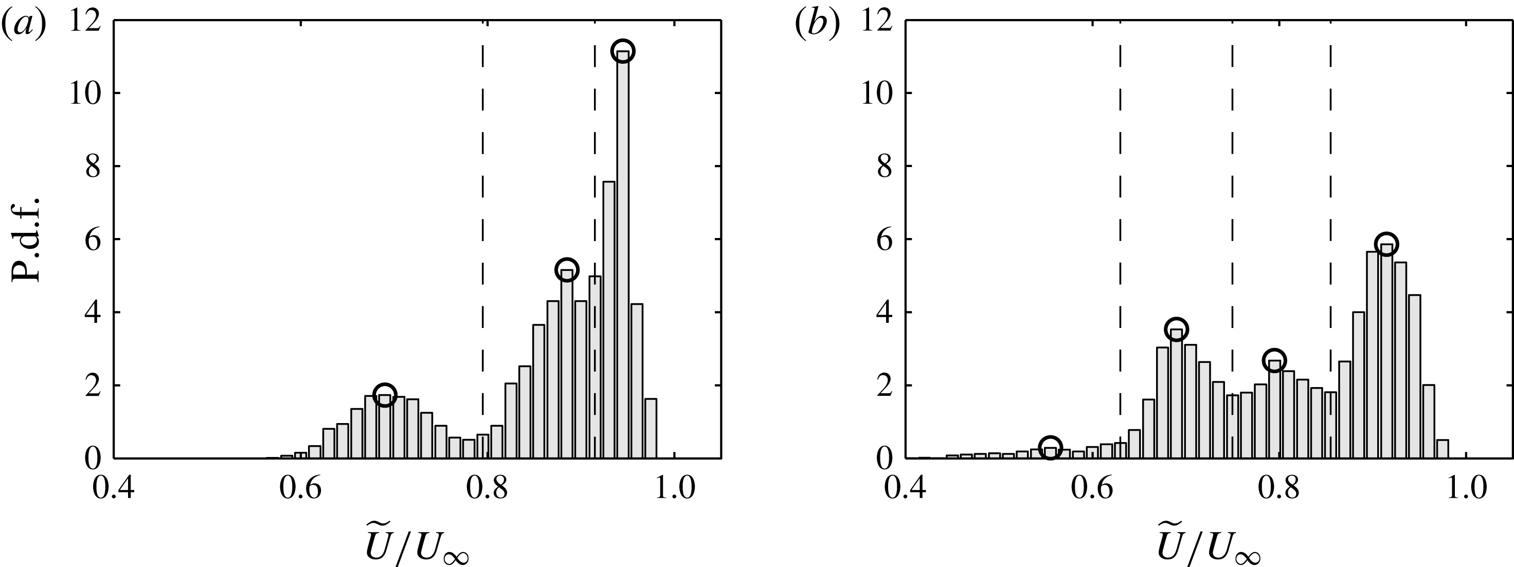
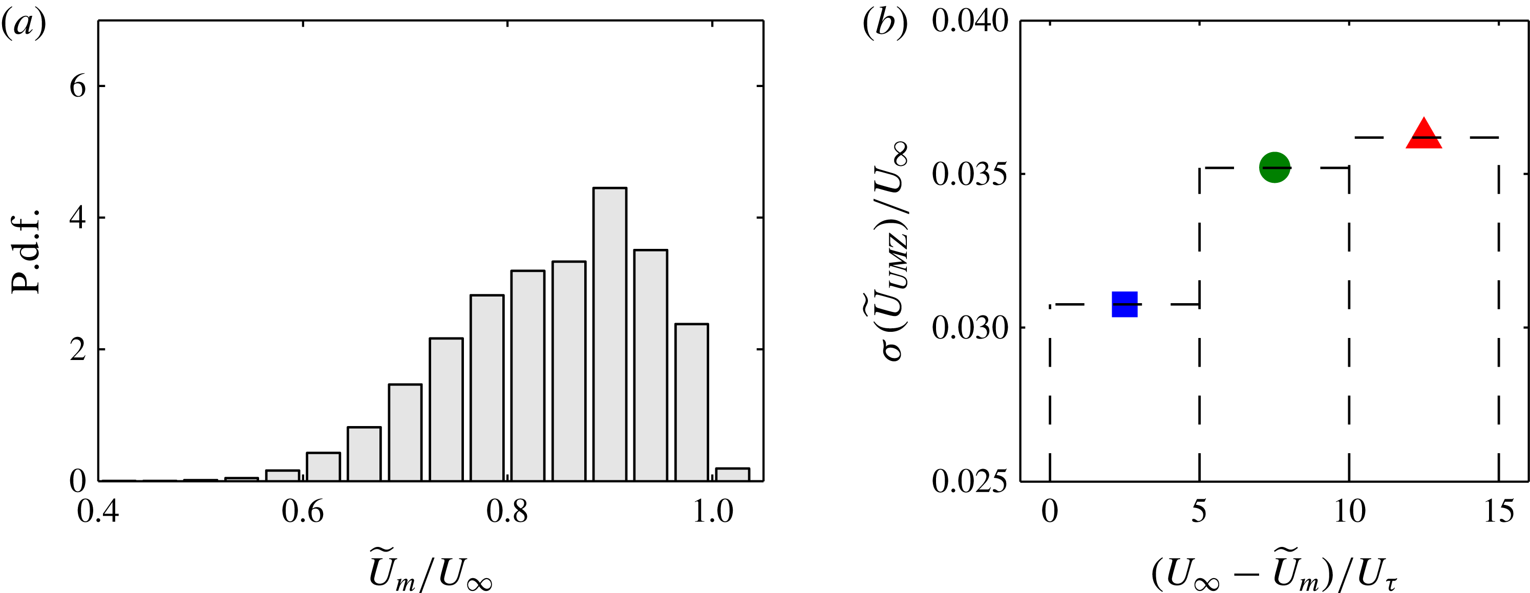
P.d.f. of the instantaneous streamwise velocity (
 $\widetilde{U}$
) normalised by
 $U_{\infty }$
at (a)
 $Re_{{\it\tau}}\approx 8000$
and (b)
 $Re_{{\it\tau}}\approx 14\,500$
. Each p.d.f. corresponds to a randomly chosen PIV frame with ○ corresponding to the detected modal velocities. The vertical dashed lines show the edges of these UMZs (mid-point of the detected modal velocities).

4. Characterisation of uniform momentum zones
In this section, we analyse the experimental databases using the detection criterion described in § 3 to explore the structural characteristics of UMZs. Figures 3(a) and 3(b) show p.d.f.s of the streamwise velocity component from randomly chosen PIV images at
 $Re_{{\it\tau}}\approx 8000$
and
 $Re_{{\it\tau}}\approx 14\,500$
, respectively with
 $\mathscr{L}_{x}^{+}\approx 2000$
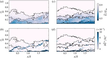
. The detected modal velocities of each UMZ are indicated by the ○ symbols, and the vertical dashed lines correspond to the streamwise velocity magnitude that separates neighbouring UMZs. For the present study, the magnitude of the streamwise velocity that demarcates each detected UMZ is approximated by the mid-point between modal velocities of neighbouring UMZs and the location of the TNTI. The corresponding instantaneous streamwise velocity field for each p.d.f. from figure 3 is shown in figure 4(a,c). The edges of each detected UMZ are represented by the solid lines, which are overlaid on colour contours of streamwise velocity. Qualitatively, it is evident that the detected edges of UMZs are accompanied by a sudden change in the streamwise velocity in the wall-normal direction (high
 $\partial \widetilde{U}/\partial z$
). We observed similar characteristics in other PIV frames from all four PIV databases, thus providing a certain degree of validity to the approach used to detect the edges of UMZs. Also noted is the presence of patches of high
 $\partial \widetilde{U}/\partial z$
along each boundary/edge (see figure 4
b,d), which show colour contours of
 $\partial \widetilde{U}/\partial z$
). Previously, Meinhart & Adrian (Reference Meinhart and Adrian1995), Adrian et al. (Reference Adrian, Meinhart and Tomkins2000) and others postulated that these patches of high
 $\partial \widetilde{U}/\partial z$
mark the possible presence of packet-like structures or vortex fissures (see Klewicki Reference Klewicki2010), where a significant proportion of the spanwise vorticity is concentrated (Priyadarshana et al.
Reference Priyadarshana, Klewicki, Treat and Foss2007). Although an interesting topic, any attempts to correlate the UMZ with vortical structure would ideally require both temporally and spatially resolved datasets. In this case the available data are more suited to an analysis of the distribution of UMZs as a function of Reynolds number.
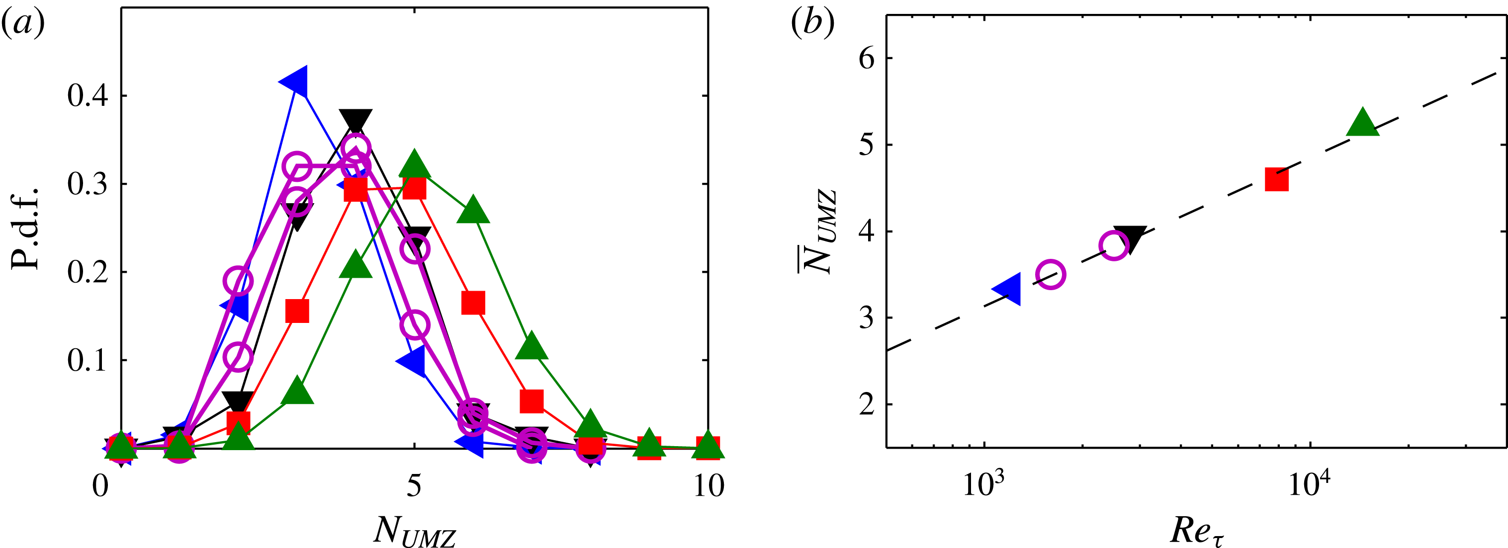
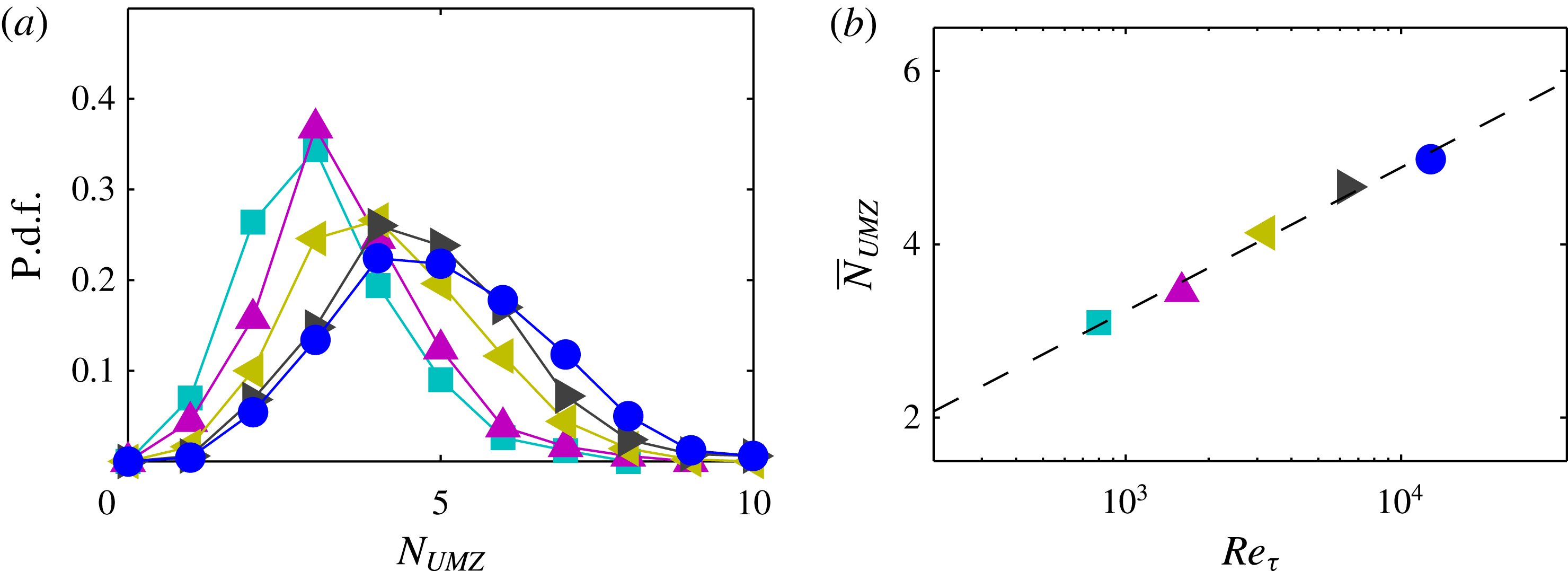
Figure 5(a) shows p.d.f.s of the number of UMZs (
 $N_{UMZ}$
) detected at various Reynolds numbers from the experimental databases. The results reveal a clear increase in
 $N_{UMZ}$
with increasing Reynolds number. Adrian et al. (Reference Adrian, Meinhart and Tomkins2000) hypothesised that the observed UMZs are caused by the presence of highly organised hairpin-like structures that form packets. If one agrees with this hypothesis, we may observe an increase in
 $N_{UMZ}$
with increasing Reynolds number as the range of scales increases. Previously, no quantitative evidence of this variation in
 $N_{UMZ}$
was observed; however, this may be caused by the limited range and magnitude of Reynolds numbers considered. The present study considers a range of Reynolds numbers that span over a decade (with sufficient scale separation), enabling us to better discern if such a trend exists.
Edges of UMZ determined using modal velocities and location of TNTI: (a,c) overlaid on colour contours of streamwise velocity (
 $\widetilde{U}$
) from a single PIV frame at
 $Re_{{\it\tau}}\approx 8000$
and
 $Re_{{\it\tau}}=14\,500$
, respectively; (b,d) overlaid on
 $\partial \widetilde{U}/\partial z$
at
 $Re_{{\it\tau}}\approx 8000$
and
 $Re_{{\it\tau}}=14\,500$
, respectively.

(a) P.d.f. of the number of UMZs detected at varying Reynolds numbers from the experimental databases: ◂, ▾, ▪, ▴ symbols correspond to datasets at
 $Re_{{\it\tau}}\approx 1200$
,
 $Re_{{\it\tau}}\approx 2800$
,
 $Re_{{\it\tau}}\approx 8000$
,
 $Re_{{\it\tau}}\approx 14\,500$
, respectively. (b) Mean number of UMZs (
 $\overline{N}_{UMZ}$
) at varying Reynolds numbers detected from the experimental databases. The ○ symbols corresponds to a recent DNS database at
 $Re_{{\it\tau}}\approx 1600$
and 2500 (Sillero, Jiménez & Moser Reference Sillero, Jiménez and Moser2013).

Figure 5(b) shows the mean
 $N_{UMZ}$
(
 $\overline{N}_{UMZ}$
) across the range of Reynolds numbers studied. The results indicate that
 $\overline{N}_{UMZ}$
has a logarithmic increase with Reynolds number (indicated by the dashed line). As will be seen in § 5, this provides strong evidence of a hierarchical length-scale distribution of structures within the boundary layer. To complement the experimental databases the ○ symbols correspond to the same analysis applied to a recent DNS database at two Reynolds numbers
 $Re_{{\it\tau}}\approx 1600$
and
 $Re_{{\it\tau}}\approx 2500$
(Sillero et al.
Reference Sillero, Jiménez and Moser2013). For the present study, 100 independent streamwise–wall-normal (
 $xz$
) planar velocity fields are extracted from the DNS databases for both Reynolds numbers. The parameters of these velocity fields are matched to the experimental database at a comparable
 $Re$
, these include: spatial domain size, resolution and velocity vector grid spacing. Furthermore, we only consider the region above
 $z^{+}>100$
, thereby matching the available region in the experimental datasets. Our analysis shows that a variation in spatial filtering and grid spacing of the DNS datasets has negligible influence on the results presented; however, for consistency it is important to omit the near-wall region (
 $z^{+}<100$
) which is unavailable in the experimental datasets. It is also worth highlighting that since these parameters are matched between the simulation and experimental databases, the p.d.f. of streamwise velocity and subsequently the performance of the detection criterion for UMZs are comparable, and are therefore not reproduced here for brevity. The results in figure 5 for the number of UMZs show good agreement between the DNS and experimental databases at a comparable Reynolds number, which further emphasises the robustness of the
 $Re$
trends observed with the experimental databases over a larger range. It should be noted that while some uncertainty remains about using modal velocities to detect UMZs and their associated boundaries, the trends with Reynolds number are robust. Additionally, based on our results, we have observed robust and qualitatively sensible detections in all PIV databases considered, which has been aided by the utility of the automated processing procedure.
The analysis to follow will employ the models described in the work of Perry and co-workers (Perry & Chong Reference Perry and Chong1982, and others) which describe the boundary layer statistics using a collection of randomly located attached eddies with a hierarchical length-scale distribution. This model provides further insight into the zonal-like structure in turbulent boundary layers observed from experimental work.
5. Revisiting the attached eddy model
The attached eddy model has been shown to reproduce flow statistics of wall-bounded turbulence reasonably well (Marusic & Perry Reference Marusic and Perry1995; Perry & Marusic Reference Perry and Marusic1995). Here, we use the model to go beyond statistics and employ it to generate synthetic instantaneous velocity fields. The synthetic velocity fields (hereafter referred to as attached eddy model (AEM) velocity fields) are generated using a structural arrangement similar to that described in Marusic (Reference Marusic2001), with hierarchies of eddies randomly distributed in groups or packets of hairpin vortices (hereafter referred to as packet-eddies). The AEM is then utilised to extract streamwise–wall-normal planes with a spatial domain and resolution equivalent to the experimental datasets investigated previously. Over 500 such planes are extracted, enabling us to calculate well-converged statistics. A brief description of the model, with emphasis placed on the generation of the synthetic velocity fields, is presented next (full details of the model can be found in Marusic & Perry Reference Marusic and Perry1995, Perry & Marusic Reference Perry and Marusic1995). For the present analysis, in addition to investigating UMZs, the AEM synthetic velocity fields prove to be a useful utility to assess the detection criterion used thus far.
5.1. Computing synthetic velocity fields from the AEM
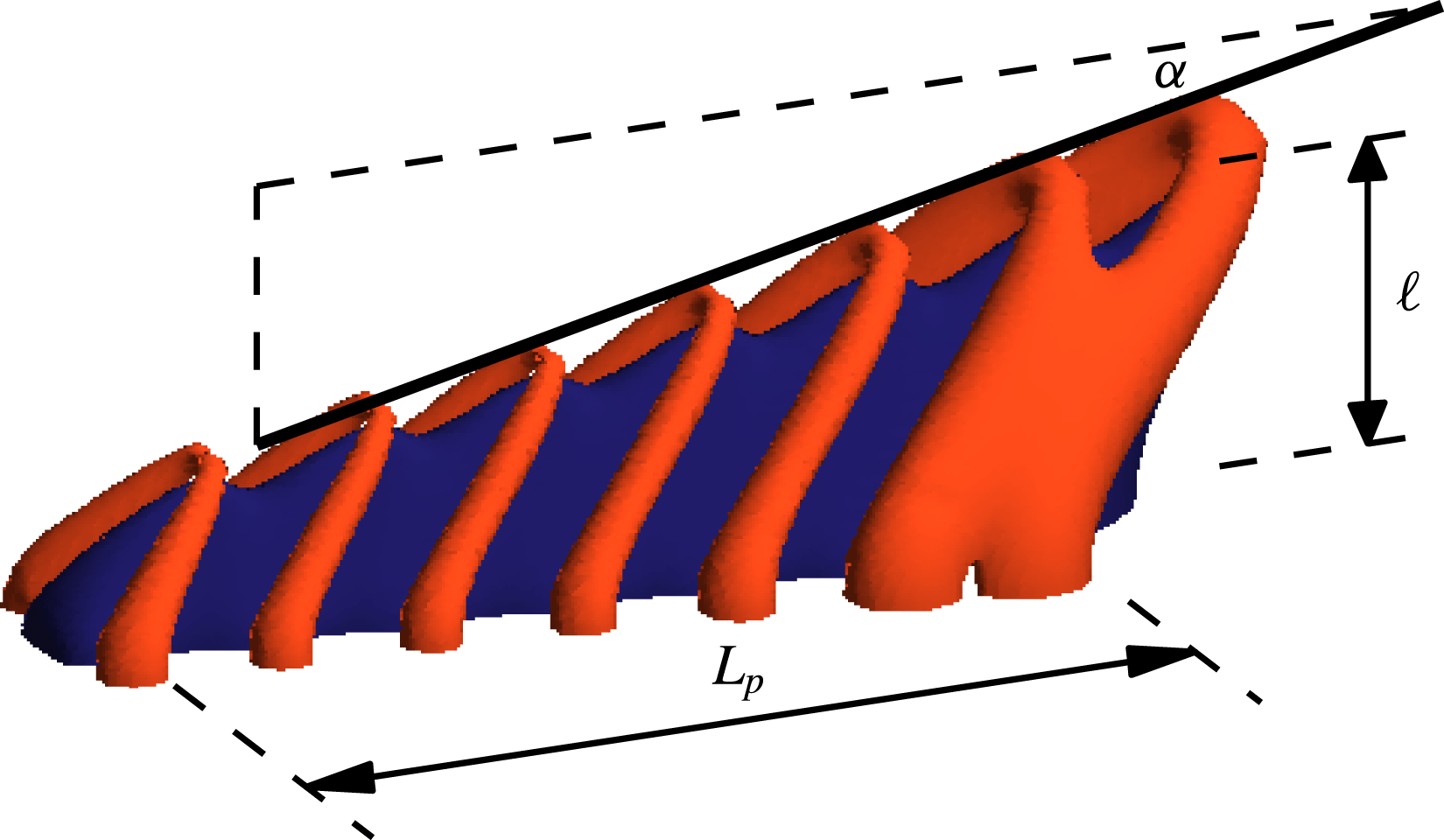
Each synthetic flow field is assumed to contain a hierarchy of packets generated from
 ${\it\Lambda}$
-eddies such as the example shown in figure 6. For the present study each representative packet-eddy consists of seven
 ${\it\Lambda}$
-eddies with an average eddy spacing of
 $0.4\ell$
(where
 $\ell$
is the wall-normal height of the largest eddy in the packet) and an inclination angle
 ${\it\alpha}=10^{\circ }$
, which are chosen based on prior work by Marusic (Reference Marusic2001). First, the velocity field for a single representative
 ${\it\Lambda}$
-eddy is computed using the Biot–Savart integral, where a Gaussian distribution of vorticity is assumed in the cores of the vortices or rods that constitute each
 ${\it\Lambda}$
-eddy (Perry & Marusic Reference Perry and Marusic1995). Thereafter, the superposition of the velocity fields from each
 ${\it\Lambda}$
-eddy within a packet (together with their image eddies in the wall) provides a representative flow field consisting of a single packet scale. This process is then repeated at different hierarchical length scales to obtain the complete AEM velocity field. The representative length scales follow a geometric progression from one hierarchy to another with self-similarity between flow fields from different hierarchies. We note that this self-similarity can be exploited to minimise the computation cost of generating AEM velocity fields, as the Biot–Savart calculations are only computed once. It should be noted that the placement of each packet-eddy in the plane of the wall is perfectly random, whereas the height of each packet-eddy follows a probability density function that adheres to the geometric progression stated in Perry et al. (Reference Perry, Henbest and Chong1986). These distributions ensure that a log law is returned for the mean flow and
 $\overline{u^{2}}$
statistics.
Schematic of a typical representative
 ${\it\Lambda}$
packet-eddy. The blue region isolates the low-momentum UMZ formed beneath the train of
 ${\it\Lambda}$
-eddies corresponding to
 ${\rm\Delta}U_{eddy}^{+}<-0.3$
; the red region corresponds to a higher speed (
 ${\rm\Delta}U_{eddy}^{+}>0.05$
). Here
 ${\it\alpha}$
is the inclination angle of the packet and
 $\ell$
is the wall-normal height of the largest eddy in the packet.
 $L_{p}$
represents the streamwise extent of the packet based on the spacing of eddies within it.

Previously, Marusic (Reference Marusic2001) established that the inclusion of representative eddies in a packet-like structure explained the velocity correlation trends observed in a turbulent boundary layer, particularly within the logarithmic region. Although not pursued by Marusic (Reference Marusic2001) it was highlighted that the reproduction of quantitatively accurate mean flow and Reynolds stresses in the turbulent boundary layer would require refinement to the shape parameters associated with the representative packet-like eddy structure. Since this study primarily focuses on UMZs in turbulent boundary layers, we will not attempt to precisely match all the Reynolds stress components for the generated synthetic velocity fields (shown previously for a non-packet-like structure, using multiple eddy shapes by Marusic & Perry Reference Marusic and Perry1995, Perry & Marusic Reference Perry and Marusic1995). Furthermore, we have not attempted to modify the model (or pursued improvements to the model) to match the experimental results; rather, we employ it as a tool to provide insight into the representative structures that are likely to be responsible for the zonal-like structure observed experimentally. However, emphasis is placed on accurately replicating the velocity deficit across the boundary layer in order to attain a comparable distribution of streamwise momentum in the AEM velocity fields similar to the experimental databases. Further details on computing the appropriate scaling and population density of the eddies for the synthetic velocity fields to attain an accurate description of the velocity deficit are provided in appendix B. To summarise, the synthetic velocity fields are scaled such that
 $\overline{uw}^{+}|_{peak}\approx 1$
in the log region, which has been empirically observed at sufficiently high Reynolds numbers. Further, the spatial population density of the eddies is chosen such that we obtain the log-law constants to match the experimental results (with
 ${\it\kappa}\approx 0.39$
and
 $A\approx 4.3$
).
For this study, synthetic velocity fields are generated spanning a large proportion of the
 $Re$
range studied experimentally from
 $Re_{{\it\tau}}=800$
to
 $Re_{{\it\tau}}=12\,800$
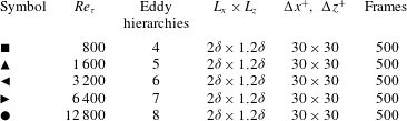
. Table 2 summarises key parameters of the AEM velocity fields. Reynolds numbers below
 $Re_{{\it\tau}}=800$
are omitted as the boundary layer is not typically considered to be fully turbulent (Klewicki, Ebner & Wu Reference Klewicki, Ebner and Wu2011). Other parameters such as the FOV and spatial resolution are closely matched to the experimental databases summarised in table 1. Following Perry and co-workers, we fix the smallest packet-eddy length scale to be on the order of
 $100{\it\nu}/U_{{\it\tau}}$
(following the Kline et al.
Reference Kline, Reynolds, Schraub and Runstadler1967 scaling), after which the number of hierarchical packet-eddies (
 $N_{h}$
) follow a geometric progression with Reynolds number.
Parameters of the attached eddy model (AEM) synthetic datasets. The number of eddy hierarchies corresponds to different energetic scales present in the AEM velocity fields at a particular
 $Re_{{\it\tau}}$
. Other parameters are defined in table 1.

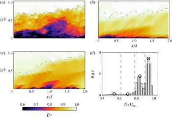
Colour contours of streamwise velocity (
 $\widetilde{U}^{+}$
) at (a)
 $Re_{{\it\tau}}\approx 8000$
from a single PIV frame, (b)
 $Re_{{\it\tau}}=6400$
from a synthetic velocity field generated using
 ${\it\Lambda}$
packet-eddies, and (c) as (b) but using
 ${\it\Pi}$
packet-eddies. The dashed line corresponds to the TNTI. (d) Figure 3 (p.d.f. of streamwise velocity,
 $\widetilde{U}/U_{\infty }$
) reproduced using the AEM velocity field shown in (b).

A few representative packet-eddy shapes are considered for this analysis, including
 ${\it\Lambda}$
-eddies,
 ${\it\Pi}$
-eddies and slanted-
 ${\it\Pi}$
eddies. Figures 7(a) and 7(b) show a qualitative comparison between an experimental velocity field at
 $Re_{{\it\tau}}\approx 8000$
and a synthetic velocity field of packets of
 ${\it\Lambda}$
-eddies at
 $Re_{{\it\tau}}=6400$
, respectively. Visual comparison between these two instantaneous velocity fields shows a reasonable degree of similarity. One notable difference is the lack of small-scale activity away from the wall for the AEM velocity fields. However, qualitative evidence of a zonal-like structural organisation within the turbulent boundary layer is easily observable, and consistent in all synthetic velocity fields generated. An examination of the p.d.f. of
 $\widetilde{U}$
(see example in figure 7
d) from the AEM synthetic velocity also shows similar evidence indicating the presence of UMZs. Figure 7(c) shows a synthetic velocity field generated using
 ${\it\Pi}$
-eddies. Although not reproduced here, the statistical behaviour of both representative packet-eddy shapes is quite similar, and therefore the subsequent analysis employs
 ${\it\Lambda}$
-eddies due to their qualitatively accurate representation of a turbulent boundary layer and geometric simplicity. Furthermore, in spite of the fact that we have considered hairpin-like structures as the representative eddy for our synthetic velocity fields, this is by no means a unique solution. In fact, we anticipate a large variety of representative eddy shapes to show both the presence of and also yield a comparable distribution of UMZs, provided the size of the energetic scales increases with distance from the wall as described in the model.
(a) P.d.f. of the number of UMZs detected in the AEM velocity fields with
 $\mathscr{L}_{x}^{+}=2000$
at varying Reynolds numbers. Symbols are defined in table 2. (b) Mean number of UMZs (
 $\overline{N}_{UMZ}$
) at varying Reynolds numbers detected in the AEM velocity fields.

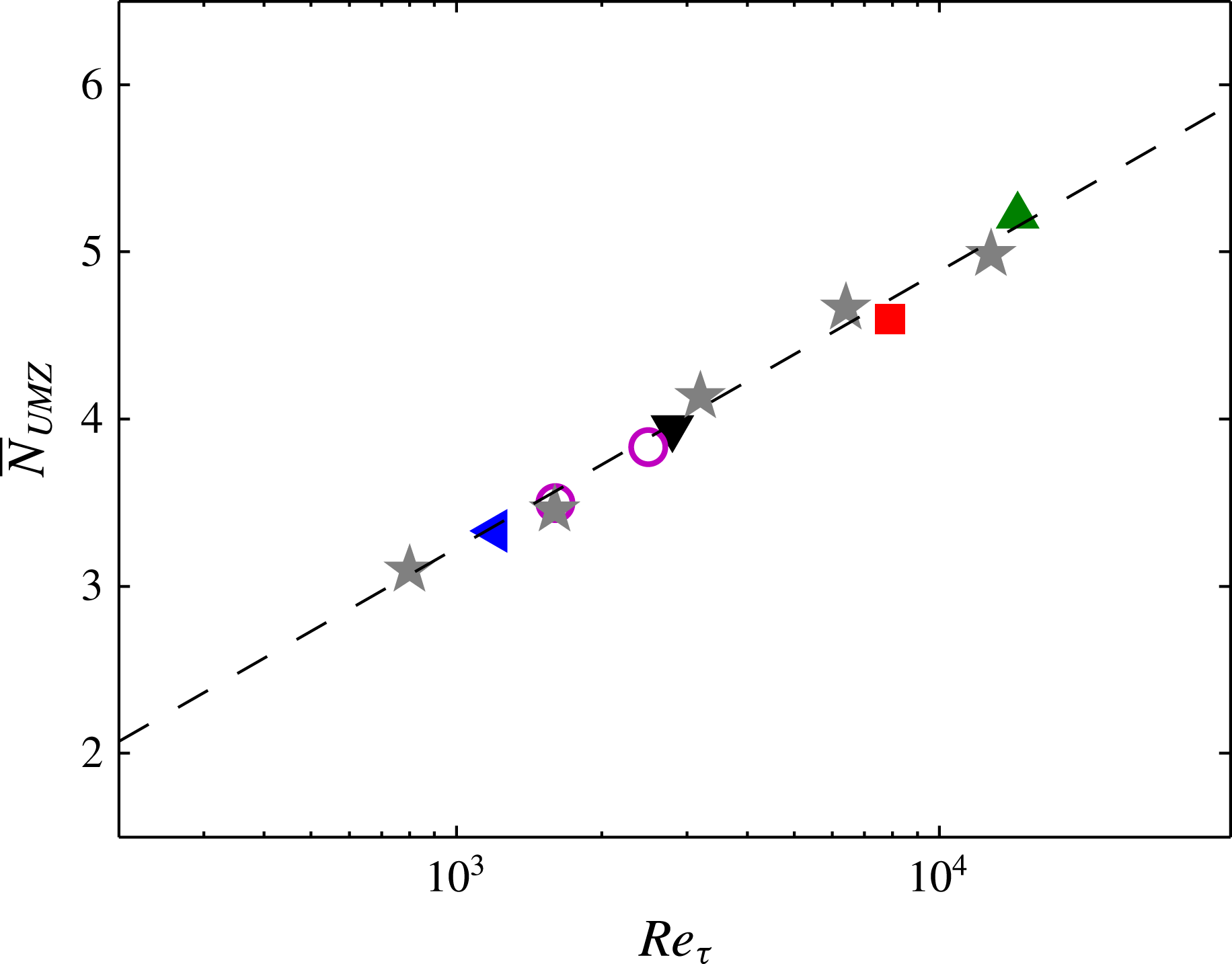
Comparison of the mean number of UMZs (
 $\overline{N}_{UMZ}$
) at varying Reynolds numbers for both the experimental data (symbols are defined in figure 5) and the AEM velocity fields (
 $\star$
symbols).

5.2. UMZs and attached eddy model
Here we use the UMZ detection algorithm described earlier for the experimental results to quantify the number and distribution of uniform momentum zones from the AEM velocity fields. Figures 8(a) and 8(b) show the p.d.f. and the mean number of UMZs (
 $\overline{N}_{UMZ}$
), respectively, from the AEM datasets. It should be noted that a fixed streamwise length of
 $\mathscr{L}_{x}\approx 2000$
is used to detect modal velocities, with the exception of the lowest
 $Re$
dataset (where
 $\mathscr{L}_{x}\approx 1600$
, due to the limited FOV). The results show that the distribution of
 $N_{UMZ}$
is quantitatively comparable to that obtained experimentally in § 4. Furthermore, our results show that
 $\overline{N}_{UMZ}$
computed from the AEM velocity fields has a logarithmic increase with Reynolds number, indicated by the dashed line on figure 8(b). Since the number of packet-eddy hierarchies has a log-linear increase with
 $Re$
, these results also indicate that the detection criterion captures the larger number of hierarchies present at higher
 $Re$
.
Figure 9 shows the average number of UMZs detected at each Reynolds number considered from both the experimental databases (coloured symbols) and the AEM synthetic datasets (
 $\star$
symbols). Results show good collapse of the observed logarithmic increase in
 $\overline{N}_{UMZ}$
with
 $Re_{{\it\tau}}$
between the experimental and AEM synthetic datasets. Consequently, we may postulate that the associated structures responsible for generating UMZs are likely to have population densities and hierarchical length-scale distributions similar to those described in the attached eddy model. This provides some insight into the representative structures that are likely to be responsible for the generation of a zonal-like structure in turbulent boundary layers.
6. Further discussion
At each Reynolds number considered,
 $N_{UMZ}$
varies for each instantaneous velocity field. One possible explanation of this variation from one instantaneous velocity field to another is the variation in the instantaneous boundary layer height (
 ${\it\delta}_{i}$
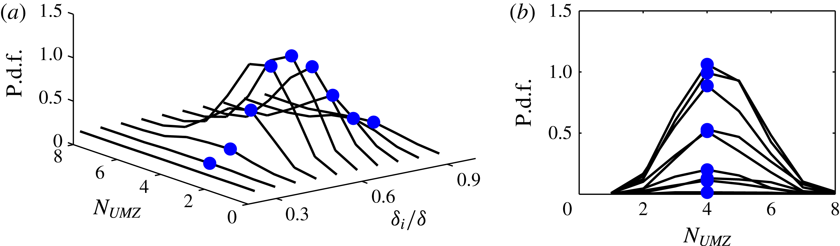
) or, equivalently, the location of the turbulent/non-turbulent interface (TNTI). To investigate this further, we consider a joint p.d.f. between
 $N_{UMZ}$
and
 ${\it\delta}_{i}$
, which is shown in figure 10 for the experimental dataset at
 $Re_{{\it\tau}}\approx 8000$
. The results show no discernible shift in the peak location (● symbols) at every contour line presented, indicating no preference of a particular
 $N_{UMZ}$
for a certain
 ${\it\delta}_{i}/{\it\delta}$
(see figure 10
b). As a consequence, one would expect the thickness of UMZs to change with
 ${\it\delta}_{i}$
. Qualitatively this result is observable on instantaneous velocity fields such as the example shown in figure 4(c) (for example, at
 $x/{\it\delta}\approx 1.5$
where
 ${\it\delta}_{i}$
is small, UMZs are observed with a reduced thickness). Similarly, at large
 ${\it\delta}_{i}$
(
 $x/{\it\delta}\approx 0.5$
) additional UMZs are not observed (instead the thickness of the UMZs seems to increase). Similar results are also observed from the other datasets, although not reproduced here for brevity.
(a) Joint p.d.f. of the number of UMZ (
 $N_{UMZ}$
) and the instantaneous boundary layer height (
 ${\it\delta}_{i}$
) at
 $Re_{{\it\tau}}\approx 8000$
. Peaks observed in each contour are indicated by ● symbols. (b) Two-dimensional projection of (a).

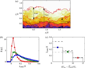
The schematic shown in figure 11(a) illustrates selected geometrical properties of UMZs. The lengths
 $z_{upper}$
and
 $z_{lower}$
indicate the upper and lower boundaries of the UMZ encapsulated by the red contour lines, and
 $t_{UMZ}$
corresponds to the thickness of the same UMZ (computed using
 $t_{UMZ}=z_{upper}-z_{lower}$
). Figure 11(b) shows a p.d.f. of
 $t_{UMZ}$
for all detected UMZs. Each colour represents UMZs that are composed of modal velocities (
 $\widetilde{U}_{m}$
) in a particular range of momentum deficit (
 $(U_{\infty }-\widetilde{U}_{m})/U_{{\it\tau}}$
). Here, we note that a larger momentum deficit can be considered to be closer to the wall (smaller
 $z^{+}$
) and vice versa. The p.d.f. of
 $t_{UMZ}$
at varying momentum deficit (wall-normal location) shows a positive skewness, which is expected since
 $t_{UMZ}$
must always be greater than zero.
(a) Parameters describing UMZ encapsulated by the red solid lines. The lengths
 $t_{UMZ}$
,
 $z_{upper}$
and
 $z_{lower}$
represent the thickness, upper and lower bounds of the UMZ, respectively. (b) P.d.f. and (c) mean of
 $t_{UMZ}$
normalised by
 ${\it\delta}$
at
 $Re_{{\it\tau}}\approx 8000$
. Results are binned by momentum deficit
 $(U_{\infty }-\widetilde{U}_{m})/U_{{\it\tau}}$
with the coloured symbols corresponding to the ranges: ▲ , 10–15; ●, 5–10; ▪, 0–5. The horizontal thick and thin dashed lines correspond to
 $\overline{t}_{UMZ}$
computed including only the top and bottom 30 % of the local boundary layer thicknesses (
 ${\it\delta}_{i}$
), respectively.

Figure 11(c) shows the mean thickness of UMZs (
 $\overline{t}_{UMZ}$
) for varying momentum deficit. Results show that as the momentum deficit of the UMZs increases (i.e. approaching the wall), the normalised UMZ thickness,
 $\overline{t}_{UMZ}/{\it\delta}$
, decreases and vice versa. This is not surprising if one subscribes to a hierarchically increasing length-scale distribution, where scales increase in size as they grow further from the wall (Townsend Reference Townsend1976; Perry & Chong Reference Perry and Chong1982; Adrian et al.
Reference Adrian, Meinhart and Tomkins2000). To further elucidate the influence of the local boundary thickness (
 ${\it\delta}_{i}$
) on
 $\overline{t}_{UMZ}$
, the horizontal thick and thin dashed lines (see figure 11
c) correspond to results computed using only the highest and lowest 30 % of
 ${\it\delta}_{i}$
wall-normal locations, respectively. The results show that an increase (or decrease) in the local boundary layer thickness (
 ${\it\delta}_{i}$
) primarily corresponds to an increases (or decrease) in thickness (
 $t_{UMZ}$
) for UMZs that reside away from the wall. Conversely, UMZs closer to the wall show no significant change in
 $t_{UMZ}$
as a function of
 ${\it\delta}_{i}$
. This observation can also be related to a structural arrangement, where one expects the wall-normal size of the larger hierarchies that reside in the outermost region of the boundary layer to predominantly influence
 ${\it\delta}_{i}$
, such as the models described in Townsend (Reference Townsend1976), Perry & Chong (Reference Perry and Chong1982), Adrian et al. (Reference Adrian, Meinhart and Tomkins2000, and others). Consequently, one would expect to associate a high
 ${\it\delta}_{i}$
with a large thickness for the UMZ furthest away from the wall and vice versa. Evidence of such a scenario is observed by examining
 $t_{UMZ}$
from the AEM datasets (figure 7
b,c). In this case it is clear that
 ${\it\delta}_{i}$
(shown by the dashed line) is primarily governed by the largest representative eddies (or hierarchies), with the smaller eddies closer to the wall having no discernible influence on
 ${\it\delta}_{i}$
. However, a more extensive examination of
 $t_{UMZ}$
inclusive of its temporal evolution would require databases that are both temporally and spatially resolved, which is unavailable in this study.
(a) P.d.f. of the modal velocities in all velocity fields at
 $Re_{{\it\tau}}\approx 8000$
. (b) Standard deviation of the streamwise turbulent fluctuations,
 ${\it\sigma}(\widetilde{U}_{UMZ})$
, normalised by free-stream velocity
 $U_{\infty }$
within each detected zone relative to the local mean of
 $\widetilde{U}$
over the spatial region of each UMZ.

Figure 12(a) shows the distribution of modal velocities (here
 $\widetilde{U}_{m}$
represents the local mean of
 $\widetilde{U}$
over the spatial extent of each UMZ) from UMZs at
 $Re_{{\it\tau}}\approx 8000$
. The results show that these regions do not have a distinctively preferred magnitude of streamwise momentum. Therefore, time averaging over a long period inhibits the observation of UMZs and their associated step-like instantaneous profiles of streamwise velocity (see figure 1); instead a smooth profile prevails. Figure 12(b) shows the standard deviation of the streamwise turbulent fluctuations in the UMZs (
 ${\it\sigma}(\widetilde{U}_{UMZ})$
) binned on momentum deficit. Therefore these results provide both a quantitative measure of the streamwise turbulence intensity within each zone and its variation with wall-normal height. However,
 ${\it\sigma}(\widetilde{U}_{UMZ})$
should be interpreted differently to the conventional turbulence intensity since it is a measure of the variation with respect to the zonal mean. The key result here is that
 ${\it\sigma}(\widetilde{U}_{UMZ})$
is fairly low, providing quantitative support for the quiescence of turbulence within each UMZ. Similar turbulence levels were also reported by Kwon et al. (Reference Kwon, Monty, Philip, de Silva and Hutchins2014) within the turbulent ‘core’ (a UMZ observed in turbulent channel flow). It should be noted that the edges of the UMZs are not omitted from the computed statistics. Therefore, one would expect, if these regions were carefully detected and removed, the uniformity within each UMZ to be even more pronounced. In future efforts, it will be valuable to consider the three-dimensional characteristics of UMZs and also report on the causality and the temporal evolution of the zonal-like arrangement, utilising datasets that are both spatially and temporarily resolved.
7. Summary and conclusions
Through the use of a large range of experimental datasets which span over a decade of
 $Re_{{\it\tau}}$
, we investigate the structural properties of the zonal-like structure observed in turbulent boundary layers. Such an analysis is made possible by the acquisition of well-resolved high-
 $Re_{{\it\tau}}$
PIV datasets with a large field of view. The study starts with an extensive examination of a detection criterion previously suggested by Adrian et al. (Reference Adrian, Meinhart and Tomkins2000) using the probability density histograms of the streamwise velocity, followed by a confirmation of prior observations in their work. This criterion is then extended to large datasets, and is shown to be capable of isolating uniform momentum zones and their associated modal velocities.
The analysis of four experimental datasets spanning over a decade of
 $Re_{{\it\tau}}$
shows a clear log-linear increase in the number of detected UMZs with increasing
 $Re_{{\it\tau}}$
. These results reveal further evidence of an hierarchical length-scale distribution of coherent structures within the boundary layer that seem to be responsible for the observed zonal-like structure. Our findings also show an increase in wall-normal thickness of UMZs further away from the wall, which agrees with the hypothesis that length scales increase in size further away from the wall. Additionally, the average number of UMZs is unchanged when conditioned on the instantaneous boundary layer height (
 ${\it\delta}_{i}$
); instead a variation in
 ${\it\delta}_{i}$
is accompanied by a change in the wall-normal thickness of UMZs that reside furthest away from the wall. Further, results show that the detected UMZs are demarcated by regions of high
 $\partial \widetilde{U}/\partial z$
(shear layers/internal boundaries). These internal boundaries show a characteristic jump in streamwise velocity similar to that observed at the TNTI (Westerweel et al.
Reference Westerweel, Fukushima, Pedersen and Hunt2005; Chauhan et al.
Reference Chauhan, Philip, de Silva, Hutchins and Marusic2014).
To complement the experimental databases utilised in this study, a range of synthetic datasets are generated by following the attached eddy models described in Marusic (Reference Marusic2001), where the boundary layer is conceived as a collection of randomly located hairpin packets. The packet-like nature of the synthetic datasets are shown to generate a zonal-like organisation similar to that observed in the experimental datasets, emphasising that the model is replicating a key structural observation from recent numerical and experimental work. Analysis of the synthetic databases again reveals a log-linear increase in the number of detected UMZs with increasing
 $Re_{{\it\tau}}$
, closely matching the trend observed from the experimental results. These results suggest that in a time-averaged sense, the UMZs appear to be well-modelled by a hierarchy of self-similar structures. Furthermore, these results appear to show that the associated structures responsible for generating these UMZs are likely to have population densities and hierarchical length-scale distributions similar to those described in the attached eddy work of Perry and co-workers.
Appendix A. Detection of UMZs — important considerations
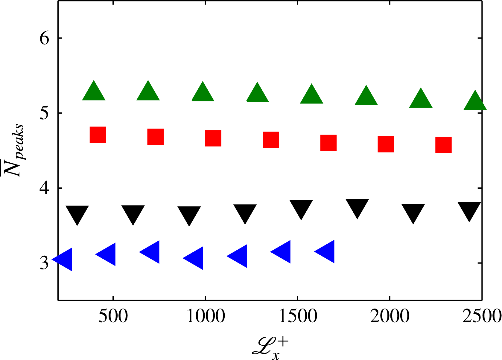
The influence of
 $\mathscr{L}_{x}^{+}$
is best illustrated with reference to figure 13, which shows the average number of peaks or modal velocities (
 $\overline{N}_{peaks}$
) detected at varying
 $\mathscr{L}_{x}^{+}$
from the experimental datasets. Since
 $\mathscr{L}_{x}$
introduces an implicit filter on the p.d.f. we would expect to observe a decrease in the number of detections at large
 $\mathscr{L}_{x}^{+}$
. However, in the range of
 $\mathscr{L}_{x}^{+}$
used for this study no significant variation in
 $\overline{N}_{peaks}$
is observed. Further, a clear increase in
 $\overline{N}_{peaks}$
with increasing
 $Re$
is evident across a range of
 $\mathscr{L}_{x}^{+}$
, showing minimal impact on the results of this study. Therefore, as previously highlighted in § 3, the range utilised previously by Adrian et al. (Reference Adrian, Meinhart and Tomkins2000) where
 $\mathscr{L}_{x}^{+}\approx 2000$
seems to be a reasonable choice, and so for this study we use a comparable
 $\mathscr{L}_{x}^{+}$
when possible. Furthermore, the range of
 $\mathscr{L}_{x}^{+}$
considered shows that either halving or doubling the number of ensembles available at
 $\mathscr{L}_{x}^{+}\approx 2000$
(achieved by simply varying
 $\mathscr{L}_{x}^{+}$
) has negligible effect on the computed
 $\overline{N}_{peaks}$
.
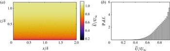
As a final note, to ensure that the detection criterion is detecting modal velocities present in a boundary layer due to the presence of coherence in the turbulence, a counter example is utilised (shown in figure 14). This synthetic velocity field is computed such that it adheres to the mean flow and turbulence intensity characteristics of a turbulent boundary layer but with the absence of any coherence in the turbulent fluctuations, thereby inhibiting the presence of UMZs (qualitatively evident in figure 14
a). Such a scenario is established by adding Gaussian white noise to the mean flow with a magnitude representative of the turbulence intensity at each wall position. The corresponding p.d.f. of the streamwise velocity is shown in figure 14(b) where it is observed that no modal velocities are present (local peaks within the boundary layer) well below
 $U_{\infty }$
. As a closing note, although the
 $Re$
trends described in this paper are robust, one may detect more or less modal velocities for a particular dataset based on the number of velocity vectors (or grid points), the
 $\mathscr{L}_{x}$
chosen or the proximity to the near-wall region. Therefore, when comparisons are drawn between datasets these parameters should be carefully considered.
Influence of
 $\mathscr{L}_{x}^{+}$
on the number of detected peaks or modal velocities: ◂, ▾, ▪, ▴ symbols correspond to datasets at
 $Re_{{\it\tau}}\approx 1200$
,
 $Re_{{\it\tau}}\approx 2800$
,
 $Re_{{\it\tau}}\approx 8000$
,
 $Re_{{\it\tau}}\approx 14\,500$
, respectively.

(a) Synthetic streamwise velocity field generated with mean flow and turbulence intensity equal to the dataset at
 $Re_{{\it\tau}}\approx 8000$
, but with no coherence in fluctuations (Gaussian white noise). (b) Corresponding p.d.f. of
 $\widetilde{U}/U_{\infty }$
from velocity field (a), where no modal velocities are observed.

Appendix B. Scaling of the synthetic velocity fields from attached eddy model
In this appendix, we outline how the synthetic velocity fields are scaled. However, first a brief description of the attached eddy formulation is warranted, to highlight the parameters associated with scaling the velocity deficit and the turbulence intensity components. Following Perry & Marusic (Reference Perry and Marusic1995) the turbulence intensity distribution can be determined by integrating over a range of length scales,
 $\ell$
, from
 ${\it\delta}_{1}$
, the smallest eddy length scale, to
 ${\it\delta}$
, the largest length scale (boundary layer thickness), by computing
 $$\begin{eqnarray}\frac{\overline{u_{i}u_{j}}}{U_{{\it\tau}}^{2}}=\frac{U_{0}^{2}}{k_{x}k_{y}}\int _{{\it\delta}_{1}}^{{\it\delta}}{\rm\Delta}(\overline{u_{i}u_{j}})\,p_{H}(\ell )\,\text{d}\ell ,\end{eqnarray}$$
where
 $p_{H}(\ell )$
corresponds to a probability distribution for each hierarchical scale (
 $p_{H}(\ell )=1/\ell$
),
 $U_{0}$
is the characteristic velocity scale of the representative eddy, and
 $k_{x}$
and
 $k_{y}$
are geometric constants where
 $k_{x}\ell$
and
 $k_{y}\ell$
are the average streamwise and spanwise spacings of the eddies in the plane of the wall.
 ${\rm\Delta}(\overline{u_{i}u_{j}})$
corresponds to the stress contribution from one scale of packet-eddies and is defined as
 $$\begin{eqnarray}{\rm\Delta}(\overline{u_{i}u_{j}})=\int _{-\infty }^{\infty }\int _{-\infty }^{\infty }\frac{\widetilde{U}_{i}\widetilde{U}_{j}}{U_{0}^{2}}\,\text{d}(x/\ell )\,\text{d}(y/\ell ).\end{eqnarray}$$
Similarly, the streamwise velocity deficit for all hierarchies can be computed by
 $$\begin{eqnarray}\frac{U_{\infty }-\overline{U}}{U_{{\it\tau}}}=\frac{U_{0}}{k_{x}k_{y}}\int _{{\it\delta}_{1}}^{{\it\delta}}{\rm\Delta}U_{eddy}(z/\ell )\,p_{H}(\ell )\,\text{d}\ell\end{eqnarray}$$
where
 ${\rm\Delta}U_{eddy}$
corresponds to the streamwise velocity contribution from one scale of representative packet-eddies and is defined as
 $$\begin{eqnarray}{\rm\Delta}U_{eddy}=\int _{-\infty }^{\infty }\int _{-\infty }^{\infty }\frac{\widetilde{U}}{U_{0}}\,\text{d}(x/\ell )\text{d}(y/\ell ).\end{eqnarray}$$
For this study, the velocity fields are scaled such that
 $\overline{uw}^{+}|_{peak}\approx 1$
in the log region, which has been empirically observed at sufficiently high Reynolds numbers. This provides us with an estimate of
 $U_{{\it\tau}}$
from (B 1) where
 $$\begin{eqnarray}\frac{\overline{uw}^{+}|_{peak}}{U_{{\it\tau}}^{2}}=\frac{U_{0}^{2}}{k_{x}k_{y}}\underbrace{\int _{{\it\delta}_{1}}^{{\it\delta}}{\rm\Delta}\overline{u_{i}u_{j}}|_{peak}\,p_{H}(\ell )\,\text{d}\ell }_{\mathscr{C}=\text{constant}}=1,\end{eqnarray}$$
and therefore
 $$\begin{eqnarray}U_{{\it\tau}}^{2}=\left.\frac{k_{x}k_{y}}{\mathscr{C}U_{0}^{2}}\,\overline{uw}^{+}\right|_{peak}.\end{eqnarray}$$
The estimate of
 $U_{{\it\tau}}$
from (B 6) can now be substituted into (B 1) to compute the other turbulence intensity components. This yields results which are independent of the population density parameters
 $k_{x}$
and
 $k_{y}$
, which cancel out. Conversely, when scaling the streamwise velocity deficit in (B 3) using the same estimate of
 $U_{{\it\tau}}$
, results are still dependent on
 $k_{x}$
and
 $k_{y}$
. Therefore, these parameters can be chosen such that the mean streamwise velocity profile in the logarithmic region satisfies
 $$\begin{eqnarray}\frac{\overline{U}}{U_{{\it\tau}}}=\frac{1}{{\it\kappa}}\log (z^{+})+A,\end{eqnarray}$$
where
 ${\it\kappa}=0.39$
(Kármán constant) and
 $A=4.3$
(log-law intersect), following Marusic et al. (Reference Marusic, Monty, Hultmark and Smits2013). However, in the present study we generate synthetic velocity fields consisting of randomly distributed packet-eddies rather than computing flow statistics from an integral form of a single representative packet-eddy ((B 1) and (B 3)). Consequently, the spatial population density (via
 $k_{x}$
and
 $k_{y}$
needs to be chosen appropriately to obtain the log-law constants (
 ${\it\kappa}\approx 0.39$
and
 $A\approx 4.3$
), and this is done by adjusting the domain size occupied by the representative packet-eddies when generating the synthetic velocity fields.