Implications
Whole-farm models are valuable tools to study the feedback and feedforward interactions between mitigation of greenhouse gas (GHG) emissions and adaptation to climate change for ruminant-based production systems. All of the processes affecting GHG emissions and farm productivity involve the cycling of C and N within the farm, most of which will be affected by climate change. However, not all farm models include such responses to climatic drivers, and there is a need for further development and testing of the models under diverse climatic conditions. Modelling of the complex interactions between farm components and the environment, including the socio-economic aspects, is instrumental for providing strategic direction to the development of climate and food-related policies. Despite the contribution of non-temperate livestock systems to total global GHG emissions, there is a dearth of specific farm models to assess GHG emissions from these regions. Modelling of soil carbon (C) fluxes is still largely absent or very simplified in many studies even though soil C has the potential to be the largest source or sink of C for grassland-based livestock systems.
Introduction
According to The Food and Agriculture Organization (FAO) (Steinfeld et al., Reference Steinfeld, Gerber, Wassenaar, Castel and De Haan2006) livestock production systems contribute about 18% of global anthropogenic greenhouse gas (GHG) emissions. Livestock is also currently one of the fastest growing agricultural subsectors in developing countries (Thornton, Reference Thornton2010), with projections indicating that by 2050 worldwide animal production is expected to increase by 80% compared with 2005 (Alexandratos and Bruinsma, Reference Alexandratos and Bruinsma2012). Although demand for non-ruminant meat has been increasing more rapidly than that for ruminant meats and, consequently, the importance of grasslands in livestock production and trade has been declining, increased milk and beef demand, potentially produced via grassland-based systems, is expected to increase (Fiala, Reference Fiala2008; Thornton, Reference Thornton2010). It is thus projected that the global annual growth rate of beef until 2050 will be 1.2%, close to the growth rate of 1.3% of total meat (Alexandratos and Bruinsma, Reference Alexandratos and Bruinsma2012). Currently, ruminant systems are a significant contributor to total livestock GHG emissions with the main sources being carbon (C) loss from land use change, methane (CH4) emissions from enteric fermentation, soil nitrous oxide (N2O) emissions and manure management.
Predictive tools and models to estimate GHG emissions from livestock systems have been developed in the form of process-based simulation (e.g. Schils et al., Reference Schils, Olesen, Del Prado and Soussana2007b), emission factor calculation (Amani and Schiefer, Reference Amani and Schiefer2011; Colomb et al., Reference Colomb, Bernoux, Bockel, Chotte, Martin, Martin-Phipps, Mousset, Tinlot and Touchemoulin2012) and life cycle assessments (LCA)-based approaches (e.g. De Vries and De Boer, Reference De Vries and de Boer2010; de Boer et al., Reference De Boer, Cederberg, Eady, Gollnow, Kristensen, Macleod, Meul, Nemecek, Phong, Thoma, van der Werf, Williams and Zonderland-Thomassen2011; Cowie et al., Reference Cowie, Eckard and Eady2012). In an effort to improve the understanding of the effect of system changes on whole farm performance and also because of the expensive, time consuming or technically difficult nature of trials at field and farm scale, whole-farm models have become more prevalent (Bryant and Snow, Reference Bryant and Snow2008). In contrast to the emission factor and LCA approaches, simulation farm models attempt to represent the flows and transformation of carbon (C) and nitrogen (N) using mechanistic processes and thus, predict resulting losses and GHG emissions.
Farm models have been developed and applied worldwide to quantify GHG emissions and to test GHG mitigation strategies (Supplementary Table S1). Farm-scale models have also been used for simulating livestock production and GHG emissions under climate change scenarios (Del Prado et al., Reference Del Prado, Shepherd, Wu, Topp, Moran, Tolkamp and Chadwick2009; Cullen and Eckard Reference Cullen and Eckard2011; Graux et al., Reference Graux, Gaurut, Agabriel, Baumont, Delagarde, Delaby and Soussana2011 and Reference Graux, Lardy, Bellocchi and Soussana2012; Bell et al., Reference Bell, Eckard and Cullen2012) that can represent a limited number of adaptation measures.
A limited number of farm-scale models also consider other ecosystem services in addition to GHG mitigation. Among the five service categories defined by MEA (2005), farm-scale models primarily cover provisioning services (food and feed), regulating services (C-sequestration, water and nutrient cycling) and supporting services (e.g. air and water pollution through ammonia volatilisation and nitrate leaching) and preservation (e.g. by improving biodiversity through set-a-side or low intensity farming). An integrated approach is needed to avoid pollution swapping when selecting among GHG mitigation options (Franks and Hadingham, Reference Franks and Hadingham2012), and farm-scale models need to consider this.
This paper complements existing reviews (Schils et al., Reference Schils, Olesen, Del Prado and Soussana2007b; Crosson et al., Reference Crosson, Shalloo, O’ Brien, Lanigan, Foley, Boland and Kenny2011; Denef et al., Reference Denef, Paustian, Archibeque, Biggar and Pape2012; Van Wijk et al., Reference Van Wijk, Rufino, Enahoro, Parsons, Silvestri, Valdivia and Herrero2012) by incorporating new topics and expanding the list of farm models reviewed. We analyse the limitations and strengths of different approaches for modelling farm-scale GHG mitigation. Even though we acknowledge that a large proportion of livestock systems and thus, GHG emissions, currently and in the future are situated in non-temperate areas (Bouwman et al., Reference Bouwman, Goldewijk, Van Der Hoek, Beusen, Van Vuuren, Willems, Rufino and Stehfest2011), because of a lack of farm models in these areas, we focused the scope of the paper on temperate grassland-based ruminant systems. The objective is to describe: basic model structures, approaches for simulating GHG emissions from different farm components, and assessing farm-scale GHG emissions and potentials for mitigation. Potential challenges for linking existing models with the simulation of impacts and adaptation measures under climate change scenarios and impacts on other ecosystem services are also explored.
Components of farm GHG models
Supplementary Figure S1 illustrates an example of the main components, inputs, outputs, material flows and emissions (e.g. C and N) from a ruminant livestock system. The flows and losses of the C and N cycle through the different farm components are affected by management and site conditions. Carbon dioxide (CO2) exchange is regulated by processes which fix C in the system and those linked with respiration or direct energy use. Methane is primarily produced in the rumen and in anaerobic storages of organic matter such as manure and silage. Atmospheric N is fixed by leguminous species, soil inorganic N is absorbed by the plant and N2O emissions are generated directly by both denitrification and nitrification processes in manure storages and soils and indirectly from N lost through ammonia (NH3) volatilisation and nitrate (NO3) leaching. GHG emissions outside of the farm boundaries (off-farm/secondary) are included in some models, such as those coming from the production of resources used, including fuel, electricity, fertiliser, pesticides, herbicides, bedding, purchased feeds and animals not produced on the farm.
Designing each of these components and integrating them into a farm model is subject to different modelling approaches in relation to the specific farm component and functionality of the model. Challenges to reduce the uncertainty of the farm model results will depend on whether the model objective is to estimate GHG emissions, assess GHG mitigation options or integrate adaptation and mitigation options.
The animal
An appropriate representation of animal metabolic processes is important to quantify how different feeding strategies and animal types affect animal productivity and excreta as well as CH4 and N2O emissions. Some models are energy-driven and animal intake is a function of the nutrient requirements of each animal group and lactation stage or production level and the nutrient constituents of the diet fed (e.g. fiber, energy and protein). Farm models generally simulate enteric CH4 using empirical models derived from statistical analyses (e.g. Olesen et al., Reference Olesen, Schelde, Weiske, Weisbjerg, Asman and Djurhuus2006; Del Prado et al., Reference Del Prado, Misselbrook, Chadwick, Hopkins, Dewhurst, Davison, Butler, Schröder and Scholefield2011a). The simplest form relates animal dry matter (DM) intake or metabolisable energy intake and CH4 output (Mills et al., Reference Mills, Kebreab, Yates, Crompton, Cammell, Dhanoa, Agnew and France2003) and others may include fatty acid profiles (Giger-Reverdin et al., Reference Giger-Reverdin, Morand-Fehr and Tran2003). Mechanistic models of rumen function are useful in understanding the dynamic processes in the rumen, but they may be too complex for integration in a farm-scale model. Farm models using empirical relationships are limited by the scope of the animal and diet characteristics used in the development of the empirical relationship (Ellis et al., Reference Ellis, Bannink, France, Kebreab and Dijkstra2010). There is thus, no agreement on the preference in the use of simpler statistical approaches over more complex mechanistic approaches (Mills et al., Reference Mills, Dijkstra, Bannink, Cammell, Kebreab and France2001).
Manure handling
Models simulate flows, losses and transformations of manure through the farm facilities, and they may simulate emissions of manure handling equipment. Models include different options or combinations of animal housing (collecting and mixing of animal excretion with water and other materials such as bedding and feed losses), manure storage (mixing manure with water), manure treatment and field application (Supplementary Table S2). Some models attempt to dynamically track the volume, DM and different fractions of C and N pools of the manure (e.g. Chardon et al., Reference Chardon, Rigolot, Baratte, Espagnol, Raison, Martin-Clouaire, Rellier, Le Gall, Dourmad, Piquemal, Leterme, Paillat, Delaby, Garcia, Peyraud, Poupa, Morvan and Faverdin2012; Olesen et al., 2006; Rotz et al., Reference Rotz, Corson, Chianese, Montes, Hafner, Jarvis and Coiner2012). For example, DM of manure can be calculated as a function of added water, added DM (e.g. straw from bedding) and an estimate of the DM of urine and dung excreted, and the inorganic N fraction from manure N can be estimated as a function of the urine : dung ratio (Rotz et al., Reference Rotz, Corson, Chianese, Montes, Hafner, Jarvis and Coiner2012). In addition, water dynamics (e.g. evaporation of water from the floor of animal housing) can be simulated as a function of the temperature in the animal facility and ventilation rate (FASSET; Hutchings et al., Reference Hutchings, Sommer and Jarvis1996).
Approaches to simulate GHG emissions and NH3 from manure range from simplified static emission factors (EF; e.g. IPCC, 2006), where emissions are predicted as an animal-based factor or a relationship of the exposed surface area and the N contained in the manure, to complex mechanistic and dynamic models of the biogeochemical processes in manure that cause the formation and emission of various compounds (Supplementary Table S1). A small number of farm models include the simulation of CO2 emissions from manure management. Methane from liquid manure storage is often modelled using the Intergovernmental Panel on Climate Change (IPCC) Tier 2 approach (IPCC, 2006) whereby CH4 output is influenced by manure volatile solids (VS), the maximum CH4 producing capacity per kilogram VS and the CH4 emission potential of manures (MCF), which is generally country-specific or can vary with temperature (Supplementary Table S1). Ammonia and N2O emissions from manure storage can also be predicted from the exposed surface each day using weather conditions, characteristics of the manure and the type of cover. When manure is removed from storage and applied to cropland, NH3 may be volatilised until the manure is incorporated into the soil and N2O emissions can follow as a function of site conditions (e.g. Rotz et al., Reference Rotz, Corson, Chianese, Montes, Hafner, Jarvis and Coiner2012) and application method (Del Prado et al., Reference Del Prado, Misselbrook, Chadwick, Hopkins, Dewhurst, Davison, Butler, Schröder and Scholefield2011a). Reference Petersen, Blanchard, Chadwick, Del Prado, Edouard, Mosquera-Losada and SommerPetersen et al. (this issue) includes a specific section on manure modelling.
Feed production
The interaction between management, soil, animal and plant genetics and weather conditions influences N2O emissions and potential soil C sequestration. Most whole-farm models only provide a representation of an average animal or plant. A limited number of models include a detailed and comprehensive representation of genes and their interactions with the environment (e.g. Hammer et al., Reference Hammer, Van Oosterom, McLean, Chapman, Broad, Harland and Muchow2010). To our knowledge, this level of detail has not been used for farm GHG emission studies, although such approaches have been used to evaluate water use efficiency (White and Snow, Reference White and Snow2012).
Approaches to simulate soil N2O emissions vary from using simple EFs which are multiplied by the total N inputs to the field to process-based models that simulate the underlying microbial processes that, through interactions with the soil physical and chemical environment, affect soil N turnover and N2O emissions (Li et al., Reference Li, Salas, Zhang, Krauter, Rotz and Mitloehner2012). The more complex models may use the ‘Hole-in-the-Pipe’ conceptual approach by Firestone and Davidson (Reference Firestone and Davidson1989), whereby the N intermediates from nitrification and denitrification processes are substrates for N2O and N2 production. The potential for N loss is calculated and then split between N2O and N2 depending on environmental factors such as temperature, water filled pore space, soil nitrate (NO3) concentration, CO2 respiration and soil porosity, which are regulated by daily temperature and rainfall patterns along with soil characteristics (Supplementary Table S1). As pulses of N2O emissions are generally driven by short-term events (e.g. rain) in combination with N substrate availability and suitable temperatures, degradable C models that represent climatic and management events will better capture the temporal variability that occurs (Chatskikh et al., Reference Chatskikh, Olesen, Berntsen, Regina and Yamulki2005).
For ruminant systems, animal grazing is an important aspect involving the simulation of direct effects and interactions between the animal, plant and animal excreta. Pasture production is generally predicted as a function of soil water and N availabilities and weather. Pasture availability can be modelled using a range in complexity from assigned empirical data (Foley et al., Reference Foley, Crosson, Lovett, Boland, O'Mara and Kenny2011) to mechanistic plant growth simulations with soil moisture, ambient temperature and solar radiation as drivers (Del Prado et al., Reference Del Prado, Misselbrook, Chadwick, Hopkins, Dewhurst, Davison, Butler, Schröder and Scholefield2011a; Rotz et al., Reference Rotz, Corson, Chianese, Montes, Hafner, Jarvis and Coiner2012). The actual amount consumed is limited to potential animal intake or the available forage, whichever is less. Remaining pasture that is not consumed may be carried over to the next time-step. Nitrogen excretion is a function of that consumed and the protein requirements of the cattle. After subtraction of NH3 volatilisation from the N deposited, the remaining N is available for plant uptake, further losses or storage in the soil. Models may include different types of grazing (e.g. continuous or rotational), although rotational grazing has proved to be more difficult to simulate for some models (e.g. Graux et al., Reference Graux, Gaurut, Agabriel, Baumont, Delagarde, Delaby and Soussana2011).
Although most pasture models are not spatial in design, that is,the pasture system is modelled as uniform across the pasture area, some do incorporate spatial variability. For example, spatial variation in urine and dung returned to the soil can be included (e.g. Hutchings et al., Reference Hutchings, Olesen, Petersen and Berntsen2007), which allows the representation of N hotspots that are more prone to directly and indirectly formed N2O emissions. In addition, paddock variations in soil properties within a farm can have a large effect on GHG emissions (Linn and Doran, Reference Linn and Doran1984; Ruser et al., Reference Ruser, Flessa, Russow, Schmidt, Buegger and Munch2006).
Soil carbon
Carbon stored in soils represents the third largest global C pool (Lal, Reference Lal2008) and grassland management methods that increase forage production have the potential to increase soil C stocks (Freibauer et al., Reference Freibauer, Rounsevell, Smith and Verhagen2004; Rees et al., Reference Rees, Bingham, Baddeley and Watson2005). Soil organic matter (SOM) dynamics and associated GHG emissions are also influenced by modifying the quality and composition of manure that is returned and more importantly, by changes in land use if animal diet changes (e.g. conversion of permanent grassland into maize (Vellinga and Hoving, Reference Vellinga and Hoving2011). Biogenic sources and sinks of CO2 are often ignored in farm GHG models with the assumption that these do not contribute to changes in atmospheric CO2 levels, that is, the source emissions equal that assimilated in sinks over the long term. However, some approaches (e.g. Rotz et al., Reference Rotz, Corson, Chianese, Montes, Hafner, Jarvis and Coiner2012) consider SOM changes and include C assimilated in crop growth and that emitted through soil, plant, animal and microbial respiration. The difference between C assimilated and emitted defines the change in soil C storage and what is exported through animal products. For long-term analyses, soil C sequestration is often negligible so that C assimilated equals that emitted plus that stored in farm produce. Changes in soil C storage occur in the short term, mainly when there is a change in land management such as conversion of rotational cropland to perennial grassland or vice versa. Following a change in land management, soil C content will seek a new equilibrium. Although soil C changes are difficult to predict at the farm scale, models are being used to predict the effects of land management on C sequestration (Del Grosso et al., Reference Del Grosso, Ojimaa, Parton, Mosier, Peterson and Schimel2002).
Other farm components
Some small-scale farmland features are not accounted for in GHG inventories such as: poached land surrounding feeding and water troughs, waterlogged areas, seepage from manures, gateways, tracks and ditches (Matthews et al., Reference Matthews, Chadwick, Retter, Blackwell and Yamulki2010). The contribution of these areas to the total farm GHG emission has been found to be generally small, although for some farms they may contribute 15% of the total GHG emission (most coming from yard seeping zones as N2O; Matthews et al.,Reference Matthews, Chadwick, Retter, Blackwell and Yamulki2010).
Other areas may be included in inventories but are generally poorly characterised such as the silage or hay production process or out-wintering and stand-off pads (enclosed areas where animals are maintained at high stocking densities and fed conserved feeds when pasture is not available or soil is too wet for grazing). Out-wintering pads or other areas where animals are kept in large densities and severe trampling occurs may create hotspots of N2O emissions derived from urine deposition (e.g. de Klein et al., Reference De Klein, Smith and Monaghan2006). Some models include simple EFs from silage effluent relating the biological oxygen demand to CH4 production (e.g. Foley et al., Reference Foley, Crosson, Lovett, Boland, O'Mara and Kenny2011; O′Brien et al., 2012a and 2012b) or relating NH3 volatilisation losses to silage DM loss (e.g. Schils et al., Reference Schils, Verhagen, Aarts, Kuikman and ŠEbek2006; Del Prado et al., Reference Del Prado, Misselbrook, Chadwick, Hopkins, Dewhurst, Davison, Butler, Schröder and Scholefield2011a). Silage effluent losses of up to 4% of the total farm emission (including secondary emissions) have been estimated (Foley et al., Reference Foley, Crosson, Lovett, Boland, O'Mara and Kenny2011). However, to our knowledge, there is no farm model that includes a mechanistic approach to these emissions at the component level as described by McGechan (Reference McGechan1990).
An economic analysis of GHG mitigation strategies is generally recommended given that the level of adoption will be predicated by the impact of these strategies on farm profitability (Foley et al., Reference Foley, Crosson, Lovett, Boland, O'Mara and Kenny2011). Furthermore, optimal adaptation to the impacts of climate change requires modelling approaches that permit financial outcomes to be explored. A number of approaches have been taken to explore the economic impacts of alternative GHG mitigation strategies (Supplementary Table S1). The value of non-market goods (e.g. animal products with increased nutritional value) and services (e.g. increased biodiversity levels) may be determined (Del Prado et al., Reference Del Prado, Misselbrook, Chadwick, Hopkins, Dewhurst, Davison, Butler, Schröder and Scholefield2011a) as some non-market attributes may eventually become valuable in monetary terms either by market pressures or regulatory-driven incentives (e.g. payments for ecosystem services). A number of studies combine bioeconomic systems models and LCA GHG emission models thus permitting the concomitant quantification of economic and GHG outcomes for alternative production scenarios (e.g. O'Brien et al., Reference O'Brien, Shalloo, Grainger, Buckley, Horan and Wallace2010; Foley et al., Reference Foley, Crosson, Lovett, Boland, O'Mara and Kenny2011). Gibbons et al. (Reference Gibbons, Ramsden and Blake2006) and Veysset et al. (Reference Veysset, Lherm and Bebin2010) combined optimisation and GHG emission models to identify cost-effective farm adaptations for reducing GHG emissions and the GHG emission impacts of farms adopting financially optimal production strategies, respectively.
Representing the interactions among farm components
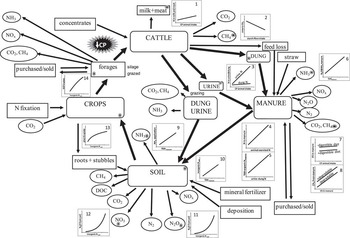
Effective evaluation of mitigation strategies requires an integrated systems approach to capture internal feedbacks and loops between farm components. Studying GHG mitigation options also requires a mass-balance approach, whereby nutrients are calculated at each time-step as the difference between inputs and outputs, and the processes at one stage depend on what happened at previous stages. Mitigation measures that benefit one farm component may affect C and N flows in other components. For example, a measure to reduce GHG emissions at the animal level may reduce CP intake and this may have large effects on the different farm components and the whole system. This can be illustrated in a conceptual diagram of C and N flows and losses for a dairy farm (Figure 1).
Conceptual diagram showing the components, pools, flows and losses of C and N that are affected after manipulation of the CP diet in a typical dairy farm. Numbered graphs illustrate one type of response that may drive the interactions between different farm variables.

The reduction of CP in the diet can directly lead to a decrease in N excretion by animals (and a reduction in manure N), but if the protein requirements of the animal are not properly met, animal productivity may suffer and emissions per unit of animal product may increase. Increasing maize in the diet led to reductions in N excretion and CH4 enteric output per litre of milk of about 6% and 14%, respectively, as simulated by a farm model (Del Prado et al., Reference Del Prado, Misselbrook, Chadwick and Newbold2011b) that used empirical equations to predict enteric production of CH4 (e.g. Mills et al., Reference Mills, Crompton and Reynolds2008). These values were in the range (8%) observed by Dijkstra et al. (Reference Dijkstra, Oenema and Bannink2011) using a mechanistic model at the rumen level. However, where such a change in feeding strategy requires land use change from pasture to maize, soil C and N losses can be much greater than animal level emissions reductions (Vellinga and Hoving, Reference Vellinga and Hoving2011).
Reducing CP may also alter the partition of N excreted resulting in a reduced ratio of urinary to dung N (Kebreab et al., Reference Kebreab, France, Beever and Castillo2001), a subsequent reduction in the ratio of total ammonium N to organic N in the manure collected and possibly a reduction in associated NH3 emissions. Manure VS, which are one of the main parameters to estimate the potential CH4 emissions from manure storage, are expected to be reduced with lower CP in the diet. Highly digestible diets, such as those rich in starch, are in general associated with higher digestibility of the excreted VS and higher CH4 losses (Hindrichsen et al., Reference Hindrichsen, Wettstein, Machmuller and Kreuzer2006).
Modelling approaches
Although mechanistic approaches may offer advantages such as increased robustness in capturing interactions and offer flexibility of use in different locations and systems, they are also sometimes too complex or difficult to parameterise at the farm scale. However, models that are mostly empirical can only provide an accurate prediction of emissions under a limited set of site and management conditions, and therefore they may be too imprecise when conditions are outside the bounds of the data used to create the model. Provided that the modeller is aware of the limitations and strengths of the approaches used, simple empirical approaches, although not universal, will be useful within the boundaries of their potential applicability.
Farm models should have sufficient complexity to satisfy their purposes (Supplementary Table S1). Most farm models include a combination of general principles and complexity in design and have been developed in a modular way integrating different existing and/or new modelling approaches. This offers advantages in flexibility and ability to incorporate new simulation capabilities, but has the potential limitation of complex model structure as well as a higher number of model parameters that need calibration. In addition, more complex models typically have a greater need for detailed data on environment (soil, climate), farm management and farm structure.
The shorter the time step, the greater the capability of the model to represent interactions between the farmer, climate and management, but this may also require more environmental and management data which is often difficult to obtain. Properly calibrated, process-based models are usually better at reproducing observed emission profiles. However, the data needed for such parameterisation is seldom available for use in whole-farm models, and simpler approaches may therefore be preferable.
Full or partial LCA, which use EFs or are integrated with simulation models, have become common tools for comprehensive assessment of GHG emissions (e.g. Beauchemin et al., Reference Beauchemin, Janzen, Little, McAllister and McGinn2010; Rotz et al., Reference Rotz, Montes and Chianese2010). Within LCA approaches, pre-chain GHG emissions from indirect land use change associated with imports of feedstuff are generally subject to large uncertainties (Weightman et al., Reference Weightman, Cottrill, Wiltshire, Kindred and Sylvester-Bradley2011).
Model evaluation and uncertainty
Irrespective of model complexity, a formal validation is rarely possible for farm-scale models since measured farm data sets are not available to ‘validate’ all or even the most important aspects of the model. Model evaluation is still very important and necessary. Individual model components must be evaluated using statistical comparisons if sufficient data exist or, if this is not possible, more qualitative comparisons of how well model predictions represent the actual farm components are necessary (e.g. Graux et al., Reference Graux, Gaurut, Agabriel, Baumont, Delagarde, Delaby and Soussana2011 for ruminant performance and CH4 emissions in pasture). When detailed farm-level data are available, a more comprehensive evaluation is possible. For example, simulated losses (N and P) and whole farm balances of N and P (Rotz et al., Reference Rotz, Oenema and Keulen2006) and plume measurement of CH4 emissions (Hensen et al., Reference Hensen, Groot, van den Bulk, Vermeulen, Olesen and Schelde2006) have been used to verify those components in whole farm simulations. When actual farm data are not available or quantifiable, the model may be best evaluated by comparing with other farm models (Schils et al., Reference Schils, de Haan, Hemmer, van den Pol-van Dasselaar, de Boer, Evers, Holshof, van Middelkoop and Zom2007a). When models developed independent of each other are found to predict similar results, this supports the validity of the models.
The uncertainty surrounding the quantification in GHG emissions from whole-farm modelling studies can be categorised according to effects of: 1. model structure, 2. model parameterisation and 3. model application, including the setup of the specific farm and the quality of the input variables needed (e.g. on livestock, soils and climate; Basset-Mens et al., Reference Basset-Mens, Kelliher, Ledgard and Cox2009). There is often a trade-off between the uncertainty associated with model complexity and that associated with model parameterisation. More complex models often have shorter time steps and include more processes, thus potentially making the results more reliable and covering the effects of more mitigation options than are possible using simpler models. However, this gives a high requirement for detailed data for model parameterisation and calibration, and model performance therefore becomes highly dependent on the quality of the data used for parameterisation (Payraudeau et al., Reference Payraudeau, van der Werf and Vertès2007). Such uncertainties within individual components may cascade within the flow chains at the farm scale, thus increasing uncertainty, in particular where the model is applied outside of its calibration range. Similar concerns also apply to models that apply simpler approaches such as EFs. These models are often more robust in their application, but they typically have lower validity outside the range for which they were constructed.
The main areas of uncertainty in GHG emissions surround N2O emissions from soils and soil organic carbon cycling (Weiss and Leip, Reference Weiss and Leip2012), whereas variation in activity data can have a considerable impact on model outcomes with respect to both productivity and emissions (Thomassen et al., Reference Thomassen, van Calker, Smits, Iepema and de Boer2008). Despite this, most whole-farm models do not represent uncertainty of simulated scenarios. However, there are some approaches that deal with variation surrounding farm system input and output parameters, and inherent uncertainties with EFs (temporal and spatial; Crosson et al., Reference Crosson, Shalloo, O’ Brien, Lanigan, Foley, Boland and Kenny2011; Stackhouse-Lawson et al., Reference Stackhouse-Lawson, Rotz, Oltjen and Mitloehner2012). Some of these studies have applied different input parameters or fixed EFs (e.g. Basset-Mens and Van der Werf, Reference Basset-Mens and van der Werf2005; Casey and Holden, Reference Casey and Holden2006; Lovett et al., Reference Lovett, Shalloo, Dillon and O'Mara2006) and then presented this as a sensitivity rather than an uncertainty analysis (Crosson et al., Reference Crosson, Shalloo, O’ Brien, Lanigan, Foley, Boland and Kenny2011). Other approaches, typically using LCA, apply Monte Carlo (MC) simulation to quantify effects of uncertainty in EFs and input variables (e.g. Gibbons et al., Reference Gibbons, Ramsden and Blake2006; Payraudeau et al., Reference Payraudeau, van der Werf and Vertès2007; Lovett et al., Reference Lovett, Shalloo, Dillon and O'Mara2008; Basset-Mens et al., Reference Basset-Mens, Kelliher, Ledgard and Cox2009; Foley et al., Reference Foley, Crosson, Lovett, Boland, O'Mara and Kenny2011). In order to carry out MC analysis, the models require information on probabilistic density functions for each sensitivity parameter. A number of models simulate weather variability to quantify variability in farm productivity levels (e.g. Graux et al., Reference Graux, Gaurut, Agabriel, Baumont, Delagarde, Delaby and Soussana2011; Belflower et al., Reference Belflower, Bernard, Gattie, Hancock, Risse and Alan Rotz2012) with consequences for GHG emissions. Uncertainties associated with emissions from different components can be easily introduced if the approaches used are accompanied by statistical information. For example, simple empirical models for CH4 output from enteric fermentation may have information on the overall error associated with the model (e.g. Mills et al., Reference Mills, Crompton and Reynolds2008). For the vast majority of farm parameters and functions, however, data are not available to determine an uncertainty range.
Assessing farm-scale GHG emissions and potentials for mitigation
Comparison of production systems
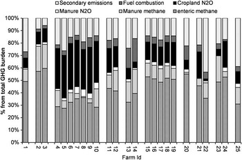
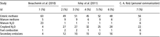
Whole-farm modelling approaches have been used to assess the GHG emissions associated with ruminant livestock production for different production systems and locations. An assessment of the relative contribution of the different sources to the absolute GHG emission is of interest to determine trends within similar production systems simulated in different locations and with different models. To illustrate the range of relative contributions of sources to the total GHG emission from dairy and beef systems, results from different studies for both dairy (Supplementary Table S2; Figure 2) and beef (Supplementary Table S3; Table 1) are shown.
Contribution of different processes to the total GHG emissions from different dairy systems. Data collected from ten different studies (Supplementary Table S2).

Contribution of different processes to the total greenhouse gas emissions from different beef systems and farm models
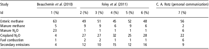
Data collected from three different studies (Supplementary Table S3).
Figure 2 shows a wide range of results. At first glance, production systems do not seem to show strong common trends. For direct site-dependent processes (e.g. manure CH4 or crop N2O), when models are considered separately, they show output sensitivity to different climatic and soil conditions (e.g. Olesen et al., Reference Olesen, Schelde, Weiske, Weisbjerg, Asman and Djurhuus2006 [Farm Ids: 4 to 10]). When comparing different models, the GHG contributions from different sources do not seem to follow any specific pattern in relation to site conditions. However, from the production systems’ viewpoint, there appears to be some pattern. For example, the inclusion of clover in the swards, sometimes as a result of conversion to organic systems, seems to result in a larger contribution from enteric CH4 (Farm Id: 2 v. 3; 13 v. 14) but smaller secondary emissions. Grazing v. confinement also resulted in a trend where larger GHG contributions were found from enteric CH4 for grazing with greater manure CH4 and secondary emissions using confinement systems.
For beef systems, it is apparent that enteric fermentation is the greatest emission source (Table 1). Of the three studies compared, Foley et al. (Reference Foley, Crosson, Lovett, Boland, O'Mara and Kenny2011) (Farm Ids: 2 to 6) had the lowest contribution from enteric fermentation largely owing to much higher levels of N fertiliser application and associated N2O emissions from soils. The higher levels of N fertiliser imported onto the farm also increased emissions from secondary sources (i.e. fertiliser production). In contrast, manure N2O emissions were much greater for Beauchemin et al. (Reference Beauchemin, Janzen, Little, McAllister and McGinn2010) (Farm Id: 1) when compared with the other two studies (Farm Id: 7). This can be attributed to the manure handling systems for the alternative beef cattle scenarios. Beauchemin et al. (Reference Beauchemin, Janzen, Little, McAllister and McGinn2010) assumed deep bedding systems were used which result in greater N2O emissions than liquid slurry systems. In contrast, the liquid slurry systems assumed in the analysis of Foley et al. (Reference Foley, Crosson, Lovett, Boland, O'Mara and Kenny2011) result in greater emission of CH4. Thus, differences in the emission sources presented in Table 1 can largely be attributed to levels of N fertiliser application and to the manure management systems used. Similar to Foley et al. (Reference Foley, Crosson, Lovett, Boland, O'Mara and Kenny2011) and Beauchemin et al. (Reference Beauchemin, Janzen, Little, McAllister and McGinn2010), Pelletier et al. (Reference Pelletier, Pirog and Rasmussen2010) showed that, regardless of production system, the cow-calf phase was the largest contributor to GHG emissions. The results showed that the pasture-based system had higher total GHG emissions than the feedlot-based system on a per unit live weight basis. Furthermore, the practice of backgrounding, that is, the period between weaning and the start of finishing, resulted in greater emissions than where progeny were sent straight to the feedlot.
Grazing v. confinement production systems
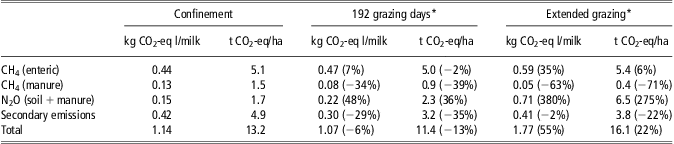
Farm models have been used to compare the GHG impacts of grazing systems compared with confinement systems (Arsenault et al., Reference Arsenault, Tyedmers and Fredeen2009; Anon, 2010; Belflower et al., Reference Belflower, Bernard, Gattie, Hancock, Risse and Alan Rotz2012; O'Brien et al., Reference O'Brien, Shalloo, Patton, Buckley, Grainger and Wallace2012a and Reference O'Brien, Shalloo, Patton, Buckley, Grainger and Wallace2012b) or gradients of replacing grazing by greater use of maize (Schils et al., Reference Schils, Olesen, Del Prado and Soussana2007b). The total effect on GHG emissions depends on whether the greater enteric emission and soil N2O emissions from grazing-based systems compared with confinement systems are counteracted by lower manure emissions. With similar milk production, greater enteric emissions from grazing-based systems is offset by lower manure emissions to provide a lower C footprint for milk produced in grazing systems (e.g. Rotz et al., Reference Rotz, Soder, Skinner, Dell, Kleinman, Schmidt and Bryant2009; O'Brien et al., Reference O'Brien, Shalloo, Patton, Buckley, Grainger and Wallace2012a and Reference O'Brien, Shalloo, Patton, Buckley, Grainger and Wallace2012b). With a much greater milk production from confinement dairies though, the C footprint of the milk produced may be similar or less than that from a grazing system (Rotz et al., Reference Rotz, Montes and Chianese2010). Other contributing factors (e.g. site conditions and intensity) or approaches have also been shown to be important. For example, in Anon (2010), three types of British intensive dairy farms were assessed for their GHG impact: 1. a confinement farm situated in a sandy loam textured location relying on grass silage, maize and a large input of concentrates; 2. a ‘conventional’ farm situated on loam textured soil relying on grazed grass (192 day grazing season) and some maize; and 3. a farm using extended grazing and concentrates located on a heavy textured soil with the importation of a large amount of mineral fertiliser. GHG emissions per litre (l) of milk were largest for the extended system and smallest for the 192 grazing day-system (Table 2). Similar to the findings of other authors (e.g. Arsenault et al., Reference Arsenault, Tyedmers and Fredeen2009), differences were smaller on a per hectare basis because of greater land use in the extended grazing systems. The main differences between confinement and extended grazing systems were because of soil N2O emissions. Although the extended grazing farm was on a soil which created greater direct N2O emissions (e.g. soil anaerobicity), the confined system, on sandy loam textured soils, had the largest NO3 leaching losses (data not shown). Results of such comparisons may therefore be highly dependent on local soil and climatic conditions.
Contribution of different processes to the total greenhouse gas emissions per litre of milk (a) and per ha (b) of three UK intensive dairy farms differing in housing production systems
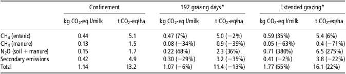
After Anon (2010).
*The emissions from the different processes for systems under 192-grazing days and extended grazing are also expressed as a relative value (%) from those emissions at the confinement system.
For both grazing and confinement systems, the modelling methodology or the assumptions taken may in fact be a large source of uncertainty in the estimation of GHG emission (Olesen et al., Reference Olesen, Schelde, Weiske, Weisbjerg, Asman and Djurhuus2006; O'Brien et al., Reference O'Brien, Shalloo, Buckley, Horan, Grainger and Wallace2011; Zehetmeier et al., Reference Zehetmeier, Baudracco, Hoffmann and Heissenhuber2012; Del Prado et al., Reference Del Prado, Mas, Pardo and Gallejones2013). For example, in studies of Zehetmeier et al. (Reference Zehetmeier, Baudracco, Hoffmann and Heissenhuber2012) and Del Prado et al. (Reference Del Prado, Mas, Pardo and Gallejones2013) large differences were found after replacing the default equation (based on IPCC Tier 2) to predict enteric CH4 emissions with alternative equations (increase of 5% to 13% total GHG when using the alternative equations) or approaches to estimate N2O emissions (increase by up to 38% total GHG when comparing the default methodology with alternative equations). Including changes in soil C would decrease/increase the total GHG burden at an average rate of 3% for each 100 kg C/ha per year stored in the soil (Del Prado et al., Reference Del Prado, Mas, Pardo and Gallejones2013).
Comparison of mitigation strategies
Some farm models have been used to test strategies to reduce GHG emissions. Del Prado et al. (Reference Del Prado, Chadwick, Cardenas, Misselbrook, Scholefield and Merino2010), for example, applied different measures and quantified the relative reduction in GHG emissions and their potential effect on pollution swapping or impact on other ecosystem services from dairy farms. Measures at the soil (nitrification inhibitors) and animal (supplementation of lipids in the diet and decreasing dietary protein) level resulted in overall reductions of at least 10% (Del Prado et al., Reference Del Prado, Chadwick, Cardenas, Misselbrook, Scholefield and Merino2010). The barriers to implementing some of these measures on real farms include relatively high costs. Reducing CP in the diet, optimising N fertilisation rate and timing and increasing frequency of reseeding would actually improve farm profit (Del Prado et al., Reference Del Prado, Chadwick, Cardenas, Misselbrook, Scholefield and Merino2010). The effect of combining five of these measures together could bring a reduction in overall GHG emission of up to 45% with most reductions caused by changes in N2O and enteric CH4. Beauchemin et al. (Reference Beauchemin, Janzen, Little, McAllister and McGinn2011), using a farm-based LCA-approach for beef systems, indicated a potential GHG emissions reduction of 20% after different combinations of measures were implemented, assuming an additive effect. Del Prado et al. (Reference Del Prado, Chadwick, Cardenas, Misselbrook, Scholefield and Merino2010), however, highlighted that the effect of combining measures is seldom additive because of the interactions in the C and N cycles on farms, already mentioned in previous sections. Moreover, after introducing more than five measures in combination, no further substantial GHG reduction was achieved (Del Prado et al., Reference Del Prado, Chadwick, Cardenas, Misselbrook, Scholefield and Merino2010). Del Prado et al. (Reference Del Prado, Chadwick, Cardenas, Misselbrook, Scholefield and Merino2010) showed that for a number of mitigation measures and under some site specific conditions, a certain level of pollution swapping could be occurring (e.g. increased NO3 or NH3 after optimisation of manure application timing). In addition, there were associated co-benefits to some ecosystem services (e.g. increased potential for biodiversity in farms through optimum fertiliser application).
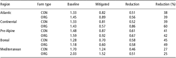
The efficiency of mitigation measures and strategies differ between farm types depending on livestock system, feeding strategies, manure handling and crop and soil management among other factors. Weiske et al. (Reference Weiske, Vabitsch, Olesen, Schelde, Michel, Friedrich and Kaltschmitt2006) studied the effects of a range of mitigation measures for conventional and organic dairy farm systems in Europe. The farms were considered to have good management, which reduced the number of mitigation options available. The most efficient mitigation options were increased lifetime efficiency of dairy cattle, use of biogas from manure digestion and improved slurry application techniques. These measures reduced emissions per litre milk by 25% to 60% (Table 3). Both the absolute emissions and the reductions varied greatly between farms, and there was no systematic difference between conventional and organic farming.
Total greenhouse gas emissions from conventional (CON) and organic (ORG) dairy farms in different European regions shown as emissions per litre milk (kg CO2-eq/l) before and after application of a set of mitigation measures that included increased lifetime efficiency of the dairy cattle, biogas of manure and improved slurry application techniques
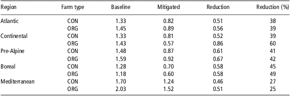
After Weiske et al. (Reference Weiske, Vabitsch, Olesen, Schelde, Michel, Friedrich and Kaltschmitt2006).
Among potential breakthrough mitigation measures, Del Prado and Scholefield (Reference Del Prado and Scholefield2008) simulated the effect on GHG emissions of introducing new traits (plants and animals), both existing and theoretical. The findings from these types of studies can provide useful guidance for breeders (Abberton et al., Reference Abberton, Marshall, Humphreys, Macduff, Collins, Marley and Donald2008; Kingston-Smith et al., Reference Kingston-Smith, Davies, Edwards and Theodorou2008). For example, improvements in the efficiency of nutrient utilisation at the plant (Del Prado and Scholefield, Reference Del Prado and Scholefield2008) and herd levels (Weiske et al., Reference Weiske, Vabitsch, Olesen, Schelde, Michel, Friedrich and Kaltschmitt2006) were shown to reduce GHG emissions per unit of animal product. Bell et al. (Reference Bell, Wall, Russell, Simm and Stott2011) also demonstrated the benefits of improved feed efficiency for dairy cows on GHG emissions per litre milk. This study used data from a long-term genetic line × feeding systems experiment to explore the impacts of genetic improvements in feed efficiency, milk production and reproductive performance on GHG emissions and land occupation. Herd dynamics were modelled using a Markov chain approach and a partial LCA was used to quantify GHG emissions. Also for dairy production systems, O'Brien et al. (Reference O'Brien, Shalloo, Buckley, Horan, Grainger and Wallace2011) used a bioeconomic farm systems model (Shalloo et al., Reference Shalloo, Dillon, Rath and Wallace2004) to simulate the effect on GHG burden of selecting cows for increased milk productivity against a selection on a combination of productivity, reproductive and health traits and found that increased milk productivity reduced GHG emissions only if reproductive and health traits are also considered.
Climate change impacts on grazing systems
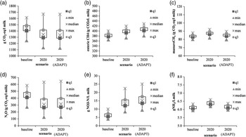
Grazing, as a production system strategy, is also expected to be affected by future climatic conditions. For example, Del Prado et al. (Reference Del Prado, Shepherd, Wu, Topp, Moran, Tolkamp and Chadwick2009) showed that UK dairy farms under projections of future climate change were more productive for most future time-slices and for most regions, mainly caused by a longer grass growing season with expected reduction of GHG emissions per unit animal product. Climate change also directly affected GHG emissions with GHG emissions sometimes being reduced (e.g. South West England in 2020; Figure 3a) mainly because of drier conditions resulting in lower mean soil N2O emissions (Figure 3d). There was an increase in overall CH4 emissions driven by lower digestibility in swards and higher temperatures for enteric and manure CH4, respectively (Figure 3b and c). Increased variability in weather events resulted in more variable GHG emissions under climate change, mainly caused by variability in soil N2O emissions (Figure 3d).
Median and range (defined by minimum, maximum and upper/lower quartiles of 30 years) of GHG emissions (a); enteric CH4 (b); manure CH4 (c), N2O emissions (d), NO3 leaching (e); and NH3 volatilisation (f) simulated results for two time-slices (baseline, and 2020s) and adapted 2020s in typical dairy farms located in south west England. After Del Prado et al. (2009).

One proposed adaptation measure was to increase the grazing period by 1 month in order to make better use of the longer growing season, which caused a modest decrease in overall net GHG, NH3 emissions and CH4 from manure. There were much larger NO3 leaching losses than in the un-adapted scenarios and slightly larger N2O emissions and enteric CH4 emissions.
Preliminary simulations with Integrated Farm System Model (IFSM) of crop and livestock production systems under projected climate change for the end of the century indicate that global warming will greatly reduce the productivity and profitability of current production practices in Pennsylvania (USA) (C. A. Rotz et al., unpublished) using current production strategies. However, by selecting alternative crop varieties and species and modifying planting and harvesting dates, etc. much, but probably not all, of the productivity and profitability can be restored.
For low-input systems such as sheep grazing in Australia, Bell et al. (Reference Bell, Eckard and Cullen2012) predicted an increase in N2O emissions caused by higher temperatures and a decrease in productivity in some situations. For warmer conditions, Bell et al. (Reference Bell, Eckard and Cullen2012) suggested replacing C3 with C4 grasses as an adaptive measure for maintaining productivity and minimising GHG emissions.
Challenges of linking GHG farm models with simulation of climate change impacts and adaptation
Policies of mitigation and adaptation are often considered in separate settings, resulting in potential conflicts. An integrated adaptation and mitigation framework is important to ensure that trade-offs between the two are minimised and synergies encouraged (Wreford et al., Reference Wreford, Moran and Adger2010). However, this is challenging as mitigation and adaptation may occur simultaneously, but differ in their spatial, timing and geographical characteristics (Smith and Olesen, Reference Smith and Olesen2010).
Process-based farm models can help prepare for the adaptation to future climate. Changes in climate and atmospheric CO2 concentration will affect plant and animal productivity but also influence GHG emissions from farming systems (Bell et al., Reference Bell, Eckard and Cullen2012). Models that simulate climate change impacts should simulate the climate-driven responses on different components of the farm. At the animal level, some models may be able to capture climatic effects on animal enteric CH4 or N excretion caused by changes in feed composition, but only a few models can include heat stress effects on animal DM intake (e.g. during grazing: Graux et al., Reference Graux, Gaurut, Agabriel, Baumont, Delagarde, Delaby and Soussana2011) and very few, to our knowledge, can simulate the effect of other climatic factors (e.g. rainfall) on animal performance (Freer et al., 2012). At the soil-plant level, C and N cycles will be influenced by changes in temperature regimes and the soil water balance. For example, increasing temperatures, when water is not limiting, are expected to accelerate SOM decomposition but result in an increase of C returns through plant residues (Bindi and Olesen, Reference Bindi and Olesen2011). Increasing SOM will increase soil C storage and may also enhance crop yield or at least improve yield stability (Pan et al., Reference Pan, Smith and Pan2009). However, biological processes resulting in N2O emissions (i.e. denitrification) could be stimulated by greater SOM. Moreover, increased variability and higher frequency of extreme events will negatively impact soil C storage, by both decreasing production levels and enhancing soil C losses. There is a lack of models that integrate these factors. Some of the effects are covered by specialised soil and crop models; however, there are few models where these are integrated at the farm level (e.g. Agricultural Production Systems sIMulator (APSIM); Keating et al., Reference Keating, Carberry, Hammer, Probert, Robertson, Holzworth, Huth, Hargreaves, Meinke, Hochman, McLean, Verburg, Snow, Dimes, Silburn, Wang, Brown, Bristow, Asseng, Chapman, McCown, Freebairn and Smith2003; EcoMod and FASSET modelling frameworks).
At the manure level, most farm models can simulate changes in direct temperature-driven emissions and sometimes indirect effects driven by changes in the composition of the feed (e.g. digestibility). However, few models can simulate the effects of short-term weather events causing N emissions after application of manure. One exception is IFSM, which simulates hourly and daily emissions following manure application as influenced by ambient temperature, soil moisture and other environmental conditions (Rotz et al., Reference Rotz, Corson, Chianese, Montes, Hafner, Jarvis and Coiner2012).
For adaptation purposes as well as for mitigation, models must include GHG emissions from secondary sources. For example, simulating enhanced cooling and ventilation systems to ameliorate animal heat stress or GHG emissions from manure storage could identify how potential adaptive measures would affect efforts to mitigate GHG emissions. Models should be able to simulate the use of similar crop rotations and pastures but adapt specified soil management practices to new conditions (e.g. irrigation, changes in fertilisation and soil cultivation, changes in grazing), or alternatively should be able to evaluate new crop rotations and pasture compositions that are more suited to the new climatic and socio-economic conditions. Furthermore, models should have enough flexibility to incorporate different realistic adaptive options and be able to study GHG mitigation measures from farming systems as affected by climatic-driven adaptive changes. Few models include the simulation of behaviour of mitigation and even fewer of adaptation (Tol, Reference Tol2005). In the case of adaptation, some models only attempt to predict the likely impacts on livestock or include adaptation measures in an arbitrary way. In both cases, models should allow estimation of economic costs or benefits incurred by these changes.
Adaptation may happen autonomously by the farmer or via policy actions. In addition, non-climate policies and regulations are already in place for other environmental issues (e.g. water quality, NH3) and therefore, models must be able to capture the effect of climatic changes on these losses as well, since the overall balance of GHG emissions may be impacted and farms may be required to adapt their nutrient management to comply with current and future regulations. For example, NO3 leaching losses are expected to increase for numerous areas that are already constrained in their nutrient use by the European Union Water Framework Directive (Jeppesen et al., Reference Jeppesen, Kronvang, Olesen, Audet, Søndergaard, Hoffmann, Andersen, Lauridsen, Liboriussen and Larsen2011). This increase in NO3 leaching may trigger more stringent regulations, and hence affect animal productivity and GHG emissions, which may also challenge climate change adaptation from a policy perspective.
For farming systems with great reliance on purchased feed (e.g. intensive beef and dairy systems), farm-scale modelling approaches must ensure some level of integration with predictive tools for estimating impacts from the land that produced the feed. Although not included in current models, there is a need to integrate the effect of climate change on plant protection issues, pollination and risks from pathogens, in particular where such effects affect the safety of livestock feed, for example, through changes in mycotoxins (Fels-Klerx et al., Reference Fels-Klerx, van der Olesen, Madsen, Uiterwijk and Goedhart2012).
Given a specific policy context, the farmer may choose among the most cost-effective and easier-to-adopt options. Ecosystem services, which currently have no market value, may also become valuable in monetary terms in the future. Therefore, some farmers may also seek to maximise the ecosystem service value as these develop a market value. There are already many studies considering these services; however, not many have focused at the farm level and more importantly, few or none to our knowledge, have the capability to quantify the potential interactions among ecosystem services both at present or in the future (Pilgrim et al., Reference Pilgrim, Macleod, Blackwell, Bol, Hogan, Chadwick, Cardenas, Misselbrook, Haygarth, Brazier, Hobbs, Hodgson, Jarvis, Dungait, Murray and Firbank2010). A balanced systems-based approach to quantify synergies and trade-offs is still lacking because of the inherent complexity of some of these relationships. Multifunctionality in farms implies greater levels of heterogeneity in farming systems, and hence increases the complexity of the farm scenarios to be modelled.
Acknowledgements
A. Del Prado would like to thank the Spanish National R+D+i Plan (grant no. CGL2009-10176) and Basque Department of Education, Universities and Research (grant no. PC2010-33A) for funding part of this study. Jørgen E. Olesen acknowledges the EU-FP7 funded AnimalChange project (grant no. 266018) for contributing to the study.
This paper was published as part of a supplement to animal, publication of which was supported by the Greenhouse Gases & Animal Agriculture Conference 2013. The papers included in this supplement were invited by the Guest Editors and have undergone the standard journal formal review process. They may be cited. The Guest Editors appointed to this supplement are R. J. Dewhurst, D. R. Chadwick, E. Charmley, N. M. Holden, D. A. Kenny, G. Lanigan, D. Moran, C. J. Newbold, P. O'Kiely, and T. Yan. The Guest Editors declare no conflict of interest.