3.1. Conservation of integral quantities

The governing equation of our system is (1.1). Multiplying by $\boldsymbol {\omega }$ and averaging, yields

(3.1)\begin{equation} \frac{\textrm{d} W}{\textrm{d} t}={-}\langle \boldsymbol{\omega} \boldsymbol{\cdot}(\boldsymbol{u} \boldsymbol{\cdot} \boldsymbol{\nabla} \boldsymbol{\omega})\rangle, \end{equation}

where $W=\langle \|\boldsymbol {\omega }\|^{2}\rangle /2$. Incompressibility allows us to write

(3.2)\begin{equation} \frac{\textrm{d} W}{\textrm{d} t}={-}\frac{1}{2} \boldsymbol{\nabla} \boldsymbol{\cdot} \langle\boldsymbol{u}\|\boldsymbol{\omega}\|^{2}\rangle, \end{equation}

and the integral of the gradient term on the right-hand side is zero for statistically homogeneous, or periodic, flows so that we obtain conservation of enstrophy,

(3.3)\begin{equation} \frac{\textrm{d} W}{\textrm{d} t}=0. \end{equation}

The proof of conservation of helicity is somewhat more involved and follows the same reasoning as in the book by Frisch (Reference Frisch1995) for the Euler equations. We need the relations,

(3.4)\begin{gather} \langle f\boldsymbol{\nabla} g\rangle ={-}\langle g\boldsymbol{\nabla} f\rangle, \end{gather}

(3.5)\begin{gather}\langle \boldsymbol{f}\boldsymbol{\cdot} \boldsymbol{\nabla} \times \boldsymbol{g}\rangle =\langle \boldsymbol{g}\boldsymbol{\cdot} \boldsymbol{\nabla} \times \boldsymbol{f}\rangle , \end{gather}

valid for arbitrary scalar fields $f,g$ and vector fields $\boldsymbol {f},\boldsymbol {g}$. Furthermore, for incompressible fields $\boldsymbol {u}$, $\boldsymbol {\omega }$, we have

(3.6)\begin{equation} \boldsymbol{\nabla}\times(\boldsymbol{u}\times \boldsymbol{\omega})=\boldsymbol{\omega}\boldsymbol{\cdot} \boldsymbol{\nabla} \boldsymbol{u}-\boldsymbol{u}\boldsymbol{\cdot} \boldsymbol{\nabla} \boldsymbol{\omega}. \end{equation}

The proof of helicity conservation goes as follows. Helicity is defined as

(3.7)\begin{equation} H={\tfrac{1}{2}} \langle \boldsymbol{\omega} \boldsymbol{\cdot} \boldsymbol{u} \rangle. \end{equation}

The evolution of $H$ is then given by

(3.8)\begin{equation} \frac{\textrm{d}H}{\textrm{d}t}={\frac{1}{2}}\left( \left\langle \frac{\partial\boldsymbol{\omega}}{\partial t} \boldsymbol{\cdot} \boldsymbol{u} \right\rangle +\left\langle \frac{\partial\boldsymbol{u}}{\partial t} \boldsymbol{\cdot} \boldsymbol{\omega} \right\rangle \right), \end{equation}

which can be written using (3.5) as

(3.9)\begin{equation} {\frac{\textrm{d}H}{\textrm{d}t}=\left\langle \frac{\partial\boldsymbol{\omega}}{\partial t} \boldsymbol{\cdot} \boldsymbol{u} \right\rangle }, \end{equation}

which avoids the need to know the equation for $\partial \boldsymbol {u}/\partial t$. Using vector identity (3.6), we can rewrite the vorticity equation (3.1) as

(3.10)\begin{equation} \frac{\partial \boldsymbol{\omega}}{\partial t}=\boldsymbol{\nabla} \times (\boldsymbol{u} \times \boldsymbol{\omega}) - (\boldsymbol{\omega} \boldsymbol{\cdot} \boldsymbol{\nabla})\boldsymbol{u}, \end{equation}

so that for the time evolution of helicity, we can write

(3.11)\begin{equation} {\frac{\textrm{d}H}{\textrm{d}t}=\left\langle \boldsymbol{u}\boldsymbol{\cdot}\boldsymbol{\nabla} \times (\boldsymbol{u} \times \boldsymbol{\omega})\right\rangle -\left\langle \boldsymbol{u}\boldsymbol{\cdot} (\boldsymbol{\omega} \boldsymbol{\cdot} \boldsymbol{\nabla} \boldsymbol{u}) \right\rangle }, \end{equation}

where both terms on the right-hand side can be shown to be zero using expressions (3.4) and (3.5) and incompressibility. We note here that this proof can be extended to the case of 2D3C flows (Biferale et al. Reference Biferale, Buzzicotti and Linkmann2017).

We note that the conservation of helicity is a global flow property in our system. For the original Euler equations, helicity is not only a global property, but is also conserved in sub-domains consisting of closed vortex tubes. The proof of this requires that forces applied to the system are irrotational (Moffatt Reference Moffatt1969). The system considered in the present investigation can be seen as the Euler equation to which we apply a force which compensates for vortex stretching at every point in space (Bos Reference Bos2021). Because the curl of this force is equal to (minus) the vortex-stretching term in the vorticity equation, it is easily observed that this force is not irrotational, and helicity in the present system is therefore not conserved in closed vortex tubes.

Strictly speaking, the enstrophy and the helicity are not the only conserved quantities. Indeed, as for 2-D turbulence, all other even powers of the vorticity, $\langle \|\boldsymbol {\omega }\|^{2n}\rangle$ are conserved by the system. Furthermore, not only the total enstrophy is conserved, but also the individual components, $\langle \omega _x^2\rangle$, $\langle \omega _y^2\rangle$ and $\langle \omega _z^2\rangle$, are conserved independently. We will consider the case where these different contributions are comparable, so that we can focus on the sum of the contributions, the total enstrophy.

3.2. Statistical equilibrium distributions

In this section, we will derive, using tools from statistical mechanics, the spectral energy distribution corresponding to thermal equilibrium of a finite set of Fourier modes. We refer to Salmon (Reference Salmon1998) and Thalabard (Reference Thalabard2013) for detailed derivations using the present approach. We consider that the flow is decomposed on a finite number $N$ of Fourier components $\boldsymbol {u}(\boldsymbol {k})$. The vector space $\boldsymbol {k}$ is thus decomposed by its coordinates $\boldsymbol {k}_n$, with $n=1,\ldots,N$. Note that in this section, the subscript $n$ does not indicate a vector index, but simply a counter. The value $N$ corresponds to the total number of modes. This means that in a 3-D cubic domain with $N_{k_x}$ modes in each direction, $N=N_{k_x}^3$. Note that the Fourier coefficients of velocity satisfy the conjugate symmetry $\boldsymbol {u}(\boldsymbol {k})=\boldsymbol {u}^*(-\boldsymbol {k})$, because the velocity is a real quantity in physical space, thus the total number of independent degrees of freedoms of the system is $N/2$.

We consider incompressible flow, where the divergence in Fourier space implies $\boldsymbol {k}\boldsymbol {\cdot } \boldsymbol {u}(\boldsymbol {k})=0$, so that only two independent Fourier coefficients are needed to represent the velocity vector $\boldsymbol {u}(\boldsymbol {k}_n)$. Because, in addition, the Fourier coefficients are complex, a total of four independent real coefficients describe each mode. These modes are denoted $y_{n_1}, y_{n_2}, y_{n_3}, y_{n_4}$, where $n$ is from $1$ to $N$. In total therefore, if we have $N$ wave-vector coordinates representing a 3-D velocity field, we have to consider the dynamics of a system of $4N$ coordinates in phase space. A convenient way to choose the independent modes will be described now.

Following Waleffe (Reference Waleffe1992), Cambon & Jacquin (Reference Cambon and Jacquin1989) and Kraichnan (Reference Kraichnan1973), we represent the velocity field of an incompressible 3-D fluid by using a helical-mode decomposition. Every 3-D Fourier vector $\boldsymbol {u}(\boldsymbol {k})$ can be represented by two orthogonal complex helical waves $\boldsymbol {h}^{\pm }=\hat {\boldsymbol {w}}\times \hat {\boldsymbol {k}}\pm \mathrm {i}\hat {\boldsymbol {w}}$ with $\hat {\boldsymbol {k}}=\boldsymbol {k}/k$ the unit vector parallel to $\boldsymbol {k}$. Here, the unit vector $\hat {\boldsymbol {w}}$ can be chosen as $\hat {\boldsymbol {w}}=\boldsymbol {z}\times \boldsymbol {k}/|\boldsymbol {z}\times \boldsymbol {k}|$ for an arbitrary vector $\boldsymbol {z}$. It then follows that

(3.12)\begin{equation} \boldsymbol{u}(\boldsymbol{k})=u^+(\boldsymbol{k})\boldsymbol{h}^+(\boldsymbol{k})+u^-(\boldsymbol{k})\boldsymbol{h}^-(\boldsymbol{k}). \end{equation}

Note that $u^+(\boldsymbol {k})$ and $u^-(\boldsymbol {k})$ are complex numbers.

As stated above, all coordinates $\boldsymbol {k}$ of the considered part of Fourier space are individually labelled $\boldsymbol {k}_n$, with $n$ ranging from $1$ to $N$. Because at each coordinate $\boldsymbol {k}_n$ we have four individual real coefficients $y_{n_1}, y_{n_2}, y_{n_3}, y_{n_4}$, we can thus define using the following representation:

(3.13)\begin{equation} \left. \begin{gathered} y_{n_1}=\mathrm{Re}(u^+(\boldsymbol{k}_n)),\quad y_{n_2}=\mathrm{Im}(u^+(\boldsymbol{k}_n)),\\ y_{n_3}=\mathrm{Re}(u^-(\boldsymbol{k}_n)),\quad y_{n_4}=\mathrm{Im}(u^-(\boldsymbol{k}_n)). \end{gathered} \right\} \end{equation}

The main motivation to use the helical mode decomposition in the present investigation is that we have a simple relation between the generalized coordinates and the modal energy, helicity and enstrophy,

(3.14)\begin{align} \tfrac{1}{2} \boldsymbol {u}(\boldsymbol{k}) \boldsymbol{\cdot} \boldsymbol {u}^{*}(\boldsymbol{k})&=u_{+} u_{+}^{*}+u_{-} u_{-}^{*}\nonumber\\ &=y_{n_1}^2+y_{n_2}^2+y_{n_3}^2+y_{n_4}^2=E_n, \end{align}

(3.15)\begin{align} \tfrac{1}{2} \boldsymbol{u}(\boldsymbol{k}) \boldsymbol{\cdot} \boldsymbol{\omega}^{*}(\boldsymbol{k})&=\left(u_{+} u_{+}^{*}-u_{-} u_{-}^{*}\right)\nonumber\\ &=|\boldsymbol{k}_n|\left(y_{n_1}^2+y_{n_2}^2-y_{n_3}^2-y_{n_4}^2\right)=H_n, \end{align}

(3.16)\begin{align} \tfrac{1}{2} \boldsymbol{\omega}(\boldsymbol{k}) \boldsymbol{\cdot} \boldsymbol{\omega}^{*}(\boldsymbol{k})&=k^2(u_{+} u_{+}^{*}+u_{-} u_{-}^{*})\nonumber\\ &=|\boldsymbol{k}_n|^2(y_{n_1}^2+y_{n_2}^2+y_{n_3}^2+y_{n_4}^2)=W_n. \end{align}

In the following, we will use that all four coefficients $y_n$ correspond to the same position in Fourier space so that we can write $|\boldsymbol {k}_n|=k$. Now that we have defined the invariants as a function of the generalized coordinates $y_{n_i}$ in phase space, we can proceed with the derivation of the equilibrium distribution.

The fundamental principle of equilibrium statistical mechanics states that in systems satisfying a Liouville equation (non-divergent evolution of the generalized coordinates), the probability density $P(\boldsymbol {y})$ eventually becomes uniform over all accessible parts of phase space (Salmon Reference Salmon1998). We will compute the average spectral energy distribution associated with this thermal equilibrium state. An essential ingredient to compute the average corresponding to this distribution is the probability density. The partial density, or partition function for mode $n$, $P_{n}(y_{n_1},\ldots,y_{n_4})$, is considered to satisfy a Boltzmann–Gibbs equilibrium distribution,

(3.17)\begin{equation} P_{n}\left(y_{n_1},\ldots,y_{n_4}\right)= C_{n} \exp \left[{-}S_n\right], \end{equation}

where $S_n$ is a function of the constants of motion and $C_n$ is a constant. For instance, if enstrophy and helicity are conserved, as in our case, the quantity $S_n$ writes

(3.18)\begin{equation} S_n=\alpha W_{n}+\beta H_{n}, \end{equation}

where $\alpha$ and $\beta$ are Lagrange multipliers representing some kind of inverse statistical temperature or chemical potential. The function $P_n$ gives thus the probability to find values $y_{n_i}$ for mode $n$. It is at this point that the approach of different physical systems is distinct. For 2-D turbulence, $W_n$ and the energy $E_n$ would appear, whereas in classical 3-D turbulence, $E_n$ and $H_n$ would appear in expression (3.18).

We have thus, substituting definitions (3.15) and (3.16) in (3.17),

(3.19)\begin{align} P_{n}\left(y_{n_1},\ldots,y_{n_4}\right) & = C_{n} \exp \left[({-}k^2\alpha-k\beta)(y_{n_1}^2+y_{n_2}^2)\right.\nonumber\\& \quad + \left.({-}k^2\alpha +k\beta)(y_{n_3}^2+y_{n_4}^2) \right]. \end{align}

We define $Z_n$ the integral of $P_n$,

(3.20)\begin{equation} Z_n=\iiiint P_n \,\mathrm{d}y_{n_1}\,\mathrm{d}y_{n_2}\,\mathrm{d} y_{n_3}\,\mathrm{d} y_{n_4}. \end{equation}

The average enstrophy per mode is given by

(3.21)\begin{align} \langle W_n\rangle &=\sum_{i=1,\ldots,4}\langle k^2 y_{n_i}y_{n_i}\rangle \end{align}

(3.22)\begin{align} &=\sum_{i=1,\ldots,4}\frac{1}{Z_n}\iiiint \left[k^2 P_n y_{n_i}y_{n_i}\right]\,\mathrm{d}y_{n_1}\,\mathrm{d} y_{n_2}\,\mathrm{d}y_{n_3}\,\mathrm{d}y_{n_4}. \end{align}

From (3.17) and (3.20) it is observed that we can compute the average directly using

(3.23)\begin{equation} -\frac{1}{Z_n}\frac{\partial Z_n}{\partial \alpha} =\langle W_n\rangle, \end{equation}

and similarly

(3.24)\begin{equation} -\frac{1}{Z_n}\frac{\partial Z_n}{\partial \beta} =\langle H_n\rangle. \end{equation}

The integral (3.20) can be computed to yield

(3.25)\begin{equation} Z_n =\frac{{\rm \pi}^2}{k^4\alpha^2-k^2\beta^2}, \end{equation}

so that we find for the enstrophy and helicity,

(3.26a,b)\begin{equation} \langle W_n \rangle=\frac{2\alpha k^2}{\alpha^2 k^2 - \beta^2}, \quad \langle H_n\rangle=\frac{2\beta}{\alpha^2 k^2 - \beta^2}. \end{equation}

The enstrophy spectrum and helicity spectrum are therefore, owing to isotropy,

(3.27a,b)\begin{equation} W(k)=\frac{8{\rm \pi}\alpha k^4}{\alpha^2 k^2 - \beta^2}, \quad H(k)=\frac{8{\rm \pi}\beta k^2}{\alpha^2 k^2 - \beta^2}, \end{equation}

so that the kinetic energy spectrum writes

(3.28)\begin{equation} E(k)=\frac{8{\rm \pi}\alpha k^2}{\alpha^2 k^2 - \beta^2}. \end{equation}

This last expression is the principal theoretical result of the present investigation. An important feature of this expression, in contrast to expression (2.5) derived for classical turbulence, is that in the present case, helicity does mainly affect the large scales. Expression (3.28) and its implications will be verified using simulations.

3.3. Integral relations between the enstrophy, helicity and energy for the equilibrium distributions

Because the enstrophy and helicity are conserved quantities of the system, the statistical characterization of our system in statistical equilibrium is completely determined by the values of the enstrophy and helicity,

(3.29a,b)\begin{equation} W=\int_{k_{min}}^{k_{max}}k^2E(k)\,\mathrm{d}\kern0.09em k,\quad H=\int_{k_{min}}^{k_{max}}H(k)\,\mathrm{d}\kern0.09em k, \end{equation}

as soon as we know $k_{min}$ and $k_{max}$ and the initial conditions. Indeed, the unknown coefficients $\alpha$ and $\beta$ in the equilibrium spectra are fully determined by the other parameters. This allows us to predict the expected long time value of the kinetic energy

(3.30)\begin{equation} E=\int_{k_{min}}^{k_{max}}E(k)\,\mathrm{d}\kern0.09em k, \end{equation}

as a function of the enstrophy and helicity. Let us illustrate this for the simplest, mirror-symmetric case. For that case, we have $\beta =0$, which leads to

(3.31)\begin{equation} W=\int_{k_{min}}^{k_{max}}8 {\rm \pi}\frac{k^2 }{\alpha}{\rm d}\kern0.06em k\, \approx \frac{8{\rm \pi}}{3}\frac{k_{max}^3}{\alpha}, \end{equation}

which allows us to express $\alpha$ as a function of $W$ and $k_{max}$, where we used that $k_{min}\ll k_{max}$. Substituting this in the kinetic energy spectrum and integrating yields

(3.32)\begin{equation} E\approx 3\frac{W}{k_{max}^2}, \end{equation}

so that we have a prediction for the final value of the kinetic energy as a function of the initial condition for $W$. When both helicity and enstrophy are non-zero, the computation becomes more tedious, but can still be performed analytically. We introduce the ratio $\gamma =\beta /\alpha$ so that the helicity spectrum writes

(3.33)\begin{equation} H(k)=\frac{ 8 {\rm \pi}\gamma}{\alpha} \frac{ k^2}{k^2-\gamma^{2}}. \end{equation}

For this expression to make sense, the minimum wavenumber should verify $k_{min}>\gamma$. Under this constraint, we can integrate the helicity spectrum to obtain the expression

(3.34)\begin{equation} H=\frac{ 8 {\rm \pi}\gamma}{\alpha}\left(k_{max}-k_{min}+\frac{\gamma}{2}\ln\left(\frac{k_{max}^2-\gamma^2}{k_{min}^2-\gamma^2}\right) \right), \end{equation}

which relates the helicity to $k_{max}$, $k_{min}$, $\alpha$ and $\beta$. For the helical cases, the relation between energy and helicity is simply $E= H/ \gamma$.

5.1. Conservation of enstrophy and helicity during relaxation

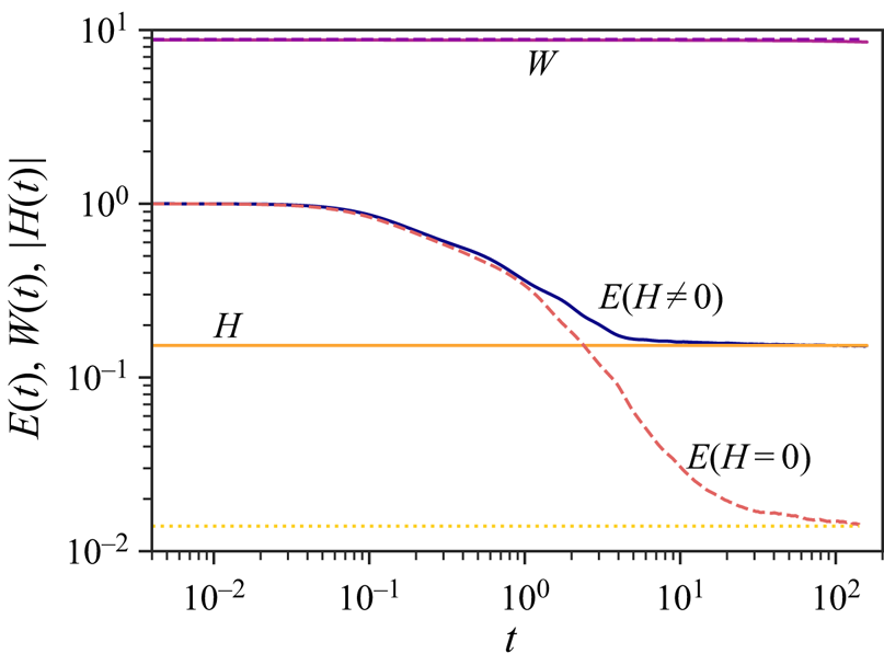
In figure 2, we show the time evolution of enstrophy, helicity and kinetic energy. Note that the initial energy $E_0$ is unity. Time is normalized by a characteristic time scale $\tau =1/\sqrt {E_0 k_{min}^2}$. For the case of mirror-symmetric truncated Euler turbulence without vortex stretching, a clear conservation of enstrophy is observed, whereas the kinetic energy decays. Helicity remains negligible throughout the simulation. The prediction of the kinetic energy, discussed in § 3.3, is represented by a dotted line. It is observed that the expected steady state is reached for the kinetic energy. This steady state is the predicted equilibrium state, where the Fourier modes all contain, on average, the same amount of enstrophy.

Figure 2.

Time evolution of energy, enstrophy and helicity for the inviscid, force-free, 3-D, no vortex-stretching turbulence: solid lines, helical case; dashed lines, mirror-symmetric case; dotted line, the analytical prediction of the kinetic energy for the mirror-symmetric case.

In figure 2, the same results are also plotted for the helical case. It is observed, as shown in our proof (§ 3.1), that helicity is conserved by the system. As mentioned in § 3.3, the prediction of the final kinetic energy in the helical case is $E= H/ \gamma$. After calculation, we have $\gamma =-0.9989\approx -1$ in our simulation. This corresponds to the observation that the kinetic energy tends to the absolute value of the helicity. This tendency is not a coincidence, but reflects the condensation of energy into a helical flow structure at scales with wavenumber $k=1$, as will be shown next. It is also shown that the presence of helicity allows the flow to retain more kinetic energy in the system than the mirror-symmetric case does. Indeed, without helicity, the energy drops to less than $2\,\%$ of its initial value, while in the helical case, this value is approximately $15\,\%$.

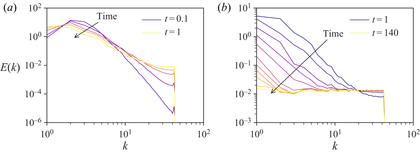
To further investigate the dynamics of the truncated system, we show in figure 3(a,b) the evolution of the kinetic energy spectra towards the equilibrium state. It is observed that enstrophy accumulates rapidly at the largest spatial frequencies, in a similar manner as energy accumulates in classical truncated Euler dynamics (Cichowlas et al. Reference Cichowlas, Bonaïti, Debbasch and Brachet2005; Bos & Bertoglio Reference Bos and Bertoglio2006). This evolution was correctly predicted and explained by Bos (Reference Bos2021).

Figure 3.

Inviscid relaxation for helicity-free turbulence: (a) short time evolution, showing the kinetic energy spectra at $t$ = 0.1, 0.2,0.4, 0.6, 1; (b) long time evolution, showing the spectra at $t$ = 1, 2, 4, 6, 10, 20, 40, 60, 100, 120, 140.

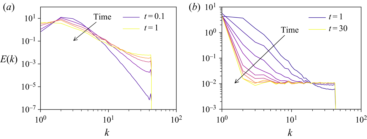
The dynamics of the helical case (figure 4a,b) is quite similar, except for the persistent energy at the smallest wavenumbers. This is anticipated by the statistical mechanics predictions in § 3 and we will focus on them now.

Figure 4.

Inviscid relaxation for helical turbulence: (a) Short time evolution, showing the kinetic energy spectra at $t$ = 0.1, 0.2, 0.4, 0.6, 1; (b) long time evolution, showing the spectra at $t$ = 1, 2, 4, 6, 8, 10, 14, 16, 18, 30.

5.2. Comparison with predicted shapes

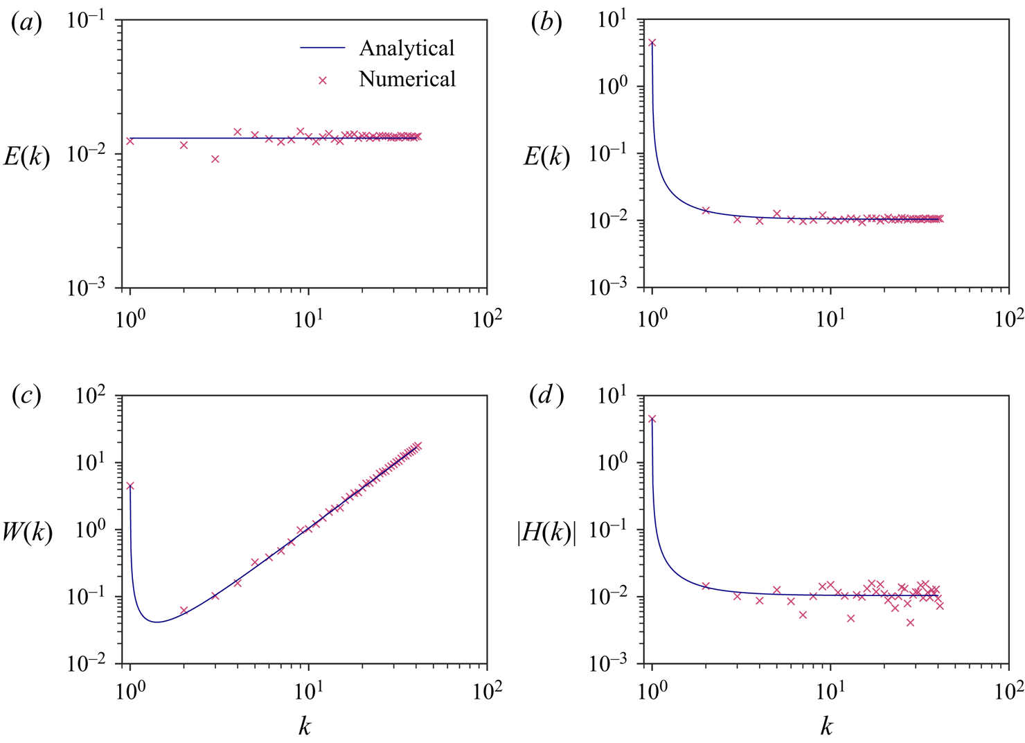
In figure 5, we compare the spectra associated with the relaxed state, obtained from the numerical simulations, with the predictions ((3.27a,b) and (3.28)) for the spectra. An excellent agreement is observed. Figure 5(a) shows the mirror-symmetric case, where a flat energy spectrum, associated with equidistributed enstrophy is obtained. We do not show the enstrophy spectrum, which is simply obtained by the energy spectrum multiplied by $k^2$.

Figure 5.

Analytical spectra associated with the absolute equilibrium state and numerical spectra. (a) Energy spectrum of the helicity-free case at $t=140$. (b–d) Helical case at $t=30$. (b) Energy spectrum. (c) Enstrophy spectrum. (d) Absolute value of helicity spectrum.

The most flagrant difference between the mirror-symmetric and helical cases is the accumulation of helicity near the infrared cut-off. In figure 5(b), we observe this for the energy spectrum, and the same feature is observed for the enstrophy and helicity spectra in figures 5(c) and figure 5(d), respectively. The amount of energy in this large-scale feature is quite important. Indeed, the $k=1$ mode contains $87\,\%$ of the total energy. We will now focus on this energetic, helical mode.

5.3. Visualization of the final state

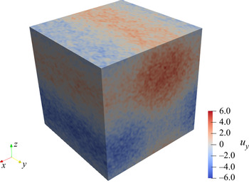
An instantaneous visualization of the $y$-component of the velocity for the final state is visualized in figure 6. It shows that our 3-D, inviscid, no vortex-stretching system relaxes to a large-scale structure. This could be suspected from the energy spectrum, and it is illustrated in the visualizations. Because almost all energy and all helicity is contained in the $k=1$ mode, a plausible 3-D structure is the Arnold–Beltrami–Childress, or ABC, flow. A physical explanation for this, in the light of the statistical mechanics description used here, is that adding the additional constraint of helicity conservation will change the energy and therefore the enstrophy distribution. This will necessarily lead to a decrease of the entropy of the system, because the highest entropy corresponds to enstrophy equipartition. The minimum change in entropy corresponds to a modification of the largest scales of the system. Maximizing the helicity in the largest scales of the system is therefore the most probable reaction of the system. Maximum helicity corresponds to alignment of velocity and vorticity, and thus to an ABC flow. In the following, we verify that the $k=1$ contribution of the equilibrium state corresponds to such a flow.

Figure 6.

Visualizations of the truncated inviscid system without vortex stretching, obtained from pseudo-spectral computations. Velocity in the $y$-direction ($u_y$).

The definition of an ABC flow with typical size $L$ is

(5.1)\begin{equation} \left. \begin{gathered} u_x= A \sin \tilde z+C \cos \tilde y, \\ u_y=B \sin \tilde x+A \cos \tilde z,\\ u_z=C \sin \tilde y+B \cos \tilde x, \end{gathered} \right\} \end{equation}

where $\tilde x_i=\pm 2{\rm \pi} x_i/L + \phi _{i}$. The $\pm$ sign determines the sign of helicity. Simple algebra shows that the parameters $A,B,C$ satisfy the relations

(5.2)\begin{equation} \left. \begin{gathered} A^2= \left\langle u_{x}^2 \right\rangle +\left\langle u_{y}^2\right\rangle -\left\langle u_{z}^2\right\rangle , \\ B^2=\left\langle u_{y}^2\right\rangle +\left\langle u_{z}^2\right\rangle -\left\langle u_{x}^2\right\rangle , \\ C^2= \left\langle u_{z}^2\right\rangle +\left\langle u_{x}^2\right\rangle -\left\langle u_{y}^2\right\rangle . \end{gathered} \right\} \end{equation}

We measure during equilibrium $\left \langle u_{x}^2 \right \rangle =3.7963$, $\left \langle u_{y}^2 \right \rangle =4.2210$ and $\left \langle u_{z}^2 \right \rangle =1.8600$. These figures yield $|A|=2.4814$, $|B|=1.5115$ and $|C|=1.1980$. Averaging the three relations (5.1) for fixed positions $x,y,z$ allows us also to determine the phases $\phi _{i}$. Doing so for our simulation, we find $\tilde {x}=-2{\rm \pi} x/L-0.66{\rm \pi}, \tilde {y}=-2{\rm \pi} y/L-0.25{\rm \pi}, \tilde {z}=-2{\rm \pi} z/L-0.495{\rm \pi}$ with $A>0$, $B>0$, $C>0$.

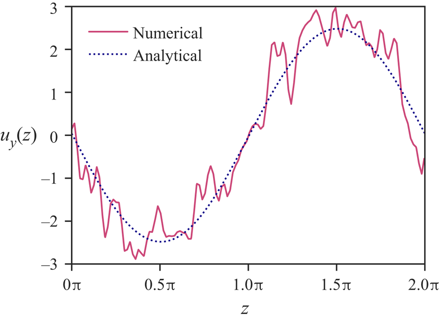
In figure 7, we compare the resulting ABC flow prediction to the results of the simulation for an arbitrary cut through the domain along the $z$-direction, plotting the $y$-velocity. The large-scale flow is indeed consistent with an ABC flow pattern. Superposed upon this large-scale pattern, we observe random fluctuations with a larger spatial frequency, consistent with the spectra we showed in the previous section. All other velocity components in all other directions (not shown) confirm this behaviour of an ABC structure accompanied by large-frequency noise.

Figure 7.

Visualization of flow and verification of ABC flow proprieties. Analytical and numerical results of $u_y(z)$ along the line ($x=0.66L$, $y=0.5L$).