1 Introduction
The interactions between wind and water waves influence the sea states, marine atmospheric boundary layer and upper-ocean dynamics. Strong wind forcing leads to wave breaking in oceans, which plays an important role in air–sea interactions. As summarized in many review papers (see for example, Banner & Peregrine Reference Banner and Peregrine1993; Melville Reference Melville1996; Perlin & Schultz Reference Perlin and Schultz2000; Duncan Reference Duncan2001; Kiger & Duncan Reference Kiger and Duncan2012; Perlin, Choi & Tian Reference Perlin, Choi and Tian2013), wave breaking limits the amplitude of surface waves, generates ocean currents, vorticity and turbulence and enhances the transport of mass, momentum and energy between the atmosphere and oceans. The investigation of wind over breaking waves is helpful for the development of ocean–atmosphere interaction models.
Extensive field measurements, laboratory experiments and numerical simulations have been conducted to study breaking waves. The previous studies covered various aspects of the flow physics, including the instability mechanisms leading to wave breaking (e.g. McLean et al. Reference McLean, Ma, Martin, Saffman and Yuen1982; Melville Reference Melville1982; Su et al. Reference Su, Bergin, Marler and Myrick1982; Longuet-Higgins & Tanaka Reference Longuet-Higgins and Tanaka1997a ,Reference Longuet-Higgins and Tanaka b ), geometrical properties of breaking waves (e.g. Duncan Reference Duncan1981, Reference Duncan1983; Longuet-Higgins Reference Longuet-Higgins1982; New Reference New1983; Bonmarin Reference Bonmarin1989; Skyner Reference Skyner1996; Chang & Liu Reference Chang and Liu1998; Duncan et al. Reference Duncan, Qiao, Philomin and Wenz1999; Melville, Veron & White Reference Melville, Veron and White2002; Wu & Yao Reference Wu and Yao2004; Diorio, Liu & Duncan Reference Diorio, Liu and Duncan2009; Babanin et al. Reference Babanin, Chalikov, Young and Savelyev2010), onset criteria for wave breaking (e.g. Duncan Reference Duncan1983; Bonmarin & Ramamonjiarisoa Reference Bonmarin and Ramamonjiarisoa1985; Rapp & Melville Reference Rapp and Melville1990; Schultz, Huh & Griffin Reference Schultz, Huh and Griffin1994; Perlin, He & Bernal Reference Perlin, He and Bernal1996; Banner & Tian Reference Banner and Tian1998; Johannessen & Swan Reference Johannessen and Swan2001; Qiao & Duncan Reference Qiao and Duncan2001; Song & Banner Reference Song and Banner2002; Stansell & MacFarlane Reference Stansell and MacFarlane2002; Wu & Nepf Reference Wu and Nepf2002; Yao & Wu Reference Yao and Wu2005; Babanin et al. Reference Babanin, Chalikov, Young and Savelyev2007; Chiang & Hwung Reference Chiang and Hwung2007; Kharif et al. Reference Kharif, Giovanangeli, Touboul, Grare and Pelinovsky2008; Tian, Perlin & Choi Reference Tian, Perlin and Choi2008; Toffoli et al. Reference Toffoli, Babanin, Onorato and Waseda2010), mechanisms of air entrainment (e.g. Lamarre & Melville Reference Lamarre and Melville1991; Deane & Stokes Reference Deane and Stokes2002; Blenkinsopp & Chaplin Reference Blenkinsopp and Chaplin2007; Wang, Yang & Stern Reference Wang, Yang and Stern2016), capillary effects (e.g. Longuet-Higgins Reference Longuet-Higgins1992; Perlin, Lin & Ting Reference Perlin, Lin and Ting1993; Zhang Reference Zhang1995; Fedorov, Melville & Rozenberg Reference Fedorov, Melville and Rozenberg1998; Jiang et al. Reference Jiang, Lin, Schultz and Perlin1999; Deike, Popinet & Melville Reference Deike, Popinet and Melville2015) and transport of momentum and energy (e.g. Rapp & Melville Reference Rapp and Melville1990; Nepf, Wu & Chan Reference Nepf, Wu and Chan1998; Tulin & Waseda Reference Tulin and Waseda1999; Meza, Zhang & Seymour Reference Meza, Zhang and Seymour2000; Yao & Wu Reference Yao and Wu2004; Banner & Peirson Reference Banner and Peirson2007; Drazen, Melville & Lenain Reference Drazen, Melville and Lenain2008; Iafrati Reference Iafrati2009; Tian, Perlin & Choi Reference Tian, Perlin and Choi2010; Babanin Reference Babanin2011).
Many laboratory experiments have been conducted to study the wind field over breaking waves. Banner & Melville (Reference Banner and Melville1976) discovered that the onset of wave breaking is accompanied by airflow separation. Their analysis was based on steady wave breakers, which are nearly stationary in the coordinate fixed to the waves. Kawai (Reference Kawai1982) and Kawamura & Toba (Reference Kawamura and Toba1988) investigated wind over unsteady breaking waves. They observed airflow separation from the wave crest. Reul, Branger & Giovanangeli (Reference Reul, Branger and Giovanangeli1999) further measured the flow field in the region extending to the vicinity of the air–water interface. They found that the geometry of the breaking front resembles a backward-facing step, and crest-to-crest airflow separation takes place over a chain of breaking waves. Although airflow separation can also take place over non-breaking waves (Weissman Reference Weissman, Phillips and Hasselmann1986), Reul, Branger & Giovanangeli (Reference Reul, Branger and Giovanangeli2008) pointed out that the separation induced by breaking waves is stronger and more consistent. Buckley & Veron (Reference Buckley and Veron2016) studied wind over waves with a range of wave ages, defined as the ratio of the wave phase speed to the characteristic velocity of wind. They reported that the airflow separation happens at small wave ages but is absent at large wave ages.
The airflow separation influences the transport of momentum between air and water. Banner & Melville (Reference Banner and Melville1976) showed that the drag force exerted on the wind is significantly larger over breaking waves than over non-breaking waves. Banner (Reference Banner1990) attributed the high drag of wind over breaking waves to the pressure minimum and maximum occurring on the leeward and windward of the wave crest, respectively. Banner & Peirson (Reference Banner and Peirson1998) and Belcher & Hunt (Reference Belcher and Hunt1998) pointed out that the significant increase of the pressure drag with the wave steepness is responsible for the high total drag of wind over breaking waves. By assuming that the wave surface forms a backward-facing step during wave breaking, Kudryavtsev & Makin (Reference Kudryavtsev and Makin2001) proposed a wind–wave coupled model to account for the form drag augment related to wave breaking.
It was discovered in many field measurements (Powell, Vickery & Reinhold Reference Powell, Vickery and Reinhold2003; Jarosz et al. Reference Jarosz, Mitchell, Wang and Teague2007; Bell, Montgomery & Emanuel Reference Bell, Montgomery and Emanuel2012; Holthuijsen, Powell & Pietrzak Reference Holthuijsen, Powell and Pietrzak2012; Zhao et al. Reference Zhao, Liu, Li, Dai, Song and Lv2015), laboratory experiments (Donelan et al. Reference Donelan, Haus, Reul, Plant, Stiassnie, Graber, Brown and Saltzman2004; Takagaki et al. Reference Takagaki, Komori, Suzuki, Iwano, Kuramoto, Shimada, Kurose and Takahashi2012; Troitskaya et al. Reference Troitskaya, Sergeev, Kandaurov, Baidakov, Vdovin and Kazakov2012), and numerical simulations based on wind–wave coupled models (Moon, Ginis & Hara Reference Moon, Ginis and Hara2004; Kudryavtsev & Makin Reference Kudryavtsev and Makin2007; Mueller & Veron Reference Mueller and Veron2009; Liu, Guan & Xie Reference Liu, Guan and Xie2012) that the drag coefficient saturates at high wind speeds. New interests were then drawn to the research of wind during wave breaking, wherein the airflow separation over the wave crest is regarded as one of the possible physical processes leading to the saturation of the drag coefficient. Veron, Saxena & Misra (Reference Veron, Saxena and Misra2007) measured the flow field inside the viscous sublayer over wind-generated breaking waves to study the along-surface viscous shear stress. They observed that due to the airflow separation, there is a drastic drop of the surface tangential stress near the wave trough. Reul et al. (Reference Reul, Branger and Giovanangeli2008) conducted experiments to study the airflow separation over mechanically generated breaking waves. They showed that the separation layer becomes higher as the wave steepness increases, and the surface tangential stress is low inside the separation bubble.
To date, most understandings of the physics of wind over breaking waves have come from laboratory experiments and field measurements. As an important complementary research tool to experiments, numerical simulations are able to provide details of the flow field. Although numerical simulations have been used to study wave breaking (Chen et al. Reference Chen, Kharif, Zaleski and Li1999; Song & Sirviente Reference Song and Sirviente2004; Iafrati Reference Iafrati2009, Reference Iafrati2011; Tian, Perlin & Choi Reference Tian, Perlin and Choi2012; Iafrati, Babanin & Onorato Reference Iafrati, Babanin and Onorato2013; Derakhti & Kirby Reference Derakhti and Kirby2014; Deike et al. Reference Deike, Popinet and Melville2015; Lubin & Glockner Reference Lubin and Glockner2015; Deike, Melville & Popinet Reference Deike, Melville and Popinet2016; Derakhti & Kirby Reference Derakhti and Kirby2016; Pizzo, Deike & Melville Reference Pizzo, Deike and Melville2016), much less attention was paid to the wind turbulence over breaking waves.
The numerical methods for simulating flows with a wave surface can be categorized into one-fluid and two-fluid simulations. The one-fluid simulation has been successfully used to study airflow over prescribed non-breaking waves (see e.g. Sullivan, McWilliams & Moeng Reference Sullivan, McWilliams and Moeng2000; Yang & Shen Reference Yang and Shen2010; Druzhinin, Troitskaya & Zilitinkevich Reference Druzhinin, Troitskaya and Zilitinkevich2012; Sullivan, McWilliams & Patton Reference Sullivan, McWilliams and Patton2014; Hara & Sullivan Reference Hara and Sullivan2015). To study the effect of wave breaking on wind turbulence using one-fluid simulations, Suzuki, Hara & Sullivan (Reference Suzuki, Hara and Sullivan2015) modelled the impact of wave breaking events by adding localized form drag. Sullivan et al. (Reference Sullivan, Banner, Morison and Peirson2018) extended the application of one-fluid simulations to the investigation of wind over steady breaking waves and unsteady steep waves, wherein the waves act as a bottom boundary with prescribed motions obtained from potential flow theory or measurements. In two-fluid simulations, the air and water are treated as a coherent system. The two-fluid simulation needs an interface-capturing technique, which includes but is not limited to the level-set (LS) method (e.g. Osher & Sethian Reference Osher and Sethian1988; Sussman, Smereka & Osher Reference Sussman, Smereka and Osher1994; Sussman et al. Reference Sussman, Fatemi, Smereka and Osher1998), volume-of-fluid (VOF) method (e.g. Scardovelli & Zaleski Reference Scardovelli and Zaleski1999; López et al. Reference López, Hernández, Gómez and Faura2005; Weymouth & Yue Reference Weymouth and Yue2010) and coupled LS and VOF (CLSVOF) method (e.g. Sussman & Puckett Reference Sussman and Puckett2000; Liu Reference Liu2012). In general, the VOF method has good performance in conserving the mass of each phase of the fluids, while the LS method can capture the geometry of waves accurately.
Although the numerical method for the two-fluid simulation is relatively mature, it is challenging to conduct fine-resolution simulations of breaking waves due to the high computational cost. Previously, two-dimensional (2-D) simulations were performed to describe the general process of wave breaking (Chen et al. Reference Chen, Kharif, Zaleski and Li1999; Song & Sirviente Reference Song and Sirviente2004), study the energy dissipation (Chen et al. Reference Chen, Kharif, Zaleski and Li1999; Iafrati Reference Iafrati2009, Reference Iafrati2011), investigate the effects of surface tension (Song & Sirviente Reference Song and Sirviente2004; Deike et al. Reference Deike, Popinet and Melville2015) and wave steepness (Iafrati Reference Iafrati2009; Deike et al. Reference Deike, Popinet and Melville2015) and analyse the influence of wave breaking on the initially stationary air (Iafrati et al. Reference Iafrati, Babanin and Onorato2013). However, 2-D simulations cannot capture turbulence without using turbulent models. In this sense, three-dimensional (3-D) simulations are desired to study the dynamics of wind turbulence over breaking waves.
In the present study, we perform direct numerical simulations (DNS) of turbulent wind over breaking waves with the breaking process explicitly resolved. The air–water interfaces are captured using the CLSVOF method. The objective is to study the effect of wave breaking on the momentum and energy transfer in the airflow. The effects of wave age and wave steepness are analysed. The remainder of this paper is organized as follows: in § 2, the numerical algorithms are introduced; in § 3, the simulation parameters are described; in § 4, the results are analysed, including mean velocity, cross-surface momentum flux, Reynolds stress and turbulence kinetic energy; in § 5, major conclusions are summarized.
2 Governing equations and numerical algorithms
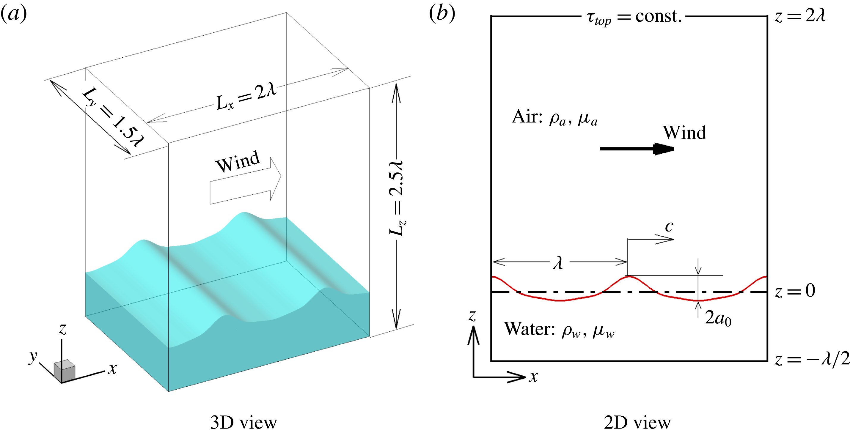
Computational domain and coordinate system for DNS of wind over steep and breaking waves.

Figure 1 shows the computational domain and coordinates used in the present simulations. Let
 $x$
,
 $y$
and
 $z$
(or
 $x_{1}$
,
 $x_{2}$
and
 $x_{3}$
) denote respectively the streamwise, spanwise and vertical directions, with the corresponding velocity components represented by
 $u$
,
 $v$
and
 $w$
(or
 $u_{1}$
,
 $u_{2}$
and
 $u_{3}$
), respectively. The air and water are treated as a coherent system with the density and viscosity varying with the fluid phase. The flows of air and water are governed by the following continuity and momentum equations:
 $$\begin{eqnarray}\displaystyle & \displaystyle \frac{\unicode[STIX]{x2202}u_{i}}{\unicode[STIX]{x2202}x_{i}}=0, & \displaystyle\end{eqnarray}$$
 $$\begin{eqnarray}\displaystyle & \displaystyle \unicode[STIX]{x1D70C}(\unicode[STIX]{x1D719})\left(\frac{\unicode[STIX]{x2202}u_{i}}{\unicode[STIX]{x2202}t}+u_{j}\frac{\unicode[STIX]{x2202}u_{i}}{\unicode[STIX]{x2202}x_{j}}\right)=-\frac{\unicode[STIX]{x2202}p}{\unicode[STIX]{x2202}x_{i}}+\frac{\unicode[STIX]{x2202}(2\unicode[STIX]{x1D707}(\unicode[STIX]{x1D719})\unicode[STIX]{x1D61A}_{ij})}{\unicode[STIX]{x2202}x_{j}}-\unicode[STIX]{x1D70C}(\unicode[STIX]{x1D719})g\unicode[STIX]{x1D6FF}_{i3}+\unicode[STIX]{x1D6FE}\unicode[STIX]{x1D705}\unicode[STIX]{x1D6FF}_{s}(\unicode[STIX]{x1D719})n_{i}. & \displaystyle\end{eqnarray}$$
Here,
 $t$
is the time;
 $\unicode[STIX]{x1D70C}$
and
 $\unicode[STIX]{x1D707}$
are respectively the density and dynamic viscosity of the fluid;
 $\unicode[STIX]{x1D719}$
is the LS function, defined as the signed distance from the air–water interface with its value being positive and negative in water and air, respectively;
 $p$
is the pressure;
 $\unicode[STIX]{x1D61A}_{ij}=(\unicode[STIX]{x2202}u_{i}/\unicode[STIX]{x2202}x_{j}+\unicode[STIX]{x2202}u_{j}/\unicode[STIX]{x2202}x_{i})/2$
is the strain rate tensor;
 $g$
is the gravitational acceleration;
 $\unicode[STIX]{x1D6FF}_{ij}$
is the Kronecker delta tensor;
 $\unicode[STIX]{x1D6FE}$
is the surface tension;
 $\unicode[STIX]{x1D705}=\unicode[STIX]{x1D735}\boldsymbol{\cdot }(\unicode[STIX]{x1D735}\unicode[STIX]{x1D719})$
at
 $\unicode[STIX]{x1D719}=0$
is the curvature of the air–water interface;
 $\unicode[STIX]{x1D6FF}_{s}(\unicode[STIX]{x1D719})$
is the Dirac delta function at the interface; and
 $\boldsymbol{n}=[n_{1},n_{2},n_{3}]^{\text{T}}=\unicode[STIX]{x1D735}\unicode[STIX]{x1D719}$
at
 $\unicode[STIX]{x1D719}=0$
is the normal direction of the interface, orientating from water towards air. Periodic boundary conditions are imposed in
 $x$
- and
 $y$
-directions. No-slip boundary condition is applied at the bottom of water. At the top of air, the wind is driven by a constant shear stress
 $\unicode[STIX]{x1D70F}_{top}$
in the streamwise direction, while shear-free (
 $\unicode[STIX]{x2202}v/\unicode[STIX]{x2202}z=0$
) and impenetrable (
 $w=0$
) conditions are prescribed for velocity components in
 $y$
- and
 $z$
-directions, respectively.
The computational domain size is set to
 $L_{x}\times L_{y}\times L_{z}=2\unicode[STIX]{x1D706}\times 1.5\unicode[STIX]{x1D706}\times 2.5\unicode[STIX]{x1D706}$
, where
 $\unicode[STIX]{x1D706}$
is the wavelength of the primary wave studied (figure 1). The mean elevation of water is set to
 $z=0$
. The mean water depth
 $d$
and air height
 $h$
are
 $0.5\unicode[STIX]{x1D706}$
and
 $2\unicode[STIX]{x1D706}$
, respectively. The dispersion parameter
 $kd$
is
 $\unicode[STIX]{x03C0}$
, satisfying the deep water wave condition (Mei Reference Mei1983), where
 $k=2\unicode[STIX]{x03C0}/\unicode[STIX]{x1D706}$
is the wavenumber. The number of grid points used in the simulations is
 $N_{x}\times N_{y}\times N_{z}=320\times 192\times 360$
. In the
 $x$
- and
 $y$
-directions, the grid is evenly spaced. In the
 $z$
-direction, the grid is clustered between
 $z=-0.1\unicode[STIX]{x1D706}$
and
 $z=0.15\unicode[STIX]{x1D706}$
with a fine and constant resolution of
 $\unicode[STIX]{x1D6E5}_{z}=0.002\unicode[STIX]{x1D706}$
, and the grid is stretched to the top of air and bottom of water. There are 286 and 74 grid points used for
 $z>0$
and
 $z<0$
, respectively.
Equation (2.2) is spatially discretized using the second-order central difference scheme. The second-order Runge–Kutta (RK2) method is utilized for the time integration. At each sub-step of the RK2 method, the fractional-step method (Kim & Moin Reference Kim and Moin1985) is used to enforce the divergence-free condition (2.1). The pressure is governed by the following Poisson equation (Yang et al. Reference Yang, Lu, Guo, Liu and Shen2017)
 $$\begin{eqnarray}\displaystyle \frac{\unicode[STIX]{x2202}}{\unicode[STIX]{x2202}x_{i}}\left(\frac{1}{\unicode[STIX]{x1D70C}}\frac{\unicode[STIX]{x2202}p}{\unicode[STIX]{x2202}x_{i}}\right)=\frac{1}{\unicode[STIX]{x1D6FC}\unicode[STIX]{x0394}t}\frac{\unicode[STIX]{x2202}u_{i}^{t}}{\unicode[STIX]{x2202}x_{i}}, & & \displaystyle\end{eqnarray}$$
where
 $\unicode[STIX]{x1D6FC}$
is a coefficient corresponding to the RK2 method, of which the value is 1.0 and 0.5 in the first and second sub-steps, respectively,
 $\unicode[STIX]{x0394}t$
is the time step and
 $u_{i}^{t}$
is the temporal velocity without considering the effect of the pressure term in (2.2). Equation (2.3) is solved using the Portable, Extensible Toolkit for Scientific Computation (PETSc) math library (Balay et al.
Reference Balay, Gropp, McInnes, Smith, Arge, Bruaset and Langtangen1997).
The air–water interfaces are tracked using the CLSVOF method. The LS method solves the following advection equation of the LS function
 $$\begin{eqnarray}\displaystyle \frac{\unicode[STIX]{x2202}\unicode[STIX]{x1D719}}{\unicode[STIX]{x2202}t}+u_{j}\frac{\unicode[STIX]{x2202}\unicode[STIX]{x1D719}}{\unicode[STIX]{x2202}x_{j}}=0. & & \displaystyle\end{eqnarray}$$
This equation is spatially discretized using the second-order essential non-oscillatory scheme (Shu & Osher Reference Shu and Osher1989), and the second-order operator-splitting method (Sussman & Puckett Reference Sussman and Puckett2000) is applied for the time integration. The reinitialization procedure of Sussman et al. (Reference Sussman, Smereka and Osher1994) is applied after solving (2.4) at every time step, such that
 $\unicode[STIX]{x1D719}$
maintains the property of a distance function
 $|\unicode[STIX]{x1D735}\unicode[STIX]{x1D719}|=1$
.
The LS function is coupled to the momentum (2.2) through the density and viscosity as
 $$\begin{eqnarray}\displaystyle & \displaystyle \unicode[STIX]{x1D70C}=H(\unicode[STIX]{x1D719},\unicode[STIX]{x1D6E5}_{s})\unicode[STIX]{x1D70C}_{w}+[1-H(\unicode[STIX]{x1D719},\unicode[STIX]{x1D6E5}_{s})]\unicode[STIX]{x1D70C}_{a}, & \displaystyle\end{eqnarray}$$
 $$\begin{eqnarray}\displaystyle & \displaystyle \unicode[STIX]{x1D707}=H(\unicode[STIX]{x1D719},\unicode[STIX]{x1D6E5}_{s})\unicode[STIX]{x1D707}_{w}+[1-H(\unicode[STIX]{x1D719},\unicode[STIX]{x1D6E5}_{s})]\unicode[STIX]{x1D707}_{a}, & \displaystyle\end{eqnarray}$$
where the subscripts ‘
 $a$
’ and ‘
 $w$
’ represent air and water, respectively. The smoothed Heaviside function
 $H(\unicode[STIX]{x1D719},\unicode[STIX]{x1D6E5}_{s})$
reads
 $$\begin{eqnarray}\displaystyle H(\unicode[STIX]{x1D719},\unicode[STIX]{x1D6E5}_{s})=\left\{\begin{array}{@{}ll@{}}0\quad & \unicode[STIX]{x1D719}<-\unicode[STIX]{x1D6E5}_{s},\\ \displaystyle \frac{1}{2}\left[1+\frac{\unicode[STIX]{x1D719}}{\unicode[STIX]{x1D6E5}_{s}}+\frac{1}{\unicode[STIX]{x03C0}}\sin \left(\frac{\unicode[STIX]{x1D719}\unicode[STIX]{x03C0}}{\unicode[STIX]{x1D6E5}_{s}}\right)\right]\quad & |\unicode[STIX]{x1D719}|\leqslant \unicode[STIX]{x1D6E5}_{s},\\ 1\quad & \unicode[STIX]{x1D719}>\unicode[STIX]{x1D6E5}_{s}.\end{array}\right. & & \displaystyle\end{eqnarray}$$
Here,
 $\unicode[STIX]{x1D6E5}_{s}$
is set to three times the vertical grid size.
The mass conservation for each phase of fluid is enforced using the VOF method, which solves the following convection equation of the VOF function
 $$\begin{eqnarray}\displaystyle \frac{\unicode[STIX]{x2202}\unicode[STIX]{x1D713}}{\unicode[STIX]{x2202}t}+\frac{\unicode[STIX]{x2202}(u_{j}\unicode[STIX]{x1D713})}{\unicode[STIX]{x2202}x_{j}}=0. & & \displaystyle\end{eqnarray}$$
Here,
 $\unicode[STIX]{x1D713}$
is defined as the volume fraction of water in a computational cell, from which it is known that
 $\unicode[STIX]{x1D713}=0$
in the air,
 $\unicode[STIX]{x1D713}=1$
in the water and
 $0<\unicode[STIX]{x1D713}<1$
in cells containing the air–water interface. The conservative VOF method (Weymouth & Yue Reference Weymouth and Yue2010) is implemented to solve (2.8). The CLSVOF method of Sussman & Puckett (Reference Sussman and Puckett2000) is employed to couple
 $\unicode[STIX]{x1D719}$
and
 $\unicode[STIX]{x1D713}$
, wherein the flux of
 $\unicode[STIX]{x1D713}$
is calculated based on the interface reconstructed using the piecewise linear interface calculation (PLIC) algorithm with the help of
 $\unicode[STIX]{x1D719}$
, and the value of
 $\unicode[STIX]{x1D719}$
near the interface is determined using
 $\unicode[STIX]{x1D713}$
. More detailed descriptions of the numerical method and validations are given in Liu (Reference Liu2012) and Yang et al. (Reference Yang, Lu, Guo, Liu and Shen2017).
3 Simulation cases
3.1 Initialization of flow field
The initial condition in the simulations is fully developed wind turbulence over strongly forced steep waves. Following the practice of many previous two-fluid numerical simulations of wave breaking (Chen et al. Reference Chen, Kharif, Zaleski and Li1999; Iafrati Reference Iafrati2009; Tian et al. Reference Tian, Perlin and Choi2010; Hu et al. Reference Hu, Guo, Lu, Liu, Dalrymple and Shen2012; Deike et al. Reference Deike, Popinet and Melville2015; Lubin & Glockner Reference Lubin and Glockner2015; Deike et al. Reference Deike, Melville and Popinet2016), the initial water elevation is given as the analytical solution of Stokes wave at the third-order perturbation expansion of the wave steepness (Lamb Reference Lamb1932), viz.
 $$\begin{eqnarray}\displaystyle \unicode[STIX]{x1D702}(x)=a_{0}\cos (kx-\unicode[STIX]{x1D714}t)+{\textstyle \frac{1}{2}}\unicode[STIX]{x1D700}_{0}a_{0}\cos [2(kx-\unicode[STIX]{x1D714}t)]+{\textstyle \frac{3}{8}}\unicode[STIX]{x1D700}_{0}^{2}a_{0}\cos [3(kx-\unicode[STIX]{x1D714}t)], & & \displaystyle\end{eqnarray}$$
where
 $\unicode[STIX]{x1D702}$
is the surface elevation;
 $a_{0}$
is the initial amplitude of the linear wave component (the first term on the right-hand side of (3.1));
 $\unicode[STIX]{x1D700}_{0}=ka_{0}$
is the initial linear wave steepness; and
 $\unicode[STIX]{x1D714}=\sqrt{gk(1+\unicode[STIX]{x1D700}_{0}^{2})}$
is the angular frequency. The velocity in water is given correspondingly based on the potential flow theory (Lamb Reference Lamb1932). Equation (3.1) is used to prescribe the wave geometry, while the airflow is simulated based on the prescribed top shear stress and wave surface kinematics. Once the wind turbulence field is fully developed, the two-fluid flow field is output at different time as the initial condition for the different runs of the simulation of wind over breaking waves, such that the initial turbulence fluctuations vary among different runs. The air and water evolve dynamically from then on.
3.2 Computational parameters
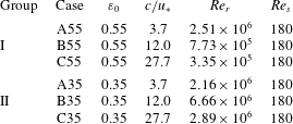
Specified computational parameters for airflow over breaking waves.
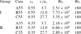
Table 1 summarizes the key parameters of the simulation cases. Six cases have been considered, which can be categorized into two groups. Group I consists of cases A55, B55 and C55, in which
 $\unicode[STIX]{x1D700}_{0}=0.55$
and plunging breakers are generated. We remark that the use of a very steep wave is a computationally effective method of initializing plunging breakers in numerical simulation (e.g. Chen et al.
Reference Chen, Kharif, Zaleski and Li1999; Iafrati Reference Iafrati2009; Deike et al.
Reference Deike, Popinet and Melville2015; Lubin & Glockner Reference Lubin and Glockner2015; Yang et al.
Reference Yang, Lu, Guo, Liu and Shen2017). Generating plungers with the wave-focusing method (Derakhti & Kirby Reference Derakhti and Kirby2016) is more physical, but computationally more expensive especially with the incorporation of wind turbulence simulation. In future studies, with the increase of computer power, such approaches should be considered. The wave age
 $c/u_{\ast }$
in cases A55, B55 and C55 is 3.7 (young wave), 12.0 (intermediate wave) and 27.7 (old wave), respectively (Sullivan et al.
Reference Sullivan, McWilliams and Moeng2000; Yang & Shen Reference Yang and Shen2010). Here,
 $c=\unicode[STIX]{x1D714}/k$
characterizes the phase speed of the initial prescribed wave, and
 $u_{\ast }=\sqrt{\unicode[STIX]{x1D70F}_{top}/\unicode[STIX]{x1D70C}_{a}}$
is the frictional velocity in the air. Group II consists of cases A35, B35 and C35, in which
 $\unicode[STIX]{x1D700}_{0}=0.35$
and spilling breakers are generated. The waves ages in the group II cases are the same as those in the group I cases. If we consider waves with
 $\unicode[STIX]{x1D706}=20~\text{m}$
, the Reynolds number
 $Re_{r}=u_{\ast }\unicode[STIX]{x1D706}/\unicode[STIX]{x1D708}_{a}$
is
 $O(10^{5\sim 6})$
. We reduce the Reynolds number to
 $Re_{s}=180$
in the present study to perform DNS. Although large-eddy simulation (LES) is a possible tool for simulating wind turbulence over breaking waves at high Reynolds numbers, there are many challenges associated with LES. For example, the subgrid-scale modelling for air–water mixed flow and the wall-layer modelling near the complex wave surface with flow separation need substantial further studies, which are however, beyond the scope of this paper. In this study, we chose to use DNS because it has the advantage that the flow processes are directly captured, and no ad hoc turbulence modelling is needed. The reduction of the Reynolds number thickens the boundary layer of wind attached to the wave surface. Nevertheless, based on their numerical simulation results, Deike et al. (Reference Deike, Popinet and Melville2015) concluded that the Reynolds number does not play an important role in the breaking process. Instead, the wave steepness is the key parameter. Their conclusion was supported by previous laboratory experiments (Rapp & Melville Reference Rapp and Melville1990; Perlin et al.
Reference Perlin, Lin and Ting1993; Zhang Reference Zhang1995; Fedorov et al.
Reference Fedorov, Melville and Rozenberg1998; Duncan et al.
Reference Duncan, Qiao, Philomin and Wenz1999; Jiang et al.
Reference Jiang, Lin, Schultz and Perlin1999; Tulin & Waseda Reference Tulin and Waseda1999; Duncan Reference Duncan2001; Liu & Duncan Reference Liu and Duncan2003, Reference Liu and Duncan2006; Banner & Peirson Reference Banner and Peirson2007; Drazen et al.
Reference Drazen, Melville and Lenain2008; Caulliez Reference Caulliez2013, see also table 1 in Deike et al.
Reference Deike, Popinet and Melville2015).
3.3 Definition of turbulent statistics
Because the wave breaking of interest is highly unsteady and intermittent, time averaging cannot be used to define turbulent statistics in the present study of wind over breaking waves. Alternatively, we conduct many ensemble runs for each case starting with the same mean flow but with different initial fluctuations (§ 3.1), so that the ensemble over all runs can be used to calculate turbulence statistics. To be specific, in different runs of the same case, the initial wind profile and wave geometry are the same, but the instantaneous turbulence fluctuations are different. Once an initial field is obtained, the time of this field is set to
 $t=0$
for the simulation of wind over breaking waves. We run each sample till
 $t=3.0T$
, after which the wave breaking becomes less violent (see figure 4). Here,
 $T=2\unicode[STIX]{x03C0}/\unicode[STIX]{x1D714}$
is the period of the third-order Stokes waves based on the potential flow theory.
According to the above descriptions, it is understood that each field variable
 $f$
is a function of not only
 $x$
,
 $y$
,
 $z$
and
 $t$
, but also the sample index
 $n_{s}$
. We define ensemble averaging as
 $$\begin{eqnarray}\displaystyle \bar{f}(x_{i},z_{k},t)=\frac{1}{N_{w}N_{s}N_{y}}\mathop{\sum }_{n_{w}=0}^{N_{w}-1}\mathop{\sum }_{n_{s}=1}^{N_{s}}\mathop{\sum }_{j=1}^{N_{y}}f(x_{i}+n_{w}\unicode[STIX]{x1D706},y_{j},z_{k},t,n_{s}), & & \displaystyle\end{eqnarray}$$
where the overbar denotes an ensemble-averaged quantity. The subscripts
 $i$
,
 $j$
and
 $k$
are the indices of discretized grid points in the
 $x$
-,
 $y$
- and
 $z$
-directions, respectively;
 $N_{w}=2$
is the number of waves within the streamwise computational domain;
 $N_{s}=100$
is the total number of samples. The fluctuations with respect to the ensemble averaging are defined as
 $$\begin{eqnarray}\displaystyle \left.\begin{array}{@{}c@{}}\displaystyle f^{\prime \prime }(x,y,z,t,n_{s})=f(x,y,z,t,n_{s})-\bar{f}(x,z,t)\quad \text{for }0\leqslant x\leqslant \unicode[STIX]{x1D706},\\ \displaystyle f^{\prime \prime }(x,y,z,t,n_{s})=f(x,y,z,t,n_{s})-\bar{f}(x-\unicode[STIX]{x1D706},z,t)\quad \text{for }\unicode[STIX]{x1D706}\leqslant x\leqslant 2\unicode[STIX]{x1D706}.\end{array}\right\} & & \displaystyle\end{eqnarray}$$
Note that
 $f$
and
 $\bar{f}$
are defined in
 $[0,2\unicode[STIX]{x1D706}]$
and
 $[0,\unicode[STIX]{x1D706}]$
in the
 $x$
-direction, respectively. As a result, the definition of
 $f^{\prime \prime }$
is given separately in
 $[0,\unicode[STIX]{x1D706}]$
and
 $[\unicode[STIX]{x1D706},2\unicode[STIX]{x1D706}]$
in (3.3).
An ensemble-averaged quantity
 $\bar{f}$
can be further decomposed into a plane-averaged part
 $\langle f\rangle$
and a wave-coherent part
 $\tilde{f}$
as
 $$\begin{eqnarray}\displaystyle \bar{f}(x,z,t)=\langle f\rangle (z,t)+\tilde{f}(x,z,t), & & \displaystyle\end{eqnarray}$$
where the plane averaging is defined as
 $$\begin{eqnarray}\displaystyle \langle f\rangle (z,t)=\frac{N_{w}}{N_{x}}\mathop{\sum }_{i=1}^{N_{x}/N_{w}}\bar{f}(x_{i},z,t). & & \displaystyle\end{eqnarray}$$
The fluctuation
 $f^{\prime }(x,y,z,t,n_{s})$
with respect to the plane averaging is defined as
 $$\begin{eqnarray}\displaystyle f^{\prime }(x,y,z,t,n_{s})=f(x,y,z,t,n_{s})-\langle f\rangle (z,t). & & \displaystyle\end{eqnarray}$$
By substituting (3.4) into (3.3), a triple decomposition is obtained as
 $$\begin{eqnarray}\displaystyle f=\langle f\rangle +\tilde{f}+f^{\prime \prime }. & & \displaystyle\end{eqnarray}$$
Triple decomposition has been used to analyse the airflow over non-breaking waves (e.g. Hsu, Hsu & Street Reference Hsu, Hsu and Street1981; Sullivan et al.
Reference Sullivan, McWilliams and Moeng2000; Yang & Shen Reference Yang and Shen2010; Druzhinin et al. Reference Druzhinin, Troitskaya and Zilitinkevich2012). According to (3.6) and (3.7), the fluctuation with respect to the plane averaging
 $f^{\prime }$
can be decomposed into the fluctuation with respect to the ensemble-averaged part
 $f^{\prime \prime }$
and the wave-coherent part
 $\tilde{f}$
as
 $$\begin{eqnarray}\displaystyle f^{\prime }=\tilde{f}+f^{\prime \prime }. & & \displaystyle\end{eqnarray}$$
It can be proven from (3.2) that the ensemble averaging of the wave-coherent fluctuation is trivial, i.e.
 $$\begin{eqnarray}\displaystyle \bar{\tilde{f}}=0. & & \displaystyle\end{eqnarray}$$
Based on (3.8) and (3.9), it can be further derived that the total momentum flux
 $\overline{u_{i}^{\prime }u_{j}^{\prime }}$
can be decomposed into the contributions from
 $u_{i}^{\prime \prime }$
and
 $\tilde{u} _{i}$
as
 $$\begin{eqnarray}\displaystyle \overline{u_{i}^{\prime }u_{j}^{\prime }}=\overline{u_{i}^{\prime \prime }u_{j}^{\prime \prime }}+\overline{\tilde{u} _{i}\tilde{u} }_{j}. & & \displaystyle\end{eqnarray}$$
By applying (3.5), it is known that a similar decomposition holds for the total momentum flux with respect to the plane averaging as
 $$\begin{eqnarray}\displaystyle \langle u_{i}^{\prime }u_{j}^{\prime }\rangle =\langle u_{i}^{\prime \prime }u_{j}^{\prime \prime }\rangle +\langle \tilde{u} _{i}\tilde{u} _{j}\rangle . & & \displaystyle\end{eqnarray}$$
We note here that we have tested the effects of
 $N_{w}$
and
 $N_{s}$
on the simulation results of turbulence statistics. We have run case A55 using a larger computational domain with
 $L_{x}=4\unicode[STIX]{x1D706}$
and
 $N_{w}=4$
. We found that the results demonstrated in this paper are not altered. We have also performed a sample-number convergence test for case A55. The results obtain from
 $N_{s}=50$
, 100 and 200 are compared with each other. We found that increasing the number of samples results in a negligibly small change of turbulence statistics. For example, the plane-averaged streamwise velocity
 $\langle u\rangle$
for the three
 $N_{s}$
varies less than
 $1\,\%$
. The difference in the total momentum flux
 $\langle u^{\prime }w^{\prime }\rangle$
is less than
 $4\,\%$
between
 $N_{s}=50$
and 100, and is less than
 $2\,\%$
between
 $N_{s}=100$
and 200.
4 Results
4.1 Validation
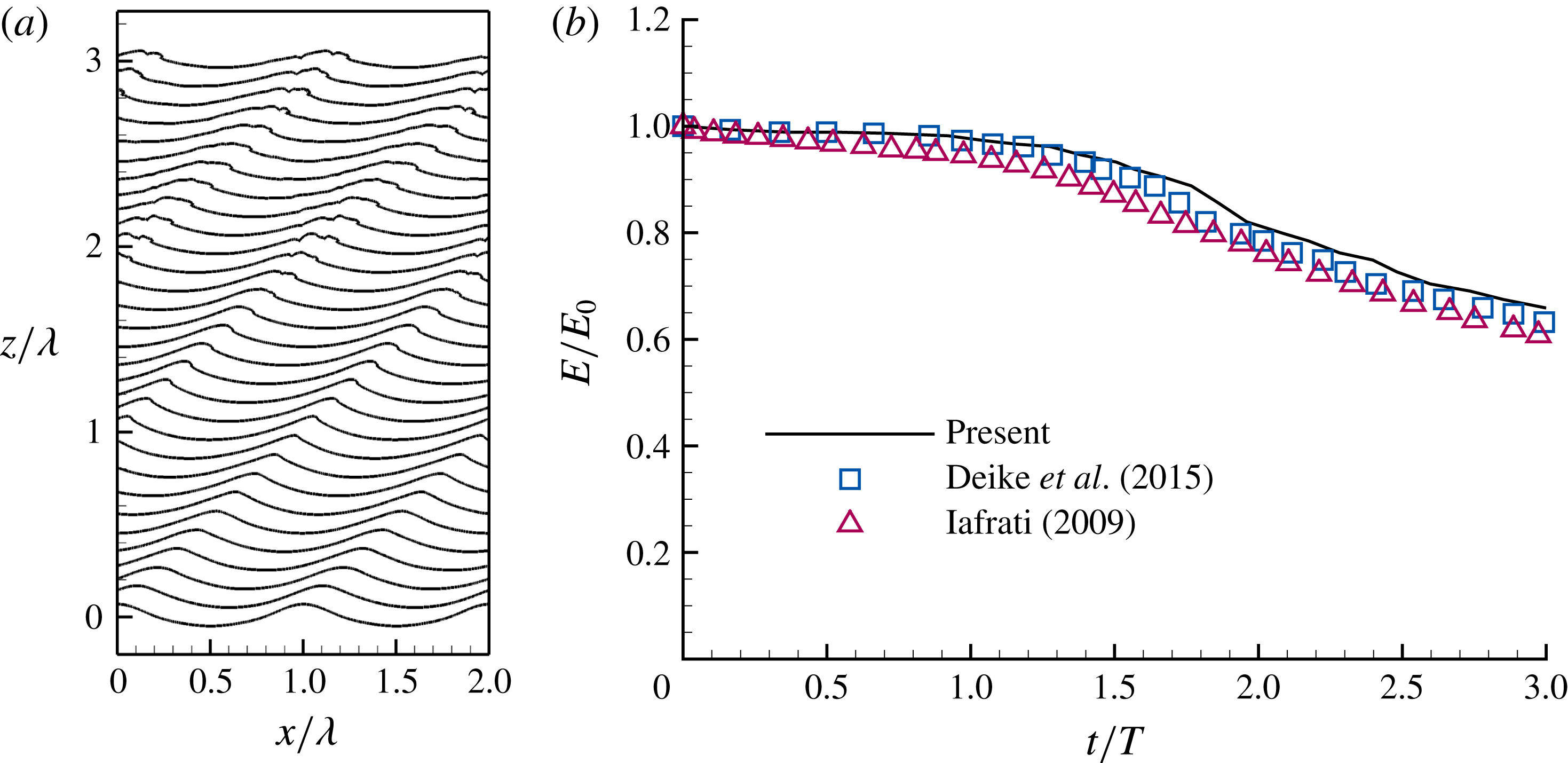
Simulation results for wave breaking with
 $\unicode[STIX]{x1D716}=0.35$
and
 $u_{\ast }=0$
. (a) Wave geometry from
 $t=0$
to
 $3.0T$
. The wave surface is shifted by
 $ct/\unicode[STIX]{x1D706}$
in the
 $+z$
-direction. (b) Time series of total energy
 $E$
.
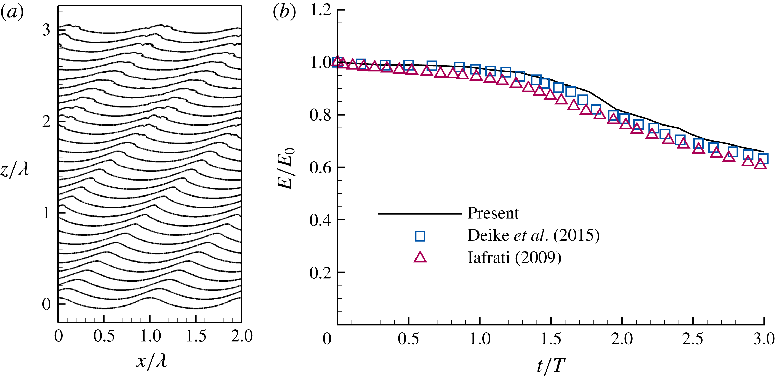
Figure 2(a) shows the surfaces of breaking waves with
 $\unicode[STIX]{x1D716}=0.35$
without wind, from
 $t=0$
to
 $3.0T$
. The wave surface at
 $t$
is shifted by
 $ct/\unicode[STIX]{x1D706}$
in the
 $+z$
-direction. The time interval between two wave surfaces is
 $0.1T$
. As shown, the breaking is gentle, and the wave amplitude decreases slowly. This observation is consistent with the results of Iafrati (Reference Iafrati2009). Figure 2(b) further compares the total energy
 $E/E_{0}$
with the results of Iafrati (Reference Iafrati2009) and Deike et al. (Reference Deike, Popinet and Melville2015). Here,
 $E$
is the mechanical energy, defined as the summation of the potential energy
 $E_{p}$
and the kinetic energy
 $E_{k}$
of water, and
 $E_{0}$
is the value of
 $E$
at
 $t=0$
. The definitions of
 $E_{p}$
and
 $E_{k}$
are given respectively as
 $$\begin{eqnarray}\displaystyle E_{p}=\int \unicode[STIX]{x1D70C}(z+d/2)\,\text{d}V, & & \displaystyle\end{eqnarray}$$
and
 $$\begin{eqnarray}\displaystyle E_{k}=\frac{1}{2}\int \unicode[STIX]{x1D70C}(u^{2}+v^{2}+w^{2})\,\text{d}V. & & \displaystyle\end{eqnarray}$$
In (4.1),
 $d$
is the water depth (see § 2). The integrations in (4.1) and (4.2) are performed in the water. Figure 2(b) shows that the present results agree with those in the literature. The test results on the accuracy of our code in simulating non-breaking and breaking waves are also given in Hu et al. (Reference Hu, Guo, Lu, Liu, Dalrymple and Shen2012) and Liu (Reference Liu2012).
4.2 Resolution study
Contours of the ratio between the grid resolution
 $\unicode[STIX]{x1D6E5}$
and Kolmogorov length scale
 $\unicode[STIX]{x1D702}_{K}$
at
 $t=0.8T$
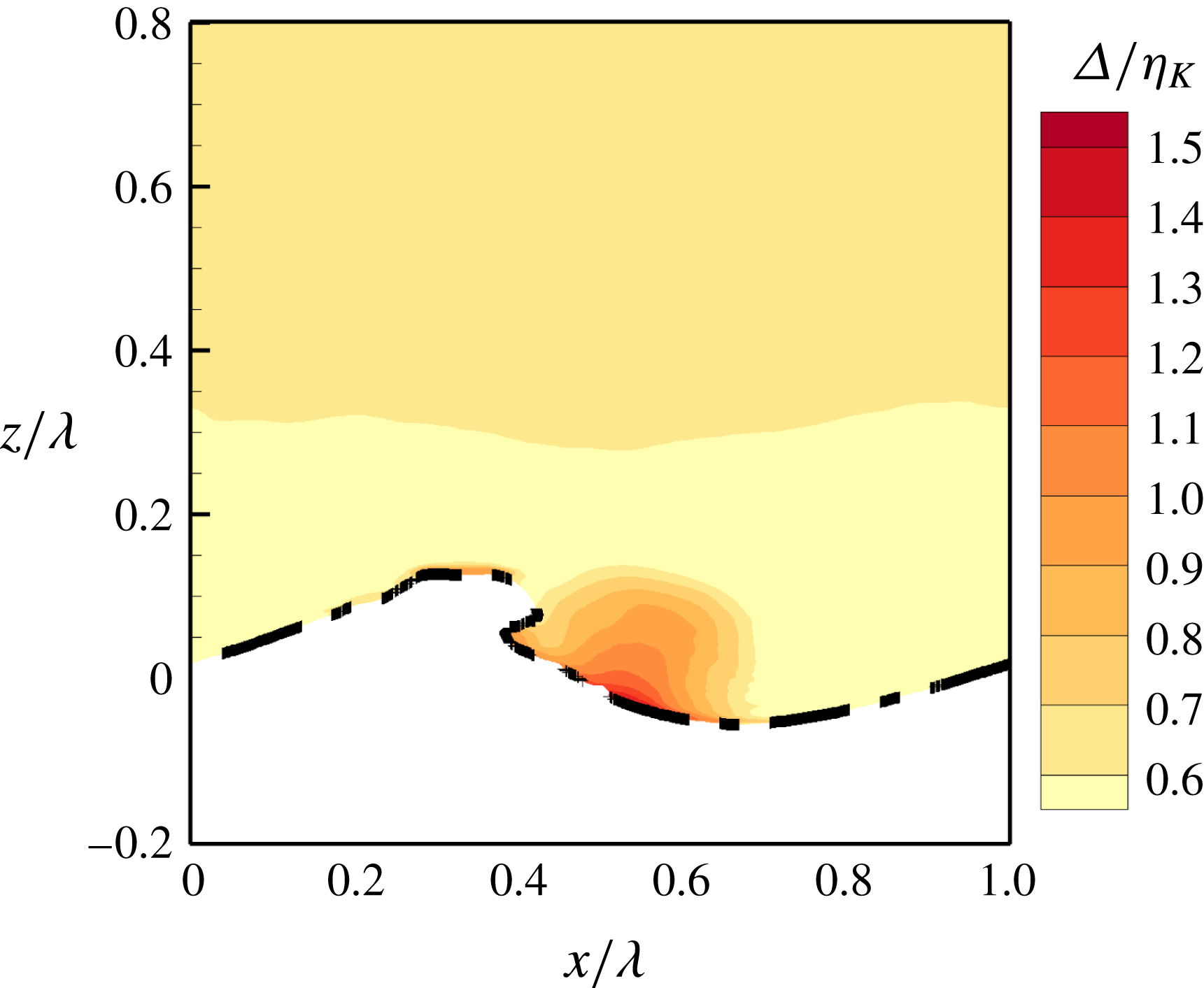
in case A55. The thick dash-dotted line represents the upper bound of wave surfaces.
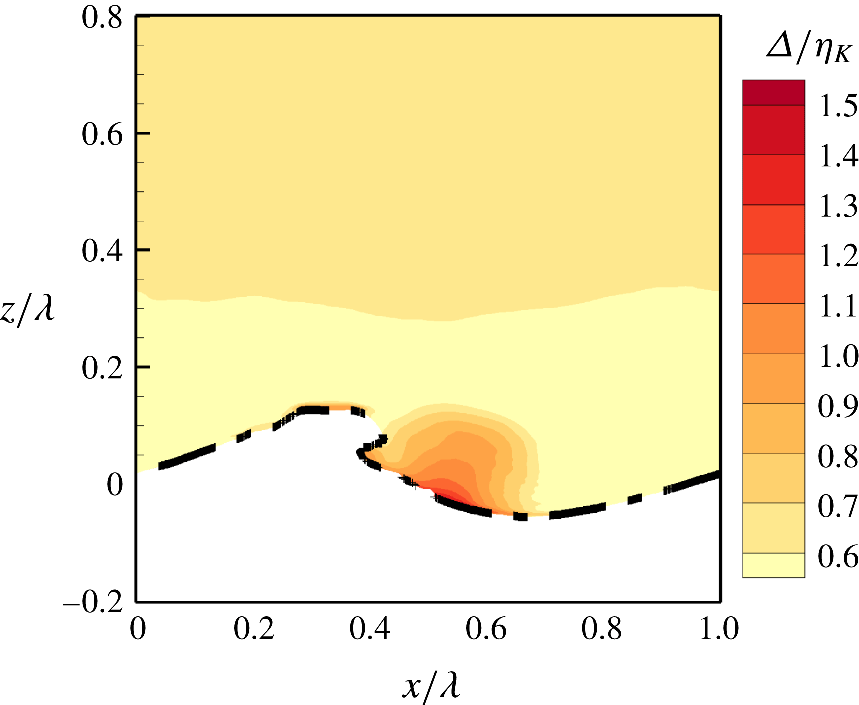
We have examined the grid resolution to confirm that it is sufficient for performing DNS of wind over breaking waves. Figure 3 displays the contours of the ratio between the grid size
 $\unicode[STIX]{x1D6E5}=(\unicode[STIX]{x1D6E5}_{x}\unicode[STIX]{x1D6E5}_{y}\unicode[STIX]{x1D6E5}_{z})^{1/3}$
and Kolmogorov length scale
 $\unicode[STIX]{x1D702}_{K}=(\unicode[STIX]{x1D708}_{a}^{3}/\unicode[STIX]{x1D716})^{1/4}$
at
 $t=0.8T$
in case A55. Here,
 $\unicode[STIX]{x1D716}=\unicode[STIX]{x1D708}\overline{\unicode[STIX]{x1D622}_{ij}^{\prime \prime }\unicode[STIX]{x1D622}_{ij}^{\prime \prime }}$
is the dissipation rate of turbulence kinetic energy (TKE), with
 $\unicode[STIX]{x1D622}_{ij}^{\prime \prime }=\unicode[STIX]{x2202}u_{i}^{\prime \prime }/\unicode[STIX]{x2202}x_{j}$
being the fluctuation of the velocity gradient tensor. It is demonstrated in figure 3 that the value of
 $\unicode[STIX]{x1D6E5}/\unicode[STIX]{x1D702}_{K}$
is smaller than
 $1.4$
in the bulk of air. We have also examined the grid resolution at different instants (from
 $t=0$
to
 $t=3.0T$
with an interval of
 $0.1T$
) in all simulation cases listed in table 1. The maximum of
 $\unicode[STIX]{x1D6E5}/\unicode[STIX]{x1D702}_{K}$
is smaller than 1.6, indicating that the grid resolution of the DNS is satisfied in the present study (Eswaran & Pope Reference Eswaran and Pope1988). Because we focus on the airflow in the present study, we show only the resolution in the air phase. In fact, the grid resolution normalized by the Kolmogorov scale is more adequate in water than in air due to the lower Reynolds number in water.
We note here that the instantaneous wave surface varies with the spanwise coordinate
 $y$
. Moreover, it differs among different ensemble runs. Therefore, the air–water interfaces should not be represented deterministically by a single line in a 2-D plot of ensemble-averaged statistics. In this paper, we use a thick dash-dotted line to denote the upper bound of all interfaces (figure 3). There are different approaches for defining the upper bound. The most strict definition corresponds to
 $\bar{\unicode[STIX]{x1D713}}=0$
, above which no water is found in any spanwise plane and in any sample. However, as pointed out by Brocchini & Peregrine (Reference Brocchini and Peregrine2001), because some small water droplets can be convected far away from the wave surface, it is more practical to use
 $\bar{\unicode[STIX]{x1D713}}=0.05$
to define the upper bound, which is adopted in the present study. In the region between the upper and lower bounds of the interfaces, the mean density is the fractional-averaged value of the densities of air and water, which varies spatially. In this sense, the flow is statistically compressible in this region (Hong & Walker Reference Hong and Walker2000; Chassaing et al.
Reference Chassaing, Antonia, Anselmet, Joly and Sarkar2002; Hendrickson et al.
Reference Hendrickson, Weymouth, Banerjee and Yue2013). Because we focus on the airflow in the present study, we only consider the flow field above the upper bound to reduce the complexity of the transport equations of the mean velocity and TKE.
4.3 Instantaneous wave surface
The process of wave breaking has been described in many papers (e.g. Duncan Reference Duncan1981, Reference Duncan1983; Longuet-Higgins Reference Longuet-Higgins1982; Bonmarin Reference Bonmarin1989; Chen et al. Reference Chen, Kharif, Zaleski and Li1999; Tulin & Waseda Reference Tulin and Waseda1999; Iafrati Reference Iafrati2009; Deike et al. Reference Deike, Popinet and Melville2015). The geometries of plunging and spilling breakers obtained from the present simulations are consistent with those observed in previous numerical simulations (Chen et al. Reference Chen, Kharif, Zaleski and Li1999; Iafrati Reference Iafrati2009; Deike et al. Reference Deike, Popinet and Melville2015; Lubin & Glockner Reference Lubin and Glockner2015). We demonstrate representative 3-D wave surfaces at different stages of wave breaking in this section. The plunging and spilling breakers are described based on cases A55 and A35, respectively.
Successive snapshots of instantaneous wave surface of plunging breakers in case A55. The waves propagate from left to right.
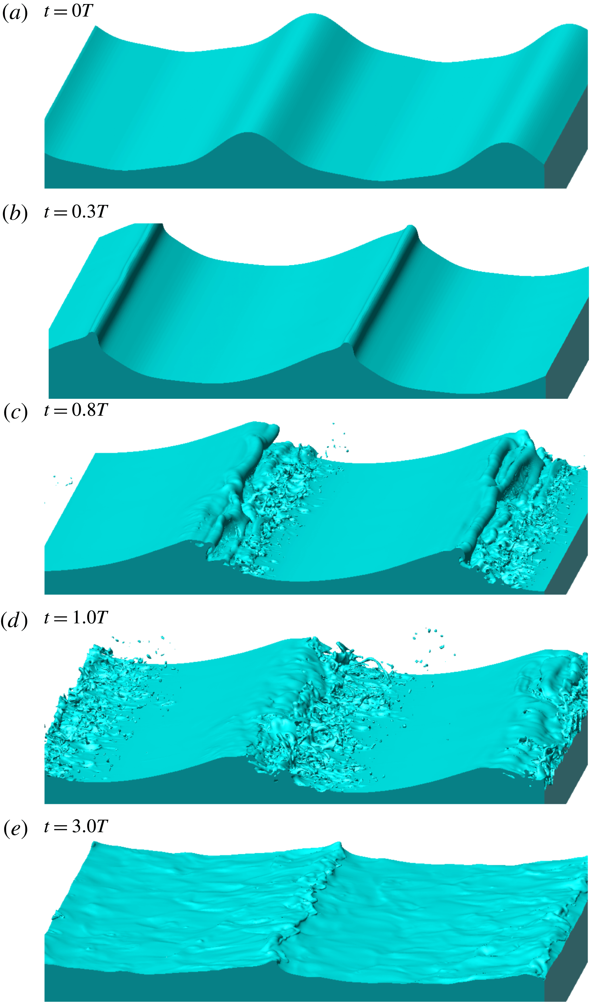
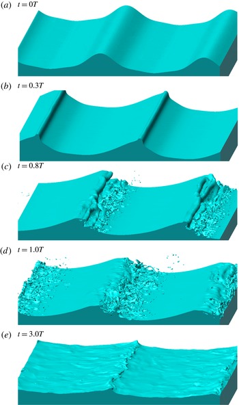
Figure 4 shows successive snapshots of instantaneous wave surfaces visualized using the isosurface of
 $\unicode[STIX]{x1D719}=0$
in case A55. The initial geometry of the wave surface is plotted in figure 4(a). The wave front is steepened and becomes almost vertical at
 $t=0.3T$
(figure 4
b). An overturning jet is then formed at the wave front at
 $t=0.8T$
(figure 4
c). The jet impinges onto the wave surface, causing splash-up events at
 $t=1.0T$
(figure 4
d). At
 $t=3.0T$
(figure 4
e), the waves keep breaking but the wave steepness is much smaller than that before the wave breaking (figure 4
a).
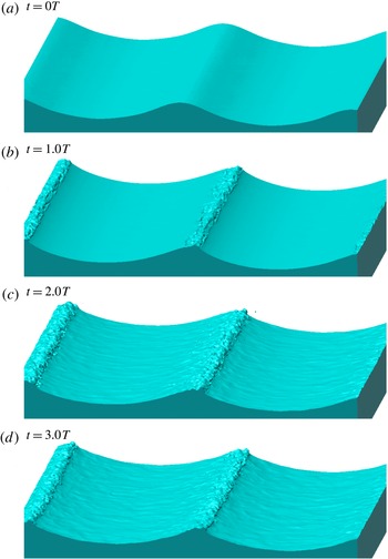
Successive snapshots of instantaneous wave surface of spilling breakers in case A35. The waves propagate from left to right.
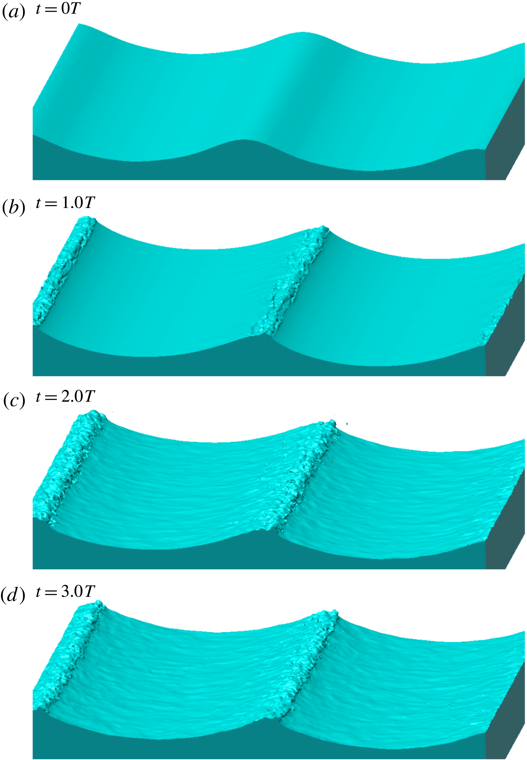
Figure 5 shows the characteristic snapshots of spilling breaking waves in case A35. Different from case A55, no overturning jet is generated in case A35. Instead, as displayed in figure 5(b), a bulge is formed when the wave front is steepened. Figure 5(c,d) shows that the bulge grows during wave breaking, and the wave surface is roughened behind (to the left in the figure) the wave crest.
4.4 Mean velocity
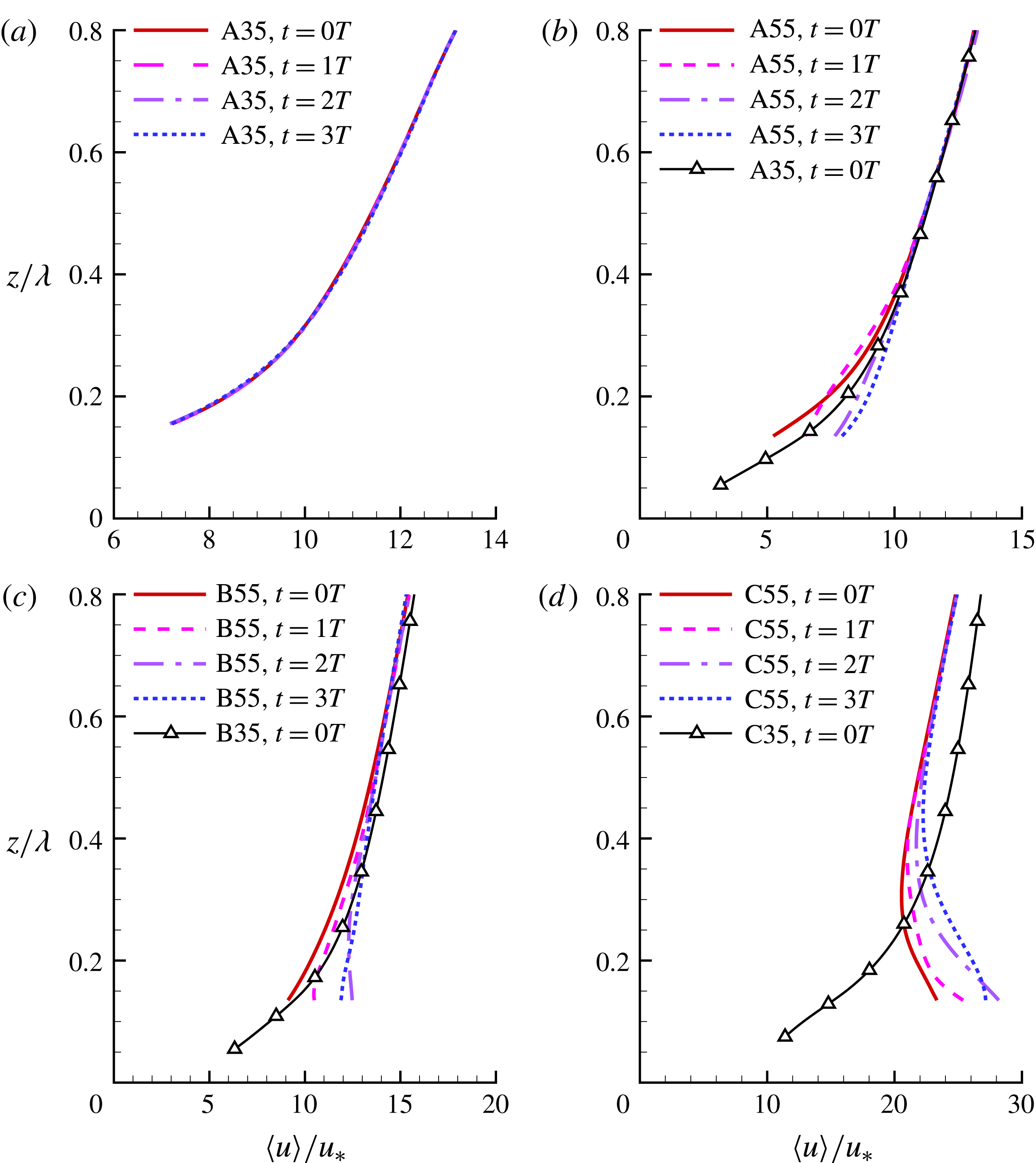
Vertical profiles of plane-averaged mean streamwise velocity
 $\langle u\rangle /u_{\ast }$
in cases (a) A35, (b) A55, (c) B55 and (d) C55. The results of cases A35, B35 and C35 at
 $t=0.0T$
are plotted respectively in (b–d) for comparison.

Figure 6(a) compares the vertical profiles of the plane-averaged mean streamwise velocity
 $\langle u\rangle$
normalized by
 $u_{\ast }$
at different time instants in case A35. Figure 6(b–d) shows respectively the vertical profiles of
 $\langle u\rangle /u_{\ast }$
in cases A55, B55 and C55, with the results in the respective cases A35, B35 and C35 at
 $t=0.0T$
superposed for comparison. Because the plane averaging is undefined below the wave crest, the lowest point of the profile is away from
 $z=0$
, which is different from the analyses of turbulence statistics on wave-surface-fitted grid (Hara & Sullivan Reference Hara and Sullivan2015). As shown in figure 6(a), the profile of
 $\langle u\rangle$
changes little during the spilling breaking process in case A35. Similarly, spilling breakers do not alter the profiles of
 $\langle u\rangle$
much in cases B35 and C35, so that we only show results at
 $t=0.0T$
in these two cases to keep the paper concise.
Figure 6(b) shows that at
 $t=0.0T$
, the magnitude of
 $\langle u\rangle$
below
 $z/\unicode[STIX]{x1D706}=0.4$
is slightly larger in case A35 than in case A55, but it is less sensitive to the wave steepness above
 $z/\unicode[STIX]{x1D706}=0.4$
. In the intermediate and old wave cases,
 $\langle u\rangle$
is more sensitive to the wave steepness. As demonstrated in figure 6(c), at
 $t=0.0T$
,
 $\langle u\rangle$
below
 $z/\unicode[STIX]{x1D706}=0.8$
is larger in case B35 than in case B55. Figure 6(d) shows that the profiles of
 $\langle u\rangle$
in cases C35 and C55 are drastically different. The vertical gradient of
 $\langle u\rangle$
is positive in case C35, but it is negative below
 $z/\unicode[STIX]{x1D706}=0.3$
in case C55. The negative velocity gradient near the wave surface is consistent with previous simulation results of wind over non-breaking waves at large wave age (Jiang et al.
Reference Jiang, Sullivan, Wang, Doyle and Vincent2016). A further discussion on the negative velocity gradient in case C55 is given in § 4.5.
Near the wave surface, the profiles of
 $\langle u\rangle$
in group I cases are sensitive to the violent plunging wave breaking. As demonstrated in figure 6(b–d), the magnitude of
 $\langle u\rangle$
near the wave surface is larger at
 $t=3.0T$
than at
 $t=0.0T$
in all of the three group I cases, indicating the overall transport of momentum from water to air during the wave plunging at various wave ages. However, it is observed in figure 6(b) that in case A55,
 $\langle u\rangle$
experiences a transient decrease above
 $z/\unicode[STIX]{x1D706}=0.2$
before
 $t=1.0T$
. Figure 6(c,d) shows respectively that in cases B55 and C55, the magnitude of
 $\langle u\rangle$
decreases slightly below
 $z/\unicode[STIX]{x1D706}=0.2$
after
 $t=2.0T$
. A further analysis on the response of
 $\langle u\rangle$
to the wave plunging is given in § 4.5 together with the total momentum flux
 $\langle u^{\prime }w^{\prime }\rangle$
.
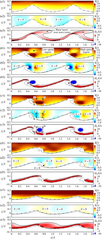
Phase-averaged flow field at (a)
 $t=0.0T$
, (b)
 $t=0.7T$
, (c)
 $t=0.8T$
, (d)
 $t=1.0T$
and (e)
 $t=3.0T$
in case A55. Mean streamwise velocity
 $\bar{u}$
, mean vertical velocity
 $\bar{w}$
, and mean spanwise vorticity
 $\unicode[STIX]{x1D714}_{y}$
are shown in panels 1, 2 and 3, respectively. The dotted line demonstrates an instantaneous air–water interface in a spanwise plane. The dash-dotted line represents the upper bound of all wave surfaces (see § 4.2 for the definition). The solid and dashed lines in panel 3 represent positive and negative isopleths of
 $\unicode[STIX]{x1D714}_{y}\unicode[STIX]{x1D706}/c$
, respectively. The interval of the isopleths is 5. The wave propagates in the
 $+x$
-direction.
Figure 7 shows the ensemble-averaged mean streamwise velocity
 $\bar{u}$
, mean vertical velocity
 $\bar{w}$
, and mean spanwise vorticity
 $\bar{\unicode[STIX]{x1D714}}_{y}$
near the wave surface at successive time instants in case A55. Note that the flow physics far away from the wave surface are dominated by wind, so that we use the characteristic velocity scale of wind
 $u_{\ast }$
to non-dimensionalize
 $\langle u\rangle$
in figure 6. In contrast, the effects of waves are dominant near the wave surface, and as a result, we use
 $c$
as the characteristic velocity scale in figure 7. As introduced in § 4.2, the thick dash-dotted line represents the upper bound of wave surfaces in different spanwise planes and simulation samples, which is different from instantaneous wave surface. For comparison, we also plot an instantaneous air–water interface at an
 $x$
–
 $z$
plane using the dotted line in figure 7. At
 $t=0.0T$
, the instantaneous wave surface collapses to the upper bound of interfaces, such that only the upper bound is shown in figure 7(a). It can be observed from figure 7(b–e) that at later times, the dotted lines are below the dash-dotted lines, which is expected based on the definition of the upper bound of interfaces given in § 4.2. Also note that as explained in § 3, ensemble-averaged quantities are defined in the region
 $[0,\unicode[STIX]{x1D706}]$
in the streamwise direction. Due to the use of the periodic boundary condition in the streamwise direction, we show the results in the region
 $[0,2\unicode[STIX]{x1D706}]$
by duplicating the flow field in
 $[0,\unicode[STIX]{x1D706}]$
to
 $[\unicode[STIX]{x1D706},2\unicode[STIX]{x1D706}]$
. This ensures that all flow structures can be demonstrated in a continuous frame.
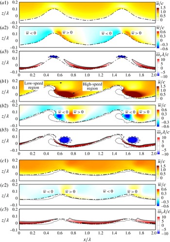
As demonstrated in figure 7(a2), when the wave is onset to break, the vertical velocity is negative and positive on the windward and leeward of the wave crest, respectively. This can be explained by the fact that the vertical component of the orbital velocity at the wave surface is positive on the leeward, and is negative on the windward. Therefore, the wave pushes the air on the leeward to move upward, while the air on the windward moves downward to follow the motion of the wave surface.
Figure 7(a3) shows that at
 $t=0.0T$
, the vorticity near the leeward of the wave surface is of small magnitude, and a shear layer detached from the wave surface appears in the downstream of the wave crest. This indicates that air particles do not move downward along the wave surface when they flow past the wave crest. Instead, they move upward, and a separation region is developed on the leeward of the wave surface. The airflow separation is consistent with observations from laboratory experiments (Banner & Melville Reference Banner and Melville1976; Reul et al.
Reference Reul, Branger and Giovanangeli1999; Veron et al.
Reference Veron, Saxena and Misra2007; Reul et al.
Reference Reul, Branger and Giovanangeli2008; Buckley & Veron Reference Buckley and Veron2016).
The overturning jet (figure 7 b,c) formed during the first plunging event alters the flow structures significantly. When the jet impinges onto the wave surface, it pushes the air to move forward. This process accelerates the airflow in the streamwise direction, and as a result, a high-speed region is developed ahead of the wave front (figure 7 b1,c1). Meanwhile, the jet brings the air particles around it to impinge onto the wave surface. Therefore, the vertical velocity of airflow displayed in figure 7(b2,c2) becomes negative on the leeward of the wave crest, and the airflow separation over the wave crest is weakened. This is evident from figure 7(b3,c3), which shows that the detached shear layer downstream of the wave crest is significantly weakened. Furthermore, figure 7(b2) shows that the upward-moving air on the leeward is pushed away from the wave surface, and a counterclockwise-rotating vortex is generated between the downward and upward airflow. This vortex corresponds to the negative vorticity in figure 7(b3,c3). The airflow above the vortex is decelerated to compensate the air moving downward with the jet, such that a low-speed region appears above the vortex (figure 7 b1,c1).
From the comparison between figure 7(a1,e1), it can be seen that the streamwise velocity above the wave crest increases during the wave breaking in case A55. This observation is consistent with the plane-averaged mean velocity
 $\langle u\rangle$
shown in figure 6(b). Two physical processes responsible for the acceleration of wind can be observed from figure 7. The first process corresponds to the air motion around the large-scale vortex. As illustrated in figure 7(c), when the airflow goes along the cycling routine ABCDA, the low-speed air moves downward with the jet from A to B, and is then accelerated from B to C. The high-speed air moves upward from C to D, losing momentum to the flow above the wave crest. Finally, the low-speed air moves back to point A (note that the mean streamwise velocity is positive in the earth frame plotted, but is negative in the frame travelling with the wave) and starts a new cycle. In this process, the vortex transports the high-speed air from the region ahead of the wave front to that above the wave crest. The second process lies in the fact that the velocity of water near the wave crest increases during wave breaking. Correspondingly, the air velocity above the wave crest is also accelerated. This is evident from figure 7(b1,c1), which shows that a high-speed region occurs over the wave crest. The two mechanisms are both associated with the first plunging event. As a result, the plane-averaged velocity near the wave crest increases more significantly before
 $t=1.0T$
than after that. For example, figure 6(b) shows that the value of
 $\langle u\rangle /u_{\ast }$
at
 $z/\unicode[STIX]{x1D706}=0.1$
increases by 48 % before
 $t=1.0T$
, whereas it increases by only 12 % after that.
Phase-averaged flow field at (a)
 $t=0.0T$
, (b)
 $t=0.8T$
and (c)
 $t=3.0T$
in case B55. See figure 7 for the detailed caption.

Figure 8 shows the ensemble-averaged mean streamwise velocity
 $\bar{u}$
, mean vertical velocity
 $\bar{w}$
and mean spanwise vorticity
 $\bar{\unicode[STIX]{x1D714}}_{y}$
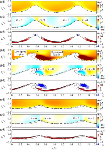
in case B55 for the wave with intermediate wave age (table 1). Figure 8(a1) does not show a shear layer over the wave crest in case B55 before the wave breaking, indicating that airflow separation is not evident at larger wave age. This is consistent with the observation in the laboratory experiment of Buckley & Veron (Reference Buckley and Veron2016). Similar to case A55, a spanwise vortex with negative
 $\bar{\unicode[STIX]{x1D714}}_{y}$
is generated during the first plunging event (figure 8
b3). From the comparison between figure 8(a1,c1), it is known that the mean velocity at the late stage of wave breaking (
 $t=3.0T$
) is slightly larger than that before wave breaking (
 $t=0.0T$
). Such an acceleration effect of wave breaking on the mean streamwise velocity is similar to that at small wave age in case A55.
Phase-averaged flow field at (a)
 $t=0.0T$
, (b)
 $t=0.8T$
and (c)
 $t=3.0T$
in case C55. See figure 7 for the detailed caption.

Figure 9 shows the ensemble-averaged flow field in case C55 with large wave age (table 1). Similar to case B55 (figure 8
a3), airflow separation is not evident in case C55 (figure 9
a3). As shown in figure 9(b3), the wave breaking also generates a spanwise vortex in case C55. From the comparison among figures 7(c1), 8(b1) and 9(b1), it can be seen that the streamwise scale of the high-speed region is larger in case C55 than in cases A55 and B55. The vortex also expands in the streamwise direction in case C55. It is known from the comparison between figure 9(a1,c1) that a plunging beaker with large wave age also causes the increase of the air velocity. This is consistent with the observation from figures 7 and 8 for cases A55 and B55, respectively, and is also consistent with the result of the plane-averaged mean velocity
 $\langle u\rangle$
shown in figure 6(d).
To further study the effect of wave breaking on the mean velocity, we analyse the transport equation of the integral mean velocity, which reads
 $$\begin{eqnarray}\displaystyle \frac{\unicode[STIX]{x2202}}{\unicode[STIX]{x2202}t}\int _{\unicode[STIX]{x1D6FA}}\overline{u}\,\text{d}V & = & \displaystyle \underbrace{-\int _{TB}\overline{uu_{ri}}n_{i}\,\text{d}s}_{C_{TB}}\underbrace{-\int _{TB}\frac{\bar{p}}{\unicode[STIX]{x1D70C}_{a}}n_{1}\,\text{d}s}_{\unicode[STIX]{x1D6F1}_{TB}}+\underbrace{\int _{TB}\unicode[STIX]{x1D708}_{a}\frac{\unicode[STIX]{x2202}\bar{u}}{\unicode[STIX]{x2202}x_{i}}n_{i}\,\text{d}s}_{D_{TB}}\nonumber\\ \displaystyle & & \displaystyle +\,\underbrace{\unicode[STIX]{x1D706}\langle uw\rangle |_{z_{1}}}_{C_{1}}+\underbrace{\unicode[STIX]{x1D706}\unicode[STIX]{x1D708}_{a}\left.\frac{\unicode[STIX]{x2202}\langle u\rangle }{\unicode[STIX]{x2202}z}\right|_{z_{1}}}_{D_{1}}.\end{eqnarray}$$
The equation above is derived by performing ensemble averaging on (2.2), and integrating the resultant equation in a control volume
 $\unicode[STIX]{x1D6FA}$
between the top bound (denoted by TB in the equation) of the wave surfaces and the horizontal plane at
 $z_{1}=0.14\unicode[STIX]{x1D706}$
, which is chosen to ensure that the wave crest is close but below it. It is shown in the following analyses that the evolution of the mean streamwise velocity near the wave surface is dominated by the momentum fluxes across the wave surface. Changing the value of
 $z_{1}$
does not alter our conclusions. Note that according to the definition of the ensemble averaging (3.2),
 $\unicode[STIX]{x1D6FA}$
is a 2-D geometry, while the top bound of wave surfaces and horizontal plane reduce to lines in (4.3). The left-hand side of (4.3) is the material derivative of the integral mean velocity. The first, second and third terms on the right-hand side of (4.3) are respectively the convection flux
 $C_{TB}$
, pressure flux
 $\unicode[STIX]{x1D6F1}_{TB}$
and viscous flux
 $D_{TB}$
across the top bound of wave surfaces, where
 $\boldsymbol{u}_{r}=[u_{r1},u_{r2},u_{r3}]$
is the relative velocity of airflow with respect to the moving speed of the top bound of wave surfaces, with
 $\boldsymbol{n}=[n_{1},n_{2},n_{3}]$
being its normal direction, pointing from air into water. Because the top bound of wave surfaces is not a material surface, fluid particles can cross it, resulting in a relative velocity between the airflow and top bound. However, this relative velocity is small, and as a result, the convection flux does not play a major role at the top bound of the wave surface, which is evident from the results shown below. The fourth and fifth terms on the right-hand side of (4.3) are respectively the convection flux
 $C_{1}$
and viscous flux
 $D_{1}$
across plane
 $z_{1}$
. Note that the definition of the plane averaging (3.5) is used to derive the last two terms.
Time history of momentum fluxes across the top bound of wave surfaces and horizontal plane at
 $z_{1}$
in cases (a) A35, (b) A55, (c) B55 and (d) C55.

Phase-averaged pressure field near the wave surface in case A55 at (a)
 $t=0.0T$
and (b)
 $t=0.6T$
. The pressure is normalized by
 $\unicode[STIX]{x1D70C}_{a}c^{2}$
. The thick dashed-dotted line represents the top bound of wave surfaces (see § 4.2 for the definition). The waves propagate in the
 $+x$
-direction.

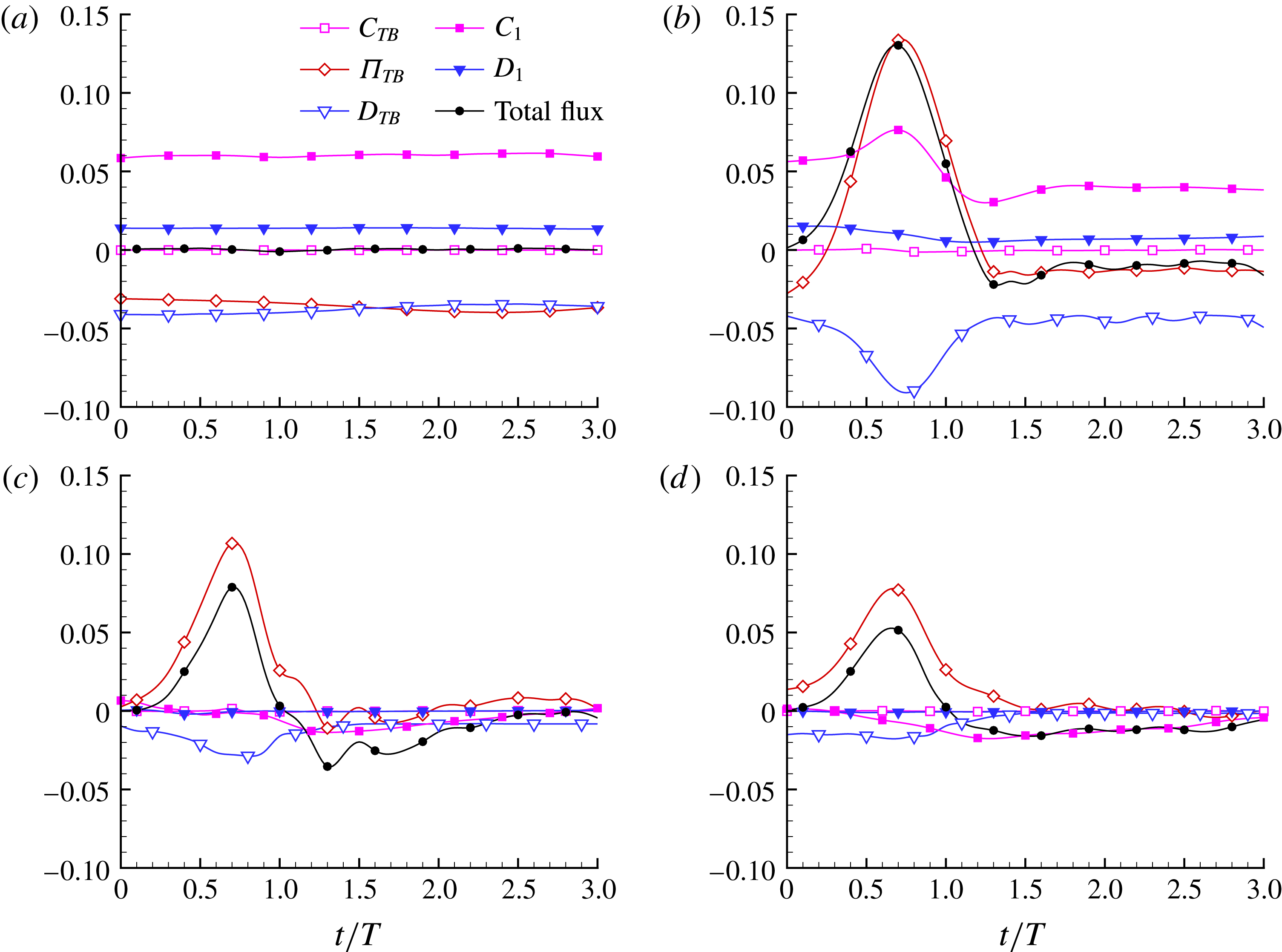
Figure 10 compares the time series of the flux terms on the right-hand side of equation (4.3) in cases A35, A55, B55 and C55. The total flux is also shown in the figure. All fluxes in figure 10 are normalized using
 $\unicode[STIX]{x1D706}c^{2}$
. At
 $t=0.0T$
, the initial field is a fully developed turbulent flow, so that the total flux is negligibly small, i.e. the flux terms are balanced, in all cases. In cases A35 and A55 (figure 10
a,b) for young waves, the pressure flux at the top bound of wave surface
 $\unicode[STIX]{x1D6F1}_{TB}$
is negative. In case B55 for the intermediate waves (figure 10
c), the magnitude of
 $\unicode[STIX]{x1D6F1}_{TB}$
becomes significantly smaller. In case C55 (figure 10
d) for the old waves,
 $\unicode[STIX]{x1D6F1}_{TB}$
reverses its sign to be positive. It has also been reported in the literature of wind over non-breaking waves (Sullivan et al.
Reference Sullivan, McWilliams and Moeng2000; Yang & Shen Reference Yang and Shen2010) that the value of pressure flux at the wave surface increases as the wave age increases.
Figure 10(a) shows that all fluxes change little during wave breaking in case A35 with spilling breakers. As a result, the mean streamwise velocity
 $\langle u\rangle$
shown in figure 6(a) does not change much. In contrast, with plunging breakers, the total flux increases rapidly before
 $t=0.7T$
in cases A55, B55 and C55. The pressure flux is the dominant term that causes the increase of the total flux. As shown in figure 10(b–d), the pressure flux increases significantly after
 $t=0.3T$
. To further explore the physical process responsible for the increase of the pressure flux across the wave surface, we compare the ensemble-averaged pressure at
 $t=0.0T$
and
 $t=0.6T$
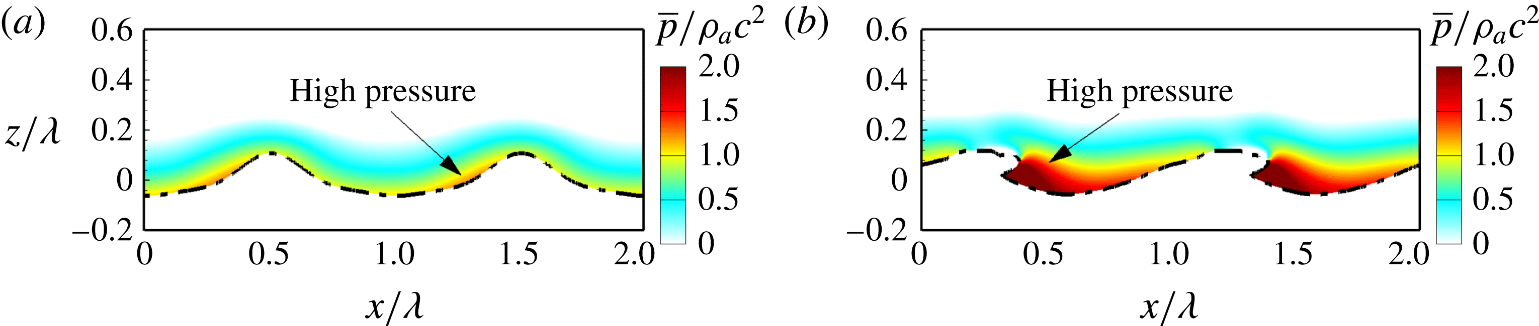
in case A55 in figure 11. It can be observed that at
 $t=0.0T$
, the pressure on the windward is higher than that on the leeward, which results in a form drag on the wind over steep waves. When the overturning jet is formed at
 $t=0.6T$
, as shown in figure 11(b), the pressure on the leeward increases significantly. This can be explained by the fact that the overturning jet increases the air pressure significantly to push the downstream air to move forward (see also figure 7
b1). The pressure field demonstrated in figure 11(b) explains why the pressure flux changes its sign to become positive during wave plunging.
At the horizontal plane
 $z_{1}$
, both the convection flux
 $C_{1}$
and viscous flux
 $D_{1}$
are positive in case A55 (figure 10
b), indicating that the air near the wave surface gains momentum from the air above this plane. The magnitude of
 $D_{1}$
decreases after the wave breaking, consistent with the observation from figure 6(b) that the vertical gradient of mean velocity
 $\unicode[STIX]{x2202}\langle u\rangle /\unicode[STIX]{x2202}z$
decreases during wave breaking in case A55. The magnitude of
 $C_{1}$
also decreases, indicating that the turbulence is suppressed there. Figure 10(c,d) shows respectively that in cases B55 and C55,
 $D_{1}$
is relatively small compared with the other fluxes. The value of
 $C_{1}$
is positive before wave breaking, characterizing a downward momentum flux. However,
 $C_{1}$
becomes negative at
 $t=0.8T$
and
 $t=0.3T$
in cases B55 and C55, respectively, indicating that the mean momentum gained from the pressure flux at the top bound of wave surfaces is transported to higher altitudes.
4.5 Momentum flux
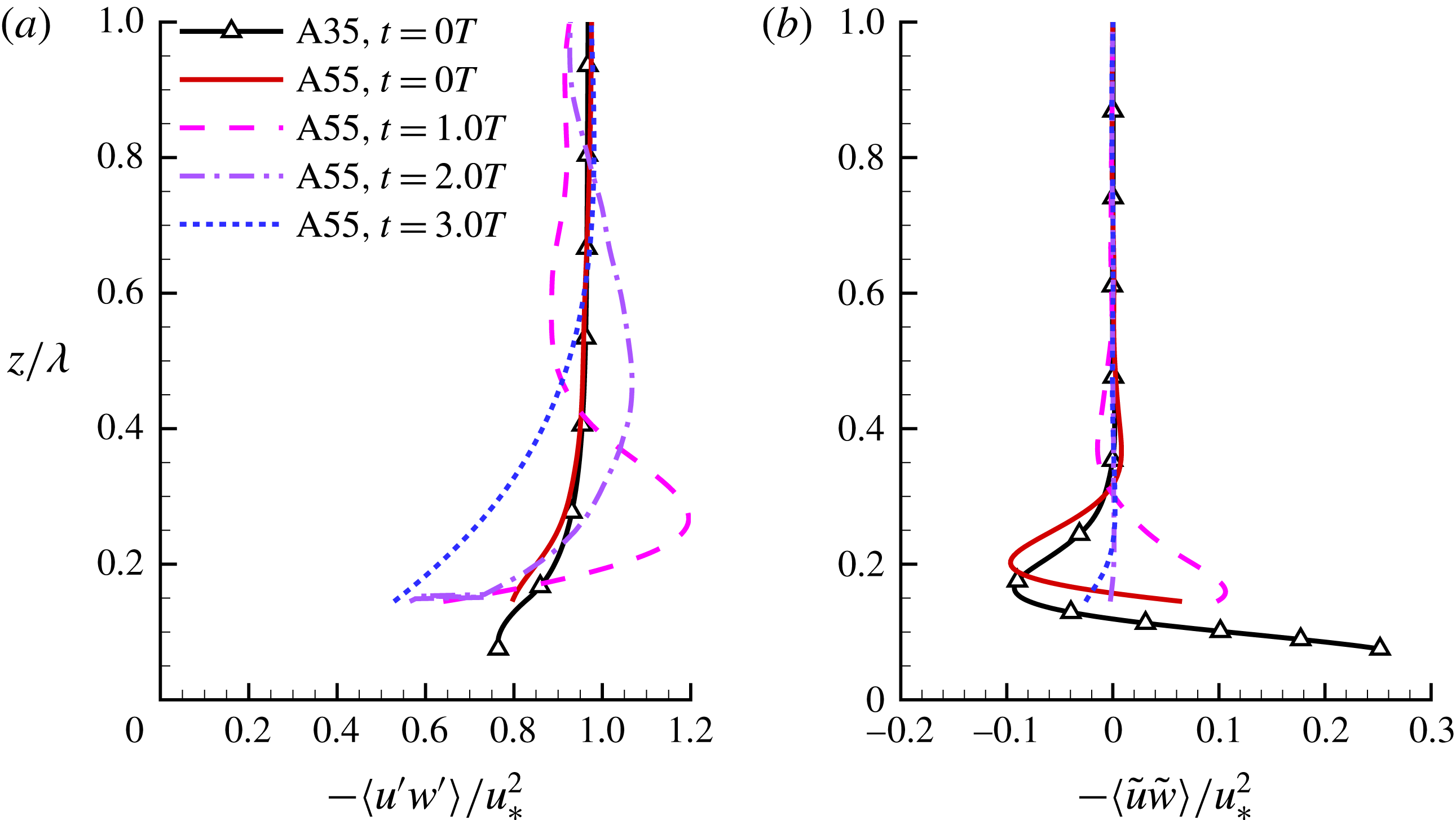
Vertical profiles of (a) plane-averaged total momentum flux
 $-\langle u^{\prime }w^{\prime }\rangle /u_{\ast }^{2}$
and (b) wave-coherent momentum flux
 $-\langle \tilde{u} \tilde{w}\rangle /u_{\ast }^{2}$
in case A55 at
 $t=0.0T$
,
 $1.0T$
,
 $2.0T$
and
 $3.0T$
. The result of case A35 at
 $t=0.0T$
is plotted for comparison.

The plane-averaged total momentum flux
 $-\langle u^{\prime }w^{\prime }\rangle$
plays an important role in the evolution of the plane-averaged mean streamwise velocity, of which the governing equation reads
 $$\begin{eqnarray}\displaystyle \frac{\unicode[STIX]{x2202}\langle u\rangle }{\unicode[STIX]{x2202}t}=\unicode[STIX]{x1D708}\frac{\unicode[STIX]{x2202}^{2}\langle u\rangle }{\unicode[STIX]{x2202}z^{2}}-\frac{\unicode[STIX]{x2202}\langle u^{\prime }w^{\prime }\rangle }{\unicode[STIX]{x2202}z}. & & \displaystyle\end{eqnarray}$$
Figure 12 compares the profiles of
 $-\langle u^{\prime }w^{\prime }\rangle$
and its wave-coherent part
 $-\langle \tilde{u} \tilde{w}\rangle$
in case A55. The result of case A35 at
 $t=0.0T$
is superimposed for comparison. At
 $t=0.0T$
, the profiles of
 $-\langle u^{\prime }w^{\prime }\rangle$
in cases A35 and A55 are close to each other, especially in the region away from the wave surface. As introduced in § 3, the initial field of the simulation is the fully developed wind turbulence over prescribed waves. In this statistically steady flow field, the left-hand side of (4.4) is trivial, and as a result, equation (4.4) can be further simplified to
 $$\begin{eqnarray}\displaystyle \unicode[STIX]{x1D708}\frac{\unicode[STIX]{x2202}\langle u\rangle }{\unicode[STIX]{x2202}z}-\langle u^{\prime }w^{\prime }\rangle =u_{\ast }^{2}. & & \displaystyle\end{eqnarray}$$
Figure 6(b) shows that
 $\unicode[STIX]{x2202}\langle u\rangle /\unicode[STIX]{x2202}z$
decreases as
 $z/\unicode[STIX]{x1D706}$
increases and becomes negligibly small far away from the wave surface. Therefore, as expected, it is observed from figure 12(a) that the value of
 $-\langle u^{\prime }w^{\prime }\rangle /u_{\ast }^{2}$
at
 $t=0.0T$
increases and approaches 1.0 as
 $z/\unicode[STIX]{x1D706}$
increases. This trend is consistent with the results of wind over non-breaking young waves in the literature (e.g. Sullivan et al.
Reference Sullivan, McWilliams and Moeng2000; Yang & Shen Reference Yang and Shen2010; Druzhinin et al. Reference Druzhinin, Troitskaya and Zilitinkevich2012; Sullivan et al.
Reference Sullivan, McWilliams and Patton2014).
The first plunging event disturbs the air near the wave surface, in a peak in the profile of
 $-\langle u^{\prime }w^{\prime }\rangle$
near
 $z/\unicode[STIX]{x1D706}=0.27$
at
 $t=1.0T$
(figure 12
a). Below and above this peak, the value of
 $-\unicode[STIX]{x2202}\langle u^{\prime }w^{\prime }\rangle /\unicode[STIX]{x2202}z$
is positive and negative, respectively. Because the viscous shear stress is less important than
 $-\langle u^{\prime }w^{\prime }\rangle$
in this region, it is understood from (4.4) that during wave breaking, the wind speed
 $\langle u\rangle$
is accelerated and decelerated below and above the peak of
 $-\langle u^{\prime }w^{\prime }\rangle$
, respectively. The peak of
 $-\langle u^{\prime }w^{\prime }\rangle$
moves upward with its magnitude decreasing after
 $t=1.0T$
, leading to an expansion of the acceleration region. As a result, the mean velocity increases after
 $t=1.0T$
(figure 6
b).
Figure 12(b) shows that at
 $t=0.0T$
, the value of
 $-\langle \tilde{u} \tilde{w}\rangle$
is positive near the wave crest height in case A55. It becomes negative above
 $z/\unicode[STIX]{x1D706}=0.15$
, and diminishes away from the wave surface (
 $z/\unicode[STIX]{x1D706}>0.3$
), indicating that the wave-coherent motion is confined in the near-surface region. At
 $t=1.0T$
, the value of
 $-\langle \tilde{u} \tilde{w}\rangle$
above the wave crest becomes positive. After
 $t=2.0T$
, the magnitude of
 $-\langle \tilde{u} \tilde{w}\rangle$
becomes negligibly small. Although the profile of
 $-\langle \tilde{u} \tilde{w}\rangle$
experiences a drastic change during wave breaking in case A55, it should not be regarded as the main reason for the occurrence of the peak in the profile of
 $-\langle u^{\prime }w^{\prime }\rangle$
, because the magnitude of
 $-\langle \tilde{u} \tilde{w}\rangle$
is much smaller than that of
 $-\langle u^{\prime }w^{\prime }\rangle$
. In the presence of wave plunging, the turbulence momentum flux (or, Reynolds stress) plays a much more important role than the wave-coherent momentum flux.
Vertical profiles of (a) plane-averaged total momentum flux
 $-\langle u^{\prime }w^{\prime }\rangle /u_{\ast }^{2}$
and (b) wave-coherent momentum flux
 $-\langle \tilde{u} \tilde{w}\rangle /u_{\ast }^{2}$
in case B55 at
 $t=0.0T$
,
 $1.0T$
,
 $2.0T$
and
 $3.0T$
. The result of case B35 at
 $t=0.0T$
is plotted for comparison.

Vertical profiles of (a) plane-averaged total momentum flux
 $-\langle u^{\prime }w^{\prime }\rangle /u_{\ast }^{2}$
and (b) wave-coherent momentum flux
 $-\langle \tilde{u} \tilde{w}\rangle /u_{\ast }^{2}$
in case C55 at
 $t=0.0T$
,
 $1.0T$
,
 $2.0T$
and
 $3.0T$
. The result of case C35 at
 $t=0.0T$
is plotted for comparison.

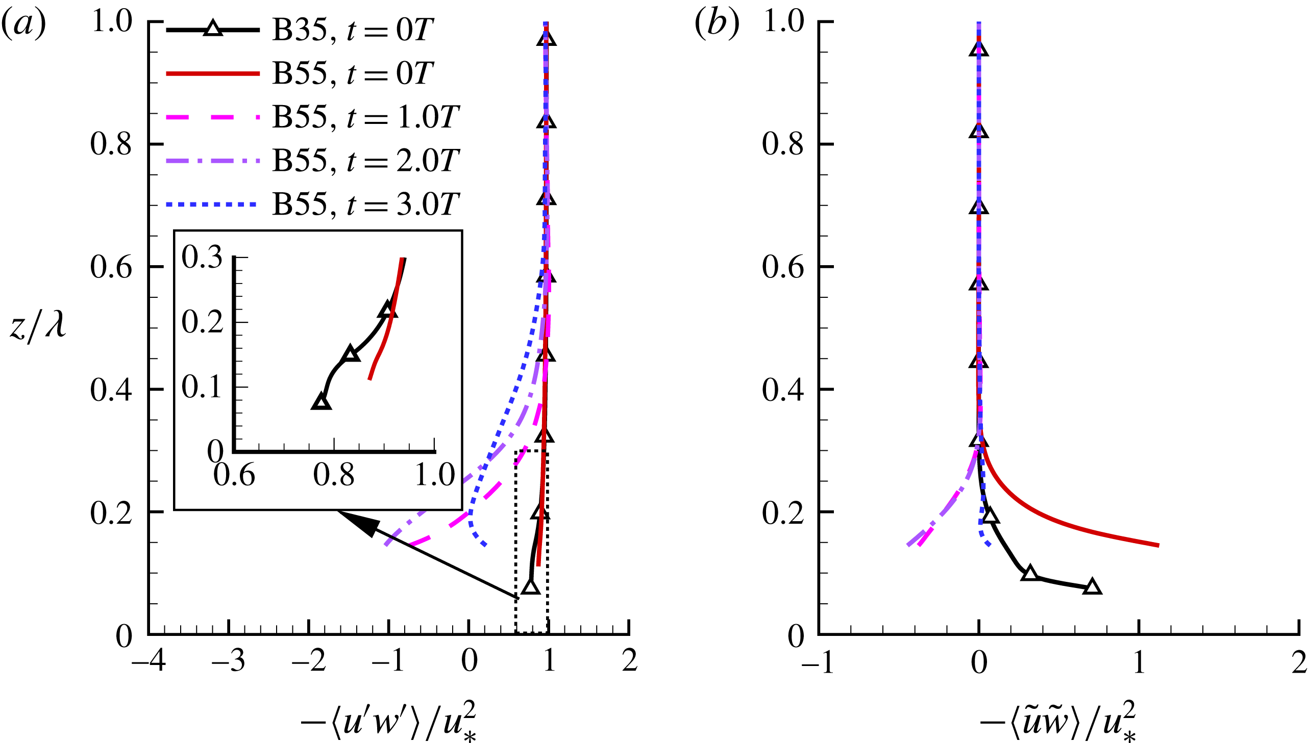
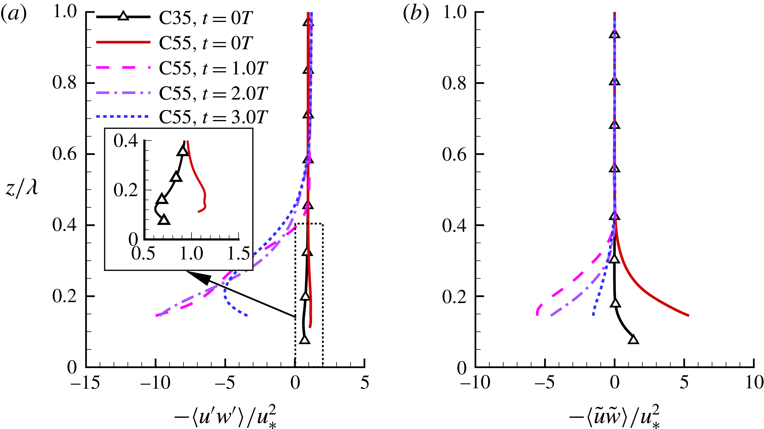
Figures 13 and 14 show the vertical profiles of
 $-\langle u^{\prime }w^{\prime }\rangle$
and
 $-\langle \tilde{u} \tilde{w}\rangle$
in cases B55 and C55, respectively. At
 $t=0.0T$
, the value of
 $-\langle u^{\prime }w^{\prime }\rangle$
near the wave surface is larger in cases B55 and C55 than in cases B35 and C35, respectively. In case C55, the value of
 $-\langle u^{\prime }w^{\prime }\rangle /u_{\ast }^{2}$
is larger than 1.0 below
 $z/\unicode[STIX]{x1D706}=0.30$
(figure 14
a). According to equation (4.5), this indicates that the value of
 $\unicode[STIX]{x2202}\langle u\rangle /\unicode[STIX]{x2202}z$
is negative, which is consistent with the observation from figure 6(d). At
 $t=1.0T$
, the value of
 $-\langle u^{\prime }w^{\prime }\rangle$
becomes negative in both cases B55 and C55. As discussed in § 4.4, this corresponds to the transport of momentum from the vicinity of the wave surface to the region away from the wave surface. At
 $t=3.0T$
, the value of
 $-\unicode[STIX]{x2202}\langle u^{\prime }w^{\prime }\rangle /\unicode[STIX]{x2202}z$
is negative below
 $z/\unicode[STIX]{x1D706}=0.2$
in cases B55 and C55. According to (4.4), this tends to decelerate the wind speed
 $\langle u\rangle$
near the wave surface, which is consistent with the results shown in figure 6(c,d).
A comparison among figures 12–14 indicates that the wave-coherent momentum flux
 $-\langle \tilde{u} \tilde{w}\rangle$
plays a more important role in cases B55 and C55 than in case A55. As shown in figure 13(b), the profile of
 $-\langle u^{\prime }w^{\prime }\rangle$
features a similar shape to that of
 $-\langle \tilde{u} \tilde{w}\rangle$
at
 $t=1.0T$
and
 $2.0T$
in case B55. In case C55, the contribution of
 $-\langle \tilde{u} \tilde{w}\rangle$
is more dominant. As shown in figure 14, the value of
 $-\langle \tilde{u} \tilde{w}\rangle /u_{\ast }^{2}$
is larger than 1.0 below
 $z/\unicode[STIX]{x1D706}=0.3$
. In response, the value of
 $-\langle u^{\prime }w^{\prime }\rangle /u_{\ast }^{2}$
also becomes larger than 1.0 in this region, which in turn leads to the negative value of
 $\unicode[STIX]{x2202}\langle u\rangle /\unicode[STIX]{x2202}z$
near the wave surface as shown in figure 6(d). At
 $t=1.0T$
and
 $2.0T$
, the magnitude of
 $-\langle \tilde{u} \tilde{w}\rangle$
is comparable to that of
 $-\langle u^{\prime }w^{\prime }\rangle$
in case C55, indicating that the evolution of
 $-\langle u^{\prime }w^{\prime }\rangle$
is dominated by the wave-coherent motion, when the wave age is large.
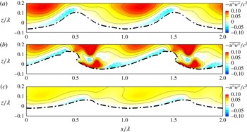
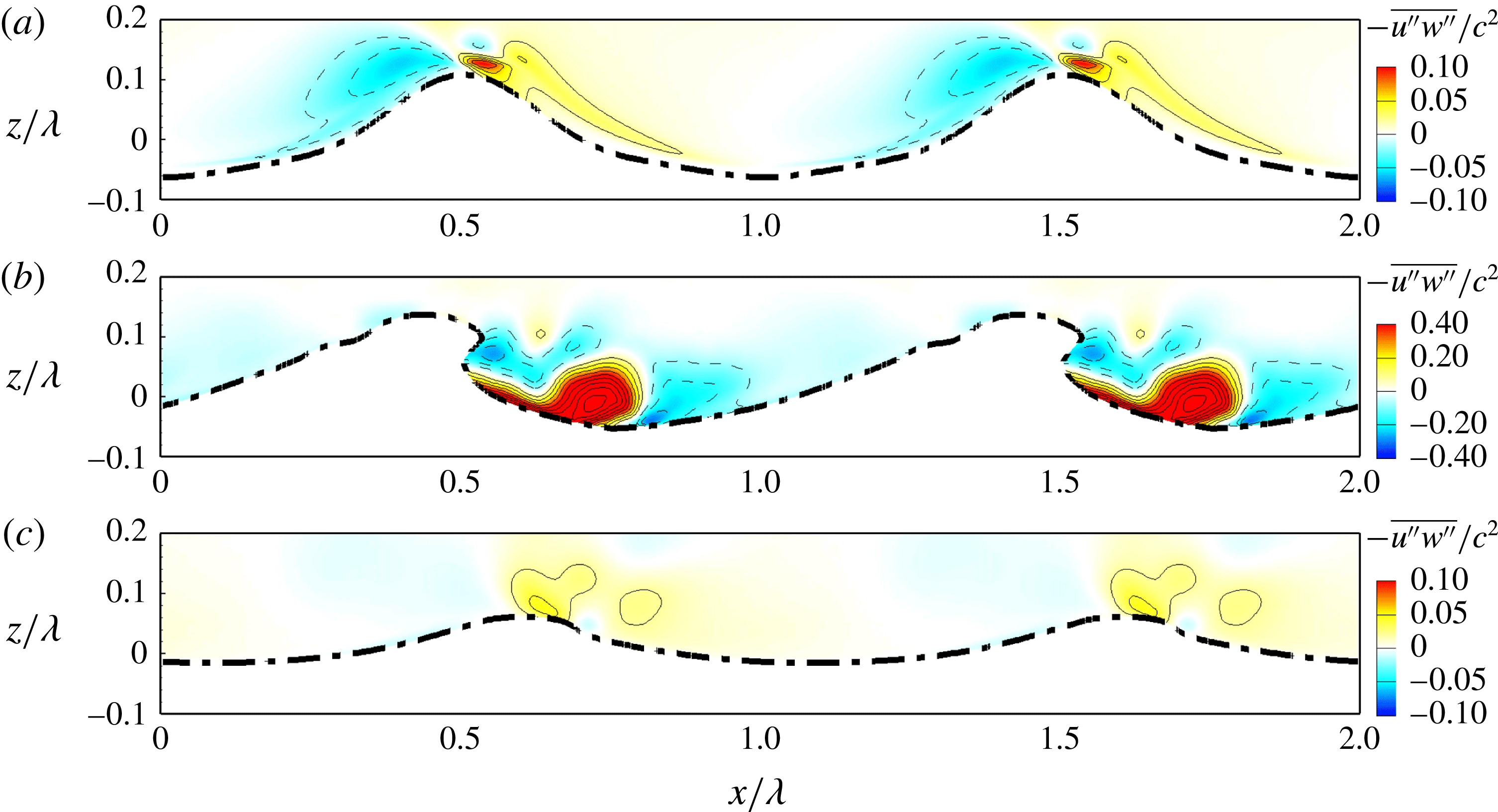
Contours of ensemble-averaged Reynolds shear stress
 $-\overline{u^{\prime \prime }w^{\prime \prime }}/c^{2}$
at (a)
 $t=0.0T$
, (b)
 $t=0.8T$
and (c)
 $t=3.0T$
in case A55. The solid and dashed lines represent isopleths of positive and negative values of
 $-\overline{u^{\prime \prime }w^{\prime \prime }}/c^{2}$
, respectively. The interval of the isopleths is 0.02. The thick dashed-dotted line represents the top bound of the wave surfaces (see § 4.2 for the definition). The waves propagate in
 $+x$
direction.

Figure 15 displays the contours of the ensemble-averaged Reynolds shear stress
 $-\overline{u^{\prime \prime }w^{\prime \prime }}$
near the wave surface in case A55. We recall here that the thick dashed-dotted line is the top bound of the wave surfaces, which is different from instantaneous wave surface. The definition of top bound of wave surface is given in § 4.2, and the top bound of the wave surfaces and instantaneous wave surface are compared in figures 7–9. Figure 15(a) shows that at
 $t=0.0T$
, the value of
 $-\overline{u^{\prime \prime }w^{\prime \prime }}$
is negative in a thin layer attached to the windward of the wave surface. Above this layer,
 $-\overline{u^{\prime \prime }w^{\prime \prime }}$
is positive, and a peak is located to the upper left of the windward of the wave surface. At
 $t=0.8T$
, the coherent vortex to the right of the wave crest enhances the momentum flux around it, and as a result, a large magnitude of
 $-\overline{u^{\prime \prime }w^{\prime \prime }}$
is observed around the vortex in figure 15(b). From the comparison between figure 15(a,c), it is known that the magnitude of
 $-\overline{u^{\prime \prime }w^{\prime \prime }}$
is smaller at
 $t=3.0T$
than at
 $t=0.0T$
, indicating that the turbulence is reduced after wave plunging. This is consistent with the results of the plane-averaged total momentum flux demonstrated in figure 12(a).
Contours of ensemble-averaged Reynolds shear stress
 $-\overline{u^{\prime \prime }w^{\prime \prime }}/c^{2}$
at (a)
 $t=0.0T$
, (b)
 $t=0.8T$
and (c)
 $t=3.0T$
in case B55. See figure 15 for the detailed caption.

Contours of ensemble-averaged Reynolds shear stress
 $-\overline{u^{\prime \prime }w^{\prime \prime }}/c^{2}$
at (a)
 $t=0.0T$
, (b)
 $t=0.8T$
and (c)
 $t=3.0T$
in case C55. See figure 15 for the detailed caption.

Figures 16 and 17 display the contours of the ensemble-averaged Reynolds shear stress
 $-\overline{u^{\prime \prime }w^{\prime \prime }}$
near the wave surface in cases B55 and C55, respectively. From the comparison among figures 15(a), 16(a) and 17(a), it can be seen that at
 $t=0.0T$
, the region with negative
 $-\overline{u^{\prime \prime }w^{\prime \prime }}$
on the windward of the wave expands as
 $c/u_{\ast }$
increases, and the positive and negative contours become more symmetric about the wave crest. The same trend of the ensemble-averaged Reynolds stress contours in response to the increase of
 $c/u_{\ast }$
has been reported by Yang & Shen (Reference Yang and Shen2010) for wind over non-breaking waves. Similar to that in case A55 (figure 15
b), the spanwise vortex induces large magnitude of
 $-\overline{u^{\prime \prime }w^{\prime \prime }}$
around it at
 $t=0.8T$
in cases B55 and C55 (figures 16
b and 17
b). The comparisons between figure 16(a,c) and between 17(a,c) show that the magnitude of
 $-\overline{u^{\prime \prime }w^{\prime \prime }}$
is slightly smaller at
 $t=3.0T$
than at
 $t=0.0T$
in both cases B55 and C55, indicating the reduction of turbulence after wave breaking. This is consistent with case A55 for young waves (figure 15
a,c).
4.6 Kinetic energy of velocity fluctuations
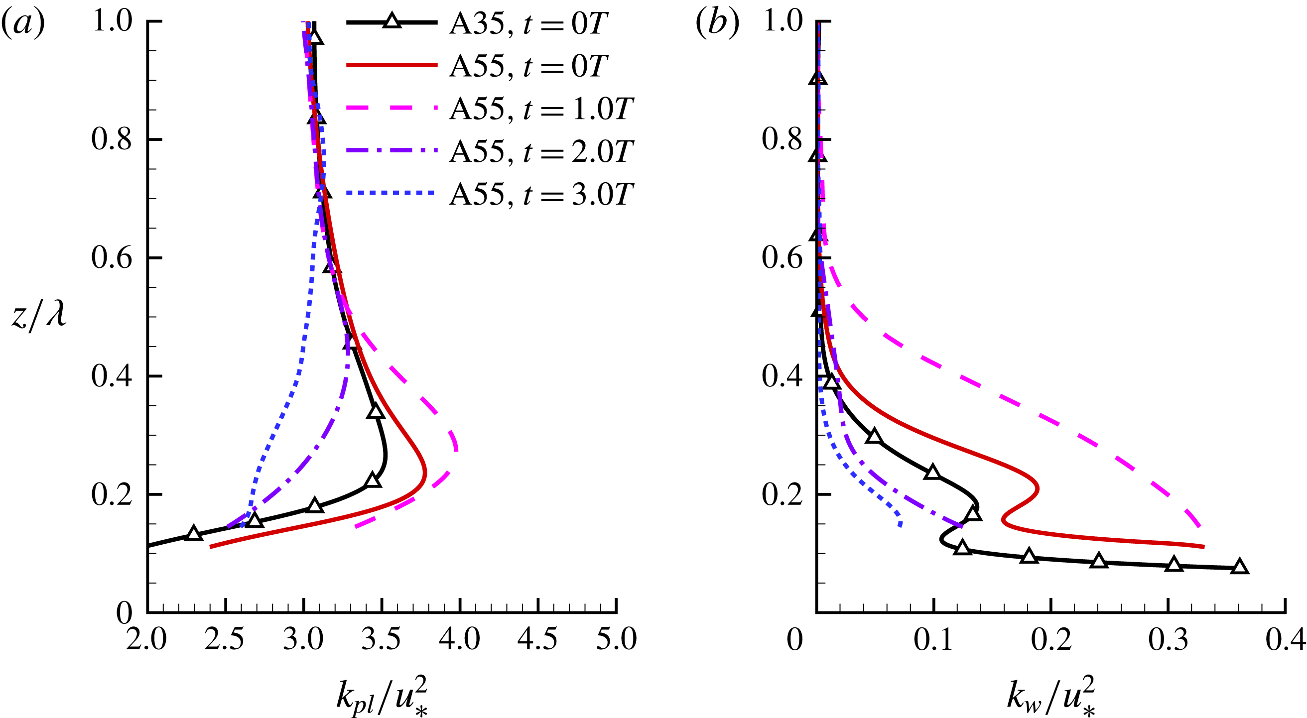
Vertical profiles of (a) plane-averaged KE-F
 $k_{pl}/u_{\ast }^{2}$
and (b) KE-W
 $k_{w}/u_{\ast }^{2}$
in case A55 at
 $t=0.0T$
,
 $1.0T$
,
 $2.0T$
and
 $3.0T$
. The result of case A35 at
 $t=0.0T$
is plotted for comparison.

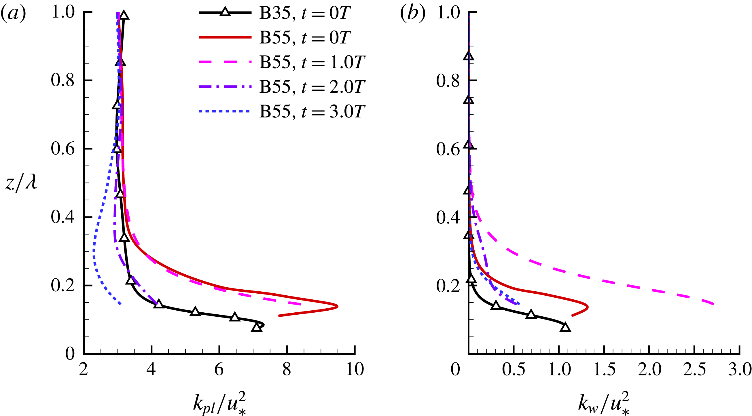
Vertical profiles of (a) plane-averaged KE-F
 $k_{pl}/u_{\ast }^{2}$
and (b) KE-W
 $k_{w}/u_{\ast }^{2}$
in case B55 at
 $t=0.0T$
,
 $1.0T$
,
 $2.0T$
and
 $3.0T$
. The result of case B35 at
 $t=0.0T$
is plotted for comparison.

Vertical profiles of (a) plane-averaged KE-F
 $k_{pl}/u_{\ast }^{2}$
and (b) KE-W
 $k_{w}/u_{\ast }^{2}$
in case C55 at
 $t=0.0T$
,
 $1.0T$
,
 $2.0T$
and
 $3.0T$
. The result of case C35 at
 $t=0.0T$
is plotted for comparison.

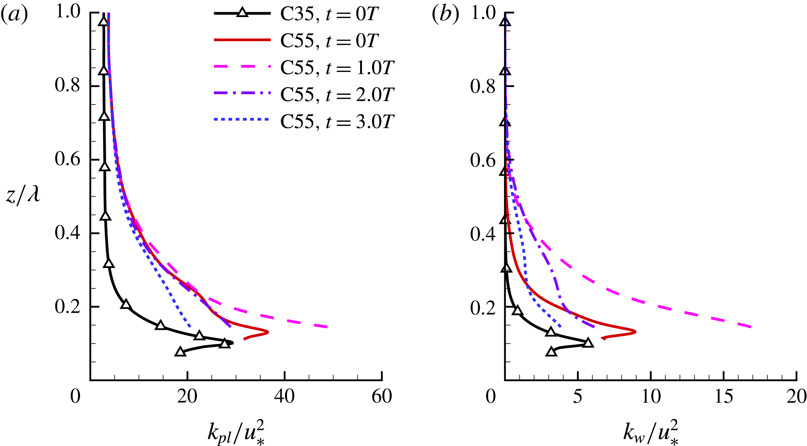
In this section, we further analyse the effect of wave breaking on the kinetic energy of velocity fluctuations (KE-F). Figures 18–20 compare the vertical profiles of the plane-averaged KE-F,
 $k_{pl}=\langle u_{i}^{\prime }u_{i}^{\prime }\rangle /2$
, and the kinetic energy of wave-coherent velocity (KE-W),
 $k_{w}=\langle \tilde{u} _{i}\tilde{u} _{i}\rangle /2$
, in cases with young waves (A35 and A55), intermediate waves (B35 and B55) and old waves (C35 and C55), respectively.
From the comparison between (a,b) in figures 18–20, it is known that the contribution from
 $k_{w}$
to
 $k_{pl}$
becomes more important as the wave age increases, consistent with the results of
 $-\langle u^{\prime }w^{\prime }\rangle$
and
 $-\langle \tilde{u} \tilde{w}\rangle$
displayed in figures 12–14. The wave steepness influences both
 $k_{pl}$
and
 $k_{w}$
near the wave surface. As shown in figures 18–20, at
 $t=0.0T$
, the magnitudes of
 $k_{pl}$
and
 $k_{w}$
in cases A55, B55 and C55 are respectively larger than those in cases A35, B35 and C35 below
 $z/\unicode[STIX]{x1D706}=0.4$
. However, the wave steepness does not influence the KE-F far away from the wave surface. This is consistent with the results of the mean velocity and total momentum flux demonstrated in figures 6, 12–14.
The wave plunging influences the KE-F near the wave surface significantly. As shown in figure 18(a), in case A55, the value of
 $k_{pl}$
below
 $z/\unicode[STIX]{x1D706}=0.55$
is higher at
 $t=1.0T$
than at
 $t=0.0T$
, indicating that the turbulence is transiently enhanced due to the wave breaking. The KE-F also experiences a transient growth in case C55. However, we do not observe such a transient growth of KE-F in case B55. The turbulence is eventually reduced after wave plunging ceases in cases A55, B55 and C55.
Vertical profile of plane-averaged KE-F production
 $P_{k}/(u_{\ast }^{3}/\unicode[STIX]{x1D706})$
in cases (a) A55, (b) B55 and (c) C55.

To further study why the transient growth of KE-F takes place in cases A55 and C55 but is absent in case B55, we compare the production of KE-F,
 $P_{k}$
, in these three cases in figure 21. Here,
 $P_{k}$
is defined as
 $$\begin{eqnarray}\displaystyle P_{k}=-\langle u^{\prime }w^{\prime }\rangle \frac{\unicode[STIX]{x2202}\langle u\rangle }{\unicode[STIX]{x2202}z}. & & \displaystyle\end{eqnarray}$$
The production term represents a rapid effect on the KE-F (Townsend Reference Townsend1980), and the behaviour of KE-F is often dominated by its production term (Mansour, Kim & Moin Reference Mansour, Kim and Moin1988; Smits, McKeon & Marusic Reference Smits, McKeon and Marusic2011). Note that the full production term of KE-F reads
 $$\begin{eqnarray}\displaystyle P_{k}=-\langle u_{i}^{\prime }u_{j}^{\prime }\rangle \frac{\unicode[STIX]{x2202}\langle u_{i}\rangle }{\unicode[STIX]{x2202}x_{j}}. & & \displaystyle\end{eqnarray}$$
However, according to the definition of plane averaging,
 $\unicode[STIX]{x2202}\langle \;\rangle /\unicode[STIX]{x2202}x=\unicode[STIX]{x2202}\langle \;\rangle /\unicode[STIX]{x2202}y=0$
holds theoretically. Furthermore, the magnitudes of the mean spanwise velocity
 $\langle v\rangle$
and mean vertical velocity
 $\langle w\rangle$
are negligibly small in comparison with the mean streamwise velocity
 $\langle u\rangle$
. As a result, the production of KE-F is simplified to (4.6).
It is evident from figure 21(a,c) that in cases A55 and C55, the magnitude of
 $P_{k}$
is larger at
 $t=1.0T$
than at
 $t=0.0T$
. However, the physical process leading to the increase of
 $P_{k}$
is different in these two cases. From equation (4.6), it is known that the value of
 $P_{k}$
is determined by the vertical gradient of mean velocity
 $\unicode[STIX]{x2202}\langle u\rangle /\unicode[STIX]{x2202}z$
and the total momentum flux
 $-\langle u^{\prime }w^{\prime }\rangle$
. In case A55,
 $\unicode[STIX]{x2202}\langle u\rangle /\unicode[STIX]{x2202}z$
decreases during the first plunging event (as can be seen from the
 $\langle u\rangle$
profile in figure 6
b), which tends to reduce the value of
 $P_{k}$
. On the opposite, the magnitude of
 $-\langle u^{\prime }w^{\prime }\rangle$
increases and a positive peak occurs in its profile (figure 12
a) due to the disturbance effect of the wave breaking on the turbulent flow, which tends to cause an increase of
 $P_{k}$
. Figure 21(a) indicates that the latter effect is stronger in the young wave case, and as a result
 $k_{pl}$
experiences a transient growth during the first plunging event (figure 18
a). In case C55, the transient growth of KE-F is correlated to the negative value of
 $\unicode[STIX]{x2202}\langle u\rangle /\unicode[STIX]{x2202}z$
near the wave surface (figure 6
d), which leads to a negative value of
 $P_{k}$
at
 $t=0.0T$
as shown in figure 21(c). During the first plunging event, because the wave breaking induces a large negative value of
 $-\langle \tilde{u} \tilde{w}\rangle$
(figure 14
b), the value of
 $-\langle u^{\prime }w^{\prime }\rangle$
becomes negative correspondingly (figure 14
a). As a result,
 $P_{k}$
becomes positive at
 $t=1.0T$
near the wave surface. Consequently, the magnitude of KE-F also increases transiently in case C55 during the first plunging event. In case B55, however, none of the two processes described above is present. As demonstrated in figure 13(a), no positive peak occurs in the profile of
 $-\langle u^{\prime }w^{\prime }\rangle$
during the first plunging event, while figure 6(c) shows that
 $\unicode[STIX]{x2202}\langle u\rangle /\unicode[STIX]{x2202}z$
is positive in case B55. Therefore, the turbulence does not experience a transient growth in this intermediate wave case. The production of KE-F is smaller at
 $t=3.0T$
than at
 $t=1.0T$
in all cases, which leads to the magnitude decrease of KE-F after wave plunging (figures 18
a, 19
a and 20
a).
Contours of ensemble-averaged TKE,
 $k_{ph}/c^{2}$
, at (a)
 $t=0.0T$
, (b)
 $t=0.8T$
and (c)
 $t=3.0T$
in case A55. The interval of the isopleths is 0.1. The thick dashed-dotted line represents the top bound of wave surfaces (see § 4.2 for the definition). The waves propagate in the
 $+x$
-direction.

Figure 22 displays the contours of the ensemble-averaged TKE,
 $k_{ph}=\overline{u_{i}^{\prime \prime }u_{i}^{\prime \prime }}/2$
, near the wave surface in case A55. As shown in figure 22(a), at
 $t=0.0T$
, the value of
 $k_{ph}$
is small near the leeward of the surface. Figure 22(b) shows that at
 $t=0.8T$
,
 $k_{ph}$
increases near the large spanwise vortex (cf. figure 7
c3), indicating that the turbulence is enhanced by the vortex. This is consistent with the result of
 $-\overline{u^{\prime \prime }w^{\prime \prime }}$
shown in figure 15(b). At
 $t=3.0T$
, as the turbulence is reduced, the magnitude of
 $k_{ph}$
is smaller than that at
 $t=0.0T$
.
Contours of ensemble-averaged TKE,
 $k_{ph}/c^{2}$
, at (a)
 $t=0.0T$
, (b)
 $t=0.8T$
and (c)
 $t=3.0T$
in case C55. The interval of isopleths is 0.02 in (a,c), while it is 0.1 in (b). The thick dashed-dotted line represents the top bound of wave surfaces (see § 4.2 for the definition). The waves propagate in the
 $+x$
-direction.

Figure 23 illustrates the contours of
 $k_{ph}$
near the wave surface in case C55. As shown in figure 23(a), the peak of
 $k_{ph}$
occurs near the wave surface at
 $t=0.0T$
. Similar to that in case A55, the magnitude of
 $k_{ph}$
increases significantly at
 $t=0.8T$
near the spanwise vortex (cf. figure 9
b3). The value of
 $k_{ph}$
near the vortex at
 $t=0.8T$
scales with
 $c^{2}$
in cases A55 and C55, indicating that the high TKE in this region is dominated by the wave breaking. At
 $t=3.0T$
, the magnitude of
 $k_{ph}$
near the wave surface becomes smaller than that at
 $t=0.0T$
. This is similar to the results of case A55 shown in figure 22.
The figures of
 $k_{ph}$
of case B55 are not shown here to keep the paper concise. Similar to that in cases A55 and C55, the magnitude of TKE in case B55 experiences an increase during the wave plunging near the wave surface, and is eventually reduced after the wave breaking. However, the TKE far away from the wave surface does not increase transiently in case B55 during wave plunging (figure 19
a). This indicates that although TKE is generated in the vicinity of the wave surface during wave plunging, little is transported to high altitude before it is dissipated. As shown above, the transient growth of KE-F away from the wave surface during wave plunging in cases A55 and C55 is caused by the large magnitude of local KE-F production.
5 Conclusions
In this study, direct numerical simulations are performed to study wind over breaking waves. The air and water are simulated as a coherent system, with the interfaced captured using the coupled level-set and volume-of-fluid method. Three wave ages and two initial wave steepness values are considered. Because wave breaking is an unsteady process, we conduct 100 runs for each case to perform ensemble averaging, of which the initial wind profile and wave geometry are the same, while the instantaneous turbulent fluctuations are different.
It is found that before wave breaking, the turbulence statistics are significantly influenced by the wave age. The vertical gradient of mean velocity is positive at small and medium wave ages, but at the large wave age, it becomes negative near the wave surface. This is because the pressure force changes from drag to thrust as the wave age increases. The contribution of the wave-induced motion to the total momentum flux and KE-F is relatively small at the small wave age, indicating that the flow physics of the airflow is dominated by the wind turbulence. In contrast, contribution of the wave-induced part becomes increasingly important as the wave age increases.
Wave spilling does not alter the wind turbulence significantly. In contrast, wave plunging induces substantial effects on the turbulence statistics and flow structures near the wave surface. During wave plunging, the overturning jet pushes the air to accelerate it in the streamwise direction. The pressure near the impinging jet increases significantly, leading to the momentum flux from water to air, which is in the opposite direction to that before wave breaking, when the steep wave exerts drag on the airflow. As a result, the wind speed near the wave surface is accelerated by the breaker. Meanwhile, a spanwise vortex rotating in the counterclockwise direction is generated, of which the streamwise extent increases as the wave age increases. The airflow near this large vortex is greatly disturbed, and in consequence, the magnitudes of the Reynolds shear stress and TKE near this large vortex are significantly amplified. At the small wave age, the turbulence above the wave crest experiences a transient enhancement during the first plunging event, which is characterized by the transient growth of the magnitude of KE-F. A further investigation of the KE-F production shows that this is caused by the peak occurring in the profile of the total momentum flux due to the disturbance effect of wave plunging. At the large wave age, the KE-F above the wave crest also increases during wave plunging. This is because the sign of the KE-F production changes from negative to positive during wave plunging, which results from the change in the sign of the wave-coherent momentum flux. Therefore, the processes leading to the transient increases of KE-F at small and large wave ages are different. At the intermediate wave age, both processes are absent, and no transient growth of KE-F is observed.
Finally, we remark that while the results shown in this paper indicate that DNS is a useful tool for mechanistic studies of small-scale physical processes associated with wind over breaking waves, it would be desirable to perform fine-resolution simulation of more realistic problems with the increase of computer power in the future. For example, the wave-focusing method might be used to generate breaking waves under the wind, such that the historical effect of wind on the wave geometry can be captured. This imposes a higher demand on the computing power, because the computational domain size needs to be significantly elongated in the streamwise direction. Furthermore, it would be desirable to assimilate laboratory and field measurement data into the simulation to help the set-up of more realistic simulations. These research directions will be the pursuits in our future studies.
Acknowledgements
This work is supported by Office of Naval Research and Minnesota Sea Grant. The authors would like to thank Professors J. Duncan and F. Veron for the helpful discussion on the results.