1 Introduction
Stars of mass above 2.5 solar masses (
 $2.5M_{\odot }$
), also known as early type stars, are basically made of a central convective core (where nuclear reactions take place) and a radiative envelope. When the star is rapidly rotating, as it is often the case for this type of stars, the radiative envelope is differentially rotating as a result of the baroclinic torque that comes from the stable stratification in the envelope (Zahn Reference Zahn1992; Rieutord Reference Rieutord2006). Besides, the envelope is the seat of oscillations driven by the so-called
 ${\it\kappa}$
-mechanism (Zhevakin Reference Zhevakin1963; Unno et al.
Reference Unno, Osaki, Ando, Saio and Shibahashi1989). This mechanism is a consequence of the variations of heat conductivity with temperature that make, in some places, hotter material less conductive (see Gastine & Dintrans Reference Gastine and Dintrans2008). Heat conduction in stars being due to the diffusion of photons, it is therefore controlled by the opacity of the medium. Opacity varies rapidly with temperature in regions where some abundant element changes its ionization degree. Most frequently, regions of the transition between ionization states of hydrogen or helium are the drivers of the
 ${\it\kappa}$
-mechanism. These
 ${\it\kappa}$
-driven oscillations have been observed in many stars. Astrophysicists have classified these stars into various families, such as
 ${\it\delta}$
Scuti stars, slowly pulsating B-stars,
 ${\it\beta}$
Cephei stars etc. This latter family are main sequence (in-core hydrogen burning) stars of mass approximately
 $9~M_{\odot }$
. They usually rotate quickly but some of them are slow rotators. The analysis of the eigenmodes is much easier for the slowly rotating
 ${\it\beta}$
Cephei stars than for the fast rotating ones, and astrophysicists have been able to identify the modes of oscillation (Dupret et al.
Reference Dupret, Thoul, Scuflaire, Daszyńska-Daszkiewicz, Aerts, Bourge, Waelkens and Noels2004), which turn out to be gravity modes (where buoyancy is the restoring force). However, the vast majority of
 ${\it\beta}$
Cephei stars rotate rapidly and their oscillation frequencies remain hardly interpreted because of a lack of tools to identify the corresponding modes.
The foregoing problem comes from the fact that gravity modes are strongly perturbed by the Coriolis acceleration. In fact they combine with inertial modes, which are restored by the Coriolis force, and form a vast set of low-frequency modes, usually called gravito-inertial modes, the properties of which are still poorly known. Gravito-inertial modes deserve studies because they can inform us about the physical conditions at the boundary between the convective core and the radiative envelope of the stars, a location where mixing is important. Indeed, convective cores mix material of the envelope through convective overshooting (e.g. Maeder Reference Maeder2009), a phenomenon that crucially impacts the lifetime of this type of star. Hence, gravito-inertial modes offer a precious window on the core of massive stars.
Beside the possibility of observing stellar interiors (e.g. Mathis, Neiner & Tran Minh Reference Mathis, Neiner and Tran Minh2014), gravito-inertial modes are also thought to play an important role in the dissipation and momentum transfer processes that are associated with the tidal interaction between stars (Witte & Savonije Reference Witte and Savonije1999), between stars and planets (Ogilvie Reference Ogilvie2014) or between planets and their satellites (for the example of Saturn, see Lainey et al. Reference Lainey, Jacobson, Tajeddine, Cooper, Murray, Robert, Tobie, Guillot, Mathis and Remus2015). For instance, the fate of Jupiter-like planets on close-in orbits around fast rotating early type stars is a main concern for our understanding of the evolution of planetary systems. The tidal interaction between the star and the planet is strongly influenced by the excitation of gravito-inertial modes. This interaction determines the long-term evolution of a planet’s orbital elements (Ogilvie Reference Ogilvie2014), this evolution and the associated time scales are still poorly known. Determining the oscillations’ properties may also help constrain models of the interior of the planet itself (Fuller Reference Fuller2014), by determining the presence and the location of stably stratified fluid layers, for instance. Gravito-inertial modes are also thought to play a role in the generation and evolution of vortices in stably stratified protoplanetary disks (Marcus et al. Reference Marcus, Pei, Jiang and Hassanzadeh2013, Reference Marcus, Pei, Jiang, Barranco, Hassanzadeh and Lecoanet2015).
As alluded to above, the propagation and dissipation properties of gravito-inertial modes are still poorly understood. As shown by early work (Friedlander Reference Friedlander1982, Reference Friedlander1987), these waves are controlled by a mixed-type operator: oscillatory solutions (i.e. modes) may be supported in only part of the shell. Dintrans, Rieutord & Valdettaro (Reference Dintrans, Rieutord and Valdettaro1999) have shown that modes may be singular with an amplitude focused around an attractor of characteristics. Indeed, Dintrans et al. (Reference Dintrans, Rieutord and Valdettaro1999) have shown that characteristics of the hyperbolic region, where waves propagate, often tend to be focused, either along a periodic orbit or in a wedge formed by the boundaries and by the turning surfaces, which separate the hyperbolic and elliptic domains. These so-called attractors (Maas & Lam Reference Maas and Lam1995) appear as shear layers when viscosity is taken into account. They systematically shape pure inertial modes (Rieutord, Georgeot & Valdettaro Reference Rieutord, Georgeot and Valdettaro2001; Baruteau & Rieutord Reference Baruteau and Rieutord2013). The role of these singularities in shaping the spectrum of a stellar envelope is not clear. However, in the studies that have focused on gravito-inertial modes, the background rotation has always been taken as solid body. In stellar envelopes the situation is not so simple since, as mentioned above, stellar envelopes are pervaded by baroclinic flows (the so-called thermal wind in geophysics), that impose a differential rotation. As shown by Baruteau & Rieutord (Reference Baruteau and Rieutord2013), differential rotation may profoundly change the nature of oscillations at low frequencies. Instabilities may arise, for instance, from critical layers where the phase velocity of the waves equals that of the fluid, or from the poorly known axisymmetric, baroclinic diffusive (ABCD) instability (Spruit & Knobloch Reference Spruit and Knobloch1984).
In the present work we investigate the properties of gravito-inertial modes in the context of baroclinic stellar envelopes, but with a simplified model. The radiative envelope of the star is modelled by a stably stratified rotating incompressible fluid contained in a spherical shell. Thus compressibility is ignored and the Boussinesq approximation is used, as in Rieutord (Reference Rieutord2006). In this set-up baroclinic flows are axisymmetric and are the superposition of a differential rotation and a weak meridional circulation. Despite these simplifications the study of the properties of disturbances propagating over such a flow remains quite tricky, even if we can use the equatorial symmetry of the set-up. Fortunately, we can further simplify the background by using a result of Hypolite & Rieutord (Reference Hypolite and Rieutord2014) who have shown that the differential rotation loses its latitude dependence and becomes ‘shellular’ (i.e.
 ${\it\Omega}\equiv {\it\Omega}(r)$
with
 $r$
being the radial spherical coordinate), when no-slip boundary conditions are used and the inviscid limit is taken. Such boundary conditions are of course not realistic, but are worth using: they reduce the complexity of the eigenvalue problem, while they allow us to keep the connection between the strength of the stratification and the strength of the differential rotation. However, as far as the disturbances are concerned, we impose that they match stress-free boundary conditions. This is more realistic, less demanding numerically and less dissipative, thus easing the detection of unstable modes.
Hence, our model, though quite simplified compared to a real stellar envelope, retains the essential features that affect gravito-inertial waves: stratification, rotation, spherical geometry and the coupling between stratification and differential rotation. In the next section we shall give the mathematical formulation of this problem and then focus on the properties of the governing operator and associated waves in the non-dissipative limit (§ 3). The role of viscosity and heat diffusion will be investigated in § 4. Conclusions and outlook on the astrophysical questions end the paper.
2 Formulation
2.1 Physical model
We consider a thermally stratified, differentially rotating viscous fluid inside a spherical shell. The shell is located between radii
 ${\it\eta}R$
and
 $R$
, with
 $0\leqslant {\it\eta}<1$
. The flows are described using the Boussinesq approximation, and the fluid is of constant kinematic viscosity
 ${\it\nu}$
and thermal diffusivity
 ${\it\kappa}$
.
The Navier–Stokes equation in an inertial frame reads
 $$\begin{eqnarray}\displaystyle {\it\rho}\left(\frac{\partial \boldsymbol{v}}{\partial t}+\boldsymbol{v}\boldsymbol{\cdot }\boldsymbol{{\rm\nabla}}\boldsymbol{v}\right)=-\boldsymbol{{\rm\nabla}}P+{\it\rho}{\it\nu}{\rm\nabla}^{2}\boldsymbol{v}+{\it\rho}\boldsymbol{g}, & & \displaystyle\end{eqnarray}$$
where
 $\boldsymbol{v}$
is the fluid’s velocity,
 $P$
the pressure and
 ${\it\rho}$
the density. We decompose all quantities as
 $x=x_{0}+x_{1}$
, where
 $x_{0}$
is the unperturbed background quantity and
 $x_{1}$
the associated disturbance such that
 $|x_{1}|\ll |x_{0}|$
.
In spherical coordinates
 $(r,{\it\theta},{\it\phi})$
, the background fluid’s velocity reads
 $\boldsymbol{v}_{0}=r\sin {\it\theta}{\it\Omega}_{0}(r)\boldsymbol{e}_{{\it\phi}}$
, where
 ${\it\Omega}_{0}(r)$
is the fluid’s angular velocity. Incompressibility implies that
 $\boldsymbol{g}=-g_{0}\boldsymbol{r}/R$
, where
 $g_{0}$
is the surface gravity. From the Boussinesq approximation we get
 ${\it\rho}_{1}\boldsymbol{g}_{0}={\it\rho}_{0}{\it\alpha}g_{0}T_{1}\boldsymbol{r}/R$
where
 ${\it\alpha}$
is the dilation coefficient and
 $T_{1}$
the temperature perturbation (see Chandrasekhar Reference Chandrasekhar1961).
Keeping only the linear terms, the Navier–Stokes equation now reads
 $$\begin{eqnarray}\displaystyle \frac{\partial \boldsymbol{v}_{1}}{\partial t}+{\it\Omega}\frac{\partial \boldsymbol{v}_{1}}{\partial {\it\phi}}+2\boldsymbol{{\it\Omega}}\times \boldsymbol{v}_{1}+r\sin {\it\theta}\left(\boldsymbol{v}_{1}\boldsymbol{\cdot }\boldsymbol{{\rm\nabla}}{\it\Omega}\right)\boldsymbol{e}_{{\it\phi}}=-\frac{1}{{\it\rho}_{0}}\boldsymbol{{\rm\nabla}}P_{1}+{\it\nu}{\rm\nabla}^{2}\boldsymbol{v}_{1}+{\it\alpha}g_{0}T_{1}\boldsymbol{r}, & & \displaystyle\end{eqnarray}$$
and the continuity equation simply becomes
 $$\begin{eqnarray}\displaystyle \boldsymbol{{\rm\nabla}}\boldsymbol{\cdot }\boldsymbol{v}_{1}=0. & & \displaystyle\end{eqnarray}$$
The heat equation reads
 $$\begin{eqnarray}\displaystyle \frac{\partial T}{\partial t}+\boldsymbol{v}\boldsymbol{\cdot }\boldsymbol{{\rm\nabla}}T={\it\kappa}{\rm\nabla}^{2}T+Q. & & \displaystyle\end{eqnarray}$$
We assume that heat sinks
 $Q$
are uniformly distributed throughout the shell, so as to impose a stable temperature gradient
 $\boldsymbol{{\rm\nabla}}T_{0}={\it\beta}\boldsymbol{r}/R$
where
 ${\it\beta}$
is a positive constant (Dintrans et al.
Reference Dintrans, Rieutord and Valdettaro1999). Equation (2.4) becomes, once linearised,
 $$\begin{eqnarray}\displaystyle \frac{\partial T_{1}}{\partial t}+{\it\Omega}_{0}\frac{\partial T_{1}}{\partial {\it\phi}}+\frac{{\it\beta}}{R}\boldsymbol{v}_{1}\boldsymbol{\cdot }\boldsymbol{r}={\it\kappa}{\rm\nabla}^{2}T_{1}. & & \displaystyle\end{eqnarray}$$
As anticipated in the introduction, and as will be detailed in § 2.2, our stratification model yields a radially varying angular velocity
 ${\it\Omega}_{0}(r)$
. It allows us to use
 ${\it\Omega}_{s}={\it\Omega}_{0}(R)$
as a frequency scale. We further use
 $R$
to rescale lengths and
 ${\it\beta}R$
to rescale temperatures, and define three dimensionless parameters to rewrite the set of equations:
 $$\begin{eqnarray}\displaystyle N^{2}=\frac{{\it\alpha}{\it\beta}g_{0}}{{\it\Omega}_{s}^{2}},\quad \mathscr{P}=\frac{{\it\nu}}{{\it\kappa}},\quad E=\frac{{\it\nu}}{{\it\Omega}_{s}R^{2}}, & & \displaystyle\end{eqnarray}$$
which are respectively the dimensionless Brunt–Väisälä frequency squared, the Prandtl number and the Ekman number.
We seek solutions to equations (2.2), (2.3) and (2.5) proportional to
 $\exp ({\it\lambda}t+\text{i}m{\it\phi})$
. We denote by
 ${\it\omega}$
the imaginary part of
 ${\it\lambda}$
, it is the wave frequency in the inertial frame. From now on, we make use of
 $p=P_{1}/{\it\rho}_{0}$
, the dimensionless reduced pressure perturbation. Dropping the 0 and 1 subscripts, our non-dimensional set of equations finally reads
 $$\begin{eqnarray}\displaystyle & \displaystyle ({\it\lambda}+\text{i}m{\it\Omega})\boldsymbol{v}+2\boldsymbol{{\it\Omega}}\times \boldsymbol{v}+r\sin {\it\theta}\left(\boldsymbol{v}\boldsymbol{\cdot }\boldsymbol{{\rm\nabla}}{\it\Omega}\right)\boldsymbol{e}_{{\it\phi}}=-\boldsymbol{{\rm\nabla}}p+E{\rm\nabla}^{2}\boldsymbol{v}+N^{2}T\boldsymbol{r}, & \displaystyle\end{eqnarray}$$
 $$\begin{eqnarray}\displaystyle & \displaystyle \boldsymbol{{\rm\nabla}}\boldsymbol{\cdot }\boldsymbol{v}=0, & \displaystyle\end{eqnarray}$$
 $$\begin{eqnarray}\displaystyle & \displaystyle ({\it\lambda}+\text{i}m{\it\Omega})T+rv_{r}=\frac{E}{\mathscr{P}}{\rm\Delta}T. & \displaystyle\end{eqnarray}$$
2.2 Boundary conditions and stratification
We study the problem of gravito-inertial modes over a differentially rotating background flow. We impose a rotation profile that depends on the radial coordinate
 $r$
only, i.e. a shellular differential rotation. Such a profile has been used in all one-dimensional (spherically symmetric) stellar models (e.g. Morel Reference Morel1997; Paxton et al.
Reference Paxton, Bildsten, Dotter, Herwig, Lesaffre and Timmes2011), and we shall now explain its origin.
Rieutord (Reference Rieutord2006) has shown that, in the Boussinesq approximation, for any Brunt–Väisälä frequency
 $\mathscr{N}(r)$
, the steady flow resulting from the combined effects of rotation and stratification has the following differential rotation profile:
 $$\begin{eqnarray}\displaystyle {\it\delta}{\it\Omega}=\int _{r}^{1}\frac{\mathscr{N}^{2}(r^{\prime })}{r^{\prime }}\,\text{d}r^{\prime }+F(s), & & \displaystyle\end{eqnarray}$$
where the scalar function
 $F(s)$
is determined by the viscous boundary conditions. Using no-slip boundary conditions on both the internal and external boundaries of the shell, the
 $F(s)$
-term vanishes when the Ekman number vanishes. In this limit a purely radial differential rotation is easily computed from the Brunt–Väisälä frequency profile in the shell (Hypolite & Rieutord Reference Hypolite and Rieutord2014).
For the sake of simplicity, we therefore invoke no-slip boundary conditions for our base flow, which allow us to relate the differential rotation to the Brunt–Väisälä frequency with the following equation
 $$\begin{eqnarray}\displaystyle {\it\Omega}(r)=1+\frac{N^{2}}{2}(1-r^{2}), & & \displaystyle\end{eqnarray}$$
where we assume that the non-dimensional Brunt–Väisälä frequency grows linearly with the radial distance
 $\mathscr{N}(r)=N\times r$
(as a consequence of the uniform distribution of heat sinks, see Dintrans et al.
Reference Dintrans, Rieutord and Valdettaro1999).
We note that no-slip boundary conditions may be used in stars to mimic interfaces with turbulent layers, for instance near the core, where strong gradients of mean molecular weight may limit the wave propagation (Knobloch & Spruit Reference Knobloch and Spruit1983), or near the surface where a turbulent layer may appear because of mass loss (Rieutord & Beth Reference Rieutord and Beth2014). Interfaces between convective and radiative zones may also act as ‘walls’ limiting the wave propagation domain. No-slip boundary conditions can also be used in some Jovian and Saturnian moons, where it is thought that a liquid ocean is trapped between a solid core and an outer ice layer (Carr et al. Reference Carr, Belton, Chapman, Davies, Geissler, Greenberg, McEwen, Tufts, Greeley and Sullivan1998).
Eigenvalues computed for two different sets of boundary conditions for
 $\mathscr{P}=10^{-2}$
and
 $E=10^{-9}$
, except for the last one which uses
 $E=10^{-10}$
.

On top of this base flow, oscillations should meet the same boundary conditions. However, Fotheringham & Hollerbach (Reference Fotheringham and Hollerbach1998) have shown that the impact of boundary conditions on inertial eigenmodes is small. We confirm this result in the case of gravito-inertial modes, as shown in table 1. As one would expect, stress-free conditions for the velocity are slightly less dissipative, hence more permissive of possible instabilities. As they are also less demanding numerically, we choose them to complete equations (2.7)–(2.9) along with fixed temperature conditions, i.e.
 $T({\it\eta})=T(1)=0$
.
2.3 Range of parameters
In rotating stars, viscous forces are small, so that the Ekman and Prandtl numbers lie in the following range (Rieutord Reference Rieutord2008; Rieutord & Espinosa Lara Reference Rieutord, Espinosa Lara, Goupil, Belkacem, Neiner, Lignières and Green2013).
 $$\begin{eqnarray}\displaystyle \mathscr{P}\sim 10^{-5},\quad E\sim 10^{-15}{-}10^{-9}. & & \displaystyle\end{eqnarray}$$
However, as it gets harder to resolve shear layers at low diffusivities, the lowest values of the Ekman number are presently out of reach. The fully dissipative solutions of the equations have thus been computed for values in the following range
 $$\begin{eqnarray}\displaystyle \mathscr{P}\sim 10^{-2}-1,\quad E\sim 10^{-10}{-}10^{-6}. & & \displaystyle\end{eqnarray}$$
We also choose
 $N^{2}<9$
so as to limit the shellular differential rotation between the core and the surface to
 ${\it\Omega}_{core}/{\it\Omega}_{surface}<5$
, as actually expected in main sequence stars (Espinosa Lara & Rieutord Reference Espinosa Lara and Rieutord2013).
2.4 Stability of the flow
In a differentially rotating stratified fluid, several instabilities can set in. The two relevant kinds in the astrophysical context are the baroclinic instabilities and the shear instabilities.
2.4.1 Baroclinic instabilities
These instabilities emerge from the misalignment of the isobaric and isothermal surfaces. At a given location, these surfaces form a wedge. If a fluid parcel is displaced inside the wedge, it ends up in a colder environment, and buoyancy pushes the parcel farther away from its initial position and amplifies the motion. The interested reader is referred to the review by Zahn (Reference Zahn, Zahn and Zinn-Justin1993) for more details.
For axisymmetric perturbations, the possible baroclinic instabilities are the so-called Goldreich–Schubert–Fricke (GSF) instability (Goldreich & Schubert Reference Goldreich and Schubert1967) and the axisymmetric baroclinic diffusive (ABCD) instability (Knobloch & Spruit Reference Knobloch and Spruit1983). Both of them yield the same local instability criterion when the fluid is stably stratified, differentially rotating and chemically homogeneous, namely
 $$\begin{eqnarray}\displaystyle -{\textstyle \frac{1}{4}}A_{s}\left(A_{s}^{2}+A_{z}^{2}\right)>\mathscr{P}N^{2}, & & \displaystyle\end{eqnarray}$$
where
 $A_{s}$
and
 $A_{z}$
are related to the partial derivatives of the specific angular momentum
 $s^{2}{\it\Omega}$
through
 $$\begin{eqnarray}\displaystyle A_{s}=\frac{2{\it\Omega}}{s}\frac{\partial }{\partial s}\left(s^{2}{\it\Omega}\right),\quad A_{z}=\frac{2{\it\Omega}}{s}\frac{\partial }{\partial z}\left(s^{2}{\it\Omega}\right). & & \displaystyle\end{eqnarray}$$
In our case, equation (2.14) amounts to a generalized Rayleigh criterion on the distribution of angular momentum. To assess whether our base flow is stable or not with respect to these instabilities, we consider the shellular rotation profile given by (2.11). We obtain
 $$\begin{eqnarray}\displaystyle A_{s}=4{\it\Omega}^{2}-2{\it\Omega}N^{2}s^{2},\quad A_{z}=-2{\it\Omega}N^{2}sz. & & \displaystyle\end{eqnarray}$$
For an inviscid fluid, the criterion (2.14) simply becomes the classical Rayleigh criterion for the centrifugal instability
 $A_{s}<0$
(Drazin & Reid Reference Drazin and Reid1981) which becomes
 $N^{2}\geqslant 2/(1-{\it\eta}^{2})$
in our model. Viscosity contributes to stabilizing the flow. To assess whether this baroclinic instability may destabilize the flow, we identify the range of parameters
 $(N^{2},{\it\omega})$
for which the criterion (2.14) is expected to be met in the propagation region of the shell (see § 3.1). Outside of this range, either there is no unstable domain in the shell, or the instability domain is entirely inside the evanescent region, pointing to an a priori stable configuration. Axisymmetric modes with a non-vanishing amplitude in the unstable domain delineated by (2.14) may therefore have a positive growth rate, as § 4 will show (e.g. figure 9).
Non-axisymmetric baroclinic instabilities are well studied in geophysics (Zahn Reference Zahn, Zahn and Zinn-Justin1993), and the local non-dissipative criterion yields
 $$\begin{eqnarray}\displaystyle \cos ^{2}{\it\theta}\frac{r}{{\it\rho}}\frac{\partial }{\partial r}\left(\frac{{\it\Omega}^{2}}{N^{2}}{\it\rho}r\frac{\partial {\it\Omega}^{2}}{\partial r}\right)>{\it\Omega}^{2}, & & \displaystyle\end{eqnarray}$$
which simplifies, using the Boussinesq approximation and equation (2.11), into
 $$\begin{eqnarray}\displaystyle z^{2}>\frac{1}{6N^{2}}. & & \displaystyle\end{eqnarray}$$
A non-axisymmetric baroclinic instability is therefore possible for
 $N^{2}>1/6$
, and the modes can be destabilized in a polar region of the shell delimited by a horizontal line. Keep in mind that this criterion does not take into account viscosity or thermal dissipation, which are expected to stabilize the flow, as is the case for the ABCD instability.
It is also important to note that these instability criteria are local and do not take boundary conditions into account. Indeed, not only can boundary conditions damp the instability, but also the predicted unstable zones may lie in the evanescent region of the shell, and therefore have no impact on the mode propagation.
2.4.2 Shear instabilities
Shear instabilities may create turbulence in stellar radiation zones. The buoyancy has a stabilizing effect, and the local instability criterion is
 $$\begin{eqnarray}\displaystyle Ri=\frac{N^{2}}{(\text{d}v/\text{d}r)^{2}}<\frac{1}{4}, & & \displaystyle\end{eqnarray}$$
where
 $Ri$
is the Richardson number which compares the buoyancy with the shear of the background flow, and
 $v$
the mean flow velocity (Drazin & Reid Reference Drazin and Reid1981).
In the presence of strong thermal dissipation, this criterion is generalized to (Zahn Reference Zahn1974; Lignières, Califano & Mangeney Reference Lignières, Califano and Mangeney1999):
 $$\begin{eqnarray}\displaystyle RiPe=\frac{N^{2}}{(\text{d}v/\text{d}r)^{2}}\times \frac{v\ell }{{\it\kappa}}<\frac{1}{4}, & & \displaystyle\end{eqnarray}$$
where
 $Pe$
is the Péclet number and
 $\ell$
a characteristic scale of the flow. As
 $v=r\sin {\it\theta}{\it\Omega}(r)$
, the criterion for instability becomes
 $$\begin{eqnarray}\displaystyle \frac{\mathscr{P}}{E}\frac{{\it\Omega}N^{2}r^{3}\ell }{\sin {\it\theta}({\it\Omega}-N^{2}r^{2})^{2}}<\frac{1}{4}. & & \displaystyle\end{eqnarray}$$
This criterion allows us to determine the typical size of the turbulent layers that can emerge from shear instabilities. In a stellar radiative zone, the ratio
 $\mathscr{P}/E$
is of the order of
 $10^{4}$
–
 $10^{10}$
(see § 2.3), and the ratio
 ${\it\Omega}N^{2}r^{3}/({\it\Omega}-N^{2}r^{2})^{2}$
is of the order of unity. Thus, if
 $\ell =O(1)$
, the criterion is never met and the whole shell is stable. The criterion is only met when
 $\ell =O(E/\mathscr{P})$
, implying that only layers of thickness
 $\ell \sim 10^{-10}{-}10^{-4}$
can be destabilized. This is clearly a very small scale that may only lead to small-scale turbulence. These remarks show that shear instabilities cannot explain positive growth rates obtained for some of the modes we show in § 4, but they can impact large-scale modes propagating in actual stars through enhanced (possibly anisotropic) diffusion coefficients.
3 Non-dissipative problem
To get a first insight into the full solutions of (2.7)–(2.9), we study the problem in the non-dissipative limit, by setting
 ${\it\nu}={\it\kappa}=0$
. We use the dynamics of characteristics as a proxy for the study of the propagation properties of gravito-inertial waves, as it is known to play a major role in shaping the solutions of the full dissipative problem (e.g. Dintrans et al.
Reference Dintrans, Rieutord and Valdettaro1999). It allows us to perform a full exploration of the parameter space.
3.1 Paths of characteristics
We rewrite (2.7)–(2.9) using the cylindrical coordinates
 $(s,{\it\phi},z)$
. We combine their components in order to reduce the system to a partial differential equation for the reduced pressure perturbation
 $p$
. The detailed derivation is given in appendix A. Focussing on the second-order terms in the pressure equation, we get
 $$\begin{eqnarray}\displaystyle (\widetilde{{\it\omega}}^{2}-N^{2}z^{2})\frac{\partial ^{2}p}{\partial s^{2}}+(2N^{2}sz+A_{z})\frac{\partial ^{2}p}{\partial s\partial z}+(\widetilde{{\it\omega}}^{2}-A_{s}-N^{2}s^{2})\frac{\partial ^{2}p}{\partial z^{2}}=0, & & \displaystyle\end{eqnarray}$$
where
 $A_{s}$
and
 $A_{z}$
are defined by (2.16),
 $\widetilde{{\it\omega}}={\it\omega}+m{\it\Omega}$
is the mode’s Doppler-shifted frequency, which is the mode’s frequency in the frame corotating with the fluid’s surface angular frequency.
 $N$
is the Brunt–Väisälä frequency at the surface of the shell.
Equation (3.1) is the generalization of the pressure perturbation equation of gravito-inertial modes in solid-body rotation (Friedlander & Siegmann Reference Friedlander and Siegmann1982b
; Dintrans et al.
Reference Dintrans, Rieutord and Valdettaro1999) and of inertial modes in a differentially rotating shell (Baruteau & Rieutord Reference Baruteau and Rieutord2013). In the case of solid-body rotation (
 $A_{s}=4{\it\Omega}^{2},A_{z}=0$
) and without stratification, this equation reduces to the Poincaré equation. We therefore call the left-hand side of (3.1) the generalized Poincaré operator.
From (3.1) we obtain the following ordinary differential equations for the paths of characteristics
 $$\begin{eqnarray}\displaystyle & \displaystyle \frac{\text{d}z}{\text{d}s}=\frac{N^{2}sz+A_{z}/2\pm \sqrt{{\it\Delta}}}{\widetilde{{\it\omega}}^{2}-N^{2}z^{2}}, & \displaystyle\end{eqnarray}$$
 $$\begin{eqnarray}\displaystyle & \displaystyle \frac{\text{d}s}{\text{d}z}=\frac{N^{2}sz+A_{z}/2\mp \sqrt{{\it\Delta}}}{\widetilde{{\it\omega}}^{2}-A_{s}-N^{2}s^{2}}, & \displaystyle\end{eqnarray}$$
with
 $$\begin{eqnarray}\displaystyle {\it\Delta}=A_{z}(A_{z}/4+N^{2}sz)-A_{s}(N^{2}z^{2}-\widetilde{{\it\omega}}^{2})-\widetilde{{\it\omega}}^{2}(\widetilde{{\it\omega}}^{2}-N^{2}(s^{2}+z^{2})), & & \displaystyle\end{eqnarray}$$
where we recall that
 $\widetilde{{\it\omega}}={\it\omega}+m{\it\Omega}$
. For symmetry reasons, these equations are solved in only the northern meridian plane of the shell, delimited by the equator, the rotation axis and the inner and outer boundaries of the shell. We integrate equation (3.2) or (3.3) with a fifth-order Runge–Kutta integrator from an arbitrary initial location in the propagation domain of the shell. When reaching a boundary, the characteristic is reflected inside the shell by switching the
 $\pm$
sign in equation (3.2) or (3.3). Even though both equations are equivalent, their denominator vanishes at different values of
 $s$
and
 $z$
. We therefore toggle from one to the other, always using the smaller absolute value of the derivative to compute the path of a characteristic. This procedure allows us to avoid numerical integration errors that arise when the slope of characteristics is too large.
3.2 Turning surfaces and mode classification
Equations (3.2) and (3.3) allow us to predict the propagation domain of gravito-inertial waves within the shell. The quantity
 ${\it\Delta}$
, given in (3.4), may change sign in the shell, hence dividing the shell into hyperbolic (
 ${\it\Delta}>0$
) and elliptic (
 ${\it\Delta}<0$
) domains. Oscillatory solutions of (3.1) only exist in the hyperbolic domain, whereas solutions are evanescent in the elliptic part of the shell. These two regions are separated by a turning surface where characteristics bounce. This description is similar to that of inertial modes in the presence of differential rotation (Baruteau & Rieutord Reference Baruteau and Rieutord2013), gravito-inertial modes with solid-body rotation (Dintrans et al.
Reference Dintrans, Rieutord and Valdettaro1999) or magneto-inertial waves (Friedlander Reference Friedlander1989).
We divide the modes into two categories, following the classification introduced by Baruteau & Rieutord (Reference Baruteau and Rieutord2013):
-
(i) Modes with no turning surface inside the shell, which we name H modes (H for hyperbolic domain). For these modes, gravito-inertial waves can propagate in the whole shell (
 ${\it\Delta}>0$
everywhere in the shell).
-
(ii) Modes exhibiting one or several turning surfaces (defined by
${\it\Delta}=0$
) inside the shell, which we name HT modes (T for turning surfaces).


From equations (3.2) and (3.3) we see that, for a given azimuthal wavenumber
 $m$
, the parameter space is restricted to only two dimensionless parameters, namely the surface Brunt–Väisälä frequency
 $N$
, and the wave frequency
 ${\it\omega}$
. We determine the regions occupied by H and HT modes in this parameter space by checking whether the equation
 ${\it\Delta}=0$
has a solution in the shell at given
 $N^{2}$
and
 ${\it\omega}$
. Recasting equation
 ${\it\Delta}=0$
in terms of the radius
 $r$
and colatitude
 ${\it\theta}$
, using
 $s=r\sin {\it\theta}$
and
 $z=r\cos {\it\theta}$
, we find
 $$\begin{eqnarray}\displaystyle \widetilde{{\it\omega}}^{4}-(4{\it\Omega}^{2}+N^{2}r^{2})\widetilde{{\it\omega}}^{2}+4{\it\Omega}^{2}N^{2}r^{2}=2{\it\Omega}N^{2}r^{2}(2{\it\Omega}-\widetilde{{\it\omega}}^{2})\sin ^{2}{\it\theta}. & & \displaystyle\end{eqnarray}$$
This is an implicit nonlinear equation that gives the shape of the turning surfaces projected on a meridian plane. The general solution is difficult to obtain but one can get a rather detailed view of the various solutions by solving (3.5) at specific points of the shell. We thus choose the poles and equator of the two bounding spheres, namely fixing
 $r=1$
or
 $r={\it\eta}$
, and
 ${\it\theta}=0$
or
 ${\it\theta}={\rm\pi}/2$
. Thus doing we find the following relation between
 ${\it\omega}$
and
 $N$
:
 $$\begin{eqnarray}\displaystyle & \displaystyle \text{for }\sin ^{2}{\it\theta}(1)=0:{\it\omega}=-m\pm 2~\text{or }{\it\omega}=-m\pm N, & \displaystyle\end{eqnarray}$$
 $$\begin{eqnarray}\displaystyle & \displaystyle \text{for }\sin ^{2}{\it\theta}({\it\eta})=0:{\it\omega}=-m{\it\Omega}({\it\eta})\pm N{\it\eta}~\text{or }{\it\omega}=\left(-m\pm 2\right){\it\Omega}({\it\eta}), & \displaystyle\end{eqnarray}$$
 $$\begin{eqnarray}\displaystyle & \displaystyle \text{for }\sin ^{2}{\it\theta}(1)=1:{\it\omega}=-m\pm \sqrt{4-N^{2}}, & \displaystyle\end{eqnarray}$$
 $$\begin{eqnarray}\displaystyle & \displaystyle \text{for }\sin ^{2}{\it\theta}({\it\eta})=1:{\it\omega}=-m{\it\Omega}({\it\eta})\pm \sqrt{N^{2}{\it\eta}^{2}\left(1-2{\it\Omega}({\it\eta})\right)+4{\it\Omega}({\it\eta})^{2}}. & \displaystyle\end{eqnarray}$$
We now discuss these results according to the value of
 $m$
.
3.2.1 Axisymmetric modes
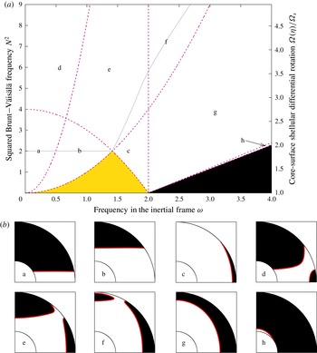
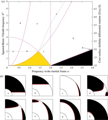
Figure 1 shows the various regions of the parameter space, for axisymmetric modes (
 $m=0$
), for an aspect ratio of the shell
 ${\it\eta}=0.35$
, which is the aspect ratio of the liquid core of the Earth, but also that of the radiative region of a young massive star of approximately 40 solar masses. The yellow domain contains all H modes. There are no gravito-inertial modes in the black area (the elliptic domain covers the whole shell). The white area is for HT modes. We notice that frequency domains accessible to HT modes increase with
 $N^{2}$
and the subsequent differential rotation. As there are regions of the shell rotating faster than the average velocity, gravito-inertial modes can exist with a higher frequency than in the solid-body rotation case. When
 $N^{2}$
is increased, the H-mode domain gets smaller, and there are no H modes at
 $N^{2}>2$
.
The various propagation domains for HT modes are shown in the miniatures. The purple dashed curves mark the transition between the different geometries of the modes, and are obtained by setting
 $m=0$
in (3.6)–(3.9).
We therefore find eight possible HT modes geometries with distinct propagation properties for the characteristics. Remarkably,
-
(i) geometries a and b are similar to the so-called H2 modes of Dintrans et al. (Reference Dintrans, Rieutord and Valdettaro1999), whereas geometries c and g are somewhat reminiscent of their E2 modes,
-
(ii) geometries d, e and f feature two turning surfaces in the shell,
-
(iii) geometries a, d and f feature an acute angle between a turning surface and a boundary of the shell that may lead to the so-called wedge trapping of the modes (Dintrans et al. Reference Dintrans, Rieutord and Valdettaro1999; Gerkema et al. Reference Gerkema, Zimmerman, Maas and van Haren2008).
Domain h is not studied any further due to its small extent in the parameter space, and due to the small extent of the corresponding propagation domain in the shell. Note that, while the borders between the HT-mode geometries generally depend on the shell’s aspect ratio
 ${\it\eta}$
, the boundary of the H-mode region does not.
In figure 1, we have delimited the region of parameter space (located above the grey solid curve), where the waves may be unstable according to criterion (2.14). However, since this criterion is local, this condition is not sufficient.
Finally, we deduce that the frequency range accessible to axisymmetric modes is
 $[0,2{\it\Omega}({\it\eta})]$
, which may be as wide as
 $[0,(1/{\it\Omega}_{s})(2{\it\Omega}_{s}^{2}+N^{2})]$
in our model for the full sphere
 ${\it\eta}=0$
. This range is significantly larger than the predicted range for gravito-inertial modes in a uniformly rotating stratified sphere, which is
 $[0,\sqrt{4{\it\Omega}_{s}^{2}+N^{2}}]$
(Friedlander & Siegmann Reference Friedlander and Siegmann1982a
; Dintrans et al.
Reference Dintrans, Rieutord and Valdettaro1999). Note that our normalization differs from the one used by Friedlander & Siegmann (Reference Friedlander and Siegmann1982a
) and Dintrans et al. (Reference Dintrans, Rieutord and Valdettaro1999) in solid-body rotation: the dimensionless numbers
 $E$
and
 $N^{2}$
differ by a factor of 2, and their
 ${\it\Omega}$
is constant throughout the shell.
(a) Shows a map of the various classes of axisymmetric modes in the
 $({\it\omega},N^{2})$
parameter space, for a shell aspect ratio
 ${\it\eta}=0.35$
. The yellow domain is the H-mode domain (corresponding to modes propagating in the whole shell), whereas the white areas show the HT-mode domains (corresponding to modes propagating in only a part of the shell, and bounded by turning surfaces). The black area corresponds to configurations where no modes exist. Above the solid grey curve, modes are potentially destabilized by the ABCD instability for
 $\mathscr{P}=10^{-5}$
. The dashed purple curves correspond to the apparition of a turning surface at
 $r={\it\eta},r=1$
and
 $\sin ^{2}{\it\theta}=0,1$
and delimit the various HT-mode propagation regions. For each subdomain, a letter indicates the geometry shown in (b), where the domain in which waves may propagate is in white and the evanescent region is in black. The red line is the
 ${\it\Delta}=0$
turning surface on which characteristics bounce.
3.2.2 Non-axisymmetric modes
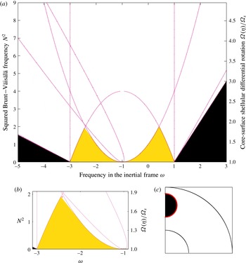
For non-axisymmetric modes with positive
 $m$
, the accessible frequencies are grouped around
 ${\it\omega}=-m$
. The range is no longer symmetrical: the accessible frequency domain extends to frequencies below
 $-m$
, as H modes progressively become HT modes as
 $m$
increases. This can be seen by comparing the top panels of figures 2 and 3. From
 $m$
larger than two, the H-mode domain for
 ${\it\omega}>-m$
also becomes smaller as
 $m$
increases. We find that the frequency range accessible to HT modes with
 $m\geqslant 2$
is
 $[-(m+2){\it\Omega}({\it\eta}):-m{\it\Omega}_{s}+\max (2{\it\Omega}_{s},N)]$
. As
 $\max (2{\it\Omega}_{s},N)$
does not depend on
 $m$
, we note that the extent of the parameter space for prograde modes is constant while the parameter space for retrograde modes increases with
 $m$
.
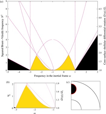
(a) Same as figure 1 but for
 $m=1$
. (b) Extent of the H-mode domain (yellow) for
 $m=1$
retrograde modes. The purple curves mark the expected transition between H and HT modes (white). (c) Elliptic and hyperbolic domains across the shell for a mode at
 $m=1,N^{2}=1.9,{\it\omega}=-2.42$
, indicated by a red tick on the left plot.
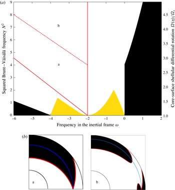
(a) Graph shows the occurrence of corotation resonances as a function of
 ${\it\omega}$
(x-axis) and
 $N^{2}$
(y-axis), for a shell of aspect ratio
 ${\it\eta}=0.35$
and azimuthal wavenumber
 $m=2$
. The yellow domain is the H-mode domain, whereas the white area is the HT-mode domain. The black area corresponds to configurations where no modes exist. Corotation resonances appear in the star for configurations between the two red solid lines. The dashed line separates modes where the critical layer is wholly included in the elliptic part of the shell (subdomain a) and modes where the critical layer cuts through the hyperbolical domain (subdomain b). (b) Shows how the corotation resonance (marked by the solid blue line) may cross the hyperbolic domain (white area). The black area is the elliptic domain and the red lines the turning surfaces.
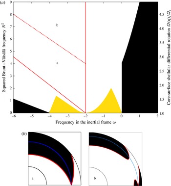
3.2.3 Other turning surfaces
The foregoing results show that the turning surfaces are not simple, leading to numerous configurations for the hyperbolic domain. As warned above, our method for solving equation (3.5) captures only part of the whole set of solutions. Some turning surfaces cannot be calculated from the set of equations (3.6)–(3.9). For our rotation profile, we note that elliptic domains can show up around part of the rotation axis with the pole and the core still in the hyperbolic domain. This is illustrated in figure 2(b,c), which show the distribution of H and HT modes for
 $m=1$
retrograde modes at low stratification. The small white area enclosed between the H-mode domain (yellow area) and its expected boundaries (purple curves) actually corresponds to HT modes. For these specific HT modes, the turning surface does not encompass one of the ‘corners’ of the shell but appears on the rotation axis. Figure 2(c) illustrates this case. Even though only a small part of the parameter space is concerned, it indicates that the boundaries between H and HT modes may not be determined analytically for more complex rotation profiles.
3.2.4 Corotation resonances
For some non-axisymmetric modes, corotation resonances appear where the Doppler-shifted frequency vanishes, i.e. where
 $\widetilde{{\it\omega}}={\it\omega}+m{\it\Omega}(r)=0$
. This resonance is also called a critical layer.
From equation (2.11), the domain of the parameter space
 $({\it\omega},N^{2})$
where a corotation resonance exists in the shell is such that
 $$\begin{eqnarray}\displaystyle -m\left(1+\frac{N^{2}}{2}(1-{\it\eta}^{2})\right)\leqslant {\it\omega}\leqslant -m. & & \displaystyle\end{eqnarray}$$
We note from (3.10) that the range of frequencies at which corotation resonances exist gets larger as
 $m$
increases. It also increases with
 $N^{2}$
at a given
 $m$
.
For configurations where corotation resonances exist, the corotation radius
 $r_{c}$
is given by
 $$\begin{eqnarray}\displaystyle r_{c}=\sqrt{1+\frac{2}{N^{2}}\left(1+\frac{{\it\omega}}{m}\right)}. & & \displaystyle\end{eqnarray}$$
We need to determine whether the corotation radius intersects the hyperbolic domain, that is, if
 ${\it\Delta}(r_{c})>0$
. Setting
 $r=r_{c}$
and
 $\widetilde{{\it\omega}}=0$
in (3.4), we find that
 ${\it\Delta}(r_{c})$
is positive if and only if
 $Nr_{c}>2$
, that is, using (2.11), if
 $$\begin{eqnarray}\displaystyle {\it\omega}>m\left(1-\frac{N^{2}}{2}\right). & & \displaystyle\end{eqnarray}$$
Figure 3 shows the parameter range in the
 $({\it\omega},N^{2})$
plane where corotation resonances exist in the shell for
 $m=2$
. The domain where critical layers exist in the shell is enclosed between the two solid lines. We note that corotation resonances only exist for HT modes, as
 $\widetilde{{\it\omega}}=0$
implies
 ${\it\Delta}=0$
at the equator in (3.5). We find that the parameter domain for modes exhibiting corotation resonances gets larger when
 $m$
increases, and most of the modes in the
 ${\it\omega}<-m$
domain exhibit corotation resonances.
We distinguish two possibilities, depending on whether (3.12) is satisfied or not. If
 ${\it\omega}$
satisfies (3.10) but not (3.12), the corotation radius is inside the elliptic domain, in which modes do not propagate, and the interaction between the corotation resonance and the modes is likely small. Since
 $\widetilde{{\it\omega}}=0$
and
 $z=0$
in (3.4) implies
 ${\it\Delta}=0$
, we find that the turning surface and the corotation radius intersect each other in the equatorial plane only. In figure 3(a), this happens in the subdomain a below the dashed line. A meridional cut of a mode in subdomain a is shown in the first plot of figure 3(b), where the critical layer is denoted by a blue line.
Conversely, if (3.10) and (3.12) are both satisfied, the corotation resonance goes through the hyperbolic domain and is expected to influence the propagation of the waves and the associated characteristics either by introducing nonlinear effects or by limiting the propagation domain. This corresponds to subdomain b in figure 3(a), from the dashed line upwards. The corresponding second plot in figure 3(b) shows an example of such a mode where the critical layer (blue line) crosses the hyperbolical domain (white area). For this case, the calculation leading to (3.12) also shows that the intersection between the hyperbolic domain and the corotation surface is located at latitudes
 ${\it\vartheta}$
satisfying
 $$\begin{eqnarray}\displaystyle \sin {\it\vartheta}<\frac{2}{Nr_{c}}. & & \displaystyle\end{eqnarray}$$
As we expect the critical layer to have an effect on the damping or excitation of the mode (e.g. Rieutord et al. Reference Rieutord, Triana, Zimmerman and Lathrop2012), the ability of the wave to cross this layer needs to be investigated. This is done by computing the phase and group velocities (see below), and by solving the fully dissipative problem (§ 4).
3.3 Dispersion relation, phase and group velocities
Further insight into the propagation properties of gravito-inertial waves over a shellular differential rotation may be obtained through the dispersion relation of the waves.
To determine the interplay between paths of characteristics and corotation resonances, we derive from (3.1) the following dispersion relation
 $$\begin{eqnarray}\displaystyle \widetilde{{\it\omega}}^{2}=\frac{\mathscr{B}^{2}}{k^{2}}\quad \text{with}~\mathscr{B}=[N^{2}(k_{s}z-k_{z}s)^{2}+k_{z}^{2}A_{s}-k_{s}k_{z}A_{z}]^{1/2}, & & \displaystyle\end{eqnarray}$$
where
 $\boldsymbol{k}=k_{s}\boldsymbol{e}_{s}+k_{z}\boldsymbol{e}_{z}$
is the wavevector,
 $k=\Vert \boldsymbol{k}\Vert =\sqrt{k_{s}^{2}+k_{z}^{2}}$
. Equation (3.14) reduces to (A.7) of Baruteau & Rieutord (Reference Baruteau and Rieutord2013) in the case with no stratification
 $(N^{2}=0)$
.
This equation yields the phase and group velocities in the corotating frame,
 $\boldsymbol{v}_{p}$
and
 $\boldsymbol{v}_{g}$
respectively,
 $$\begin{eqnarray}\displaystyle \boldsymbol{v}_{p}=\pm \frac{\mathscr{B}\boldsymbol{k}}{k^{3}}, & & \displaystyle\end{eqnarray}$$
and
 $$\begin{eqnarray}\displaystyle \boldsymbol{v}_{g}=\pm \frac{1}{k^{3}}\left[\left(k^{2}\frac{\text{d}\mathscr{B}}{\text{d}k_{s}}-k_{s}\mathscr{B}\right)\boldsymbol{e}_{s}+\left(k^{2}\frac{\text{d}\mathscr{B}}{\text{d}k_{z}}-k_{z}\mathscr{B}\right)\boldsymbol{e}_{z}\right]. & & \displaystyle\end{eqnarray}$$
The dispersion relation indicates the behaviour of a wave near the corotation radius. Upon approaching the corotation resonance,
 $\widetilde{{\it\omega}}\rightarrow 0$
which implies that either
 $k\rightarrow \infty$
or
 $\mathscr{B}\rightarrow 0$
.
-
(i) If
$k\rightarrow \infty$
at finite
$k_{z}$
, then
$\boldsymbol{v}_{p}=0$
and
$\boldsymbol{v}_{g}=0$
, the gravito-inertial waves do not cross the corotation radius. If corotation is in the elliptic domain but touches the turning surface on the equator
$z=0$
, then the characteristics become more and more vertical (namely parallel to the rotation axis) as they approach the corotation, but the corotation is never reached. The wave is likely dissipated there. -
(ii) If
$\mathscr{B}\rightarrow 0$
, then
$\boldsymbol{v}_{p}\rightarrow 0$
and
$\boldsymbol{v}_{g}\neq 0$
in the general case. In this situation, the waves can go through the corotation resonance in the hyperbolic domain, but nonlinear effects are expected (Barker & Ogilvie Reference Barker and Ogilvie2010).


We only see the occurrence of this second possibility in our simulations (§ 4): as shown in figure 11, the eigenmodes we compute are able to cross the corotation radius.
3.4 Critical latitudes
Critical latitudes are another type of singularity that may affect waves in a spherical shell (e.g. Rieutord et al. Reference Rieutord, Georgeot and Valdettaro2001). As with all singularities, they generate dissipative structures, and are thus important to understanding the dynamics of tidally interacting bodies (Goodman & Lackner Reference Goodman and Lackner2009; Ogilvie Reference Ogilvie2009; Rieutord & Valdettaro Reference Rieutord and Valdettaro2010; Favier et al. Reference Favier, Barker, Baruteau and Ogilvie2014).
A critical latitude is a latitude
 ${\it\vartheta}$
on the bounding spheres where the characteristics are tangent to the boundary. They appear when
 $|\widetilde{{\it\omega}}(r)|\leqslant 2{\it\Omega}(r)$
, that is
 $$\begin{eqnarray}\displaystyle \sin {\it\vartheta}=\frac{\widetilde{{\it\omega}}(r)}{2{\it\Omega}(r)},\quad \text{with}~r={\it\eta}~\text{or}~r=1. & & \displaystyle\end{eqnarray}$$
The inner and outer critical latitudes,
 ${\it\theta}_{i}$
and
 ${\it\theta}_{o}$
, are given by
 $$\begin{eqnarray}\displaystyle \sin {\it\vartheta}_{o}=\frac{{\it\omega}+m}{2},\quad \sin {\it\vartheta}_{i}=\frac{{\it\omega}}{2{\it\Omega}({\it\eta})}+\frac{m}{2}. & & \displaystyle\end{eqnarray}$$
There is a critical latitude on the inner boundary if
 $0<\sin {\it\vartheta}_{i}<1$
, that is when
 $$\begin{eqnarray}\displaystyle -m{\it\Omega}({\it\eta})<{\it\omega}<(-m+2){\it\Omega}({\it\eta}), & & \displaystyle\end{eqnarray}$$
and similarly, there is a critical latitude on the outer boundary if
 $$\begin{eqnarray}\displaystyle -m<{\it\omega}<-m+2. & & \displaystyle\end{eqnarray}$$
In the frequency ranges where critical latitudes exist, some modes may be associated with shear layers emitted at these latitudes (Rieutord & Valdettaro Reference Rieutord and Valdettaro2010). While it is not necessarily the case for free modes of oscillations, tidally forced flows in a spherical shell seem to always excite the shear layers associated with the inner critical latitudes when they exist (as shown by Goodman & Lackner Reference Goodman and Lackner2009; Ogilvie Reference Ogilvie2009). For other geometries, concave critical latitudes may be excited (see, e.g. Swart et al. Reference Swart, Manders, Harlander and Maas2010).
3.5 Lyapunov exponents
The paths of characteristics computed using equations (3.2)–(3.3) often tend towards a short-period limit cycle, known as an attractor. When such a structure exists, the kinetic energy of an eigenmode is generally concentrated around the attractor. These modes are expected to be strongly damped due to the singular nature of the attractor at vanishing viscosities. It is therefore of interest to assess the presence and the strength of the focusing towards attractors, and for this we compute the Lyapunov exponent of the characteristic trajectories. It quantifies whether characteristics get closer to each other after multiple reflections onto the boundaries of the hyperbolic domain. Since our problem can be studied in a meridional quarter-plane of the shell, we can conveniently use the rebounds on the rotational and equatorial axes. From the distance between two consecutive rebounds on the rotation axis, or on the equatorial plane,
 ${\it\delta}s_{k}$
or
 ${\it\delta}z_{k}$
respectively, we derive the two following Lyapunov exponents,
 ${\it\Lambda}_{s}$
or
 ${\it\Lambda}_{z}$
respectively:
 $$\begin{eqnarray}\displaystyle {\it\Lambda}_{s}=\lim _{N_{s}\rightarrow \infty }\frac{1}{N_{s}}\mathop{\sum }_{k=1}^{N_{s}}\ln \left|\frac{{\it\delta}s_{k+1}}{{\it\delta}s_{k}}\right|\quad \text{and}\quad {\it\Lambda}_{z}=\lim _{N_{z}\rightarrow \infty }\frac{1}{N_{z}}\mathop{\sum }_{k=1}^{N_{z}}\ln \left|\frac{{\it\delta}z_{k+1}}{{\it\delta}z_{k}}\right|. & & \displaystyle\end{eqnarray}$$
There are some instances where an attractor may feature more than one rebound on a given axis where the Lyapunov exponent is computed. When that happens, our numerical procedure finds the coordinate of each convergence point and computes the exponent selecting the rebounds that tend towards that convergence point.
Formally, Lyapunov exponents on both axes should have the same value. We compute the Lyapunov exponents with several pairs of characteristics starting in various parts of the shell. Since this calculation is sometimes difficult numerically, we use the average value of
 ${\it\Lambda}_{s}$
and
 ${\it\Lambda}_{z}$
to derive the Lyapunov exponent.
A negative Lyapunov exponent means that the two characteristics get closer to each other, and end up converging towards an attractor. The more negative the exponent, the faster the convergence.
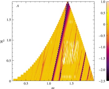
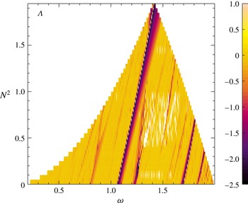
Lyapunov exponent for H modes for
 ${\it\eta}=0.35$
. The dark ridges are modes focused on a short-period attractor.
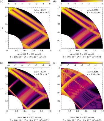
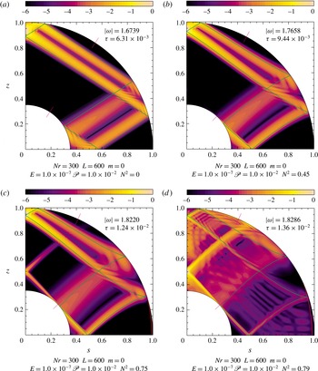
Meridional slices of kinetic energy (normalised to its maximum value, in logarithmic scale) obtained by solving the dissipative linearised hydrodynamics equations, with attractors (green) and turning surfaces (red) overplotted. The pink ticks at the inner and outer borders denote the critical latitudes. From (a–d), the Brunt–Väisälä frequency is increased for the same mode (
 ${\it\eta}=0.35,E=10^{-7},\mathscr{P}=10^{-2}$
, starting from
 ${\it\omega}=1.67,N^{2}=0$
). The mode is distorted until the structure is suddenly changed when the shear layer crosses the critical latitude (see main text).
In figure 4, we show the Lyapunov exponent in the
 $({\it\omega},N^{2})$
plane, for axisymmetric H modes. We see ridges where the Lyapunov exponent is very negative, which implies the presence of a strong attractor in the shell. Each ridge of negative Lyapunov exponent consists of the same attractor progressively distorted by the differential rotation: as
 $N^{2}$
and the subsequent differential rotation increase, the frequency varies but the overall shape of the attractor is conserved, as will be illustrated in figure 5. We note that the strength of the focussing for a given attractor is constant: the Lyapunov exponent is constant along a ridge of negative value. These modes are expected to be strongly damped by dissipative processes. However, most of the
 $({\it\omega},N^{2})$
plane corresponds to long-period attractors compatible with low dissipation, and these modes are therefore more prone to yield observable stellar pulsations. We note that by taking a horizontal slice in figure 4 at
 $N^{2}=0$
, we retrieve the Lyapunov exponents computed for inertial modes in a solid-body rotating shell by Rieutord, Georgeot & Valdettaro (Reference Rieutord, Georgeot and Valdettaro2000), Rieutord et al. (Reference Rieutord, Georgeot and Valdettaro2001).
For non-negative values of the Lyapunov exponent, there is no convergence towards a limit cycle. Because the sums in equation (3.21a,b ) could not necessarily be carried out with as many iterations as formally required, they do not cancel out. For some values (white regions inside the graph), the computation has not converged, but the Lyapunov exponents are likely very small in absolute value.
As will be shown in § 4, the kinetic energy of eigenmodes is not necessarily distributed along the predicted attractor: other kinds of singularities like the critical latitude singularity or corotation resonances may also affect the kinetic energy distribution. Due to turning surfaces, computing the Lyapunov exponents of HT modes (whether they are focused on a short-period attractor or in a wedge) is much more difficult, and no significant map could be computed.
4 Dissipative problem
After the foregoing study of the properties of the eigenmodes in the non-dissipative limit, we now investigate the role of dissipative processes on the structure and damping (or growth) rates of gravito-inertial modes. In this section we describe the numerical method we used, show representative examples of axisymmetric and non-axisymmetric modes and discuss the physical implication of the results.
4.1 Numerical method
In order to study the full dissipative eigenvalue problem, that consists of equations (2.7) to (2.9) with related boundary conditions, we now solve the problem numerically using a spectral method similar to that used in Baruteau & Rieutord (Reference Baruteau and Rieutord2013). Equations are projected onto spherical harmonics (see Rieutord Reference Rieutord1987), expanding the velocity and temperature perturbations as
 $$\begin{eqnarray}\displaystyle \boldsymbol{v}(r,{\it\theta},{\it\phi})=\mathop{\sum }_{\ell =0}^{\infty }\mathop{\sum }_{m=-\ell }^{\ell }u_{m}^{\ell }(r)\boldsymbol{R}_{\ell }^{m}+v_{m}^{\ell }(r)\boldsymbol{S}_{\ell }^{m}+w_{m}^{\ell }(r)\boldsymbol{T}_{\ell }^{m},\quad T=\mathop{\sum }_{\ell =0}^{\infty }\mathop{\sum }_{m=-\ell }^{\ell }t_{m}^{\ell }Y_{\ell }^{m}, & & \displaystyle \nonumber\\ \displaystyle & & \displaystyle\end{eqnarray}$$
where
 $\boldsymbol{R}_{\ell }^{m}=Y_{\ell }^{m}({\it\theta},{\it\phi})\boldsymbol{e}_{r},\boldsymbol{S}_{\ell }^{m}=\boldsymbol{{\rm\nabla}}Y_{\ell }^{m}({\it\theta},{\it\phi}),\boldsymbol{T}_{\ell }^{m}=\boldsymbol{{\rm\nabla}}\times Y_{\ell }^{m}({\it\theta},{\it\phi})$
and where
 $Y_{\ell }^{m}$
denotes the normalized spherical harmonics. In the radial direction, equations are discretised on the Gauss–Lobatto grid associated with Chebyshev polynomials. The equations are truncated at order
 $L$
in the spherical harmonics expansion and at order
 $N_{r}$
on the Chebyshev grid. Appropriate values of
 $N_{r},L$
depend on the mode properties and the Ekman and Prandtl numbers. We use the Arnoldi–Chebyshev algorithm to compute eigenvalues
 ${\it\omega}$
and their associated eigenvectors. This method allows us to find the frequencies corresponding to the least-damped modes around a given initial guess. By changing slightly the guess, we can test for round-off errors (for more details on the numerical method, see Valdettaro et al.
Reference Valdettaro, Rieutord, Braconnier and Fraysse2007). All modes are computed assuming symmetry with respect to the equatorial plane, and using stress-free boundary conditions at both the inner and outer radial boundaries of the shell.
Projecting the momentum equation (2.7) on
 $\boldsymbol{R}_{\ell }^{m}$
and
 $\boldsymbol{T}_{\ell }^{m}$
and the heat equation (2.9) on
 $Y_{\ell }^{m}$
we obtain
 $$\begin{eqnarray}\displaystyle & & \displaystyle E{\it\Delta}_{\ell }w_{m}^{\ell }+\left[\frac{2\text{i}m{\it\Omega}}{\ell (\ell +1)}-\text{i}\widetilde{{\it\omega}}\right]w_{m}^{\ell }\nonumber\\ \displaystyle & & \displaystyle \quad =-2{\it\Omega}[A(\ell ,m)r^{\ell -1}\partial _{r}(r^{-\ell +2}u_{m}^{\ell -1})+A(\ell +1,m)r^{-\ell -2}\partial _{r}(r^{\ell +3}u_{m}^{\ell +1})]\nonumber\\ \displaystyle & & \displaystyle \qquad +\,r\partial _{r}{\it\Omega}[-(\ell +1)A(\ell +1,m)u_{m}^{\ell +1}+\ell A(\ell ,m)u_{m}^{\ell -1}],\end{eqnarray}$$
 $$\begin{eqnarray}\displaystyle & & \displaystyle E{\it\Delta}_{\ell }{\it\Delta}_{\ell }(ru_{m}^{\ell })+\left[\frac{2\text{i}m{\it\Omega}}{\ell (\ell +1)}-\text{i}\widetilde{{\it\omega}}\right]{\it\Delta}_{\ell }(ru_{m}^{\ell })=-2\text{i}m\partial _{r}{\it\Omega}\left(u_{m}^{\ell }+v_{m}^{\ell }\right)-\text{i}mr\partial _{rr}^{2}{\it\Omega}u_{m}^{\ell }\nonumber\\ \displaystyle & & \displaystyle \qquad +\,2{\it\Omega}\left[B(\ell ,m)r^{\ell -1}\partial _{r}\left(r^{1-\ell }w_{m}^{\ell -1}\right)+B(\ell +1,m)r^{-\ell -2}\partial _{r}(r^{\ell +2}w_{m}^{\ell +1})\right]\nonumber\\ \displaystyle & & \displaystyle \qquad +\,2\partial _{r}{\it\Omega}\left[B(\ell ,m)w_{m}^{\ell -1}+B(\ell +1,m)w_{m}^{\ell +1}\right]-N^{2}\ell (\ell +1)t_{m}^{\ell },\end{eqnarray}$$
 $$\begin{eqnarray}\displaystyle \text{i}\widetilde{{\it\omega}}t_{m}^{\ell }-ru_{m}^{\ell }=\frac{E}{\mathscr{P}}{\it\Delta}_{\ell }t_{m}^{\ell }, & & \displaystyle\end{eqnarray}$$
where we defined
 $$\begin{eqnarray}\displaystyle {\it\Delta}_{\ell }=\frac{\text{d}^{2}}{\text{d}r^{2}}+\frac{2}{r}\frac{\text{d}}{\text{d}r}-\frac{\ell (\ell +1)}{r^{2}}, & & \displaystyle\end{eqnarray}$$
 $$\begin{eqnarray}\displaystyle A(\ell ,m)=\frac{1}{\ell ^{2}}\left(\frac{\ell ^{2}-m^{2}}{4\ell ^{2}-1}\right)^{1/2},\quad B(\ell ,m)=\ell ^{2}(\ell ^{2}-1)A(\ell ,m). & & \displaystyle\end{eqnarray}$$
In equations (4.2)–(4.3), we used mass conservation (2.8) which yields
 $$\begin{eqnarray}\displaystyle v_{m}^{\ell }=\frac{1}{\ell (\ell +1)r}\frac{\partial r^{2}u_{m}^{\ell }}{\partial r}. & & \displaystyle\end{eqnarray}$$
Setting to zero the stratification and the subsequent differential rotation, these equations reduce to equations (2.2) of Rieutord & Valdettaro (Reference Rieutord and Valdettaro1997) for inertial modes in solid-body rotation. Removing only stratification, these equations reduce to equations (4.2) of Baruteau & Rieutord (Reference Baruteau and Rieutord2013). Finally, taking only stratification into account without differential rotation, this set of equations reduces to equations (2.5) of Dintrans et al. (Reference Dintrans, Rieutord and Valdettaro1999) for gravito-inertial modes.
4.2 Axisymmetric modes: illustrative cases
Let us first describe a few axisymmetric (
 $m=0$
) modes obtained for various stratifications and associated differential rotations. We illustrate the various geometries for H and HT modes by comparing the solutions to the fully dissipative equations with their non-dissipative counterparts. For all the modes that we have calculated, we show a meridional slice of kinetic energy, normalized at its maximum value, in a quarter-plane. We recall that all computed modes are symmetric with respect to the equatorial plane.
As a first illustration of the impact of the stratification and the associated differential rotation, we follow a pure inertial mode while increasing the Brunt–Väisälä frequency. To do so, we increase
 $N^{2}$
by small increments using the eigenfrequency obtained for a given mode as an initial guess for the next computed mode. Figure 5 shows the kinetic energy in a meridional plane for increasing values of the Brunt–Väisälä frequency at the surface of the shell. We recall that as the surface Brunt–Väisälä frequency increases, so do the linear Brunt–Väisälä frequency gradient and the rate of shellular differential rotation. In (a–d), we find a singular shear layer that closely follows an attractor of characteristics (in green).
The (a) is for
 $N^{2}=0$
and thus solid-body rotation. The characteristics and the shear layers then follow straight lines in the shell. The (b) (
 $N^{2}=0.45$
) shows the distortion induced by the stratification and the consequent differential rotation: the characteristics are now curved, even though the overall shape of the attractor is conserved. By increasing the stratification further ((c),
 $N^{2}=0.75$
), the critical latitude singularity at the inner core gets excited. Owing to the fluid’s viscosity, part of the energy is then focused on the shear layer tangent to the core. The mode has now changed to a HT mode, as a turning surface appears near the equator (shown by a red curve in the panels). As shown in (d), when increasing the stratification even further (
 $N^{2}=0.79$
), the shear layer emitted at the critical latitude singularity dominates the kinetic energy distribution inside the shell.
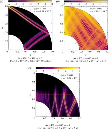
Meridional slices of kinetic energy for a sample of modes (relative to maximum, in log scale). Attractors (green), turning surfaces (red) and critical latitudes (pink ticks) overplotted. The various geometries are discussed in the main text.
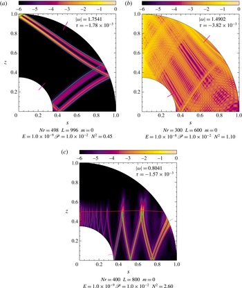
Figure 6 illustrates the diversity of the H and HT modes predicted in our model. Two H modes are shown in (a,b). The mode displayed in (a) is obtained by a follow-up of the mode displayed in figure 5(b) by lowering the Ekman number. The energy is neatly focused on a shear layer whose location is well described by the associated attractor. The mode in (b) is associated with a quasi-periodic trajectory of characteristics. The kinetic energy is distributed nearly uniformly over the whole shell. The mode in figure 6(c) is a HT mode, which belongs to subdomain b in figure 1. The predicted turning surface (red curve) nicely delimits the propagation domain, even though the kinetic energy penetrates somehow in the evanescent region. The extent of the eigenfunction in the elliptic domain is directly related to the diffusion coefficients
 ${\it\nu}$
and
 ${\it\kappa}$
. Attractors matching the shear layers (green curves) are obtained from characteristics spanning the propagation domain and bouncing on the turning surface. This mode simultaneously focusses most of its energy on an attractor and excites the critical latitude singularity, letting a small fraction of its energy propagating towards the rotation axis. The turning surface may also introduce singularities, such as the so-called wedge trapping, which is displayed in figure 9 and discussed in the next section.
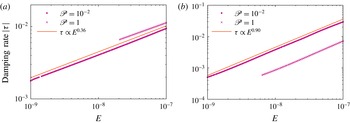
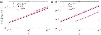
Damping rate as a function of the Ekman number for the H modes displayed in figure 6(a,b). (a) Corresponds to the mode focused on a short-period attractor and (b) to the quasi-periodical mode. The data points are obtained by following a given mode with decreasing the Ekman number, for two different values of the Prandtl number:
 $10^{-2}$
(filled circles) and
 $1$
(crosses), while the solid line is the best fit trend at
 $E\rightarrow 0$
.
4.3 Axisymmetric modes: dissipative properties
We examine in this section the dissipative properties of axisymmetric modes with shellular rotation resulting from the stratification. Because of the very small values of the Ekman and Prandtl numbers in stars or planets, we are interested in the asymptotic behaviour of the modes and their eigenfrequency when
 $E$
and
 $\mathscr{P}$
vanish (but verifying the constraint
 $E\ll \mathscr{P}$
). As astrophysical parameters are beyond reach, we first try to infer asymptotic scaling laws of damping rates for various modes.
Figure 7 shows the damping rate
 $|{\it\tau}|$
as a function of the Ekman number for two H modes at two different Prandtl numbers. In (a,b),
 $E$
decreases from
 $10^{-7}$
to
 $10^{-9}$
for
 $\mathscr{P}=1$
and
 $\mathscr{P}=10^{-2}$
. Figure 7(a) corresponds to the H mode in figure 6(a), which is focused around a short-period attractor. We find that the decrease of
 $|{\it\tau}|$
is well reproduced by
 $E^{0.36}$
. This dependency on the Ekman number is reminiscent of the scaling laws obtained by Rieutord et al. (Reference Rieutord, Georgeot and Valdettaro2001) for inertial modes focussed on short-period attractors. For these modes, the expected scalings are
 $|{\it\tau}|\propto E^{{\it\alpha}}$
when
 $E\rightarrow 0$
, with
 ${\it\alpha}\in [1/3,1/2]$
. Figure 7(b) corresponds to the quasiperiodic H-mode in figure 6(b). We find the scaling of
 $|{\it\tau}|\propto E^{0.9}$
for both Prandtl numbers.
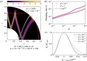
(a) Kinetic energy for a HT mode featuring two turning surfaces, at
 ${\it\omega}=1.39,{\it\eta}=0.35,E=10^{-9},\mathscr{P}=1$
and
 $N^{2}=3$
(relative to maximum, in log scale). (b) Damping rate as a function of the Ekman number. The data points are obtained by following the mode with decreasing the Ekman number, for two different values of the Prandtl number:
 $10^{-2}$
(filled circles) and
 $1$
(triangles), while the solid line is the best fit trend at
 $E\rightarrow 0$
. (c) Width of the shear layer over four decades in the Ekman number, rescaled by the best fit obtained.
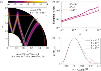
Figure 8 shows the same follow-up calculation for an HT mode with two turning surfaces and a short-period attractor. Figure 8(b) shows the evolution of the damping rate
 $|{\it\tau}|$
when decreasing the Ekman number from
 $10^{-6}$
to
 $10^{-9}$
, at
 $\mathscr{P}=10^{-2}$
and
 $1$
. We find that
 $|{\it\tau}|$
approximately scales with
 $E^{0.47}$
at low
 $E$
and constant
 $\mathscr{P}$
. Similarly, we follow this mode decreasing
 $\mathscr{P}$
from
 $1$
to
 $10^{-3}$
at
 $E=10^{-7}$
(not shown here), and find
 $|{\it\tau}|\propto \mathscr{P}^{-0.5}$
at low
 $\mathscr{P}$
at constant
 $E$
. We also measure the width of the shear layer while decreasing
 $E$
, and find that the width of the shear layer scales with
 $E^{0.22}$
at fixed
 $\mathscr{P}$
. This is illustrated in figure 8(c), where the kinetic energy profiles in the shear layer at various Ekman number values, once rescaled by
 $E^{0.22}$
, overlap neatly (this plot is similar to that of figure 13(b) in Dintrans et al.
Reference Dintrans, Rieutord and Valdettaro1999). The obtained scaling is reminiscent of the
 $E^{1/4}-$
scaling derived for the shear layer width by Dintrans et al. (Reference Dintrans, Rieutord and Valdettaro1999).
(a) Kinetic energy for a HT mode in which a wedge trapping occurs, at
 ${\it\omega}=0.33,{\it\eta}=0.35,E=10^{-10},\mathscr{P}=10^{-2}$
and
 $N^{2}=6.7$
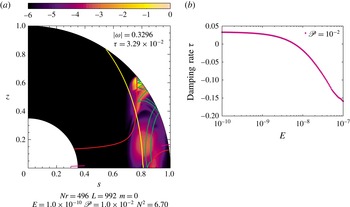
(relative to maximum, in log scale). The turning surfaces are shown in red and the characteristics in green, while the area outside the yellow curve is ABCD-unstable (see § 2.4). (b) Damping rate as a function of the Ekman number. The data points are obtained by following a mode with decreasing the Ekman number, the solid line is the best fit trend at
 $E\rightarrow 0$
.
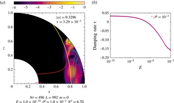
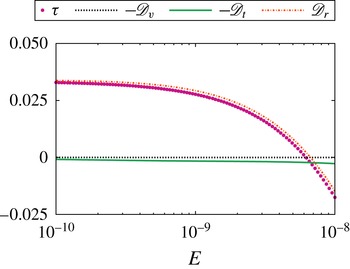
Figure 9(a) shows a HT mode with two turning surfaces bounding the hyperbolic domain, corresponding to the subdomain d of figure 1. As alluded to at the end of § 4.2, the turning surfaces and the outer surface of the shell form an acute angle in which the kinetic energy is focused. This focussing, known as wedge trapping, is also described by the characteristics which show that rays should converge towards the intersection between the shell’s surface and the higher-latitude turning surface. Our calculation confirms that most of the modes kinetic energy is indeed confined in that location. Wedge trapping is possible in subdomains a, d and f of figure 1. Figure 9(b) shows that, when decreasing the Ekman number, this mode becomes unstable and its growth rate becomes independent of
 $E$
. The critical Ekman number below which instability sets in is
 $E_{c}\sim 7\times 10^{-9}$
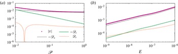
. Most probably, this destabilization is due to the ABCD instability. Indeed, the part of the shell where the local ABCD instability criterion (2.14) is satisfied corresponds to the place occupied by the eigenfunction (see figure 9). The border of the ABCD-unstable domain is only slightly changed around the equator when considering astrophysically relevant Prandtl numbers such as
 $\mathscr{P}=10^{-5}$
. To be complete, the other possible driving of the instability, namely the shear instability (see criterion (2.21)) is only satisfied along the inner boundary (at
 ${\it\theta}>40^{\circ }$
,
 $r<0.45$
) and can thus be eliminated. We give further insight on the driving of the instability in § 4.5.
Kinetic energy for a HT mode at
 ${\it\omega}=0.25$
,
 ${\it\eta}=0.35$
,
 $E=10^{-10},\mathscr{P}=10^{-2}$
and
 $N^{2}=1.5$
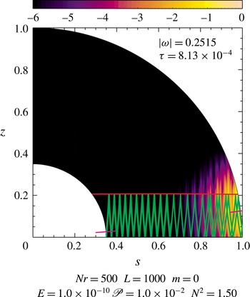
(relative to maximum, in log scale). For this mode, a wedge trapping is possible, but does not occur (see main text). The turning surface (red curve), the path of characteristic (green curve) and the critical latitudes (pink ticks) are overplotted.
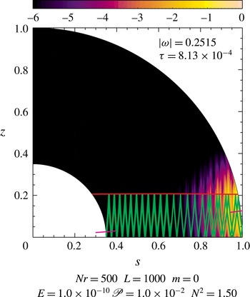
In figure 10, we show another mode in which a wedge is formed at the inner boundary. We notice that the kinetic energy is not focused in the wedge. This is due to the presence of the critical latitude singularity: characteristics hitting the core at latitudes
 ${\it\theta}>{\it\theta}_{c}$
converge towards the wedge in a singular point, while characteristics hitting the core at
 ${\it\theta}<{\it\theta}_{c}$
form a periodic limit cycle. When this dichotomy appears, the kinetic energy seems to be always focussed on the periodic attractor, and the presence of a wedge does not impact the shape of the eigenmode.
4.4 Non-axisymmetric modes: illustrative cases
To complete the foregoing picture given by axisymmetric modes, we now focus on non-axisymmetric ones, emphasizing the differences introduced by a non-zero azimuthal wavenumber
 $m$
. As explained in § 3.2, the main feature of non-axisymmetric modes is the presence of corotation resonances, where the Doppler-shifted frequency vanishes, that is places where
 ${\it\omega}+m{\it\Omega}(r)=0$
.
4.4.1 Corotation resonances
We have seen in § 3.2.4 the conditions for a corotation resonance (or a critical layer) to occur in the spherical shell, its location is given by (3.11). Either the corotation resonance threads the hyperbolic domain, in which case we expect the resonance to have a significant impact on the dissipation properties of the mode, or it stays in the elliptic domain, in which case its impact on the modes dissipation should be marginal.
(a) Kinetic energy for a HT mode exhibiting a corotation resonance in the hyperbolical domain, at
 ${\it\omega}=-3.86,m=3,{\it\eta}=0.35,E=10^{-7},\mathscr{P}=1$
and
 $N^{2}=6$
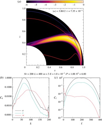
(relative to maximum, in log scale). This mode belongs to subdomain b in figure 3. (b,c) Spectral decomposition on the Chebyshev (b) and the spherical harmonics (c) bases.
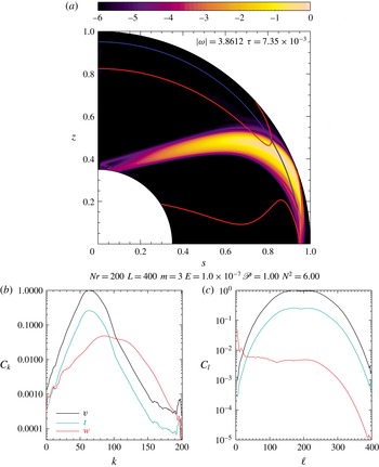
An example of the former case is shown in figure 11(a). We see that the energy is mostly focused on a structure tangent to the corotation layer (blue radius), between the three turning surfaces (red curves). To avoid round-off errors, we had to use a moderate resolution. To reach spectral convergence with this resolution (as shown in (b,c)), we also had to use a relatively high Ekman number. Many of these modes appear to be unstable, though we were not able to follow any of these modes in a wide range of parameters
 $E$
and
 $\mathscr{P}$
, owing to constraints from spatial resolution. The mode shown in figure 11 is unstable. Its positive growth rate can be explained either by the baroclinic instability or by a shear instability, but this latter possibility can actually be excluded: the local instability criterion (2.21) is only met in two small areas around the inner shell (
 ${\it\theta}>40^{\circ },r<0.45$
) and on the equator (
 ${\it\theta}>65^{\circ }$
,
 $r>0.97$
). The non-axisymmetric baroclinic instability criterion (2.18) is met in most of the shell (
 $z>1/6$
), and is likely at the origin of the positive growth rate. As mentioned in § 3.2.4, these corotations are expected to trigger non-linear effects (see Maslowe Reference Maslowe1986).
When the corotation resonance is wholly included in the elliptic part of the shell, we were not able to compute any mode: a satisfactory trade-off between spectral convergence and round-off errors could not be reached (because a high resolution, needed to describe this type of modes accurately, increases dramatically the condition number of the matrices, and therefore the round-off errors).
4.4.2 Regular modes
The eigenvalue problem that we solve is also expected to have some regular or quasi-regular solutions, as found for instance by Dintrans et al. (Reference Dintrans, Rieutord and Valdettaro1999) for solid-body rotation. Such modes are not focused towards any singular shear layer, and are therefore significantly less damped than modes featuring an attractor. Regular modes have a kinetic energy distribution in the shell that is almost independent of the dissipative parameters
 $E$
and
 $\mathscr{P}$
. They may then exist at vanishing viscosity and thermal diffusivity, and are expected to be only weakly damped. As our numerical method can compute the least-damped modes around a given initial frequency guess (see § 4.1), regular modes are expected to be easily found where they exist. Such kind of modes are only found when
 $m\neq 0$
, letting us think that regular or quasi-regular axisymmetric modes do not exist in our set-up.
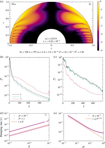
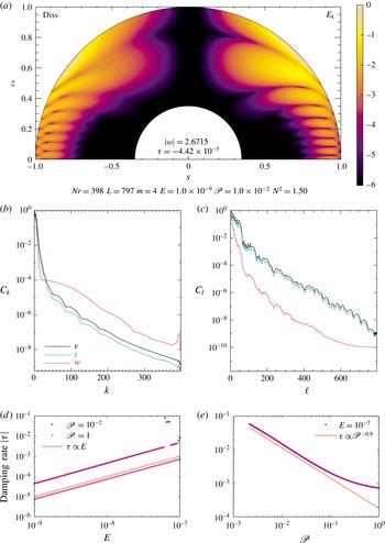
Figure 12 illustrates the properties of such a mode. Here, the spectral convergence is easily reached compared to the previous modes. As (d,e) show, we assess the scaling laws of the damping rate
 $|{\it\tau}|$
with the Ekman number at fixed Prandtl number (that is, while varying viscosity and thermal diffusivity at the same rate) and with
 $\mathscr{P}$
at fixed
 $E$
(that is, varying the thermal diffusivity while keeping the viscosity constant). We find
 $|{\it\tau}|\propto E$
at constant
 $\mathscr{P}$
and low
 $E$
, and
 $|{\it\tau}|\propto \mathscr{P}^{-0.9}$
at constant
 $E$
and low
 $\mathscr{P}$
.
Regular mode, at
 ${\it\omega}=-2.67,m=4,{\it\eta}=0.35,E=10^{-9}$
,
 $\mathscr{P}=10^{-2}$
and
 $N^{2}=1.5$
. (a) Meridional slice of the viscous dissipation (left quarter-panel) and the kinetic energy (right). Both are normalised by their maximum value, and plotted in logarithmic scale. (b,c) Spectral decomposition on the Chebyshev (b) and the spherical harmonics (c) bases. (d,e) Damping rate as a function of the Ekman number for
 $\mathscr{P}=10^{-2}$
and
 $1$
(d), and as a function of the Prandtl number for
 $E=10^{-7}$
(e).
4.5 Interpretation of scaling laws
In the previous section we inspected numerically the behaviour of gravito-inertial modes as the dissipation parameters are varied. Clearly, the damping rates often show a scaling law with either the Ekman number or the Prandtl number, when these parameters tend to small values. We now attempt to interpret these behaviours, however without a detailed boundary layer analysis, which is beyond the scope of this first exploration. We rather resort to the integral expression of the damping rate, which reads
 $$\begin{eqnarray}\displaystyle {\it\tau}=-\mathscr{D}_{v}-\mathscr{D}_{t}+\mathscr{D}_{r}, & & \displaystyle\end{eqnarray}$$
that is, the sum of the viscous and thermal dissipations, and the differential rotation driving. The aforementioned terms of equation (4.8) are given by
 $$\begin{eqnarray}\displaystyle & & \displaystyle \mathscr{D}_{v}=\frac{1}{\mathscr{E}}\frac{E}{2}\displaystyle \int _{V}\unicode[STIX]{x1D634}_{ij}^{2}\,\text{d}V,\quad \mathscr{D}_{t}=\frac{1}{\mathscr{E}}N^{2}\frac{E}{\mathscr{P}}\displaystyle \int _{V}|\boldsymbol{{\rm\nabla}}T|^{2}\,\text{d}V,\quad \mathscr{D}_{r}=\frac{1}{\mathscr{E}}\displaystyle \int _{V}s\mathscr{R}\{v_{r}\partial _{r}{\it\Omega}v_{{\it\phi}}^{\star }\}\,\text{d}V,\nonumber\\ \displaystyle & & \displaystyle\end{eqnarray}$$
where
 $$\begin{eqnarray}\displaystyle \mathscr{E}=\displaystyle \int _{V}\boldsymbol{v}^{2}\,\text{d}V+N^{2}\displaystyle \int _{V}|T|^{2}\,\text{d}V & & \displaystyle\end{eqnarray}$$
and
 $\unicode[STIX]{x1D634}_{ij}$
is the stress tensor, while
 $\mathscr{R}\{z\}$
and
 $z^{\star }$
designate the real part and the complex conjugate of
 $z$
, respectively. We follow the method detailed in appendix B of Dintrans et al. (Reference Dintrans, Rieutord and Valdettaro1999) to derive equations (4.8) and (4.9). It is clear that
 $\mathscr{D}_{r}$
is the only term that can contribute positively to the growth rate, and explain unstable gravito-inertial modes.
We compute the expected damping rates from the velocity and temperature fields obtained in our simulations, through (4.8). Provided the mode computation is accurately converged, the expected damping rate matches the computed eigenvalue. We present our results for some axisymmetric modes shown earlier.
(a) Variation of the damping rate as a function of the Prandtl number for the H mode displayed in figure 6(b). (b) Variation of the damping rate
 $|{\it\tau}|$
and its components
 $\mathscr{D}_{t},\mathscr{D}_{v}$
and
 $\mathscr{D}_{r}$
, as a function of the Ekman number for the HT mode displayed in figure 8.
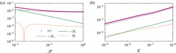
Figure 13 shows the damping rate and its three contributions for two axisymmetric modes: the H mode in figure 6(b), and the HT mode of figure 8. We note that the impact of differential rotation is marginal for both of these modes. Indeed, as shown in the left panel, the thermal dissipation
 $\mathscr{D}_{t}$
dominates at low Prandtl numbers, while the viscous dissipation
 $\mathscr{D}_{v}$
dominates at higher values. The thermal dissipation roughly scales as the expected
 $\mathscr{P}^{-1}$
, and both the viscous and differential rotation dissipations do not scale with
 $\mathscr{P}$
. Interestingly, we see that the sign of the term arising from differential rotation changes sign upon varying
 $\mathscr{P}$
. However, since its magnitude is much smaller than the viscous and thermal dissipation terms, it has a negligible impact on the net damping rate.
For the mode followed on figure 13(b), we see that the viscous dissipation dominates (as
 $\mathscr{P}=1$
). The thermal and viscous dissipation terms follow the same scaling
 $\mathscr{D}_{v},\mathscr{D}_{t}\sim E^{1/2}$
. This is expected from Dintrans et al. (Reference Dintrans, Rieutord and Valdettaro1999): as the width of the shear layers around the attractor scales with
 $E^{1/4}$
, we expect the terms
 $\mathscr{D}_{t}$
and
 $\mathscr{D}_{v}$
to scale with
 $E^{1/2}$
. Expanding the velocity and temperature perturbations in a series of powers of the square root of the Ekman number, it appears that
 $v_{{\it\phi}}=\text{i}v_{r}$
at first order (Rieutord et al.
Reference Rieutord, Georgeot and Valdettaro2001). This phase relation implies that the differential rotation integral
 $\mathscr{D}_{r}$
vanishes at first order. Actually, the way
 $\mathscr{D}_{r}$
scales with
 $E$
or
 $\mathscr{P}$
is different from the other terms and cannot be described without a precise boundary layer analysis.
Growth rate
 ${\it\tau}$
and dissipation terms as a function of the Ekman number, for the unstable wedge-trapped mode displayed in figure 9.
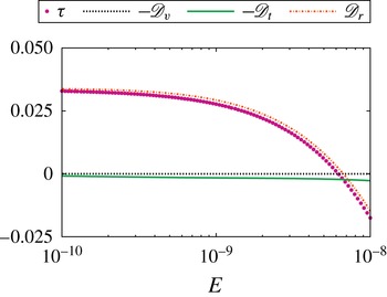
Figure 14 shows the contributions to the damping/growth rate of the wedge-trapped mode shown in figure 9. We find that the contribution of the differential rotation term to the net damping/growth rate is by far the largest, and changes sign in this specific case.
For a regular mode, such as the one presented in figure 12 where the kinetic energy very slightly depends on the Ekman and Prandtl numbers, equation (4.8) predicts that the damping rate should be a linear combination of the viscosity
 ${\it\nu}$
and the thermal dissipation
 ${\it\kappa}$
. The scalings we find are in overall agreement with this expectation and seem to confirm the regular nature of the modes in the range of parameters that we have explored; it is likely that this property extends to actual astrophysical values.
5 Concluding remarks and astrophysical perspectives
In this paper, we have studied the properties of gravito-inertial modes in a differentially rotating spherical shell. Our simplified model unveiled a very rich dynamics that we investigated in two different ways: (i) by studying the linearised oscillation problem in the non-dissipative limit, and (ii) by solving numerically the fully dissipative eigenproblem with a spectral solver. This study emphasises the need to account for stratification, rotation and shear, as they all have a significant impact on the modes’ propagation properties and dissipations.
In the non-dissipative limit, the fluid equations can be recast as a second-order partial differential equation of mixed type. From the paths of characteristics associated with this equation, we found two kinds of gravito-inertial modes: H modes that can propagate in the whole shell, and HT modes that can propagate in a part of the shell bounded by turning surfaces and the shell’s boundaries. Scanning the
 $(N^{2},{\it\omega})$
parameter space (
 $N^{2}$
being the squared surface Brunt–Väisälä frequency, and
 ${\it\omega}$
the wave’s frequency in the inertial frame), we determined the occurrence of both H and HT modes. We found that the frequency domain reachable for HT modes with differential rotation is wider compared to gravito-inertial modes with solid-body rotation, or inertial modes with comparable differential rotation. We have also described the various geometries of HT modes. For both H and HT modes, we computed the paths of characteristics, which often converge towards so-called attractors. We have assessed the presence of attractors and determined the strength of the associated focussing by estimating their Lyapunov exponent. When turning surfaces form an acute angle with one of the boundaries of the domain, we found that the attractors tend towards the singular wedge. Another singularity we have seen is the presence of critical latitudes, where characteristics are tangent to the inner or outer shell boundaries. Non-axisymmetric HT modes also exhibit corotation resonances where the Doppler-shifted frequency vanishes. We determined the corotating radius, which may be inside the propagation region of the shell or be fully inside the elliptic region. We have determined the associated range of parameters in both cases. We have shown that the waves can cross the corotation resonance when the latter is inside the propagation domain. For both axisymmetric and non-axisymmetric modes, we also discussed the baroclinic and shear instabilities expected to appear in our set-up and assessed their probable occurrence.
High-resolution numerical solutions were carried out to explore the waves’ propagation properties in the fully dissipative case. These simulations confirm many predictions of our analytic study of the non-dissipative limit. We computed the kinetic energy distribution in the shell, confirming the expected propagation domain geometries. Our calculations have highlighted a broad variety of gravito-inertial modes: (i) modes with thin shear layers distributed over attractors of characteristics, (ii) wedge-trapped modes potentially amplified by the ABCD instability at low dissipation, (iii) modes that feature a strong shear layer emitted at the critical latitude tangent to the inner core, (iv) modes with corotation resonances inside the propagation domain which are sometimes found to be linearly unstable and (v) quasi-regular modes whose kinetic energy is almost independent of the dissipative parameters in the studied range.
Studying the damping rates of the various categories of modes and their dependence with the Ekman and Prandtl numbers, we often found power laws, some of which could be related to the thickness of the shear layers shaping the mode. In the case of a positive growth rate, we obtain clear evidence of the dominant role of the differential rotation in the rise of the instability.
One of the interesting results of the foregoing study is that unstable modes are not so common regarding the list of instabilities that are possibly present in this set-up. Most probably, the criteria deciding of the existence of such instabilities, which are based on a local analysis, are too loose for the set of modes we have considered. Likely, at higher
 $m$
, with lower Ekman or Prandtl numbers unstable modes are more frequent, but this needs to be confirmed by future work.
In the astrophysics perspective, the results of the present work are interesting in two respects. First, the results show that even with a very simplified set-up, the low-frequency spectrum of a rotating, stably stratified spherical layer is quite complex, collecting many different types of modes, shaped both by turning surfaces and various attractors of characteristics. It leaves a daunting perspective when we have to consider more realistic configurations including two-dimensional differential rotation
 ${\it\Omega}(r,{\it\theta})$
, compressibility effects and magnetic fields.
The good news however, is that some large-scale modes may be unstable and oscillatory. As we showed, the associated instability is directly related to the differential rotation either for axisymmetric modes or non-axisymmetric ones. The determination of the true nature of the instability needs a specific study. Indeed, in such a set-up, large-scale modes could destabilize and destroy the background flow. This is however unlikely: the shear of baroclinic flow is expected to feed small-scale turbulence (e.g. Zahn Reference Zahn1992, or our § 2.4.2), resulting in a turbulent viscosity that may prevent large-scale mode growth, or ease their saturation. If such unstable oscillations do not disappear into a turbulent flow, and saturate in some way (by mode coupling for instance, e.g. Gastine & Dintrans Reference Gastine and Dintrans2008), the stellar oscillation spectrum will be enriched with modes that are specifically dependent on the differential rotation and thus open a window on the internal dynamics of the stars.
In another perspective, the properties of the oscillation spectrum of a star also impact the response of the star or a planet to a tidal excitation. The modes shaped by attractors of characteristics are known to be effective at dissipating energy (Rieutord & Valdettaro Reference Rieutord and Valdettaro2010), but the existence of dynamically unstable modes may change somehow the response of the star. However, as for the free oscillations discussed above, this new kind of modes demands fully nonlinear calculations to determine the actual consequences of the instability on the global dynamics of the star. We leave this study to future work.
Acknowledgements
The authors thank the anonymous referees for their useful comments, B. Dintrans, V. Prat and F. Lignières for useful discussions. The numerical calculations have been carried out on the CalMip machine of the ‘Centre Interuniversitaire de Calcul de Toulouse’ (CICT), which is gratefully acknowledged.
Appendix A. Derivation of the generalized Poincaré operator
In this appendix, we give the full derivation of the generalized Poincaré operator defined in § 3.1.
The equation of motion, with no thermal diffusion and no viscosity, reads
 $$\begin{eqnarray}\displaystyle \partial _{t}\boldsymbol{u}+{\it\Omega}\partial _{{\it\phi}}\boldsymbol{u}+2\boldsymbol{{\it\Omega}}\times \boldsymbol{u}+s(\boldsymbol{u}\boldsymbol{\cdot }\boldsymbol{{\rm\nabla}}{\it\Omega})\boldsymbol{e}_{{\it\phi}}=-\frac{1}{{\it\rho}_{0}}\boldsymbol{{\rm\nabla}}P+N^{2}T\boldsymbol{r}. & & \displaystyle\end{eqnarray}$$
We replace time derivatives using
 $\partial _{t}=\text{i}{\it\omega}$
and define
 $\widetilde{{\it\omega}}={\it\omega}+m{\it\Omega}$
. The heat equation then gives
 $$\begin{eqnarray}\displaystyle T=-\frac{ru_{r}}{\text{i}\widetilde{{\it\omega}}}. & & \displaystyle\end{eqnarray}$$
Projecting (A 1) on the vector basis
 $(\boldsymbol{e}_{s},\boldsymbol{e}_{{\it\phi}},\boldsymbol{e}_{z})$
, using
 $\boldsymbol{e}_{r}=\sin {\it\theta}\boldsymbol{e}_{s}+\cos {\it\theta}\boldsymbol{e}_{z}$
, and
 $r\cos {\it\theta}=z,r\sin {\it\theta}=s$
, we get
 $$\begin{eqnarray}\displaystyle & \displaystyle \text{i}\widetilde{{\it\omega}}u_{s}-2{\it\Omega}u_{{\it\phi}}=-\partial _{s}p-\frac{N^{2}}{\text{i}\widetilde{{\it\omega}}}(s^{2}u_{s}+szu_{z}), & \displaystyle\end{eqnarray}$$
 $$\begin{eqnarray}\displaystyle & \displaystyle \text{i}\widetilde{{\it\omega}}u_{{\it\phi}}+2{\it\Omega}u_{s}+s\partial _{s}{\it\Omega}u_{s}+s\partial _{z}{\it\Omega}u_{z}=-\frac{\text{i}mp}{s}, & \displaystyle\end{eqnarray}$$
 $$\begin{eqnarray}\displaystyle & \displaystyle \text{i}\widetilde{{\it\omega}}u_{z}=-\partial _{z}p-\frac{N^{2}}{\text{i}\widetilde{{\it\omega}}}(szu_{s}+z^{2}u_{z}). & \displaystyle\end{eqnarray}$$
Combining (A 3) and (A 5), we get
 $$\begin{eqnarray}\displaystyle & \displaystyle u_{z}=\frac{\text{i}\widetilde{{\it\omega}}\partial _{z}p+N^{2}szu_{s}}{\widetilde{{\it\omega}}^{2}-N^{2}z^{2}}, & \displaystyle\end{eqnarray}$$
 $$\begin{eqnarray}\displaystyle & \displaystyle u_{{\it\phi}}=\frac{1}{2{\it\Omega}}\left[\frac{\text{i}\widetilde{{\it\omega}}(\widetilde{{\it\omega}}^{2}-N^{2}r^{2})}{\widetilde{{\it\omega}}^{2}-N^{2}z^{2}}u_{s}+\frac{N^{2}sz}{\widetilde{{\it\omega}}^{2}-N^{2}z^{2}}\partial _{z}p+\partial _{s}p\right]. & \displaystyle\end{eqnarray}$$
We replace
 $u_{z}$
and
 $u_{{\it\phi}}$
in (A 4) to obtain
 $$\begin{eqnarray}\displaystyle u_{s} & = & \displaystyle -\frac{\text{i}\widetilde{{\it\omega}}(\widetilde{{\it\omega}}^{2}-N^{2}z^{2})}{A_{s}(\widetilde{{\it\omega}}^{2}-N^{2}z^{2})-\widetilde{{\it\omega}}^{2}(\widetilde{{\it\omega}}^{2}-N^{2}r^{2})+A_{z}N^{2}sz}\nonumber\\ \displaystyle & & \displaystyle \times \,\left[\frac{N^{2}sz+A_{z}}{\widetilde{{\it\omega}}^{2}-N^{2}z^{2}}\partial _{z}p+\partial _{s}p-\frac{2\text{i}m{\it\Omega}}{\text{i}\widetilde{{\it\omega}}s}p\right],\end{eqnarray}$$
with
 $$\begin{eqnarray}\displaystyle A_{s}=\frac{2{\it\Omega}}{s}\frac{\partial }{\partial s}(s^{2}{\it\Omega})\quad \text{and}\quad A_{z}=\frac{2{\it\Omega}}{s}\frac{\partial }{\partial z}(s^{2}{\it\Omega}). & & \displaystyle\end{eqnarray}$$
Using these expressions in the mass conservation equation, keeping only the second-order terms, we finally get (3.1):
 $$\begin{eqnarray}\displaystyle (N^{2}z^{2}-\widetilde{{\it\omega}}^{2})\frac{\partial ^{2}p}{\partial s^{2}}-(2N^{2}sz+A_{z})\frac{\partial ^{2}p}{\partial s\partial z}+(A_{s}+N^{2}s^{2}-\widetilde{{\it\omega}}^{2})\frac{\partial ^{2}p}{\partial z^{2}}=0. & & \displaystyle\end{eqnarray}$$