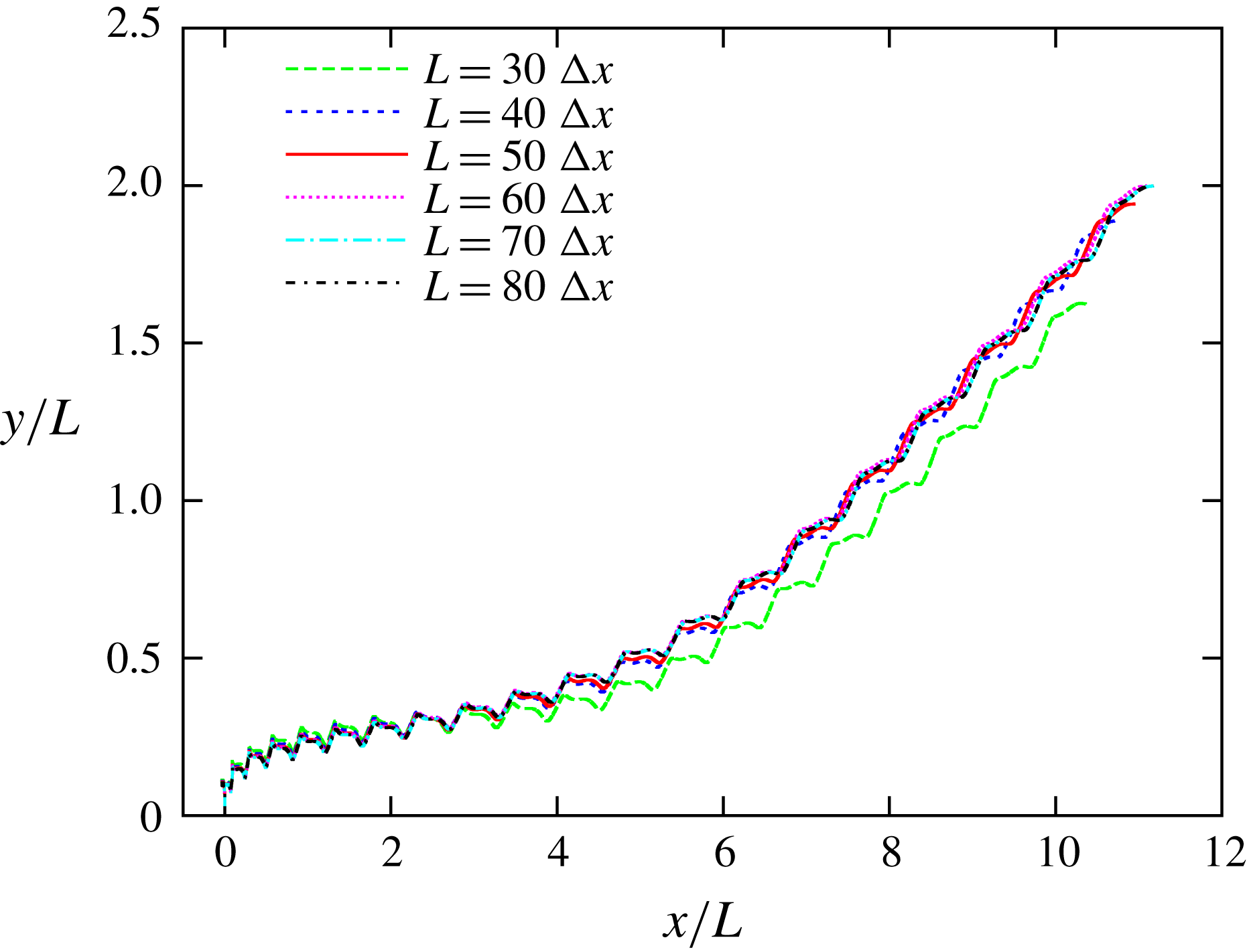
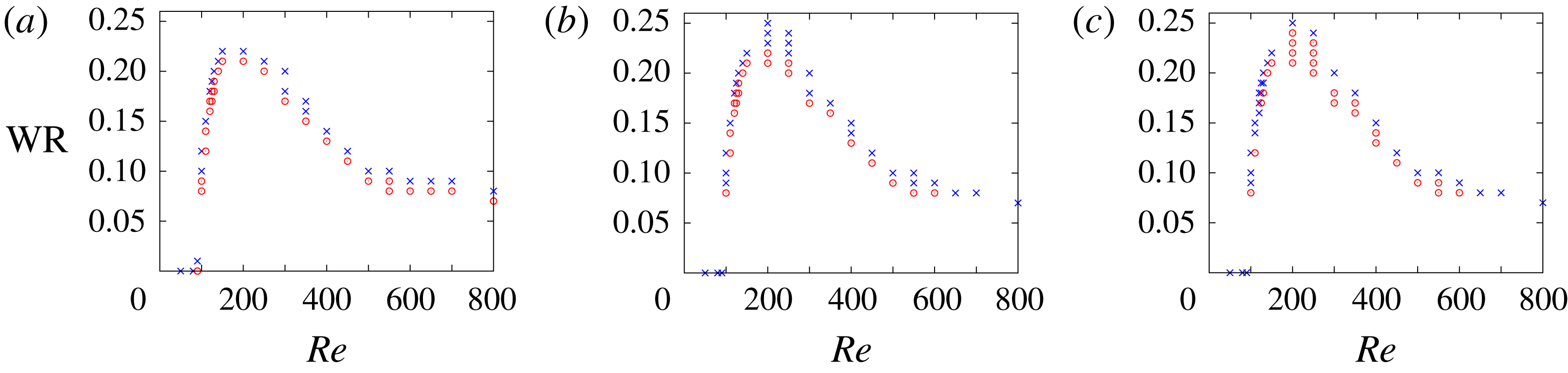
1 Introduction
Butterflies have unique and interesting features compared with other insects. The most conspicuous example is their erratic trajectory and large variation in speed (Shyy et al. Reference Shyy, Aono, Kang and Liu2013; Fei & Yang Reference Fei and Yang2015). This behaviour suggests that butterflies have outstanding agility and manoeuvrability, which are attractive features in practical applications such as micro air vehicles (MAVs) (Ellington Reference Ellington1999). From a biological viewpoint, it has been suggested that butterflies developed erratic flight as an evolutionary response to aerial predation, i.e. for evading other insects and birds attempting to capture them (Dudley Reference Dudley2002). From other viewpoints, in order to incorporate these outstanding features into MAVs, we have to know the physical reasons for the erratic behaviour of butterflies.
It has been suggested that the erratic behaviour of butterflies is mainly caused by their low flapping frequency and their broad wings (Shyy et al. Reference Shyy, Aono, Kang and Liu2013; Fei & Yang Reference Fei and Yang2015). The former makes the body response time scale larger than that for other insects, and the latter enables butterflies to generate large aerodynamic forces abruptly in each stroke. From a viewpoint of wing kinematics, butterflies flap their wings downward to generate lift force and backward to generate thrust force by changing their wing stroke plane (Sunada et al. Reference Sunada, Kawachi, Watanabe and Azuma1993b ), whereas other insects seldom change their stroke plane. This suggests that butterflies utilize aerodynamic forces parallel to the wing-tip path, i.e. the drag-based force (Ellington Reference Ellington1999; Ristroph et al. Reference Ristroph, Bergou, Guckenheimer, Wang and Cohen2011). The peak value of the drag-based force is much larger than that of the aerodynamic forces perpendicular to the wing-tip path, i.e. the lift-based force (Jones et al. Reference Jones, Laurenza, Hedrick, Griffith and Miller2015), and therefore such wing kinematics are likely to be a cause of the erratic behaviour of butterflies. Actually, the simplified wing kinematics of butterflies can generate larger instantaneous aerodynamic forces than revolving wings (Suzuki & Yoshino Reference Suzuki and Yoshino2017).
Unlike the studies of insects in hovering or in steady forward flight, the studies of butterflies have focused on free flight in order to clarify the causes of their erratic behaviour. The importance of studying the free flight of butterflies has been experimentally demonstrated by Srygley & Thomas (Reference Srygley and Thomas2002). They observed butterflies (Vanessa atalanta) in free flight and investigated the air flow around their wings by using high-resolution, smoke-wire flow visualization. They showed that free-flying butterflies use a variety of aerodynamic mechanisms and rapidly switch between them by slightly changing the wing kinematics unlike insects in tethered experiments. They suggested that the rapid shift between aerodynamic mechanisms and consequent large changes in the aerodynamic force may be a cause of the erratic behaviour of butterflies. Since their study emphasized the importance of studying the free flight of butterflies, some researchers have investigated free-flying butterflies experimentally. For example, Takahashi et al. (Reference Takahashi, Tanaka, Matsumoto and Shimoyama2012) measured directly the differential pressure of the flapping wings of free-flying butterflies (Papilio protenor) by using a light pressure sensor developed using microelectromechanical systems. Kang et al. (Reference Kang, Cranford, Sridhar, Kodali, Landrum and Slegers2018) provided detailed data on the kinematics and trajectories of free-flying monarch butterflies (Danaus plexippus).
Although the experimental studies mentioned above have led to a better understanding of the free flight of butterflies, the effect of the inertial force and torque created by the wings of free-flying butterflies has not been studied. The inertial force and torque created by butterfly wings are likely to be much larger than those of other insects, since the wings of butterflies are relatively heavier than those of other insects. The wing-mass ratio (
 $\text{W}\text{R}$
), which is defined as the ratio of the wing mass to the total mass, of butterflies is of
 $O(10^{-1})$
(Dudley Reference Dudley1990), whereas that of other insects such as flies and bees is of
 $O(10^{-2})$
(Shyy et al.
Reference Shyy, Lian, Tang, Viieru and Liu2008). Therefore, it is expected that the inertial force and torque created by butterfly wings will have a significant effect on agility and manoeuvrability during free flight. Actually, the inertial force was found to be significant relative to the aerodynamic force in hawkmoths (Daniel & Combes Reference Daniel and Combes2002; Combes & Daniel Reference Combes and Daniel2003), which are similar in size to butterflies. In addition, in our previous study using a two-dimensional model with symmetric flapping wings and a body (Suzuki, Aoki & Yoshino Reference Suzuki, Aoki and Yoshino2017), we found that for a large
 $\text{W}\text{R}$
the body has a large vertical oscillation during each stroke due to the inertial force created by the wings, and the aerodynamic force decreases due to the body motion. Therefore, it is important to investigate the interaction between the inertial and aerodynamic forces and torques and the body motion. However, the effect of the inertial force and torque, i.e. the effect of the wing mass, on the free flight of butterflies has not been investigated comprehensively.
Since it has been difficult to experimentally investigate the interaction between the inertial and aerodynamic forces and torques and the body motion, a numerical approach is attractive for investigating such interactions in the free flight of butterflies. Although there have been several numerical studies of the free flight of butterflies, most of these kinds of studies have neglected the effect of the wing mass. Suzuki, Minami & Inamuro (Reference Suzuki, Minami and Inamuro2015) constructed a simple butterfly-like model and investigated numerically its lift and thrust generation, free flight and attitude control. This model is composed of two infinitely thin square wings and a rod-shaped body, and it flaps downward to generate lift force and backward to generate thrust force like an actual butterfly. In their study, the flow field around the model and the aerodynamic force and torque acting on the wings were computed by the immersed boundary–lattice Boltzmann method (IB-LBM) (Suzuki & Inamuro Reference Suzuki and Inamuro2011). It was found that the butterfly-like model can generate enough lift force to support an actual butterfly’s weight in free flight, even though it is a highly idealized and simplified model of an actual butterfly. However, the mass of the wings was neglected and consequently the inertial force and torque created by the wings were not investigated. In the subsequent work by Nakatani, Suzuki & Inamuro (Reference Nakatani, Suzuki and Inamuro2016) investigating some control strategies, the mass of the wings was neglected as well. More recently, Fei & Yang (Reference Fei and Yang2015, Reference Fei and Yang2016) created a numerical model of a butterfly based on the experimental record of the flight motion of the leaf butterfly (Kallima inachus) and investigated the effect of body translation and rotation on the aerodynamic force and flow field. In this numerical model, however, the mass of the wings was also neglected.
Only a few numerical studies have incorporated wing mass into the model. Sunada et al. (Reference Sunada, Kawachi, Watanabe and Azuma1993b ) observed a butterfly (Pieris melete) in take-off flight and analysed its motion from aerodynamic and kinetic viewpoints. In their analysis, the aerodynamic force and torque acting on the butterfly’s wings were calculated by the vortex method (Sunada et al. Reference Sunada, Kawachi, Watanabe and Azuma1993a ) and by their proposed simple method. In addition, they measured the mass of the butterfly’s wings and calculated the inertial force and torque created by the wings. They found that the inertial force and torque were much smaller than the aerodynamic force and torque, respectively. However, this seems to contradict the recent study by Lin et al. (Reference Lin, Zheng, Hedrick and Mittal2012). They conducted detailed observations and measurements of the free flight of a butterfly (Vanessa cardui), and it was concluded that interactions between the inertial and aerodynamic torques may substantially influence the butterfly’s flight manoeuvres. Yokoyama et al. (Reference Yokoyama, Senda, Iima and Hirai2013) computed forward flights of a butterfly (Parantica sita) modelled as a four-link rigid-body system consisting of a thorax, an abdomen and left and right wings. In their simulation, the flow field around the model and the aerodynamic force and torque acting on the wings were computed by the spectral method with the immersed boundary method (Mittal & Iaccarino Reference Mittal and Iaccarino2005), and the motion of the four-link rigid-body system was calculated by solving the Euler–Lagrangian equation of motion with not only the aerodynamic force and torque but also the inertial force and torque created by the wings with non-zero mass. Therefore, their study considered the interaction between the inertial and aerodynamic forces and torques and the body motion precisely. Unfortunately, their study did not clarify the magnitude of the inertial force and torque compared with the aerodynamic force and torque.
As seen from the above discussion, the effect of the inertial force and torque created by the wings of a free-flying butterfly has not been clarified. Therefore, the following question still remains open: ‘How does the wing mass affect the free flight of butterflies?’ This question is important in the development of flapping MAVs, since the wing-mass ratio of such vehicles can be of
 $O(1)$
(Shyy et al.
Reference Shyy, Aono, Kang and Liu2013). In the present study, we attempt to answer the above question by a computational approach using the butterfly-like model proposed by Suzuki et al. (Reference Suzuki, Minami and Inamuro2015). Since the original model did not have wing mass, we add wing mass to the model and investigate the effect of wing mass on the free flight of the model. While there might be some flight modes in the free flight of butterflies, e.g. take-off, climbing flight, forward flight and gliding flight, we focus on a take-off from the resting state and the transitional motion to a forward flight.
The paper is organized as follows. In § 2, we present the butterfly-like model with wing mass. In § 3, we explain the governing equations and parameters of the system. The computational parameters are presented in § 4, and results and discussion in § 5. We discuss the limitations of the model in § 6. We finally conclude in § 7.
2 Butterfly-like model
We add wing mass to the butterfly-like model originally proposed by Suzuki et al. (Reference Suzuki, Minami and Inamuro2015) to investigate the effect of wing mass on the free flight of butterflies. The reason why we use such an idealized model is as follows. An actual butterfly has many factors that affect its motion, e.g. the kinematics, planform, structure, mass and flexibility of the wings and also the motion, structure and mass of the body, and they interact in a complex way. Using a realistic model of a butterfly, therefore, we cannot distinguish which factors are significant or trivial. On the other hand, an idealized model makes it relatively easy to investigate the effect of each factor individually. Actually, the individual effects of the wing kinematics and of the wing planform on the aerodynamic performance were investigated effectively by using this model (Suzuki et al. Reference Suzuki, Minami and Inamuro2015; Suzuki & Yoshino Reference Suzuki and Yoshino2017, Reference Suzuki and Yoshino2018). Comprehensive parametric studies using this model will give valuable data for the design of insect-inspired MAVs. Therefore, this model is appropriate for the investigation of the effect of wing mass on aerodynamic performance. However, there might be some limitations of the model due to the many simplifications. The limitations of the model are discussed in § 6.
In the following, we first introduce the components of the model, and then we describe the wing kinematics of the model.
2.1 Components
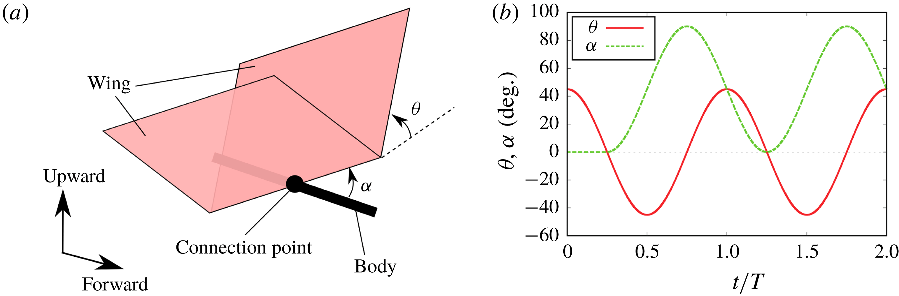
The model used in this paper is shown in figure 1(a). It is a simple wing–body model with infinitely thin square wings of side length
 $L$
and a rod-shaped body of length
 $L_{b}=L$
. The wing root is connected to the mid-point of the body. The flexibility of the wings is neglected. However, the mass of the wings is considered in the present study. The total mass of the two wings is denoted by
 $m_{w}$
(the mass distribution of the wings is described below). The body has a uniform (line) density
 $\unicode[STIX]{x1D70C}_{b}$
. Therefore, the centre of mass of the body is at its mid-point, and the mass and moment of inertia of the body are
 $m_{b}=\unicode[STIX]{x1D70C}_{b}L_{b}$
and
 $I_{b}=m_{b}L_{b}^{2}/12$
, respectively. The total mass of the model is
 $M=m_{w}+m_{b}$
. We define the wing-mass ratio (
 $\text{W}\text{R}$
) as follows:
 $$\begin{eqnarray}\text{W}\text{R}=\frac{m_{w}}{m_{w}+m_{b}}=\frac{m_{w}}{M}.\end{eqnarray}$$
In the present study, we simulate the free flight of the butterfly-like model by changing the values of
 $\text{W}\text{R}$
.
(a) Perspective illustration of the butterfly-like model. The wings are infinitely thin and square of side length
 $L$
. The length of the body is
 $L_{b}=L$
. (b) Time variations of the angle of attack
 $\unicode[STIX]{x1D6FC}$
and the flapping angle
 $\unicode[STIX]{x1D703}$
during the first two periods (
 $0\leqslant t/T\leqslant 2$
) when
 $\unicode[STIX]{x1D703}_{m}=45^{\circ }$
,
 $\unicode[STIX]{x1D6FC}_{m}=90^{\circ }$
and
 $\unicode[STIX]{x1D6FE}=\unicode[STIX]{x03C0}/2$
.

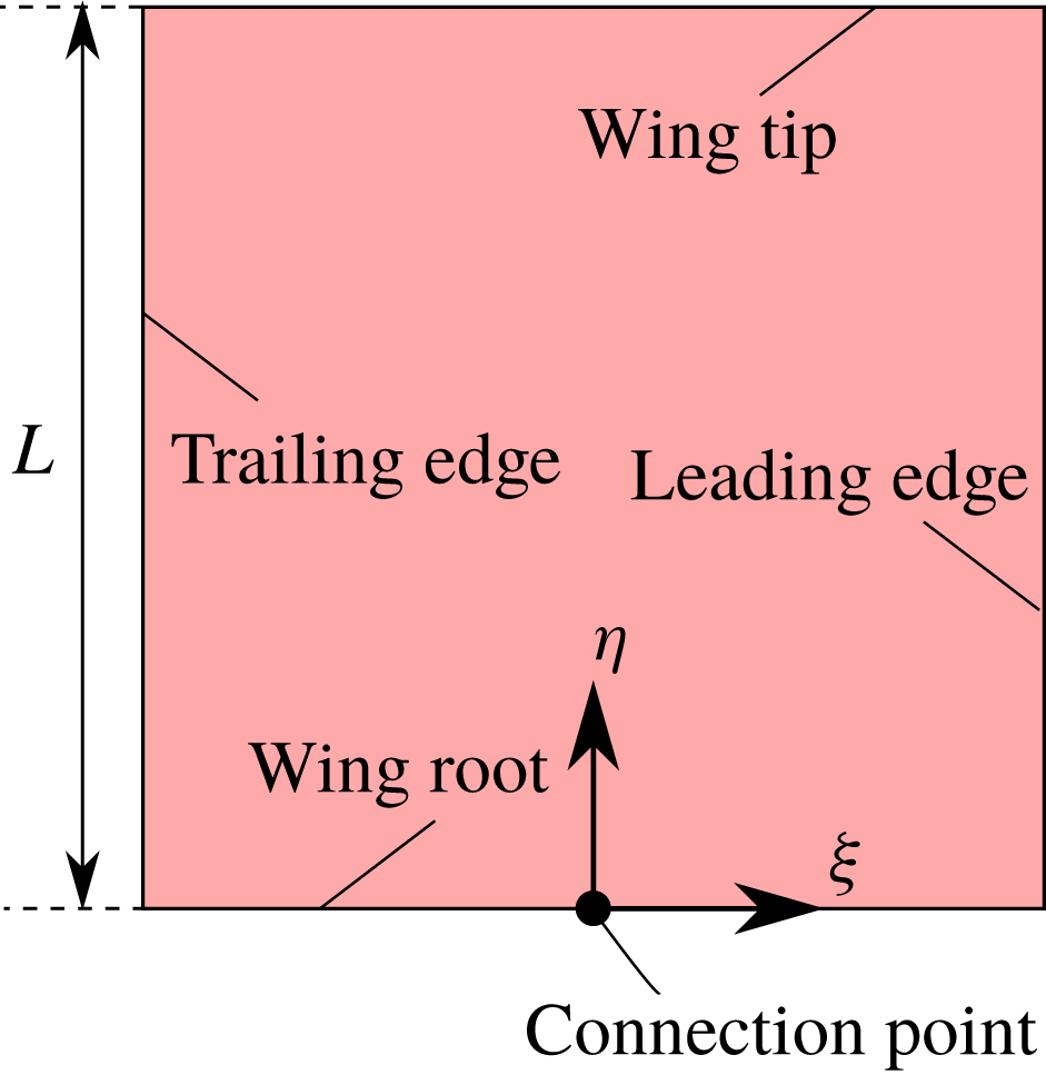
In order to describe the wing-mass distribution, we define the coordinate system as shown in figure 2 for the right-hand wing. The axes are
 $\unicode[STIX]{x1D709}$
,
 $\unicode[STIX]{x1D702}$
and
 $\unicode[STIX]{x1D701}$
and the origin is located at the middle point of the wing root. Letting the
 $\unicode[STIX]{x1D709}$
- and
 $\unicode[STIX]{x1D702}$
-axes be parallel to the chord direction and the span direction, respectively, the wing-mass distribution is a function of
 $\unicode[STIX]{x1D709}$
and
 $\unicode[STIX]{x1D702}$
denoted by
 $\unicode[STIX]{x1D70C}_{w}(\unicode[STIX]{x1D709},\unicode[STIX]{x1D702})$
. The relationship between the wing mass
 $m_{w}$
and the wing-mass distribution
 $\unicode[STIX]{x1D70C}_{w}(\unicode[STIX]{x1D709},\unicode[STIX]{x1D702})$
can be written as
 $$\begin{eqnarray}m_{w}=2\int _{wing}\unicode[STIX]{x1D70C}_{w}(\unicode[STIX]{x1D709},\unicode[STIX]{x1D702})\,\text{d}\unicode[STIX]{x1D709}\,\text{d}\unicode[STIX]{x1D702},\end{eqnarray}$$
where
 $\int _{wing}\,\text{d}\unicode[STIX]{x1D709}\,\text{d}\unicode[STIX]{x1D702}$
means the integral over the right-hand wing. Since the Lagrangian of the system is calculated by integrating the kinetic and potential energies over the wings (see § 3.2), the wing-mass distribution affects the motion of the model through the integral forms listed below:
 $$\begin{eqnarray}\displaystyle & \displaystyle R_{\unicode[STIX]{x1D709}}=\frac{2}{m_{w}}\int _{wing}\unicode[STIX]{x1D709}\unicode[STIX]{x1D70C}_{w}(\unicode[STIX]{x1D709},\unicode[STIX]{x1D702})\,\text{d}\unicode[STIX]{x1D709}\,\text{d}\unicode[STIX]{x1D702}, & \displaystyle\end{eqnarray}$$
 $$\begin{eqnarray}\displaystyle & \displaystyle R_{\unicode[STIX]{x1D702}}=\frac{2}{m_{w}}\int _{wing}\unicode[STIX]{x1D702}\unicode[STIX]{x1D70C}_{w}(\unicode[STIX]{x1D709},\unicode[STIX]{x1D702})\,\text{d}\unicode[STIX]{x1D709}\,\text{d}\unicode[STIX]{x1D702}, & \displaystyle\end{eqnarray}$$
 $$\begin{eqnarray}\displaystyle & \displaystyle \unicode[STIX]{x1D61A}_{\unicode[STIX]{x1D709}\unicode[STIX]{x1D709}}=\frac{2}{m_{w}}\int _{wing}\unicode[STIX]{x1D709}^{2}\unicode[STIX]{x1D70C}_{w}(\unicode[STIX]{x1D709},\unicode[STIX]{x1D702})\,\text{d}\unicode[STIX]{x1D709}\,\text{d}\unicode[STIX]{x1D702}, & \displaystyle\end{eqnarray}$$
 $$\begin{eqnarray}\displaystyle & \displaystyle \unicode[STIX]{x1D61A}_{\unicode[STIX]{x1D709}\unicode[STIX]{x1D702}}=\frac{2}{m_{w}}\int _{wing}\unicode[STIX]{x1D709}\unicode[STIX]{x1D702}\unicode[STIX]{x1D70C}_{w}(\unicode[STIX]{x1D709},\unicode[STIX]{x1D702})\,\text{d}\unicode[STIX]{x1D709}\,\text{d}\unicode[STIX]{x1D702}, & \displaystyle\end{eqnarray}$$
 $$\begin{eqnarray}\displaystyle & \displaystyle \unicode[STIX]{x1D61A}_{\unicode[STIX]{x1D702}\unicode[STIX]{x1D702}}=\frac{2}{m_{w}}\int _{wing}\unicode[STIX]{x1D702}^{2}\unicode[STIX]{x1D70C}_{w}(\unicode[STIX]{x1D709},\unicode[STIX]{x1D702})\,\text{d}\unicode[STIX]{x1D709}\,\text{d}\unicode[STIX]{x1D702}. & \displaystyle\end{eqnarray}$$
The vector
 $(R_{\unicode[STIX]{x1D709}},R_{\unicode[STIX]{x1D702}})$
corresponds to the position of the centre of mass of the wing, and the matrix
 $\unicode[STIX]{x1D61A}_{ij}$
(
 $i,j=\unicode[STIX]{x1D709},\unicode[STIX]{x1D702}$
) corresponds to the inertia tensor of the wing divided by the wing mass. In the present study, we consider various sets of the above parameters by changing the wing-mass distribution
 $\unicode[STIX]{x1D70C}_{w}(\unicode[STIX]{x1D709},\unicode[STIX]{x1D702})$
.
The coordinate system of the right-hand wing. The
 $\unicode[STIX]{x1D709}$
-axis and
 $\unicode[STIX]{x1D702}$
-axis are parallel to the chord direction and the span direction, respectively.

2.2 Wing kinematics
The butterfly-like model flaps its wings downward and backward to generate lift and thrust forces, respectively. The motions of the two wings are prescribed relative to the body and are symmetric with respect to the longitudinal plane. The wing kinematics are a combination of a flapping motion and an attacking motion, described by the flapping angle
 $\unicode[STIX]{x1D703}$
and the angle of attack (AOA)
 $\unicode[STIX]{x1D6FC}$
, respectively, as shown in figure 1. The rotational axis for the AOA is perpendicular to the wing root, and that for the flapping angle is parallel to the wing root. The flapping angle
 $\unicode[STIX]{x1D703}(t)$
and the AOA
 $\unicode[STIX]{x1D6FC}(t)$
at time
 $t$
are given as follows:
 $$\begin{eqnarray}\displaystyle & \displaystyle \unicode[STIX]{x1D703}(t)=\unicode[STIX]{x1D703}_{m}\cos \left(\frac{2\unicode[STIX]{x03C0}}{T}t\right), & \displaystyle\end{eqnarray}$$
 $$\begin{eqnarray}\displaystyle & \displaystyle \unicode[STIX]{x1D6FC}(t)=\left\{\begin{array}{@{}ll@{}}0,\quad & \displaystyle \left(0\leqslant t<\frac{T}{4}\right),\\ \displaystyle \frac{\unicode[STIX]{x1D6FC}_{m}}{2}\left[1+\cos \left(\frac{2\unicode[STIX]{x03C0}}{T}t+\unicode[STIX]{x1D6FE}\right)\right],\quad & \displaystyle \left(t\geqslant \frac{T}{4}\right),\end{array}\right. & \displaystyle\end{eqnarray}$$
where
 $\unicode[STIX]{x1D703}_{m}$
is the flapping amplitude corresponding to half the stroke amplitude,
 $\unicode[STIX]{x1D6FC}_{m}$
is the maximum AOA,
 $T$
is the period of flapping motion and
 $\unicode[STIX]{x1D6FE}$
is the phase shift. In our previous study (Suzuki & Yoshino Reference Suzuki and Yoshino2017), we calculated aerodynamic performance for various sets of the kinematic parameters
 $(\unicode[STIX]{x1D703}_{m},\unicode[STIX]{x1D6FC}_{m},\unicode[STIX]{x1D6FE})$
, and found that the efficiency (the time-averaged power-loading coefficient) is nearly maximized when
 $(\unicode[STIX]{x1D703}_{m},\unicode[STIX]{x1D6FC}_{m},\unicode[STIX]{x1D6FE})=(45^{\circ },90^{\circ },\unicode[STIX]{x03C0}/2)$
. Although this set of kinematic parameters is not exactly optimal, we set
 $\unicode[STIX]{x1D703}_{m}=45^{\circ }$
,
 $\unicode[STIX]{x1D6FC}_{m}=90^{\circ }$
and
 $\unicode[STIX]{x1D6FE}=\unicode[STIX]{x03C0}/2$
in this study. The difference between the wing kinematics of the present model and those of actual butterflies is discussed in § 6.2. Figure 1(b) shows the time variations of
 $\unicode[STIX]{x1D6FC}(t)$
and
 $\unicode[STIX]{x1D703}(t)$
for the above set of the parameters. It should be noted that the AOA
 $\unicode[STIX]{x1D6FC}(t)$
given above is different from that used by Suzuki et al. (Reference Suzuki, Minami and Inamuro2015) only in the first quarter period of the first wingbeat. If the time derivative of
 $\unicode[STIX]{x1D6FC}(t)$
is not zero at the initial time
 $t=0$
, the wings have momentum initially due to the wing mass. Therefore, this modification is to avoid an impulsive start. More details about the wing kinematics of the model can be found in Suzuki et al. (Reference Suzuki, Minami and Inamuro2015).
3 Governing equations
3.1 Fluid motion
The fluid motion around the butterfly-like model is governed by the continuity equation and the Navier–Stokes equation for an incompressible fluid
 $$\begin{eqnarray}\displaystyle & \displaystyle \unicode[STIX]{x1D735}\boldsymbol{\cdot }\boldsymbol{u}=0, & \displaystyle\end{eqnarray}$$
 $$\begin{eqnarray}\displaystyle & \displaystyle \frac{\unicode[STIX]{x2202}\boldsymbol{u}}{\unicode[STIX]{x2202}t}+(\boldsymbol{u}\boldsymbol{\cdot }\unicode[STIX]{x1D735})\boldsymbol{u}=-\frac{1}{\unicode[STIX]{x1D70C}_{f}}\unicode[STIX]{x1D735}p+\unicode[STIX]{x1D708}\unicode[STIX]{x1D6FB}^{2}\boldsymbol{u}, & \displaystyle\end{eqnarray}$$
where
 $\boldsymbol{u}$
is the fluid velocity,
 $p$
is the pressure,
 $\unicode[STIX]{x1D70C}_{f}$
is the fluid density and
 $\unicode[STIX]{x1D708}$
is the kinematic viscosity of the fluid. We consider the fluid to be air at room temperature (
 $20\,^{\circ }\text{C}$
), and we set
 $\unicode[STIX]{x1D70C}_{f}=1.205~\text{kg}~\text{m}^{-3}$
and
 $\unicode[STIX]{x1D708}=1.512\times 10^{-5}~\text{m}^{2}~\text{s}^{-1}$
. It should be noted that the gravitational term does not appear in (3.2). This is because the pressure
 $p$
includes the gravitational potential. The no-slip condition must be satisfied on the surface of the model, i.e. the fluid velocity must be equal to the velocity of the wings and the body. It is noted that the body has a negligible effect on the flow field and the aerodynamic forces for the present model, although the no-slip condition is enforced on the body. This is because the body of the model is simplified to be infinitely thin. However, the body with a finite thickness might have a significant effect. We discuss this issue in § 6.1.
In this study, we use the mean wing-tip speed defined by
 $U_{tip}=4\unicode[STIX]{x1D703}_{m}L/T$
as the characteristic flow speed, and the wing length
 $L$
as the characteristic length. The governing non-dimensional parameter of the above equations is the Reynolds number
 $Re$
given by
 $$\begin{eqnarray}Re=\frac{U_{tip}L}{\unicode[STIX]{x1D708}}.\end{eqnarray}$$
Note that the definition of the Reynolds number is the same as that used by Suzuki et al. (Reference Suzuki, Minami and Inamuro2015).
3.2 Wing–body motion
By adding the wing mass to the model, the equations of the wing–body motion become much more complicated than those when the wing mass is neglected. The system of the present model is a three-body problem composed of two rigid flat plates (wings) and one rigid rod (body). In order to make the wings and the body connected and to enforce the flapping angle
 $\unicode[STIX]{x1D703}(t)$
and the AOA
 $\unicode[STIX]{x1D6FC}(t)$
of the wings relative to the body, we have to consider the appropriate force of constraint and torque of constraint between the wings and the body. If the Lagrangian formulation is used, however, there is no need to formulate them explicitly.
We define the coordinate system of the flight space with axes
 $x$
,
 $y$
and
 $z$
, where the positive directions of the
 $x$
-axis and
 $y$
-axis are the forward and upward directions, respectively. The gravitational acceleration is given by
 $\boldsymbol{G}=(0,-G,0)^{\text{T}}$
(where the superscript T represents the transpose of a vector or a matrix), and we set
 $G=9.807~\text{m}~\text{s}^{-2}$
. Here, we assume that the body moves only in the
 $x$
- and
 $y$
-directions and rotates only in the
 $x$
–
 $y$
plane (pitching motion) for simplicity. Let the position of the centre of the body be
 $\boldsymbol{X}_{b}=(x_{b},y_{b},0)^{\text{T}}$
and the pitching angle be
 $\unicode[STIX]{x1D703}_{p}$
. The motion of the wing–body system is described by the three independent variables
 $x_{b}$
,
 $y_{b}$
and
 $\unicode[STIX]{x1D703}_{p}$
. The Lagrangian for the wing–body system is given by
 $$\begin{eqnarray}\displaystyle {\mathcal{L}} & = & \displaystyle {\textstyle \frac{1}{2}}m_{b}({\dot{x}}_{b}^{2}+{\dot{y}}_{b}^{2})+{\textstyle \frac{1}{2}}I_{b}\dot{\unicode[STIX]{x1D703}}_{p}^{2}-m_{b}Gy_{b}\nonumber\\ \displaystyle & & \displaystyle +\,{\textstyle \frac{1}{2}}m_{w}({\dot{x}}_{b}^{2}+{\dot{y}}_{b}^{2})\nonumber\\ \displaystyle & & \displaystyle +\,m_{w}\unicode[STIX]{x1D61A}_{\unicode[STIX]{x1D709}\unicode[STIX]{x1D702}}(\dot{\unicode[STIX]{x1D703}}_{p}+\dot{\unicode[STIX]{x1D6FC}})\dot{\unicode[STIX]{x1D703}}\cos \unicode[STIX]{x1D703}+{\textstyle \frac{1}{2}}m_{w}\unicode[STIX]{x1D61A}_{\unicode[STIX]{x1D709}\unicode[STIX]{x1D709}}(\dot{\unicode[STIX]{x1D703}}_{p}+\dot{\unicode[STIX]{x1D6FC}})^{2}+{\textstyle \frac{1}{2}}m_{w}\unicode[STIX]{x1D61A}_{\unicode[STIX]{x1D702}\unicode[STIX]{x1D702}}\{(\dot{\unicode[STIX]{x1D703}}_{p}+\dot{\unicode[STIX]{x1D6FC}})^{2}\sin ^{2}\unicode[STIX]{x1D703}+\dot{\unicode[STIX]{x1D703}}^{2}\}\nonumber\\ \displaystyle & & \displaystyle +\,m_{w}R_{\unicode[STIX]{x1D709}}(\dot{\unicode[STIX]{x1D703}}_{p}+\dot{\unicode[STIX]{x1D6FC}})\{-{\dot{x}}_{b}\sin (\unicode[STIX]{x1D703}_{p}+\unicode[STIX]{x1D6FC})+{\dot{y}}_{b}\cos (\unicode[STIX]{x1D703}_{p}+\unicode[STIX]{x1D6FC})\}\nonumber\\ \displaystyle & & \displaystyle -\,m_{w}R_{\unicode[STIX]{x1D702}}(\dot{\unicode[STIX]{x1D703}}_{p}+\dot{\unicode[STIX]{x1D6FC}})\sin \unicode[STIX]{x1D703}\{{\dot{x}}_{b}\cos (\unicode[STIX]{x1D703}_{p}+\unicode[STIX]{x1D6FC})+{\dot{y}}_{b}\sin (\unicode[STIX]{x1D703}_{p}+\unicode[STIX]{x1D6FC})\}\nonumber\\ \displaystyle & & \displaystyle +\,m_{w}R_{\unicode[STIX]{x1D702}}\dot{\unicode[STIX]{x1D703}}\cos \unicode[STIX]{x1D703}\{-{\dot{x}}_{b}\sin (\unicode[STIX]{x1D703}_{p}+\unicode[STIX]{x1D6FC})+{\dot{y}}_{b}\cos (\unicode[STIX]{x1D703}_{p}+\unicode[STIX]{x1D6FC})\}\nonumber\\ \displaystyle & & \displaystyle -\,m_{w}G\{y_{b}+R_{\unicode[STIX]{x1D709}}\sin (\unicode[STIX]{x1D703}_{p}+\unicode[STIX]{x1D6FC})+R_{\unicode[STIX]{x1D702}}\cos (\unicode[STIX]{x1D703}_{p}+\unicode[STIX]{x1D6FC})\sin \unicode[STIX]{x1D703}\},\end{eqnarray}$$
where the dot notation denotes the time derivative. The Lagrange equations for the wing–body motion can be obtained as follows:
 $$\begin{eqnarray}\displaystyle & \displaystyle \frac{\text{d}}{\text{d}t}\left(\frac{\unicode[STIX]{x2202}{\mathcal{L}}}{\unicode[STIX]{x2202}{\dot{x}}_{b}}\right)-\frac{\unicode[STIX]{x2202}{\mathcal{L}}}{\unicode[STIX]{x2202}x_{b}}=F_{aero\,x}, & \displaystyle\end{eqnarray}$$
 $$\begin{eqnarray}\displaystyle & \displaystyle \frac{\text{d}}{\text{d}t}\left(\frac{\unicode[STIX]{x2202}{\mathcal{L}}}{\unicode[STIX]{x2202}{\dot{y}}_{b}}\right)-\frac{\unicode[STIX]{x2202}{\mathcal{L}}}{\unicode[STIX]{x2202}y_{b}}=F_{aero\,y}, & \displaystyle\end{eqnarray}$$
 $$\begin{eqnarray}\displaystyle & \displaystyle \frac{\text{d}}{\text{d}t}\left(\frac{\unicode[STIX]{x2202}{\mathcal{L}}}{\unicode[STIX]{x2202}\dot{\unicode[STIX]{x1D703}}_{p}}\right)-\frac{\unicode[STIX]{x2202}{\mathcal{L}}}{\unicode[STIX]{x2202}\unicode[STIX]{x1D703}_{p}}=T_{aero}, & \displaystyle\end{eqnarray}$$
where
 $F_{aero\,x}$
and
 $F_{aero\,y}$
are the
 $x$
- and
 $y$
-components of the aerodynamic force
 $\boldsymbol{F}_{aero}$
, respectively, and
 $T_{aero}$
is the aerodynamic pitching moment.
By substituting (3.4) in (3.5)–(3.7), these equations can be expressed in matrix form for the vector
 $(\ddot{x}_{b},\ddot{y} _{b},\ddot{\unicode[STIX]{x1D703}}_{p})^{\text{T}}$
using variables shown in appendix A as
 $$\begin{eqnarray}\boldsymbol{{\mathcal{M}}}\left[\begin{array}{@{}c@{}}\ddot{x}_{b}\\ \ddot{y} _{b}\\ \ddot{\unicode[STIX]{x1D703}}_{p}\end{array}\right]=\left[\begin{array}{@{}c@{}}F_{aero\,x}+F_{in\,x}\\ F_{aero\,y}+F_{in\,y}-MG\\ T_{aero}+T_{in}+T_{G}\end{array}\right],\end{eqnarray}$$
where
 $\boldsymbol{{\mathcal{M}}}$
is the mass matrix of the system,
 $F_{in\,x}$
and
 $F_{in\,y}$
are the
 $x$
- and
 $y$
-components of the inertial force
 $\boldsymbol{F}_{in}$
, respectively,
 $T_{in}$
is the inertial pitching moment and
 $T_{G}$
is the pitching moment due to gravity. The detailed forms of
 $\boldsymbol{{\mathcal{M}}}$
,
 $\boldsymbol{F}_{in}$
,
 $T_{in}$
and
 $T_{G}$
are shown in appendix A.
The governing non-dimensional parameters of (3.8) are the wing-mass ratio
 $\text{W}\text{R}$
given by (2.1), the non-dimensional total mass
 $N_{M}$
and the Froude number
 $Fr$
defined as
 $$\begin{eqnarray}\displaystyle & \displaystyle N_{M}=\frac{M}{\unicode[STIX]{x1D70C}_{f}L^{3}}, & \displaystyle\end{eqnarray}$$
 $$\begin{eqnarray}\displaystyle & \displaystyle Fr=\frac{U_{tip}}{\sqrt{LG}}. & \displaystyle\end{eqnarray}$$
The governing non-dimensional parameters of the whole system are the Reynolds number
 $Re$
, the wing-mass ratio
 $\text{W}\text{R}$
, the non-dimensional total mass
 $N_{M}$
and the Froude number
 $Fr$
. However, these four non-dimensional parameters are not independent, since we fix the values of
 $\unicode[STIX]{x1D70C}_{f}$
,
 $\unicode[STIX]{x1D708}$
and
 $G$
as constants that will not be changed. Actually, the relationship between
 $Re$
and
 $Fr$
is given by
 $$\begin{eqnarray}\frac{Fr}{Re}=\frac{\unicode[STIX]{x1D708}}{\sqrt{L^{3}G}}.\end{eqnarray}$$
Given the values of
 $\unicode[STIX]{x1D708}$
in the Earth’s atmosphere and
 $G$
, the ratio of
 $Fr$
to
 $Re$
is determined by setting the wing length
 $L$
. Therefore, the wing length
 $L$
is equivalent to the ratio of the Reynolds number to the Froude number in this situation.
4 Numerical method and computational parameters
The numerical method used in this study is the same as that in Suzuki et al. (Reference Suzuki, Minami and Inamuro2015); we use the IB-LBM approach (Suzuki & Inamuro Reference Suzuki and Inamuro2011) to solve (3.1) and (3.2) and we use the second-order Adams–Bashforth method to solve (3.8). The aerodynamic force
 $\boldsymbol{F}_{aero}$
and pitching moment
 $T_{aero}$
are calculated by the summation of the volume force which is applied to enforce the no-slip condition on the model in the immersed boundary method. In this calculation, the internal mass effect (see Suzuki & Inamuro Reference Suzuki and Inamuro2011) is neglected, since the model has no volume. The wings and the body of the model are represented by an arrangement of boundary Lagrangian points. The position and velocity of the boundary Lagrangian points on the wings and the body are updated by orthogonal transformation of the coordinate systems fixed to the wings and the body relative to that fixed to the flight space. The validation of the numerical method and the convergence studies for temporal and spatial resolutions have been extensively checked in Suzuki et al. (Reference Suzuki, Minami and Inamuro2015) and Suzuki & Yoshino (Reference Suzuki and Yoshino2018). In addition, Engels et al. (Reference Engels, Kolomenskiy, Schneider and Sesterhenn2016) simulated the same problem as Suzuki et al. (Reference Suzuki, Minami and Inamuro2015) to validate their proposed method (a Fourier method with volume penalization), and they reported that their result for the free flight of the butterfly-like model had a good agreement with that obtained by Suzuki et al. (Reference Suzuki, Minami and Inamuro2015).
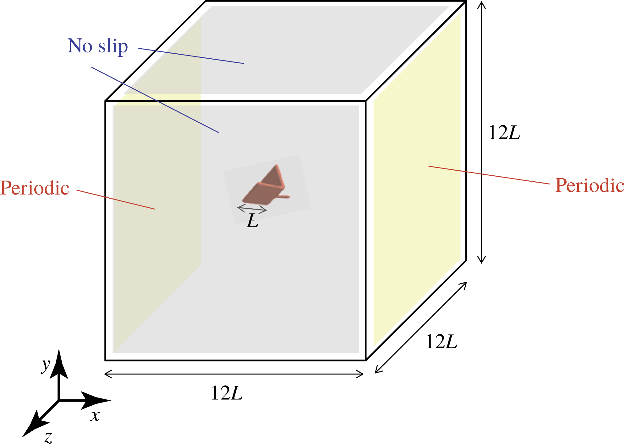
The computational parameters are the same as those described in Suzuki et al. (Reference Suzuki, Minami and Inamuro2015). The computational domain is a cube with a side length equal to
 $W=12L$
as shown in figure 3. The boundary condition on the two sides perpendicular to the
 $x$
-axis is the periodic boundary condition, and on the other sides the no-slip condition is used. The size of the computational domain is so large that the ground effect is negligibly small, since in the previous study by Suzuki et al. (Reference Suzuki, Minami and Inamuro2015) the aerodynamic forces obtained when the domain size was
 $12L\times 6L\times 6L$
were almost the same as those obtained when the domain size was
 $12L\times 12L\times 12L$
. The inner fine grid (Inamuro Reference Inamuro2012) used only around the model is a cube with a side length equal to
 $D=2.4L$
. The centre of the body is initially placed at the centre of the domain, and the fluid in the domain is initially stationary and at a uniform pressure. We simulate free flights of the butterfly-like model for various Reynolds numbers
 $Re<1200$
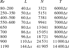
. The spatial and temporal resolutions for each
 $Re$
are shown in table 1. A convergence study is presented in appendix B. In order to reduce the computational cost, we calculate one-half of the computational domain with the mirror boundary condition on the longitudinal plane which passes through the centre of the domain and is perpendicular to the
 $z$
-axis. This implies that the flow field is assumed to be symmetric with respect to the longitudinal plane, and the body is assumed to move only in the longitudinal plane. The limitations arising from this assumption are discussed in § 6.3.
Computational domain for the free-flight simulations of the butterfly-like model.

Spatial and temporal resolutions for various values of the Reynolds number
 $Re$
. The wing length
 $L$
and the flapping period
 $T$
are multiples of the lattice spacing
 $\unicode[STIX]{x0394}x$
and the time step
 $\unicode[STIX]{x0394}t$
, respectively. The total number of boundary Lagrangian points
 $N$
includes those of the two wings and the body.

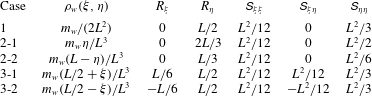
Various wing-mass distributions
 $\unicode[STIX]{x1D70C}_{w}(\unicode[STIX]{x1D709},\unicode[STIX]{x1D702})$
and their integral forms
 $R_{\unicode[STIX]{x1D709}}$
,
 $R_{\unicode[STIX]{x1D702}}$
,
 $\unicode[STIX]{x1D61A}_{\unicode[STIX]{x1D709}\unicode[STIX]{x1D709}}$
,
 $\unicode[STIX]{x1D61A}_{\unicode[STIX]{x1D709}\unicode[STIX]{x1D702}}$
and
 $\unicode[STIX]{x1D61A}_{\unicode[STIX]{x1D702}\unicode[STIX]{x1D702}}$
.
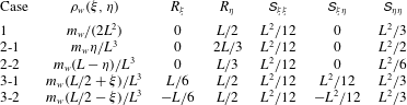
In the present study, we investigate the effects of not only the wing-mass ratio
 $\text{W}\text{R}$
but also the wing-mass distribution
 $\unicode[STIX]{x1D70C}_{w}$
. The effect of the wing-mass distribution is represented as the integral forms (2.3)–(2.7). Therefore, we consider some sets of these parameters. The cases considered here are listed in table 2. In Case 1, the mass is uniform over the wings. In Cases 2-1 and 2-2, the mass is distributed linearly in the span direction, and the wing tip is heavier in the former case, whereas the wing root is heavier in the latter case. In Cases 3-1 and 3-2, the mass is distributed linearly in the chord direction and the leading edge is heavier in the former case, whereas the trailing edge is heavier in the latter case. The wing-mass distribution of various butterflies has been measured by Betts & Wootton (Reference Betts and Wootton1988) and Dudley (Reference Dudley1990) in the form of the radius of the first and second moment of wing mass. However, their results are not enough to reproduce all the parameters given by (2.3)–(2.7). We could not find a detailed wing-mass distribution of butterfly wings, whereas Lin et al. (Reference Lin, Zheng, Hedrick and Mittal2012) reported that the wing root and the leading edge are heavier due to the concentration of large veins. Indeed, all the cases listed in table 2 are not realistic for actual butterflies. However, they cover typical cases which enable us to predict the result for an arbitrary wing-mass distribution. Therefore, the studies for these cases will give basic data for understanding the free flight of butterflies and for designing insect-inspired MAVs.
5 Results and discussion
We investigate the effects of the wing-mass ratio
 $\text{W}\text{R}$
and of the wing-mass distribution
 $\unicode[STIX]{x1D70C}_{w}$
on the free flight of the butterfly-like model. At first, we investigate Case 1 shown in table 2 for various
 $\text{W}\text{R}$
values. Then, we evaluate the difference between the cases with various
 $\unicode[STIX]{x1D70C}_{w}$
values shown in table 2.
5.1 Effect of wing-mass ratio
 $\text{W}\text{R}$

Here we investigate the effect of
 $\text{W}\text{R}$
for Case 1, i.e. the mass is uniform over the wings. At first, we calculate the inertial force and torque and compare them with the aerodynamic force and torque when the body of the model is fixed. In addition, we discuss an appropriate parameter space for free-flight simulations. Then, we calculate free flight of the model without/with rotation for various
 $Re$
and
 $\text{W}\text{R}$
values.
5.1.1 First estimation of inertial force and torque when the body is fixed
In this calculation, although the governing non-dimensional parameter is only the Reynolds number
 $Re$
for computing the aerodynamic force and torque, we need to set the non-dimensional total mass
 $N_{M}$
and the wing-mass ratio
 $\text{W}\text{R}$
to calculate the inertial force and torque given by (A 7)–(A 9). We set
 $Re=1190$
,
 $N_{M}=3.36$
and
 $0\leqslant \text{W}\text{R}\leqslant 1$
. The values of
 $Re$
and
 $N_{M}$
correspond to those for a small butterfly (Janatella leucodesma) reported by Dudley (Reference Dudley1990), and the range of
 $\text{W}\text{R}$
values covers all the possible values of
 $\text{W}\text{R}$
. Note that the wing-mass ratio of actual butterflies is typically
 $\text{W}\text{R}\simeq 0.1$
.
We define the vertical force coefficient
 $C_{L}$
, the horizontal force coefficient
 $C_{T}$
and the pitching moment coefficient
 $C_{M}$
as follows:
 $$\begin{eqnarray}\displaystyle & \displaystyle C_{L}=\frac{F_{y}}{0.5\unicode[STIX]{x1D70C}_{f}U_{tip}^{2}(2L^{2})}, & \displaystyle\end{eqnarray}$$
 $$\begin{eqnarray}\displaystyle & \displaystyle C_{T}=\frac{F_{x}}{0.5\unicode[STIX]{x1D70C}_{f}U_{tip}^{2}(2L^{2})}, & \displaystyle\end{eqnarray}$$
 $$\begin{eqnarray}\displaystyle & \displaystyle C_{M}=\frac{T_{z}}{0.5\unicode[STIX]{x1D70C}_{f}U_{tip}^{2}(2L^{3})}. & \displaystyle\end{eqnarray}$$
We put the superscript ‘in’ or ‘aero’ in the above coefficients to denote the inertial force and torque (
 $C_{L}^{in}$
,
 $C_{T}^{in}$
and
 $C_{M}^{in}$
) and to denote the aerodynamic force and torque (
 $C_{L}^{aero}$
,
 $C_{T}^{aero}$
and
 $C_{M}^{aero}$
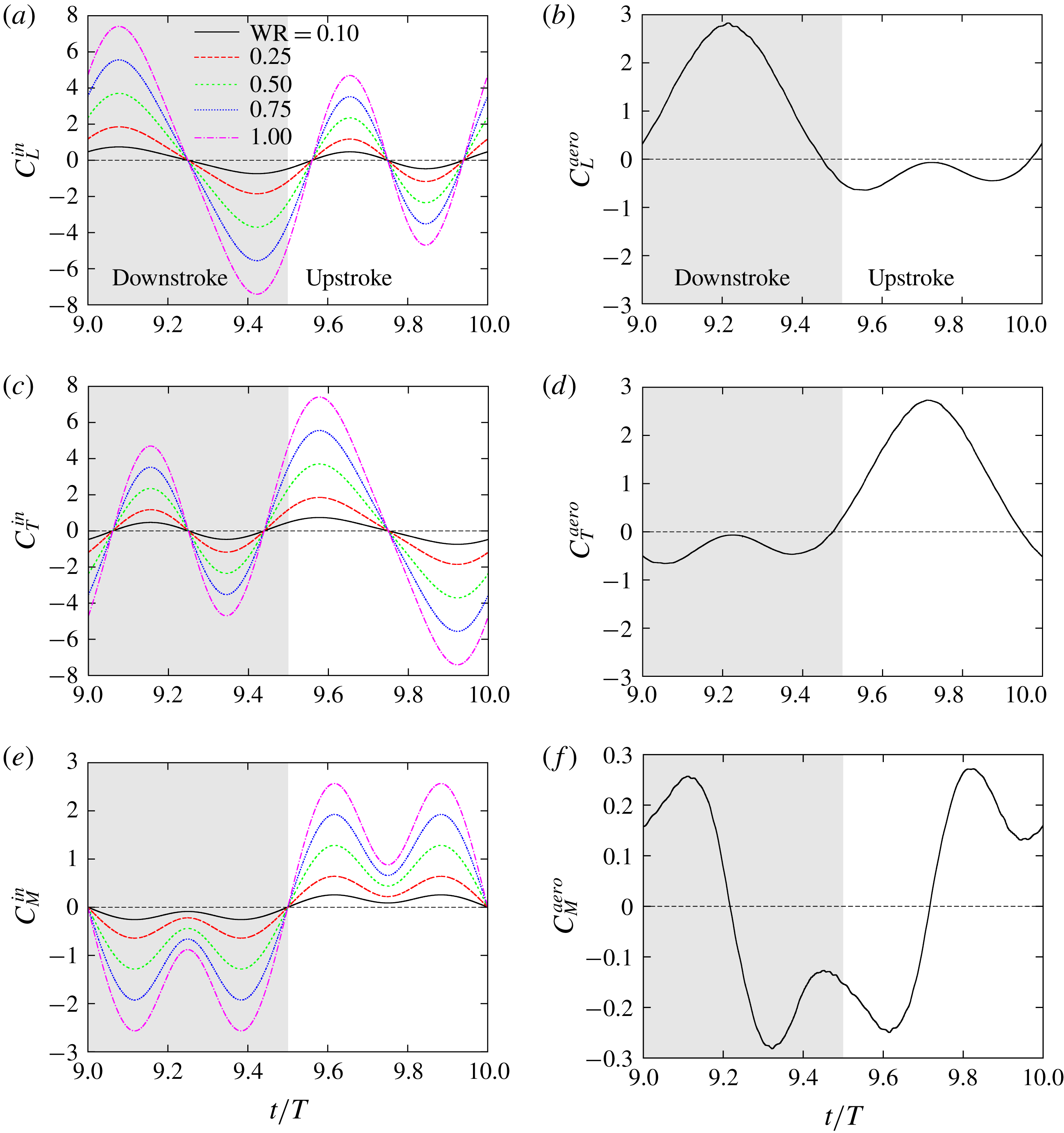
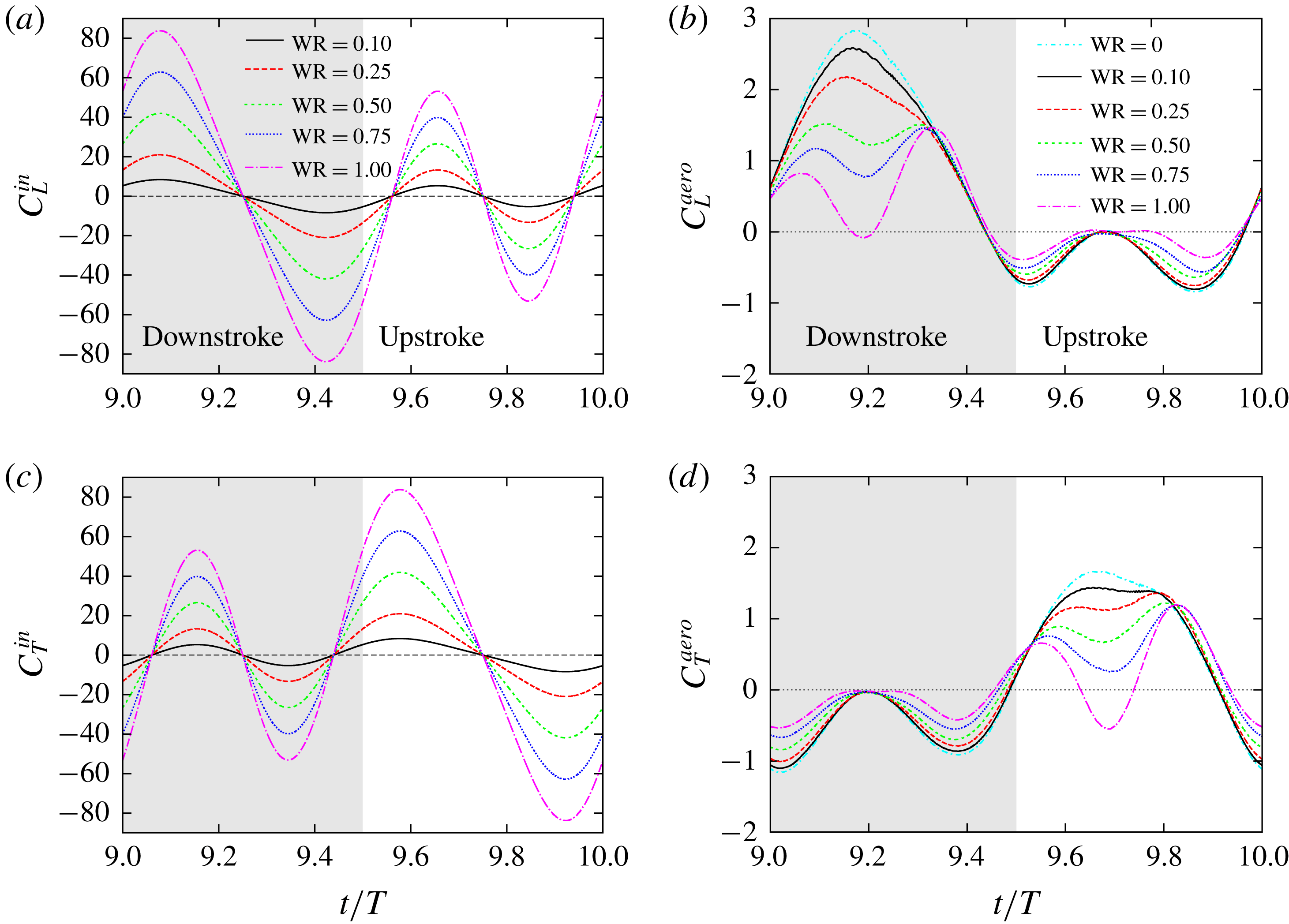
), respectively. Figure 4 shows the time variations of
 $C_{L}$
,
 $C_{T}$
and
 $C_{M}$
for the inertial and aerodynamic forces and torques in the tenth period (
 $9.0\leqslant t/T\leqslant 10.0$
). The inertial force and torque are exactly periodic after
 $t=T$
, while the aerodynamic force and torque during each stroke are almost the same after
 $t=9T$
. Thus, we present the results for the tenth stroke here.
Time variations of the vertical force, horizontal force and pitching moment coefficients
 $C_{L}$
,
 $C_{T}$
and
 $C_{M}$
for (a) the inertial force and torque and (b) the aerodynamic force and torque when the body of the model is fixed and when the Reynolds number
 $Re=1190$
and the non-dimensional total mass
 $N_{M}=3.36$
.

It can be seen from figure 4(a) that the inertial force-induced vertical force coefficient
 $C_{L}^{in}$
has large positive and negative peaks in the downstroke and has relatively small positive and negative peaks in the upstroke. The positive and negative peaks have the same magnitude. The inertial force-induced horizontal force coefficient
 $C_{T}^{in}$
is shifted by
 $T/2$
relative to
 $C_{L}^{in}$
. In addition, we can see that the inertial force-induced pitching moment coefficient
 $C_{M}^{in}$
has two large negative peaks in the downstroke and has two large positive peaks in the upstroke with the same magnitude as those in the downstroke. We can find common features in
 $C_{L}^{in}$
,
 $C_{T}^{in}$
and
 $C_{M}^{in}$
: the magnitude of the peaks proportionally increases with
 $\text{W}\text{R}$
and their time-averaged values in one period vanish. The former feature can be understood from the detailed forms of
 $F_{in\,x}$
,
 $F_{in\,y}$
and
 $T_{in}$
given by (A 7)–(A 9). They are clearly proportional to
 $m_{w}$
, and therefore their non-dimensional forms are proportional to the non-dimensional mass of the wings, i.e.
 $\text{W}\text{R}\times N_{M}$
. The latter feature is physically obvious because the friction between the wings and the body is neglected. Actually, the integrals of (A 7)–(A 9) over one period vanish.
On the other hand, it can be seen from figure 4(b) that the aerodynamic vertical force coefficient
 $C_{L}^{aero}$
has a large positive peak in the downstroke and has two small negative peaks in the upstroke. The aerodynamic horizontal force coefficient
 $C_{T}^{aero}$
is shifted by
 $T/2$
relative to
 $C_{L}^{aero}$
. This is because with
 $\unicode[STIX]{x1D6FC}_{m}=90^{\circ }$
the roles of the downstroke and the upstroke in the vertical force coefficient are equivalent to the upstroke and the downstroke in the horizontal force coefficient, respectively. In addition, we can see that the aerodynamic pitching moment coefficient
 $C_{M}^{aero}$
has positive and negative peaks which have almost the same magnitude in the downstroke, and that the curve of
 $C_{M}^{aero}$
in the upstroke looks like an inverted version of that in the downstroke, i.e.
 $C_{M}^{aero}(t)=-C_{M}^{aero}(t-T/2)$
. This is due to the symmetry of the curves of
 $C_{L}^{aero}$
and
 $C_{T}^{aero}$
. The relationship between the aerodynamic force and the vortex structure on the wings has been explained in detail by Suzuki & Yoshino (Reference Suzuki and Yoshino2018).
By comparing figures 4(a) and 4(b), it can be seen that for
 $\text{W}\text{R}=0.1$
the magnitudes of the inertial force-induced force coefficients
 $C_{L}^{in}$
and
 $C_{T}^{in}$
are about one order smaller than those of the aerodynamic force coefficients
 $C_{L}^{aero}$
and
 $C_{T}^{aero}$
, respectively, whereas for
 $\text{W}\text{R}\geqslant 0.25$
the magnitudes of
 $C_{L}^{in}$
and
 $C_{T}^{in}$
are comparable to those of
 $C_{L}^{aero}$
and
 $C_{T}^{aero}$
. In addition, we can see that even for
 $\text{W}\text{R}=0.1$
the magnitude of the inertial force-induced pitching moment coefficient
 $C_{M}^{in}$
is comparable to that of the aerodynamic pitching moment coefficient
 $C_{M}^{aero}$
, and for
 $\text{W}\text{R}\geqslant 0.25$
the magnitude of
 $C_{M}^{in}$
is much larger than that of
 $C_{M}^{aero}$
. These results suggest that the inertial force should have a significant effect on the translational motion of the body for
 $\text{W}\text{R}\geqslant 0.25$
, and the inertial torque should have a dominant effect on the rotational motion of the body even for
 $\text{W}\text{R}\geqslant 0.1$
in free flight.
5.1.2 Parameter space for free flight
In this section, we discuss an appropriate parameter space for free-flight simulations. Since there are still many governing non-dimensional parameters (
 $Re$
,
 $Fr$
,
 $N_{M}$
and
 $\text{W}\text{R}$
) in free-flight simulations, we cannot explore the entire parameter space. Therefore, we restrict the parameter space appropriately.
As explained in § 3.2, the wing length
 $L$
can be treated as equivalent to the ratio of the Reynolds number to the Froude number. In the present study, we set
 $L=3.00$
, 6.00 and 10.0 mm, and consequently
 $Fr/Re=2.94\times 10^{-2}$
,
 $1.04\times 10^{-2}$
and
 $4.83\times 10^{-3}$
. This range of
 $L$
covers scales from that of a fruit fly to that of a group of the smallest butterflies, and the results for this range of
 $L$
enable us to predict the results for larger scales.
On the other hand, the non-dimensional total mass
 $N_{M}$
can be chosen independently of
 $Re$
. In free-flight simulations, it is important to consider the situation where the total mass can be supported by the aerodynamic vertical force. Therefore, as a representative value of
 $N_{M}$
, we use the non-dimensional expected supportable total mass (Suzuki et al.
Reference Suzuki, Minami and Inamuro2015), which is estimated by the time-averaged vertical force obtained when the body of the model is fixed. The non-dimensional expected supportable total mass
 $N_{Mexp}$
is given by
 $$\begin{eqnarray}N_{Mexp}=\frac{U_{tip}^{2}}{LG}\,\overline{C_{L}^{aero}}=\left(\frac{Fr}{Re}\right)^{2}Re^{2}\,\overline{C_{L}^{aero}},\end{eqnarray}$$
where
 $\overline{C_{L}^{aero}}$
is the time-averaged aerodynamic vertical force coefficient averaged in the tenth period (
 $9.0\leqslant t/T\leqslant 10.0$
). It should be noted that
 $N_{Mexp}$
is a function of
 $Re$
and
 $L$
, since
 $\overline{C_{L}^{aero}}$
is obtained by the simulations when the body of the model is fixed, i.e.
 $\overline{C_{L}^{aero}}$
is determined only by
 $Re$
.
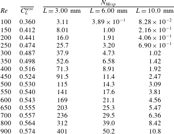
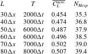
The time-averaged aerodynamic vertical force coefficient
 $\overline{C_{L}^{aero}}$
and the corresponding non-dimensional expected supportable total mass
 $N_{Mexp}$
for various
 $Re$
and
 $L$
are shown in table 3. It is noted that
 $\overline{C_{L}^{aero}}$
in table 3 is obtained when the domain size is
 $12L\times 6L\times 6L$
. As mentioned in § 4, the previous study by Suzuki et al. (Reference Suzuki, Minami and Inamuro2015) showed that the aerodynamic forces obtained when the domain size was
 $12L\times 6L\times 6L$
were almost the same as those obtained when the domain size was
 $12L\times 12L\times 12L$
. Hereafter, in order to reduce the computational cost, we will simulate free flights of the butterfly-like model for various
 $Re$
,
 $L$
and
 $\text{W}\text{R}$
by using the set of parameters listed in table 3.
The time-averaged aerodynamic vertical force coefficient
 $\overline{C_{L}^{aero}}$
in the tenth stroke when the body of the model is fixed, and the non-dimensional expected supportable total mass
 $N_{Mexp}$
for
 $L=3.00$
, 6.00 and 10.0 mm for various values of the Reynolds number
 $Re$
.

5.1.3 Free-flight simulations
We simulate the free flight of the butterfly-like model without rotation, i.e. we solve (3.8) only for
 $x_{b}$
and
 $y_{b}$
, and we set
 $\unicode[STIX]{x1D703}_{p}=\text{const.}=0^{\circ }$
. This means that the body of the model does not rotate in any direction. From a physical viewpoint, this means that the inertia moment of the body is assumed to be infinitely large, while the mass of the model is finite. Otherwise, the attitude control is assumed to be perfectly achieved and to have no effect on the translational motion of the body. The aim of this simulation is to investigate the effect of wing mass only on the translational motion of the model. In the following simulations we change the wing-mass ratio
 $\text{W}\text{R}$
while fixing the non-dimensional total mass
 $N_{M}$
. For example,
 $\text{W}\text{R}=0.1$
means that the non-dimensional mass of the wings is
 $0.1N_{M}$
and that of the body is
 $0.9N_{M}$
.
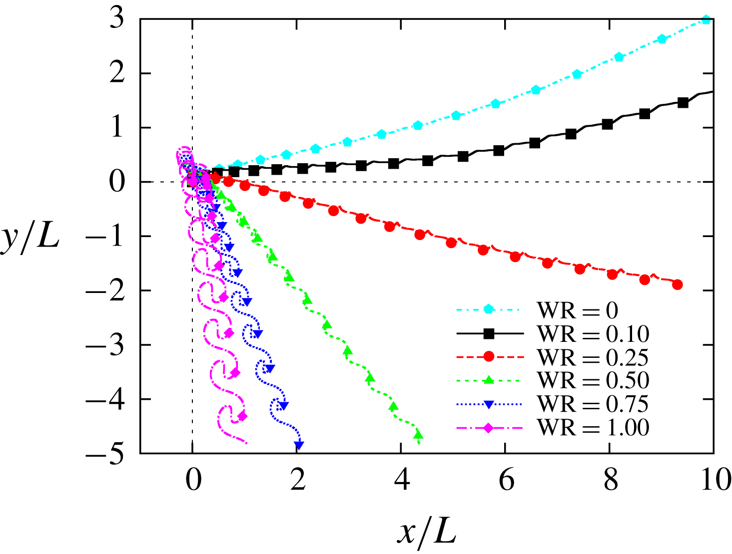
Figure 5 shows the trajectories of the centre of the body for various wing-mass ratios
 $\text{W}\text{R}$
when
 $Re=300$
and
 $L=3.00$
mm, i.e. the scale of a fruit fly. In this simulation, we set
 $N_{M}=N_{Mexp}=37.9$
as shown in table 3. Note that the total mass of the model can be supported by the aerodynamic vertical force obtained when the body of the model is fixed. We can see from figure 5 that for
 $\text{W}\text{R}\leqslant 0.10$
the model can go upward against gravity, whereas for
 $\text{W}\text{R}\geqslant 0.25$
it goes downward. This means that a large wing-mass ratio reduces the aerodynamic force during the translational motion of the model.
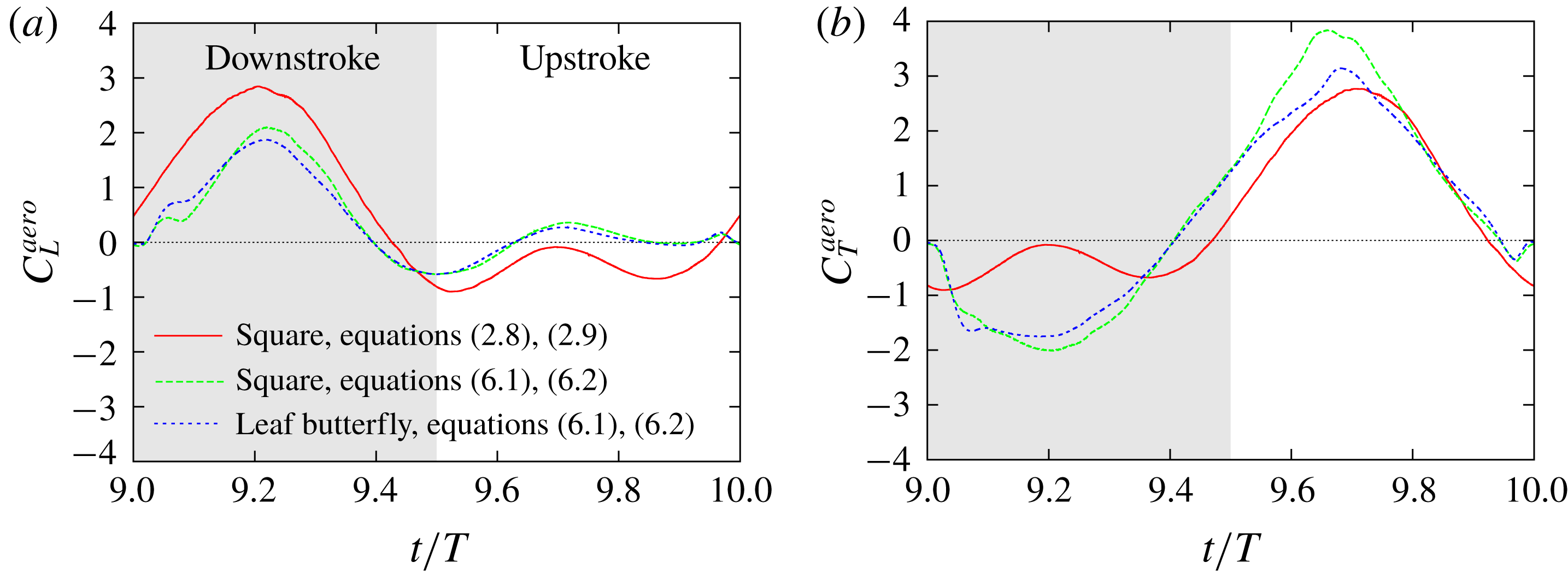
This effect can be found more clearly in the time variations of the vertical and horizontal force coefficients shown in figure 6. We can see from figure 6(a) that the inertial forces have the same tendency as those shown in figure 4(a) when the body of the model is fixed, whereas their magnitudes in figure 6(a) are much larger than those in figure 4(a). This is because the inertial forces (A 7) and (A 8) do not include any information about the translational motion of the body, and their non-dimensional forms are proportional to
 $\text{W}\text{R}\times N_{M}$
. On the other hand, it can be seen from figure 6(b) that the positive peaks of both
 $C_{L}^{aero}$
and
 $C_{T}^{aero}$
decrease clearly with
 $\text{W}\text{R}$
. Therefore, we can predict a scenario in which as
 $\text{W}\text{R}$
increases, the magnitudes of the inertial forces increase, the body motion is affected by the inertial forces and then the aerodynamic forces are weakened due to the body motion.
The trajectories of the centre of the body for various wing-mass ratios
 $\text{W}\text{R}$
(
 $L=3.00$
mm,
 $Re=300$
). The symbols on the trajectories indicate the position of the centre of the body when the wings are at
 $\unicode[STIX]{x1D703}=\unicode[STIX]{x1D703}_{m}$
.

Time variations of the vertical and horizontal force coefficients
 $C_{L}$
and
 $C_{T}$
for (a) the inertial force and (b) the aerodynamic force in free flight without rotation when the wing length
 $L=3.00$
mm and the Reynolds number
 $Re=300$
.

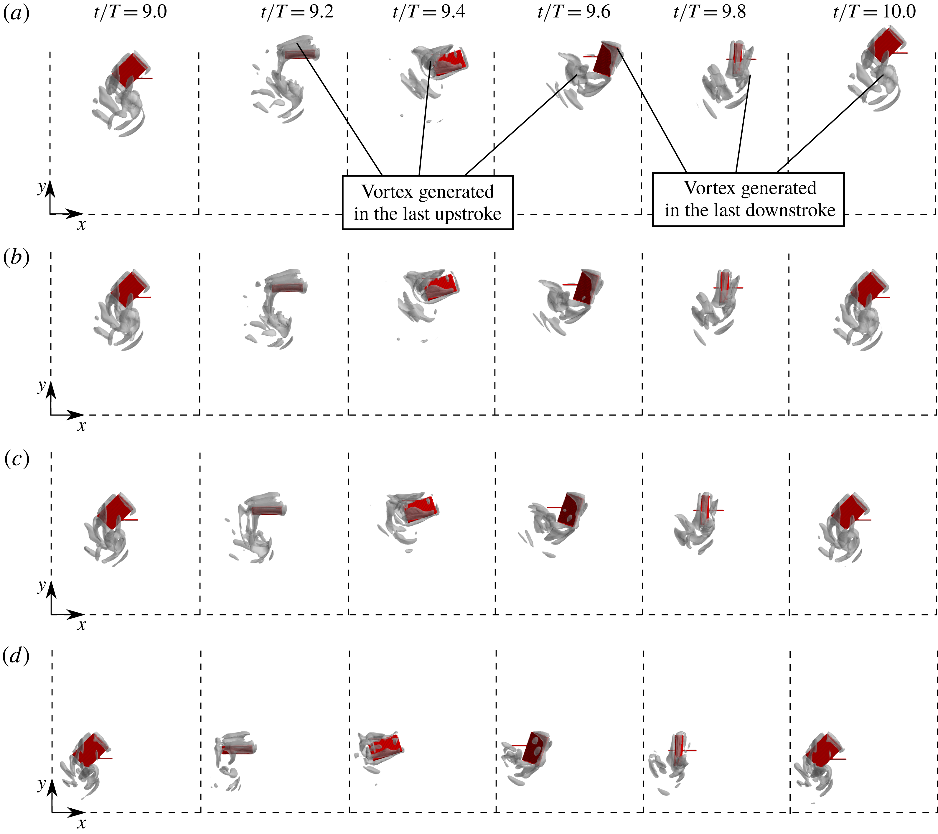
Snapshots of the model and the vortex around it viewed from its right-hand side at various values of
 $t/T$
for
 $\text{W}\text{R}=$
(a) 0.00, (b) 0.10, (c) 0.25 and (d) 0.50 in free flight without rotation when the wing length
 $L=3.00$
mm and the Reynolds number
 $Re=300$
. The vortex is shown by the isosurface of
 $Q=10(U_{tip}/L)^{2}$
. It should be noted that all the frames in this figure show the same region of the computational domain.

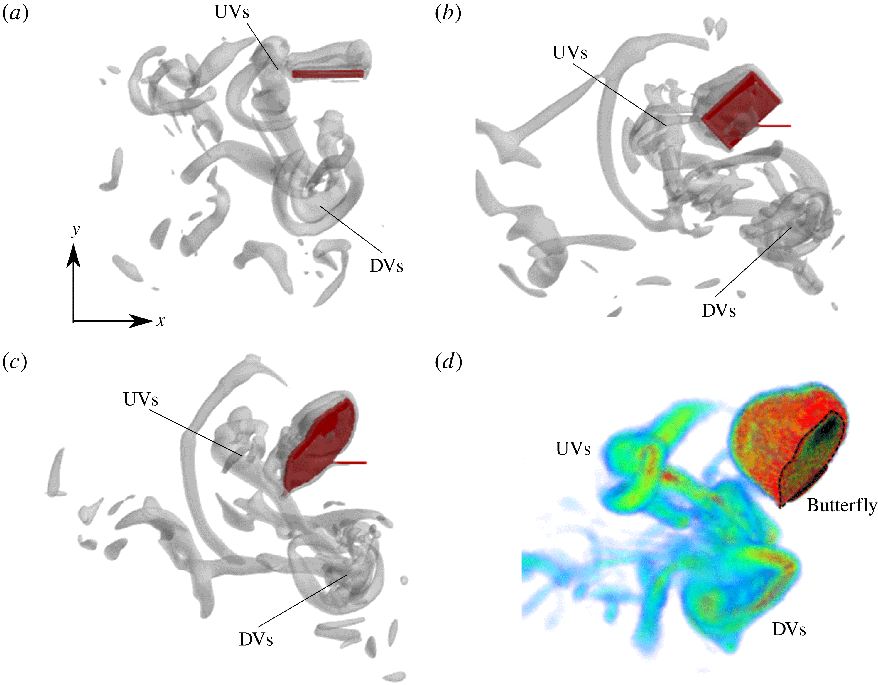
In order to discuss how the aerodynamic forces are weakened, we observe the vortex structures around the model. Figure 7 shows snapshots of the model and the vorticity around it in the tenth stroke when
 $\text{W}\text{R}=0.00$
, 0.10, 0.25 and 0.50. The vortex structure is visualized by the
 $Q$
-criterion (Hunt, Wray & Moin Reference Hunt, Wray and Moin1988), i.e. the second invariant of the velocity gradient tensor given by
 $$\begin{eqnarray}Q=-\frac{\unicode[STIX]{x2202}u_{i}}{\unicode[STIX]{x2202}x_{j}}\frac{\unicode[STIX]{x2202}u_{j}}{\unicode[STIX]{x2202}x_{i}},\end{eqnarray}$$
where
 $i,j=x,y,z$
represent the Cartesian coordinates and the summation convention is used. The
 $Q$
-criterion identifies low-pressure vortex structures. We can see from this figure that the vortices generated in the last downstroke are released downward and those generated in the last upstroke are released backward, which can be observed in the free flight of actual butterflies (Yokoyama et al.
Reference Yokoyama, Senda, Iima and Hirai2013; Fei & Yang Reference Fei and Yang2015; Fuchiwaki & Tanaka Reference Fuchiwaki and Tanaka2016). Although the model goes upward when
 $\text{W}\text{R}=0.00$
and 0.10, it goes downward when
 $\text{W}\text{R}=0.25$
and 0.50. In addition, we can see that the vortices weaken with increasing
 $\text{W}\text{R}$
. This is not only because the distance travelled by the model decreases with increasing
 $\text{W}\text{R}$
as shown in figure 5, but also because the generated vortex itself weakens.
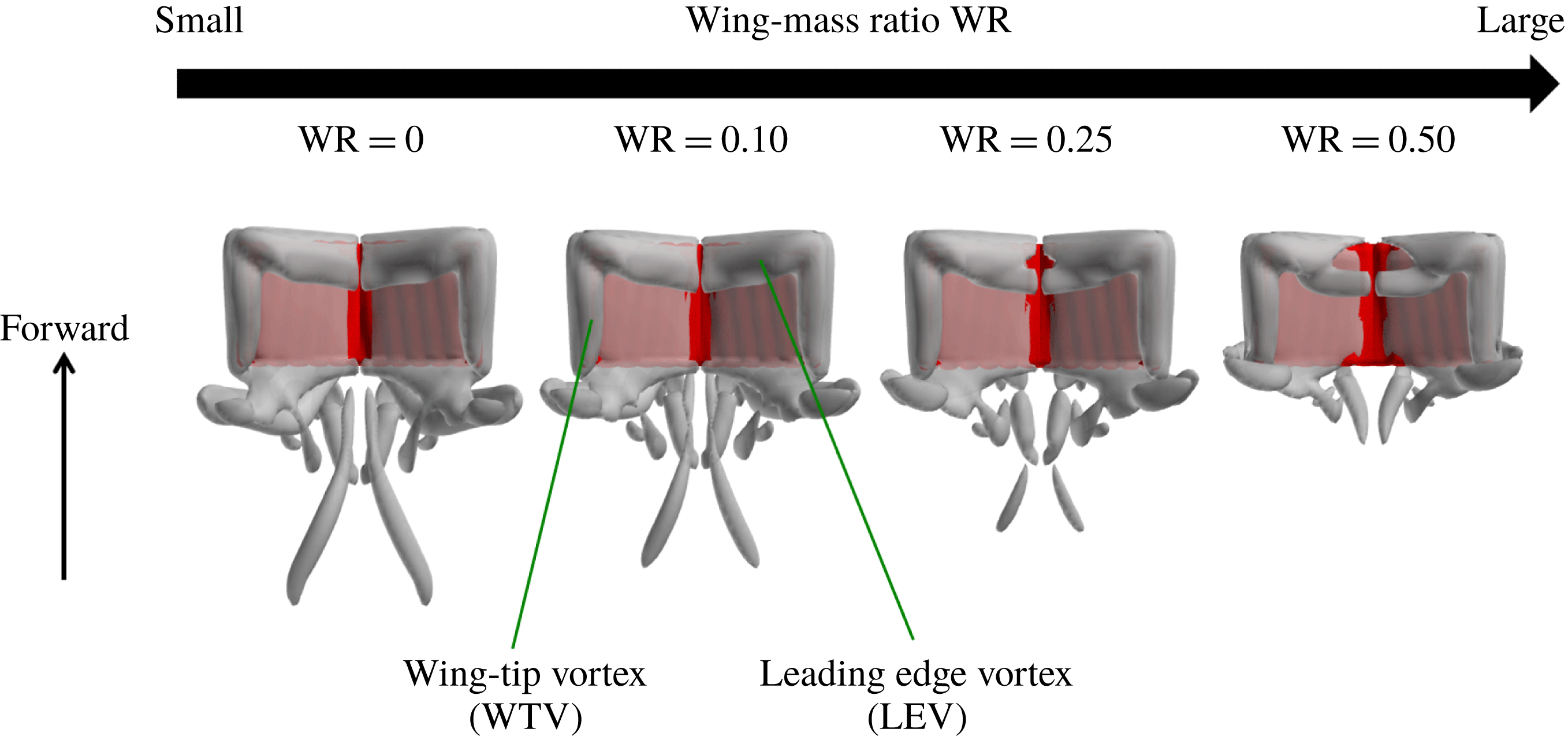
Such weakening of the vortex can be observed in the vortex structures on the wings in the downstroke. Figure 8 shows the vortex structures on the wings visualized by the
 $Q$
-criterion at
 $t/T=9.2$
, i.e. when the aerodynamic vertical force coefficient
 $C_{L}^{aero}$
has its positive peak. We can see that the wing-tip vortex (WTV) and the leading-edge vortex (LEV) appear on the upper surface of the wings, and they are connected at the corner of the wings. Like an actual butterfly, the WTV and the LEV are considered to be a major cause of the lift and thrust generation of the present model. For a large
 $\text{W}\text{R}$
, however, the part of the leading edge near the wing root is not covered by the LEV. This induces a decrease of the aerodynamic vertical force at this time, which is consistent with the result shown in figure 6(b). The reason why the generated vortices weaken with increasing
 $\text{W}\text{R}$
is explained as follows. For a large
 $\text{W}\text{R}$
, the body goes up and down (back and forth) over a large distance due to the large inertial force-induced vertical (horizontal) force during each stroke. This can be seen especially in the trajectory for
 $\text{W}\text{R}=1.00$
shown in figure 5. Thus, the speeds of the leading edge and the wing tip relative to the coordinate system of the flight space are likely to decrease. Consequently, the WTV and the LEV weaken. Since the speed relative to the coordinate system of the flight space is especially small in the part of the leading edge near the wing root, the LEV cannot be generated in this part as shown in figure 8.
Vortex structures visualized by the
 $Q$
-criterion, the second invariant of the velocity gradient tensor, at
 $t/T=9.2$
for various wing-mass ratios
 $\text{W}\text{R}$
viewed from the top side of the model in free flight without rotation when the wing length
 $L=3.00$
mm and the Reynolds number
 $Re=300$
. The vortex is shown by the isosurface of
 $Q=10(U_{tip}/L)^{2}$
.

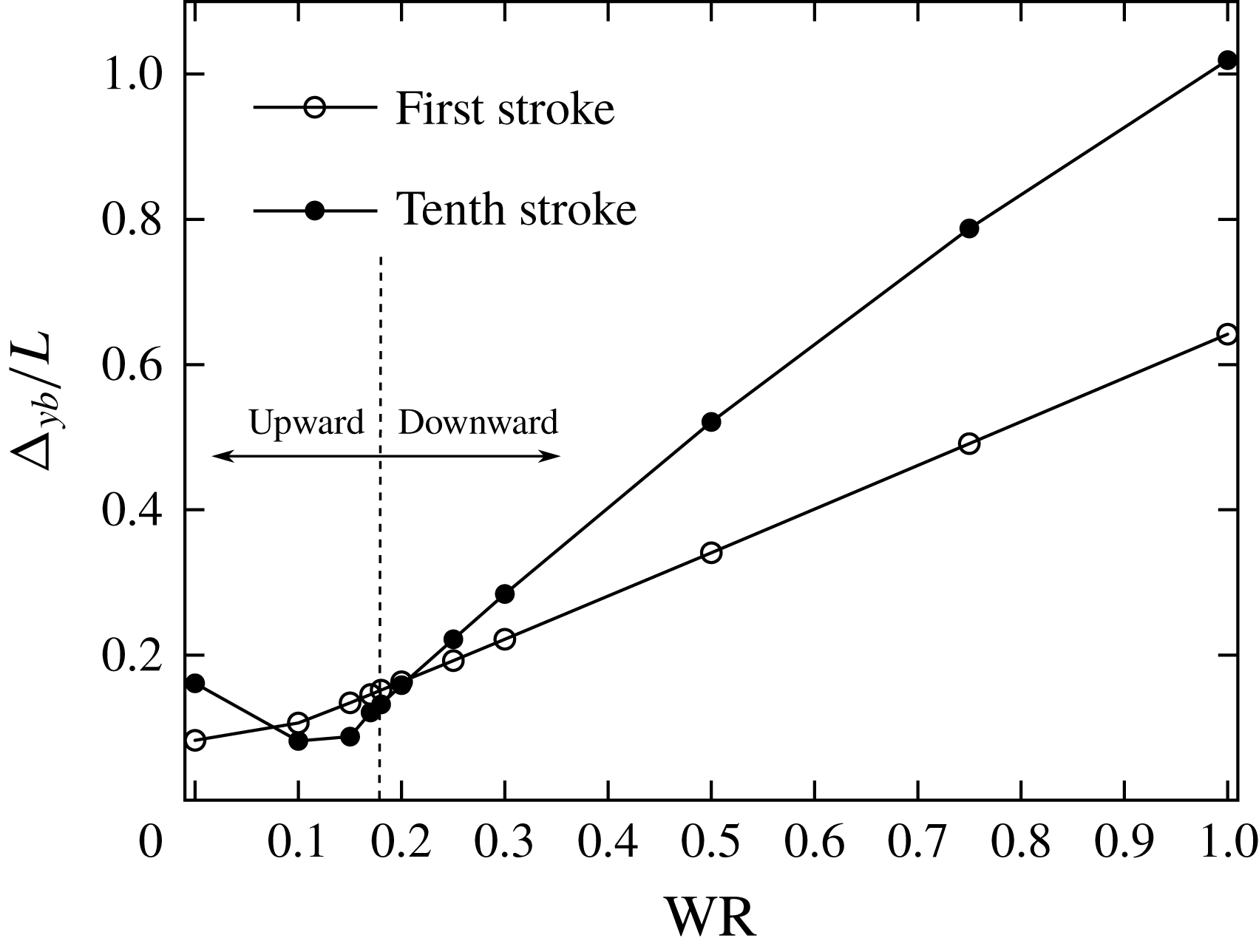
The difference
 $\unicode[STIX]{x0394}y_{b}$
between the maximum and minimum values of the vertical position
 $y_{b}$
during the first and the tenth strokes as a function of the wing-mass ratio
 $\text{W}\text{R}$
in free flight without rotation when the wing length
 $L=3.00$
mm and the Reynolds number
 $Re=300$
.

In order to show how much the body goes up and down during one stroke, we calculate the difference
 $\unicode[STIX]{x0394}y_{b}$
between the maximum and minimum values of the vertical position
 $y_{b}$
during one stroke. This difference is a measure of the amplitude of the oscillation in the body motion. Figure 9 shows the differences during the first and the tenth strokes as a function of
 $\text{W}\text{R}$
. We can see that
 $\unicode[STIX]{x0394}y_{b}$
during the first stroke increases with increasing
 $\text{W}\text{R}$
. On the other hand,
 $\unicode[STIX]{x0394}y_{b}$
during the tenth stroke decreases when
 $\text{W}\text{R}<0.1$
and increases when
 $\text{W}\text{R}>0.1$
. This is because when
 $\text{W}\text{R}<0.1$
,
 $\unicode[STIX]{x0394}y_{b}$
shows the climbing displacement rather than the amplitude of the oscillation in the body motion since the oscillation is relatively small. In addition, we can see that
 $\unicode[STIX]{x0394}y_{b}$
during the tenth stroke is larger than that during the first stroke when the model goes downward totally. This is because
 $\unicode[STIX]{x0394}y_{b}$
shows the falling displacement rather than the amplitude of the oscillation in the body motion since gravity accelerates the falling speed of the body. In any case, the body goes up and down over a larger distance during one stroke as
 $\text{W}\text{R}$
increases.
The values of the Reynolds number
 $Re$
and the wing-mass ratio
 $\text{W}\text{R}$
resulting in upward flight and downward flight when the wing length
 $L=3.00$
mm. The line indicates the critical wing-mass ratio
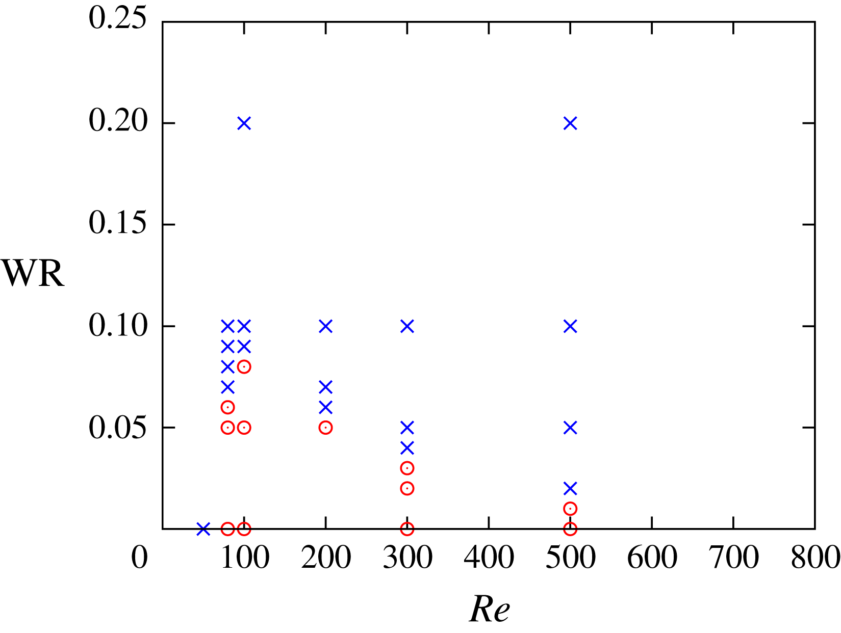
 $\text{W}\text{R}_{c}$
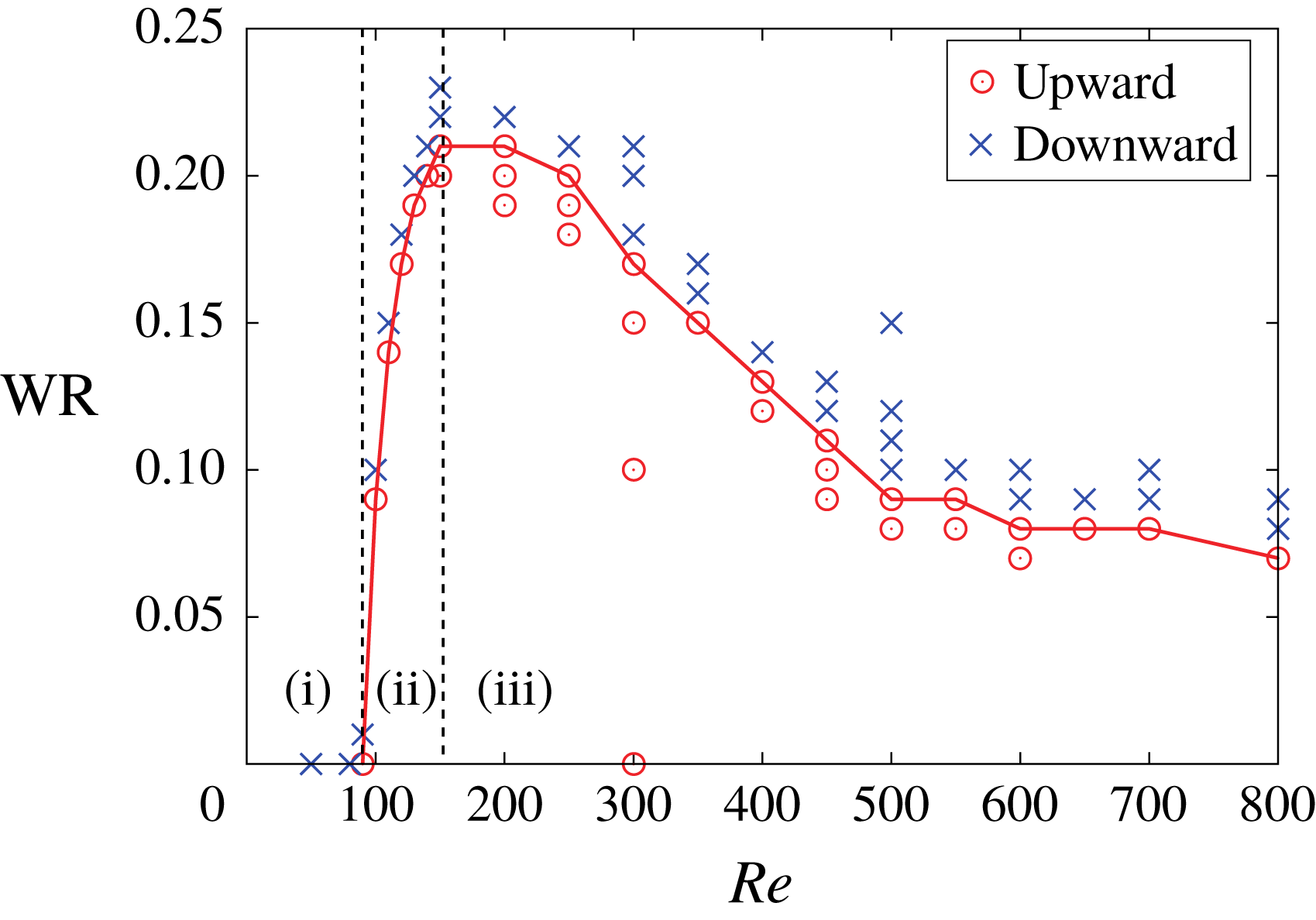
. The following three regions exist: (i)
 $\text{W}\text{R}_{c}=0$
, i.e. the model goes down even without wing mass (
 $Re<100$
), (ii)
 $\text{W}\text{R}_{c}$
steeply increases (
 $100<Re<150$
) and (iii)
 $\text{W}\text{R}_{c}$
gradually decreases (
 $150<Re$
).

From the results shown in figure 5, there is the critical value of
 $\text{W}\text{R}$
between upward and downward flights. In order to find the critical wing-mass ratio
 $\text{W}\text{R}_{c}$
, we calculate free flights for various
 $Re$
and
 $\text{W}\text{R}$
. The total mass of the model is determined in accordance with table 3. We define the upward flight and the downward flight to be when the time-averaged vertical velocity
 $V_{m}$
defined below is positive and negative, respectively,
 $$\begin{eqnarray}V_{m}=\frac{1}{t_{2}-t_{1}}\int _{t_{1}}^{t_{2}}{\dot{y}}_{b}\,\text{d}t.\end{eqnarray}$$
We take the integration interval
 $[t_{1},t_{2}]$
in (5.6) as
 $[0,20T]$
, since we focus on the take-off from the resting state and the transitional motion to the forward flight. When we focus on the forward flight, we can use a shorter integration interval, e.g.
 $[10T,20T]$
or
 $[15T,20T]$
. The discussion below is not affected by the choice of the integration interval (see appendix C). The critical wing-mass ratio
 $\text{W}\text{R}_{c}$
is defined as the maximum value of
 $\text{W}\text{R}$
resulting in the upward flight. The results for
 $L=3.00$
mm are shown in figure 10. From this figure, we can find that the following three regions in
 $\text{W}\text{R}_{c}$
exist as a function of the Reynolds number
 $Re$
: (i)
 $\text{W}\text{R}_{c}=0$
, i.e. the model goes down even without the wing mass (
 $Re<100$
), (ii)
 $\text{W}\text{R}_{c}$
steeply increases (
 $100<Re<150$
) and (iii)
 $\text{W}\text{R}_{c}$
gradually decreases (
 $150<Re$
). The mechanism of each region can be explained as follows. In region (i), the body moves up and down over a large distance due not to the inertial force but to the aerodynamic force during one stroke since the non-dimensional total mass
 $N_{M}$
is so small, and consequently the WTV and the LEV weaken for the same reason explained in the previous paragraph. In region (ii), the body motion during one stroke is suppressed due to the increase in
 $N_{M}$
, and the model can generate stronger WTV and LEV. In addition, the vertical force is enhanced by the decrease in the viscosity and by the increase in the forward speed of the body. In region (iii), the translational motion of the body is too suppressed due to the further increase in
 $N_{M}$
, and consequently its forward speed decreases. Since the enhancement of the vertical force by the forward speed is suppressed, the critical wing-mass ratio
 $\text{W}\text{R}_{c}$
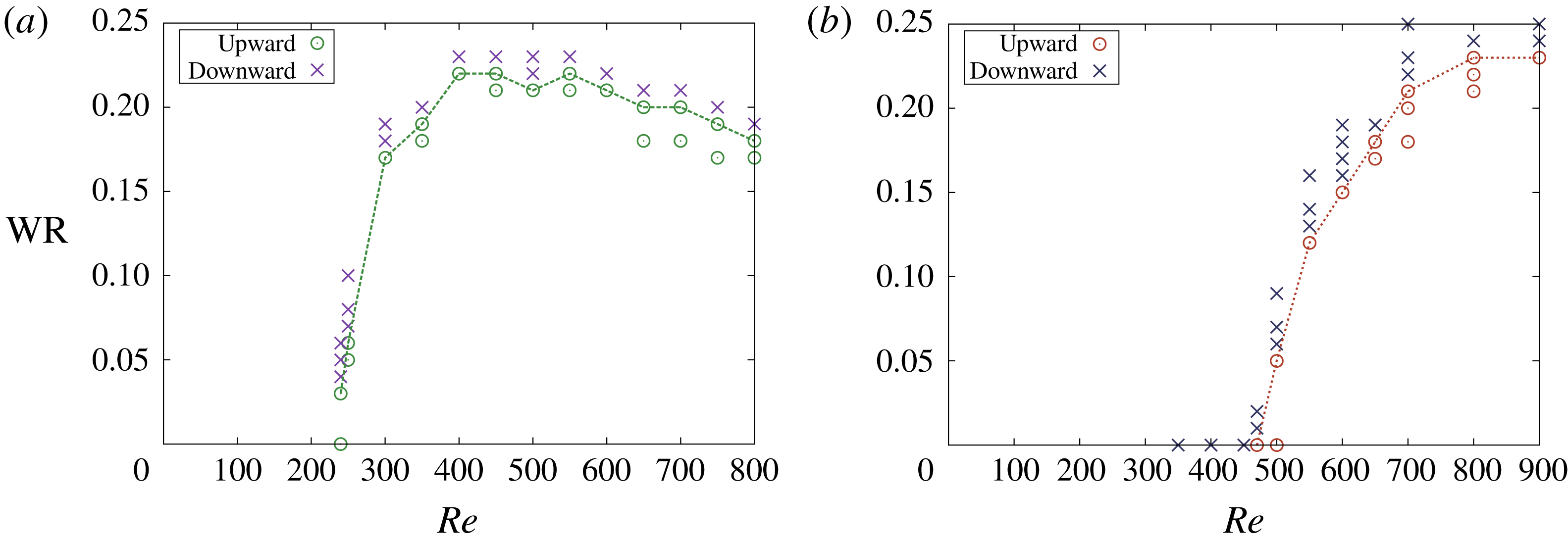
decreases. The same regions can be found in the results for
 $L=6.00$
and 10.0 mm shown in figure 11, although the ranges of these regions are different.
The values of the Reynolds number
 $Re$
and the wing-mass ratio
 $\text{W}\text{R}$
resulting in upward flight and downward flight when the wing length is (a)
 $L=6.00$
mm and (b)
 $L=10.0$
mm. The line indicates the critical wing-mass ratio
 $\text{W}\text{R}_{c}$
.

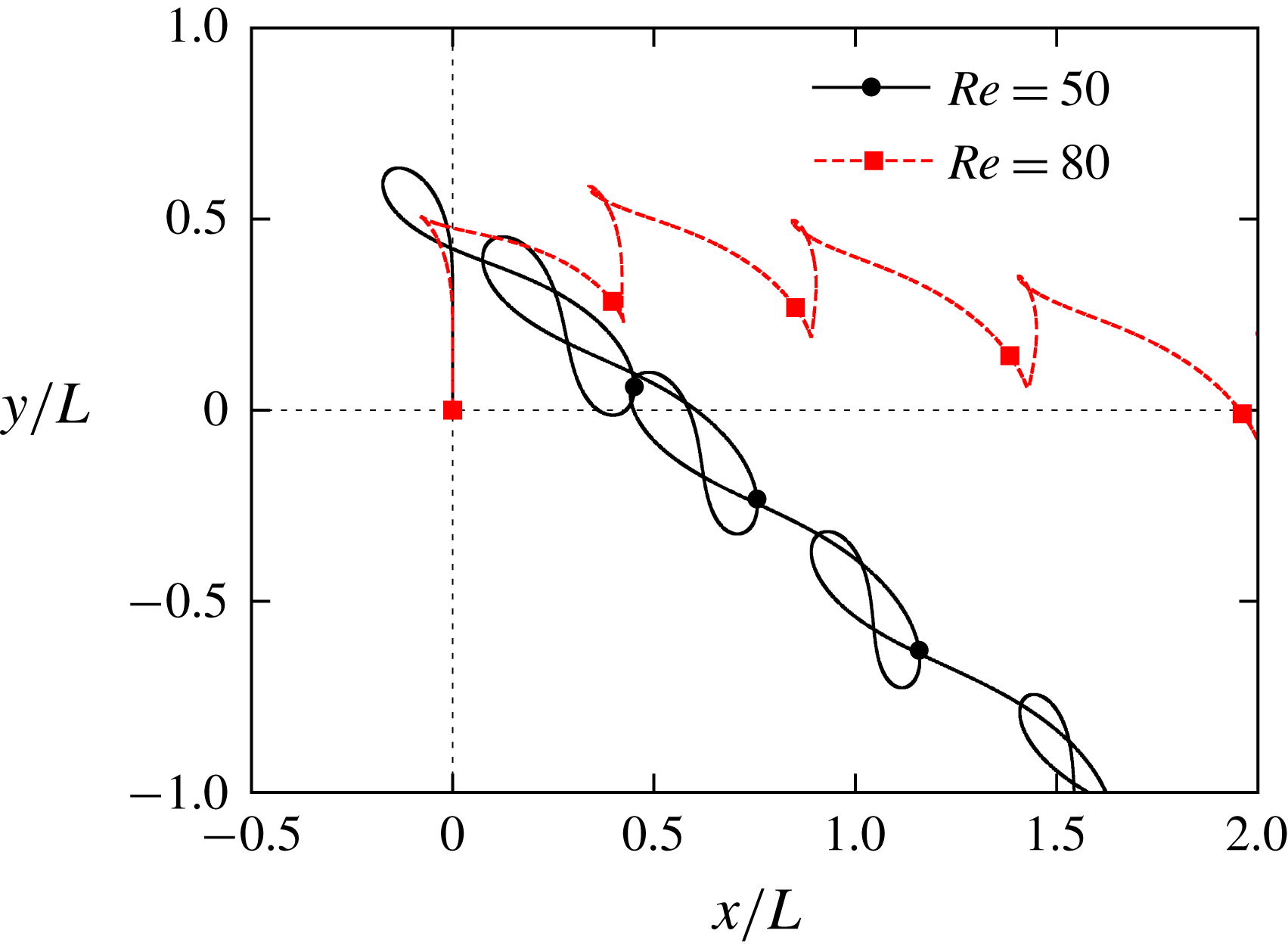
The trajectories of the centre of the body when
 $Re=50$
and 80 (
 $L=3.00$
mm and
 $\text{W}\text{R}=0.0$
). The symbols on the trajectories indicate the position of the centre of the body when the wings are at
 $\unicode[STIX]{x1D703}=\unicode[STIX]{x1D703}_{m}$
.

One might consider that the flight failure in region (i) can be caused not by the large oscillation in the body motion in transitional motion but by the inability to form vortex structures during take-off. In order to distinguish between them, we observe the trajectory at the early stage from take-off in region (i). Figure 12 shows the trajectories of the centre of the body when
 $L=3.00$
mm and
 $\text{W}\text{R}=0.0$
. We can see that the model can go upward in the first stroke. However, it goes downward averagely in the later strokes. This means that the model succeeds at take-off and then falls. We can see that the model goes up and down more as
 $Re$
decreases. This is because we use a smaller
 $N_{M}$
for a smaller
 $Re$
. Therefore, we can see that the large oscillation in the body motion in transitional motion causes the flight failure in region (i).
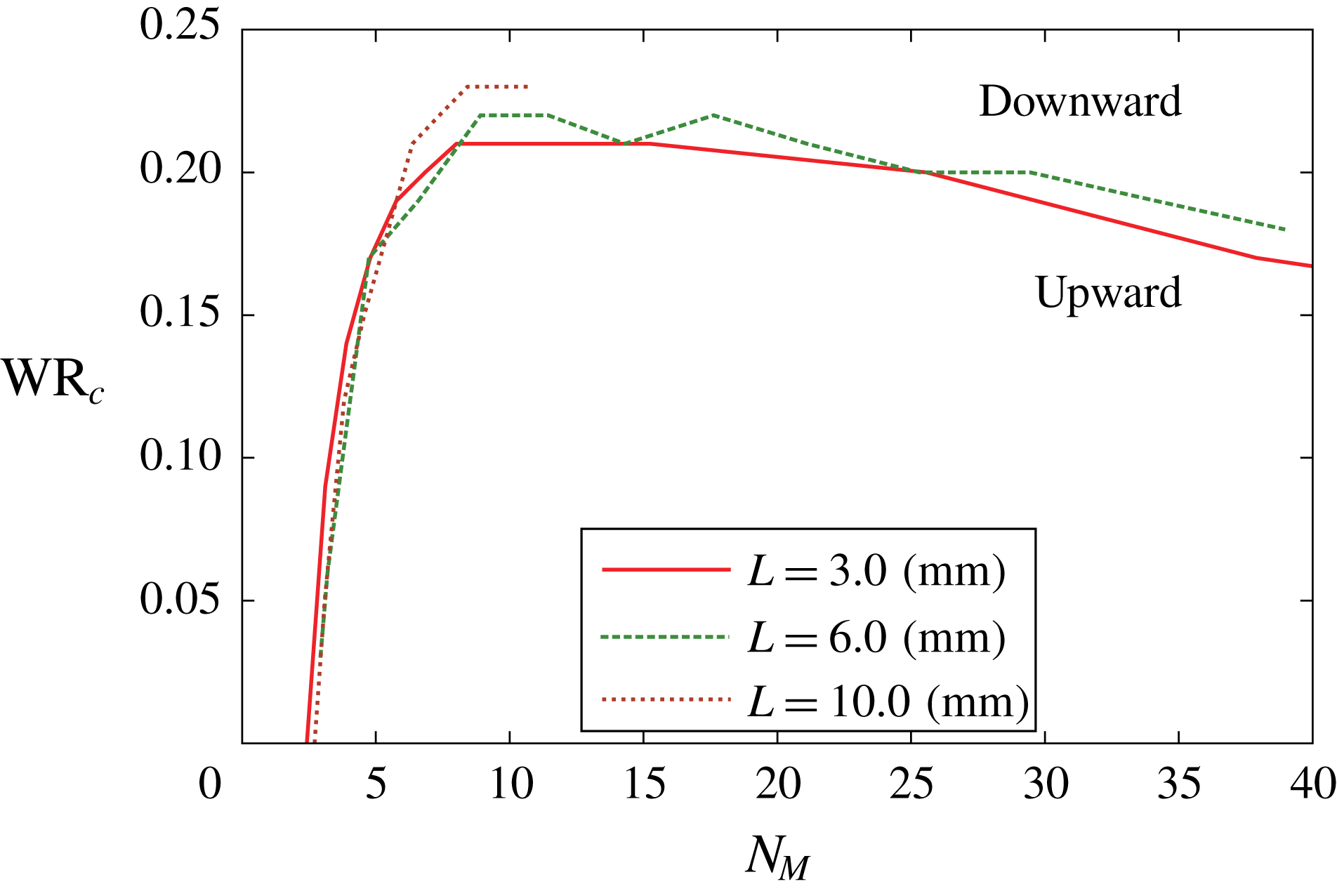
The critical wing-mass ratio
 $\text{W}\text{R}_{c}$
as a function of the non-dimensional total mass
 $N_{M}$
when the wing length is
 $L=3.00$
, 6.00 and 10.0 mm.

From the above discussion about the regions of the critical wing-mass ratio
 $\text{W}\text{R}_{c}$
, we can see that they are governed by
 $N_{M}$
rather than by
 $Re$
. Therefore, we replot the data of figures 10 and 11 in the map of
 $N_{M}$
–
 $\text{W}\text{R}$
. Figure 13 shows the curves of
 $\text{W}\text{R}_{c}$
as a function of
 $N_{M}$
when
 $L=3.00$
, 6.00 and 10.0 mm. In this figure, the areas above and below the curves correspond to the downward and upward flights, respectively. We can see from this figure that the three curves for different wing lengths are very similar in terms of the range of the three regions and the peak value of
 $\text{W}\text{R}_{c}$
. This means that the relationship between
 $\text{W}\text{R}_{c}$
and
 $N_{M}$
is almost independent of
 $L$
, whereas the relationship between
 $\text{W}\text{R}_{c}$
and
 $Re$
strongly depends on
 $L$
. Therefore, we can predict the curve of
 $\text{W}\text{R}_{c}$
as a function of
 $N_{M}$
for a larger
 $L$
from the present curves in figure 13.
In addition, we examine the effect of
 $\text{W}\text{R}$
on the rotational motion of the butterfly-like model. We simulate free flight of the model with rotation (pitching motion), i.e. we solve (3.8) fully. Therefore, the model can rotate in the pitching direction, while it does not rotate in the yawing or rolling directions. The aim of this simulation is to investigate the effect of wing mass on the pitching motion of the model in addition to the translational motion. We set
 $L=3.00$
mm,
 $Re=300$
and
 $N_{M}=37.9$
for which the model can go upward against gravity when
 $\text{W}\text{R}=0.00$
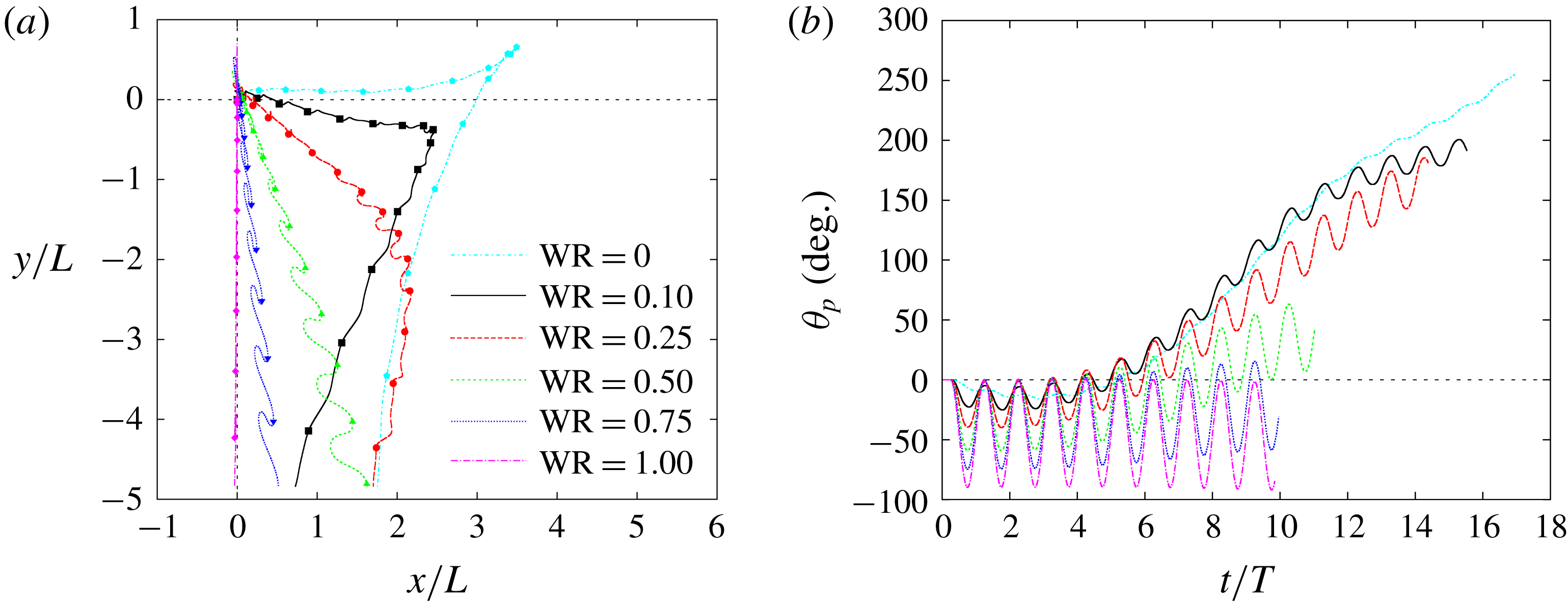
. Figure 14 shows the trajectories of the centre of the body
 $(x_{b},y_{b})$
and the time variations of the pitching angle
 $\unicode[STIX]{x1D703}_{p}$
of the body for various
 $\text{W}\text{R}$
. It can be seen from this figure that when
 $\text{W}\text{R}=0.00$
the pitching angle
 $\unicode[STIX]{x1D703}_{p}$
increases gradually, and eventually the model turns over in the same way as for the results of Suzuki et al. (Reference Suzuki, Minami and Inamuro2015). In addition, we can see that the oscillation of
 $\unicode[STIX]{x1D703}_{p}$
during one stroke increases as
 $\text{W}\text{R}$
increases, and the model goes downward from the beginning of the free flight when
 $\text{W}\text{R}\geqslant 0.10$
. Therefore,
 $\text{W}\text{R}$
has a dominant effect on the rotational motion of the model, and a large
 $\text{W}\text{R}$
reduces aerodynamic force and intensifies the time variation of the pitching angle.
(a) The trajectories of the centre of the body and (b) the time variations of the pitching angle of the body for various wing-mass ratios
 $\text{W}\text{R}$
(
 $L=3.00$
mm and
 $Re=300$
) when the model can rotate in the pitching direction. In (a), the symbols on the trajectories indicate the position of the centre of the body when the wings are at
 $\unicode[STIX]{x1D703}=\unicode[STIX]{x1D703}_{m}$
.

5.2 Effect of wing-mass distribution
$\unicode[STIX]{x1D70C}_{w}$

Second, we investigate the effect of the wing-mass distribution
 $\unicode[STIX]{x1D70C}_{w}$
. We focus on how the critical wing-mass ratio
 $\text{W}\text{R}_{c}$
as a function of
 $N_{M}$
(figure 13) changes with the wing-mass distribution. Therefore, we calculate free flights of the butterfly-like model without rotation for the wing-mass distributions listed in table 2, and we set
 $L=3.00$
mm,
 $Re=300$
and
 $N_{M}=37.9$
for which the model can go upward against gravity when
 $\text{W}\text{R}=0.00$
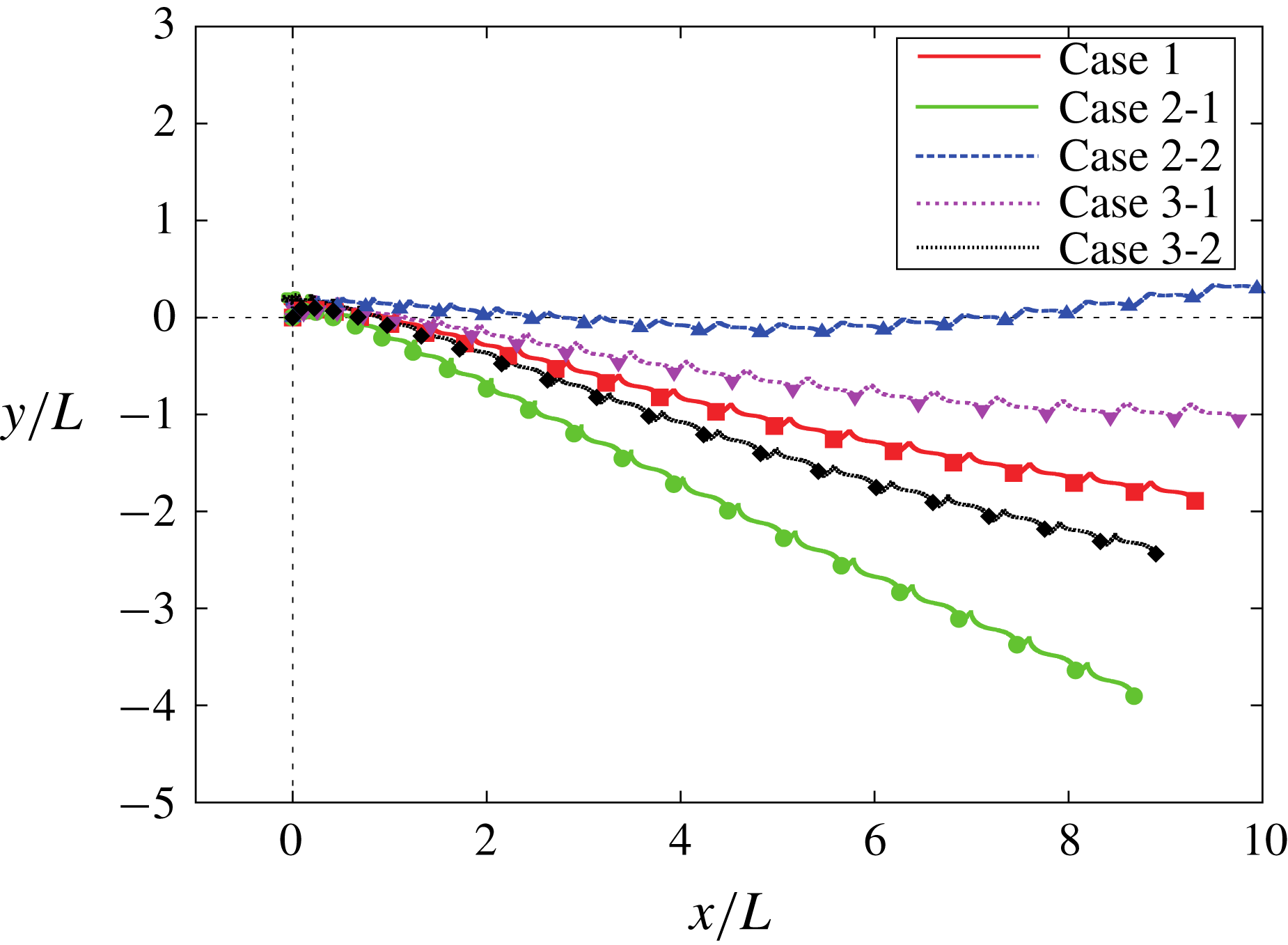
. Figure 15 shows the trajectories of the centre of the body for various cases with different wing-mass distributions when
 $\text{W}\text{R}=0.25$
. We can see that the curves for Cases 2-2 and 3-1 are above the curve for Case 1, whereas the curves for Cases 2-1 and 3-2 are below the curve for Case 1. This means that for Cases 2-2 and 3-1 the model can generate a larger vertical force than for Case 1, whereas for Cases 2-1 and 3-2 it generates a smaller vertical force than for Case 1.
The trajectories of the centre of the body for various cases with different wing-mass distributions when
 $\text{W}\text{R}=0.25$
(
 $L=3.00$
mm and
 $Re=300$
). The symbols on the trajectories indicate the position of the centre of the body when the wings are at
 $\unicode[STIX]{x1D703}=\unicode[STIX]{x1D703}_{m}$
.

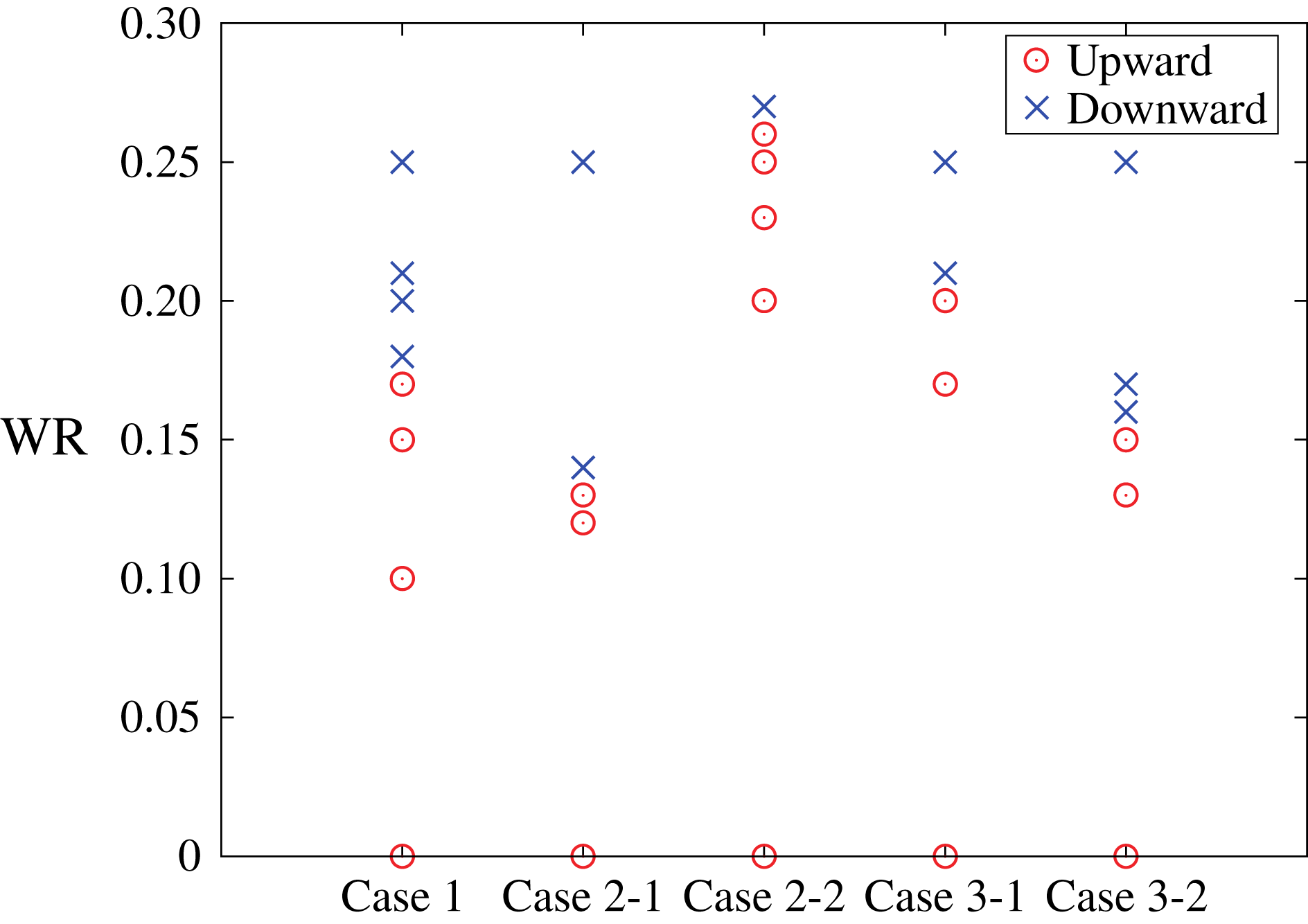
The values of the wing-mass ratio
 $\text{W}\text{R}$
resulting in upward flight and downward flight for various cases with different density distributions when the wing length
 $L=3.00$
mm and the Reynolds number
 $Re=300$
.

We can easily explain the above results for Cases 2-1 and 2-2 from the form of the inertial forces (A 7) and (A 8). In these cases, the inertial forces
 $F_{in\,x}$
and
 $F_{in\,y}$
are proportional to
 $m_{w}R_{\unicode[STIX]{x1D702}}$
since
 $R_{\unicode[STIX]{x1D709}}=0$
. The factor
 $m_{w}R_{\unicode[STIX]{x1D702}}$
for Cases 2-1 and 2-2 is
 $4/3$
and
 $2/3$
times as large as that for Case 1, respectively. In Cases 2-1 and 2-2, therefore, the wing mass
 $m_{w}$
(i.e. the wing-mass ratio
 $\text{W}\text{R}$
) is effectively larger and smaller than that for Case 1, respectively. Hence, for Case 2-2 the model can generate a larger vertical force than for Case 1, whereas for Case 2-1 it generates a smaller vertical force than for Case 1, for the same reason as explained in § 5.1.3. As for Cases 3-1 and 3-2, we cannot explain the results in the same way as for Cases 2-1 and 2-2 since
 $R_{\unicode[STIX]{x1D709}}\neq 0$
. However, we can see from figure 15 that the curves for Cases 3-1 and 3-2 are between those for Cases 2-1 and 2-2. This means that the effect of the wing-mass distribution in the chordwise direction is less than that in the spanwise direction.
We categorize the results for various
 $\text{W}\text{R}$
at
 $L=3.00$
mm and
 $Re=300$
into the upward flight and the downward flight in the five cases, and we plot the results in figure 16. We can see that the boundary between the upward and downward flights (i.e.
 $\text{W}\text{R}_{c}$
) is the largest for Case 2-2 and the smallest for Case 2-1. From the results, we can expect that the results for wings of actual butterflies and of MAVs are likely to be between those for Cases 2-1 and 2-2, since the two cases are extreme cases of possible wing-mass distributions of such actual wings.
6 Discussion: the limitations of the model
Finally, we discuss the limitations of the model. The present study will give valuable data for the design of insect-inspired MAVs. However, there are limitations in explaining the flapping flight of actual butterflies from the present results, since the present model is highly simplified in the components of the model, the wing kinematics of the model and the computational settings. We discuss the limitations of the model below.
6.1 Limitation due to the components of the model
The components of the model (§ 2.1) are simplified in terms of the following points:
(1) The wings of the model are square and their aspect ratio is 2 (defined by the ratio of the square of the wing span to the wing area of two wings), while an actual butterfly’s wings are more complicated and their aspect ratio is around 3.06 (Dudley Reference Dudley1990).
(2) The wings of the model are rigid, while an actual butterfly’s wings are noticeably flexible (Wootton Reference Wootton1993).
(3) The body of the model is a thin rod of length
$L_{b}=L$
, while an actual butterfly’s body is composed of an abdomen and a thorax and its length and width are around
$L_{b}=0.65L$
and
$w_{b}=0.12L_{b}$
, respectively (Dudley Reference Dudley1990).


As for simplification (1), the effect of the wing planform on the aerodynamic performance has been investigated in our previous study (Suzuki & Yoshino Reference Suzuki and Yoshino2018). In this study, it was found that an actual butterfly’s wings can generate larger aerodynamic forces than the square wings, e.g. for the square wings the time-averaged aerodynamic vertical force coefficient
 $\overline{C_{L}^{aero}}$
is equal to 0.530, while for an actual butterfly’s wings
 $\overline{C_{L}^{aero}}=0.812$
, when the wing area and the flapping frequency are the same and
 $Re=500$
. Therefore, the present results will be significantly changed when we use an actual butterfly’s wings instead of the square wings. However, by performing some simulations using the wings of an actual butterfly (Janatella leucodesma), we find that the present results for the square wings have generality as explained in the following.
We calculate the free flight without rotation for an actual butterfly’s wings used in our previous study (Suzuki & Yoshino Reference Suzuki and Yoshino2018). For this wing planform with uniform mass density, the integral forms of mass distribution given by (2.3)–(2.7) are measured as
 $R_{\unicode[STIX]{x1D709}}=-0.28L_{ref}$
,
 $R_{\unicode[STIX]{x1D702}}=1.2L_{ref}$
,
 $\unicode[STIX]{x1D61A}_{\unicode[STIX]{x1D709}\unicode[STIX]{x1D709}}=0.20L_{ref}^{2}$
,
 $\unicode[STIX]{x1D61A}_{\unicode[STIX]{x1D709}\unicode[STIX]{x1D702}}=-0.098L_{ref}^{2}$
and
 $\unicode[STIX]{x1D61A}_{\unicode[STIX]{x1D702}\unicode[STIX]{x1D702}}=0.88L_{ref}^{2}$
, where
 $L_{ref}$
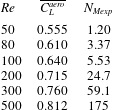
is the characteristic length equal to the square root of the wing area. The non-dimensional expected supportable total mass
 $N_{Mexp}$
for
 $L_{ref}=3.00$
mm for various values of the Reynolds number
 $Re$
is shown in table 4. The definition of
 $Re$
is the same as that in our previous study (Suzuki & Yoshino Reference Suzuki and Yoshino2018). By using these parameters, we calculate the values of the Reynolds number
 $Re$
and the wing-mass ratio
 $\text{W}\text{R}$
resulting in the upward flight and the downward flight when the characteristic length
 $L_{ref}=3.00$
mm as shown in figure 17. From this figure, we can find the same three regions (i)–(iii) as those observed in the simulations for the square wings (see figure 10). In these simulations, a large wing-mass ratio decreases aerodynamic force during translational motion in the same way as the simulations using the square wings, and these three regions are caused by the same mechanism as that for the square wings. Therefore, the effect of the wing mass on the translational motion is independent of the wing planform. Although we could not redo all the simulations and analysis by using the actual butterfly’s wings, it is expected that we can obtain the same conclusions as those obtained by using the square wings.
The time-averaged aerodynamic vertical force coefficient
 $\overline{C_{L}^{aero}}$
in the tenth stroke when the body of the model is fixed for an actual butterfly’s wings, and the non-dimensional expected supportable total mass
 $N_{Mexp}$
for
 $L_{ref}=3.00$
mm for various values of the Reynolds number
 $Re$
.

The values of the Reynolds number
 $Re$
and the wing-mass ratio
 $\text{W}\text{R}$
resulting in upward flight and downward flight when the characteristic length
 $L_{ref}=3.00$
mm for an actual butterfly’s wings.

As for simplification (2), Zheng, Hedrick & Mittal (Reference Zheng, Hedrick and Mittal2013) reported that the spanwise wing flexibility in the form of wing twist can improve the aerodynamic efficiency in the forward flight of butterflies. Due to the improvement in the aerodynamic performance by wing flexibility, the present results will be significantly changed when we incorporate flexibility into the wings of the model. We are now investigating the effects of the spanwise and chordwise wing flexibilities (Suzuki, Aoki & Yoshino Reference Suzuki, Aoki and Yoshino2019).
As for simplification (3), Liu, Dong & Li (Reference Liu, Dong and Li2016) reported that the body significantly enhances the vertical force in the forward flight of a cicada (Tibicen linnei). Although the width
 $w_{b}$
of the body is much smaller than the wing length for butterflies (
 $w_{b}\simeq 0.08L$
) unlike a cicada (
 $w_{b}\simeq 0.6L$
), the body might affect the aerodynamic performance in the forward flight of a butterfly as well. On the other hand, the body of the present model has a negligible effect since the width of the body is infinitely thin. The effect of the body on the aerodynamic performance in the forward flight of a butterfly requires further investigation.
In addition, it has been suggested by Dudley (Reference Dudley2002) and Suzuki et al. (Reference Suzuki, Minami and Inamuro2015) that the relative motion of the abdomen to the thorax might affect the attitude control of butterflies. This relative motion is neglected in the present model. The main issue of the present study is focused on the effect of wing mass on the aerodynamic performance, so attitude control is beyond the scope of the present study.
6.2 Limitation due to the wing kinematics of the model
The wing kinematics of the model (§ 2.2) are simplified in terms of the following points:
(4) The wing kinematics of the model are determined in a prescribed manner independently of the flight modes, e.g. take-off, climbing flight, forward flight and gliding flight, while actual butterflies might change the wing kinematics depending on the flight modes (Srygley & Thomas Reference Srygley and Thomas2002).
(5) The model changes the stroke plane by the attacking motion of the wings, while actual butterflies change it by the pitching motion of the body.
(6) The model does not change the lead-lag angle, while an actual butterfly changes it between approximately
$-10^{\circ }$
and
$10^{\circ }$
(Yokoyama et al.
Reference Yokoyama, Senda, Iima and Hirai2013).(7) The model changes the flapping angle between
$-45^{\circ }$
and
$45^{\circ }$
, while actual butterflies change it between approximately
$-33^{\circ }$
and
$69^{\circ }$
(Dudley Reference Dudley1990).(8) The model changes the attacking angle between
$0^{\circ }$
and
$90^{\circ }$
, while actual butterflies seem to change it effectively according to the flight mode since the attacking angle observed during take-off (Sunada et al.
Reference Sunada, Kawachi, Watanabe and Azuma1993b
) is different from that observed during forward flight (Yokoyama et al.
Reference Yokoyama, Senda, Iima and Hirai2013; Fei & Yang Reference Fei and Yang2015, Reference Fei and Yang2016).(9) The wing kinematics of the model are formulated by simple harmonic oscillations, while an actual butterfly’s wing kinematics are more complicated (e.g. Yokoyama et al. Reference Yokoyama, Senda, Iima and Hirai2013).
(10) The attacking motion of the wings and the pitching motion of the body are decoupled in the present model, while the geometrical AOA of an actual butterfly is determined as a result of the pitching motion of the body (Fei & Yang Reference Fei and Yang2015, Reference Fei and Yang2016).


The above simplifications (4)–(9) might suggest that the wing kinematics of the present model are artificial and far from those of actual butterflies. However, by comparing the present model with the more realistic model used by Fei & Yang (Reference Fei and Yang2016), we can see that the present model captures some features of the wing kinematics of actual butterflies. The butterfly model used by Fei & Yang (Reference Fei and Yang2016) was based on the experimental record of the flight motion of leaf butterflies, and the flapping angle and the AOA were approximated by simple harmonic functions without damaging the rough shapes of the curves of these angles. Although the definitions of these angles were different from those in the present study, we can rewrite these angles according to our definitions such as (2.8) and (2.9) as follows:
 $$\begin{eqnarray}\displaystyle & \displaystyle \unicode[STIX]{x1D703}(t)=\unicode[STIX]{x1D703}_{0}+\unicode[STIX]{x1D703}_{m}\cos \left(\frac{2\unicode[STIX]{x03C0}}{T}t\right), & \displaystyle\end{eqnarray}$$
 $$\begin{eqnarray}\displaystyle & \displaystyle \unicode[STIX]{x1D6FC}(t)=\unicode[STIX]{x1D6FC}_{0}+\frac{\unicode[STIX]{x1D6FC}_{m}}{2}\left[1+\cos \left(\frac{2\unicode[STIX]{x03C0}}{T}t+\unicode[STIX]{x1D6FE}\right)\right], & \displaystyle\end{eqnarray}$$
where
 $\unicode[STIX]{x1D703}_{0}$
is the centre of the flapping angle and
 $\unicode[STIX]{x1D6FC}_{0}$
is the minimum AOA. Fei & Yang (Reference Fei and Yang2016) set
 $\unicode[STIX]{x1D703}_{0}=32.5^{\circ }$
,
 $\unicode[STIX]{x1D703}_{m}=57.5^{\circ }$
,
 $\unicode[STIX]{x1D6FC}_{0}=43^{\circ }$
,
 $\unicode[STIX]{x1D6FC}_{m}=54^{\circ }$
and
 $\unicode[STIX]{x1D6FE}=\unicode[STIX]{x03C0}/2$
from the observation of leaf butterflies in forward flight. As for simplification (6) the lead-lag angle was not considered in their study. In addition to the wing kinematics, they used the wing shape captured by a leaf butterfly.
From the following three points, we can see that the present model captures some features of the wing kinematics of actual butterflies. First, by comparing (2.8) and (2.9) with (6.1) and (6.2), respectively, we can see that both wing kinematics have the same phase shift
 $\unicode[STIX]{x1D6FE}$
equal to
 $\unicode[STIX]{x03C0}/2$
. Due to this phase shift, the wings can be flapped downward and backward during downstroke and upstroke, respectively.
Second, we can see a common feature in the vortex structures released by the wings as shown in figure 18, which shows the vortices generated by the present model and those generated by the model that has a leaf butterfly’s wing shape and/or wing kinematics. Figure 18(a–c) is obtained by our simulations when the body of the model is fixed and
 $Re=500$
, whereas figure 18(d) was obtained by Fei & Yang (Reference Fei and Yang2016) when the butterfly model is in forward flight. From figure 18(a,b), we can see that DVs (vortices generated in the last downstroke) and UVs (vortices generated in the upstroke) are released downward and backward, respectively. From figure 18(a,c), we can see the same feature as that explained above, even when the wing shape is replaced by a leaf butterfly’s wing shape. The vortex structure shown in figure 18(a–c) can be seen in figure 18(d) as well. Especially, the vortex structures in figure 18(a,c,d) seem quite similar to each other.
Third, we can see a common feature in the time variations of the aerodynamic forces
 $C_{L}^{aero}$
and
 $C_{T}^{aero}$
as shown in figure 19, which shows the results obtained by our simulations when the body of the model is fixed and
 $Re=500$
. Unfortunately, the data obtained by Fei & Yang (Reference Fei and Yang2016) were not published in their paper. From this figure, we can see a common feature that a large positive peak in the vertical force appears in the downstroke, and that in the horizontal force appears in the upstroke. Due to these large positive peaks, the model can go upward and forward.
The vortex structures generated by (a) the present model with square wings and the present wing kinematics (2.8) and (2.9), (b) the model with square wings and a leaf butterfly’s wing kinematics (6.1) and (6.2), (c) the model with a leaf butterfly’s wing shape and wing kinematics and (d) the butterfly model used by Fei & Yang (Reference Fei and Yang2016), viewed from their right-hand sides. The results shown in (a–c) are obtained when the body of the model is fixed,
 $Re=500$
and the vortex structure is visualized by the isosurface of
 $Q=5(U_{tip}/L)^{2}$
at
 $t/T=10.23$
. The result shown in (d) is taken from Fei & Yang (Reference Fei and Yang2016). ‘DVs’ and ‘UVs’ refer to the vortices generated in the last downstroke and upstroke, respectively.

Time variations of (a) the aerodynamic vertical force coefficient
 $C_{L}^{aero}$
and (b) the aerodynamic horizontal force coefficient
 $C_{T}^{aero}$
for the present model with square wings and the present wing kinematics (2.8) and (2.9), for the model with square wings and a leaf butterfly’s wing kinematics (6.1) and (6.2) and for the model with a leaf butterfly’s wing shape and wing kinematics, when the body of the model is fixed and
 $Re=500$
.

In order to perform a more realistic simulation than the present simulation under simplification (4), one might consider that it is better to focus on one flight mode instead of the transitional motion from take-off to forward flight. For example, hovering and steady flapping flight have often been investigated for other insects in many studies (e.g. Aono, Liang & Liu Reference Aono, Liang and Liu2008; Liu Reference Liu2009; Liu et al. Reference Liu, Dong and Li2016), since these flight modes are regarded as fixed-point equilibriums where the body is at rest or moving at a constant speed due to the balance of gravitational force and torque, aerodynamic force and torque and inertial force and torque. To the best of our knowledge, however, such fixed-point equilibriums have not been observed in butterfly flights due to their body motion. Actually, Fei & Yang (Reference Fei and Yang2015) reported that using the assumption that a butterfly flies at a constant speed leads to either an underestimate of its speed or an overestimate of its generated lift due to the large time variation of flight speed, and consequently the fixed-point equilibrium at a constant speed is unrealistic in butterfly flights. Furthermore, it is difficult to numerically reproduce periodic equilibriums where the body motion changes periodically. Actually, Yokoyama et al. (Reference Yokoyama, Senda, Iima and Hirai2013) reported that even a realistic numerical model of a butterfly cannot achieve a periodic flight because the model cannot maintain the pitching angle in a proper range. This suggested that even a periodic flight mode cannot be found easily in butterfly flights. Therefore, it is difficult to assume the equilibriums not only at a constant speed but also with a periodic body motion. Although these reports are for actual butterflies, the same is equally true of the present model. The reason why we focus on take-off from the resting state and the transitional motion to forward flight is that these flight modes do not need to assume any kind of equilibrium.
As for simplification (10), the flapping aerodynamics and the attitude control cannot be decoupled associated with actual butterfly flight. The present model incorporates this simplification in order to avoid the difficulty of the attitude control. Without this simplification, we have to consider controlled flight where the pitching angle of the body is controlled and consequently the geometrical AOA is determined. It is quite difficult to achieve such controlled flights in numerical simulations, since the attitude control of butterflies has not been understood sufficiently. In addition, it is found in the present study that a large wing-mass ratio comparable to that of actual butterflies intensifies the time variation of the pitching angle (§ 5.1.3). This makes the simulations of the attitude control more difficult. In order to avoid the difficultly and to focus on the effect of wing mass on the aerodynamic performance, we use simplification (10) in the present study. The combination of the flapping aerodynamics and the attitude control will be investigated in future work.
6.3 Limitation due to the computational settings
The computational settings (§§ 3.2 and 4) are simplified in terms of the following points:
(11) The body motion of the model is limited to the translational motions in the
$x$
- and
$y$
-directions and pitching rotation, i.e. three degrees of freedom, while actual butterflies can perform translational motion in the
$z$
-direction and rolling and yawing rotation as well, i.e. six degrees of freedom (6DOF).(12) The wing–body motion of the model is assumed to be symmetric with respect to the longitudinal plane due to the mirror condition of the computational domain, while actual butterflies can perform asymmetric motions.


As for simplification (11), we could not find any simulation with 6DOF for butterflies, while there are a few simulations with 6DOF for other insects (e.g. Gao, Aono & Liu Reference Gao, Aono and Liu2011; Hino & Inamuro Reference Hino and Inamuro2018). This might be attributed to the erratic behaviour of butterflies. In addition, the longitudinal stability of butterflies has not yet been understood sufficiently. Simulations with 6DOF for butterflies are still challenging.
As for simplification (12), it was checked in the previous study by Suzuki et al. (Reference Suzuki, Minami and Inamuro2015) that the symmetry of the flow field with respect to the longitudinal plane is not broken at least until
 $Re=500$
when the motion of the model is limited in the longitudinal plane (simplification (11)). However, the symmetry might be broken when
 $Re>500$
, and consequently simplification (11) might become invalid. In addition, it was found in the previous study by Nakatani et al. (Reference Nakatani, Suzuki and Inamuro2016) that the same butterfly-like model as used in the present study cannot maintain the rolling angle in a proper range when the rolling motion of the model is considered and a small disturbance is initially added to the rolling motion. Therefore, in order to perform a more realistic simulation, it is necessary to investigate the motion with 6DOF.
As mentioned above, however, the longitudinal stability of butterflies has not yet been understood sufficiently. In addition, the pitching motion is one of the essential issues for arbitrary flapping air vehicles, since the instability in the pitching motion has been widely observed in flapping flight by insects independent of species (see Sun Reference Sun2014). Therefore, we focus on the effect of wing mass on the longitudinal motion of the butterfly-like model in this study. Simulations with 6DOF and attitude control for not only the pitching rotation but also the rolling and yawing rotations will be investigated in future work.
7 Conclusions
We have investigated the effect of wing mass on the free flight of a butterfly-like model by numerical simulations based on the IB-LBM. The model is composed of two square wings and a rod-shaped body, and the wings and the body are rigid and infinitely thin. The model flaps the wings downward to generate the lift force and backward to generate the thrust force like a butterfly. In the present study, we added the wing mass to the model and investigated its effect in terms of the wing-mass ratio
 $\text{W}\text{R}$
(the ratio of the wing mass to the total mass) and the wing-mass distribution
 $\unicode[STIX]{x1D70C}_{w}$
.
First, we investigated the effect of
 $\text{W}\text{R}$
when the mass is uniform over the wings. In the calculations of the inertial and aerodynamic forces and torques when the body of the model is fixed, we found that the magnitude of the inertial force is comparable to that of the aerodynamic force for
 $\text{W}\text{R}\geqslant 0.25$
, and the magnitude of the inertial torque is larger than that of the aerodynamic torque even for
 $\text{W}\text{R}\geqslant 0.1$
. From the simulations of free flight without rotation for various wing lengths
 $L=3.00$
–10.0 mm, various Reynolds numbers
 $100\leqslant Re\leqslant 900$
and various wing-mass ratios
 $0\leqslant \text{W}\text{R}\leqslant 1$
, we found that as
 $\text{W}\text{R}$
increases, the body tends to go up and down (back and forth) over a large distance due to the inertial force-induced vertical (horizontal) force during each stroke, and according to the body motion, the WTVs and the LEVs weaken and consequently the aerodynamic vertical and horizontal forces decrease. We defined the critical wing-mass ratio
 $\text{W}\text{R}_{c}$
between upward flight and downward flight and plotted it as a function of
 $Re$
. As a result, we found that the following three regions exist: (i)
 $\text{W}\text{R}_{c}=0$
, i.e. the model goes down even without wing mass, (ii)
 $\text{W}\text{R}_{c}$
steeply increases and (iii)
 $\text{W}\text{R}_{c}$
gradually decreases. In addition, we found that
 $\text{W}\text{R}_{c}$
can be expressed by a function of the non-dimensional total mass
 $N_{M}$
and is almost independent of the wing length
 $L$
. Therefore, we can predict the curve of
 $\text{W}\text{R}_{c}$
even for larger scales from the curves obtained by the present study. From the simulations of free flight with rotation, we found that the wing-mass ratio has a dominant effect on the rotational motion of the model, and a large wing-mass ratio reduces aerodynamic force and intensifies the time variation of the pitching angle.
Second, we investigated the effect of the wing-mass distribution
 $\unicode[STIX]{x1D70C}_{w}$
on the critical wing-mass ratio
 $\text{W}\text{R}_{c}$
as a function of
 $N_{M}$
. We considered the following five cases: the mass is uniform over the wings (Case 1); the mass is distributed linearly in the span direction, and the wing tip or the wing root is heavier (Cases 2-1, 2-2); the mass is distributed linearly in the chord direction, and the leading edge or the trailing edge is heavier (Cases 3-1, 3-2). Through simulations of free flight without rotation when
 $L=3.00$
mm and
 $Re=300$
, we found that the effect of the wing-mass distribution in the chordwise direction is less than that in the spanwise direction, and the range of the effect on
 $\text{W}\text{R}_{c}$
for all cases is confined to the range from
 $2/3$
to
 $4/3$
times as large as the
 $\text{W}\text{R}_{c}$
value for Case 1.
Finally, we discussed the limitations of the present model. Although the present model is highly idealized and simplified in many points, we found that the present model captures some features of actual butterflies. Therefore, the erratic behaviour of butterflies might be caused by their large wing-mass ratio.
Acknowledgements
This work was supported by JSPS KAKENHI grant number JP16K18012. The authors would like to thank Professor D. Asano at Shinshu University for guidance on scientific research writing in English. The authors would like to thank Professor T. Inamuro at Kyoto University for helping to enhance the readability of this paper. The authors would like to thank Mr F. Nakai for help with the formulation of the wing–body motion equations in appendix A.
Appendix A. Detailed form of equations of wing–body motion
In § 3.2, we expressed the wing–body motion by (3.8). The detailed forms of
 $\boldsymbol{{\mathcal{M}}}$
,
 $\boldsymbol{F}_{in}$
,
 $T_{in}$
and
 $T_{G}$
in this equation are given by
 $$\begin{eqnarray}\boldsymbol{{\mathcal{M}}}=\left[\begin{array}{@{}ccc@{}}{\mathcal{M}}_{11} & {\mathcal{M}}_{12} & {\mathcal{M}}_{13}\\ {\mathcal{M}}_{21} & {\mathcal{M}}_{22} & {\mathcal{M}}_{23}\\ {\mathcal{M}}_{31} & {\mathcal{M}}_{32} & {\mathcal{M}}_{33}\end{array}\right],\end{eqnarray}$$
where
 $$\begin{eqnarray}\displaystyle & {\mathcal{M}}_{11}={\mathcal{M}}_{22}=M, & \displaystyle\end{eqnarray}$$
 $$\begin{eqnarray}\displaystyle & {\mathcal{M}}_{12}={\mathcal{M}}_{21}=0, & \displaystyle\end{eqnarray}$$
 $$\begin{eqnarray}\displaystyle & {\mathcal{M}}_{13}={\mathcal{M}}_{31}=-m_{w}\{R_{\unicode[STIX]{x1D709}}\sin (\unicode[STIX]{x1D703}_{p}+\unicode[STIX]{x1D6FC})+R_{\unicode[STIX]{x1D702}}\cos (\unicode[STIX]{x1D703}_{p}+\unicode[STIX]{x1D6FC})\sin \unicode[STIX]{x1D703}\}, & \displaystyle\end{eqnarray}$$
 $$\begin{eqnarray}\displaystyle & {\mathcal{M}}_{23}={\mathcal{M}}_{32}=m_{w}\{R_{\unicode[STIX]{x1D709}}\cos (\unicode[STIX]{x1D703}_{p}+\unicode[STIX]{x1D6FC})-R_{\unicode[STIX]{x1D702}}\sin (\unicode[STIX]{x1D703}_{p}+\unicode[STIX]{x1D6FC})\sin \unicode[STIX]{x1D703}\}, & \displaystyle\end{eqnarray}$$
 $$\begin{eqnarray}\displaystyle & {\mathcal{M}}_{33}=I_{b}+m_{w}(\unicode[STIX]{x1D61A}_{\unicode[STIX]{x1D709}\unicode[STIX]{x1D709}}+\unicode[STIX]{x1D61A}_{\unicode[STIX]{x1D702}\unicode[STIX]{x1D702}}\sin ^{2}\unicode[STIX]{x1D703}), & \displaystyle\end{eqnarray}$$
and
 $$\begin{eqnarray}\displaystyle F_{inx} & = & \displaystyle m_{w}\left[R_{\unicode[STIX]{x1D709}}\{\ddot{\unicode[STIX]{x1D6FC}}\sin (\unicode[STIX]{x1D703}_{p}+\unicode[STIX]{x1D6FC})+(\dot{\unicode[STIX]{x1D703}}_{p}+\dot{\unicode[STIX]{x1D6FC}})^{2}\cos (\unicode[STIX]{x1D703}_{p}+\unicode[STIX]{x1D6FC})\}\right.\nonumber\\ \displaystyle & & \displaystyle +\,R_{\unicode[STIX]{x1D702}}\left\{\ddot{\unicode[STIX]{x1D6FC}}\cos (\unicode[STIX]{x1D703}_{p}+\unicode[STIX]{x1D6FC})\sin \unicode[STIX]{x1D703}+\ddot{\unicode[STIX]{x1D703}}\sin (\unicode[STIX]{x1D703}_{p}+\unicode[STIX]{x1D6FC})\cos \unicode[STIX]{x1D703}\right.\nonumber\\ \displaystyle & & \displaystyle \left.\!\left.+\,2\dot{\unicode[STIX]{x1D703}}(\dot{\unicode[STIX]{x1D703}}_{p}+\dot{\unicode[STIX]{x1D6FC}})\cos (\unicode[STIX]{x1D703}_{p}+\unicode[STIX]{x1D6FC})\cos \unicode[STIX]{x1D703}-(\dot{\unicode[STIX]{x1D703}}^{2}+(\dot{\unicode[STIX]{x1D703}}_{p}+\dot{\unicode[STIX]{x1D6FC}})^{2})\sin (\unicode[STIX]{x1D703}_{p}+\unicode[STIX]{x1D6FC})\sin \unicode[STIX]{x1D703}\right\}\right]\!,\qquad\end{eqnarray}$$
 $$\begin{eqnarray}\displaystyle F_{iny} & = & \displaystyle m_{w}\left[R_{\unicode[STIX]{x1D709}}\{-\ddot{\unicode[STIX]{x1D6FC}}\cos (\unicode[STIX]{x1D703}_{p}+\unicode[STIX]{x1D6FC})+(\dot{\unicode[STIX]{x1D703}}_{p}+\dot{\unicode[STIX]{x1D6FC}})^{2}\sin (\unicode[STIX]{x1D703}_{p}+\unicode[STIX]{x1D6FC})\}\right.\nonumber\\ \displaystyle & & \displaystyle +\,R_{\unicode[STIX]{x1D702}}\left\{\ddot{\unicode[STIX]{x1D6FC}}\sin (\unicode[STIX]{x1D703}_{p}+\unicode[STIX]{x1D6FC})\sin \unicode[STIX]{x1D703}-\ddot{\unicode[STIX]{x1D703}}\cos (\unicode[STIX]{x1D703}_{p}+\unicode[STIX]{x1D6FC})\cos \unicode[STIX]{x1D703}\right.\nonumber\\ \displaystyle & & \displaystyle \left.\!\left.+\,2\dot{\unicode[STIX]{x1D703}}(\dot{\unicode[STIX]{x1D703}}_{p}+\dot{\unicode[STIX]{x1D6FC}})\sin (\unicode[STIX]{x1D703}_{p}+\unicode[STIX]{x1D6FC})\cos \unicode[STIX]{x1D703}+(\dot{\unicode[STIX]{x1D703}}^{2}+(\dot{\unicode[STIX]{x1D703}}_{p}+\dot{\unicode[STIX]{x1D6FC}})^{2})\cos (\unicode[STIX]{x1D703}_{p}+\unicode[STIX]{x1D6FC})\sin \unicode[STIX]{x1D703}\right\}\right]\!,\qquad\end{eqnarray}$$
 $$\begin{eqnarray}\displaystyle & T_{in}=-m_{w}\left[\unicode[STIX]{x1D61A}_{\unicode[STIX]{x1D709}\unicode[STIX]{x1D709}}\ddot{\unicode[STIX]{x1D6FC}}+\unicode[STIX]{x1D61A}_{\unicode[STIX]{x1D709}\unicode[STIX]{x1D702}}(\ddot{\unicode[STIX]{x1D703}}\cos \unicode[STIX]{x1D703}-\dot{\unicode[STIX]{x1D703}}^{2}\sin \unicode[STIX]{x1D703})+\unicode[STIX]{x1D61A}_{\unicode[STIX]{x1D702}\unicode[STIX]{x1D702}}\{\ddot{\unicode[STIX]{x1D6FC}}\sin ^{2}\unicode[STIX]{x1D703}+2\dot{\unicode[STIX]{x1D703}}(\dot{\unicode[STIX]{x1D703}}_{p}+\dot{\unicode[STIX]{x1D6FC}})\sin \unicode[STIX]{x1D703}\cos \unicode[STIX]{x1D703}\}\right]\!, & \displaystyle \nonumber\\ \displaystyle & & \displaystyle\end{eqnarray}$$
 $$\begin{eqnarray}\displaystyle & T_{G}=m_{w}G\{-R_{\unicode[STIX]{x1D709}}\cos (\unicode[STIX]{x1D703}_{p}+\unicode[STIX]{x1D6FC})+R_{\unicode[STIX]{x1D702}}\sin (\unicode[STIX]{x1D703}_{p}+\unicode[STIX]{x1D6FC})\sin \unicode[STIX]{x1D703}\}. & \displaystyle\end{eqnarray}$$
Appendix B. Convergence study
In order to check whether the present results are sufficiently resolved, we perform the free-flight simulations without rotation for various spatial resolutions when
 $L=3.00$
mm,
 $Re=300$
and
 $\text{W}\text{R}=0.1$
.
At first, in the same way as § 5.1.2, we calculate the non-dimensional expected supportable mass when the body of the model is fixed. Table 5 shows the spatial and temporal resolutions for the convergence study, and the results of the time-averaged aerodynamic vertical force coefficient
 $\overline{C_{L}^{aero}}$
and the non-dimensional expected supportable total mass
 $N_{Mexp}$
. We can see from this table that the deviation of
 $N_{Mexp}$
between the results when
 $L\geqslant 50\unicode[STIX]{x0394}x$
and
 $L=80\unicode[STIX]{x0394}x$
is within 4 % at most.
Spatial and temporal resolutions for the convergence study when
 $L=3.00$
mm,
 $Re=300$
and
 $\text{W}\text{R}=0.1$
. The wing length
 $L$
and the flapping period
 $T$
are multiples of the lattice spacing
 $\unicode[STIX]{x0394}x$
and the time step
 $\unicode[STIX]{x0394}t$
, respectively. The time-averaged aerodynamic vertical force coefficient
 $\overline{C_{L}^{aero}}$
is calculated in the tenth period (
 $9.0\leqslant t/T\leqslant 10.0$
), and the non-dimensional expected supportable total mass
 $N_{Mexp}$
is calculated by (5.4).

Next, we calculate the free flight without rotation when the non-dimensional total mass is equal to the above results for various spatial resolutions. Figure 20 shows the trajectories of the centre of the body for various spatial resolutions. We find that the results when
 $L\geqslant 50\unicode[STIX]{x0394}x$
are reasonably comparable with those when
 $L=80\unicode[STIX]{x0394}x$
. According to these results, we use the resolution shown in table 1.
The trajectories of the centre of the body for various spatial resolutions when
 $L=3.00$
mm,
 $Re=300$
and
 $\text{W}\text{R}=0.1$
.

Appendix C. Effect of the definition of upward/downward flight
In order to check the effect of the definition of upward/downward flight shown in § 5.1.3, we compare the three results when the integration interval
 $[t_{1},t_{2}]$
of the time-averaged vertical velocity
 $V_{m}$
in (5.6) is
 $[0,20T]$
,
 $[10T,20T]$
and
 $[15T,20T]$
. Figure 21 shows the results for
 $L=3.00$
mm. Figure 21(a) is the same as figure 10, although the curve of the critical wing-mass ratio and some plots are omitted. In figure 21(a–c), we can find the same three regions (i)–(iii) as those shown in figure 10. In addition, we find that the quantitative difference between figure 21(a–c) is not significant. Therefore, we can conclude that the discussion in § 5.1.3 is not affected by the choice of the integration interval of
 $V_{m}$
.
The values of the Reynolds number
 $Re$
and the wing-mass ratio
 $\text{W}\text{R}$
resulting in upward flight and downward flight for
 $L=3.00$
mm when the integration interval in the time-averaged vertical velocity
 $V_{m}$
is (a)
 $[0,20T]$
, (b)
 $[10T,20T]$
and (c)
 $[15T,20T]$
.