


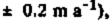
 is nearly half of the total excess outflow for the Ice Stream Β system (20 ± 4 km


 .


Introduction
Recent mass-balance studies of the “Ross” ice streams (ice streams A-F), which discharge 95% of the total ice drained from the West Antarctic ice sheet into Ross Ice Shelf, suggest an overall negative net-balance rate for the ice streams and their catchment area (Reference Shabtaie and BentleyShabtaie and Bentley 1987). This was originally suggested by Reference HughesHughes (1975), although Reference RoseRose (1979) and Reference Thomas, MacAyeal, Eilers, Gaylord, Bentley and HayesThomas and others (1984) concluded that the ice-stream discharges were in balance with the ice accumulated on the ice streams and in their catchment area. Reference Shabtaie and BentleyShabtaie and Bentley (1987), using new ice-stream boundaries and the grounding lines obtained by radar sounding (Fig. 1), calculated the output fluxes for all the ice streams, ridges, and domes draining into Ross Ice Shelf at gates close to the new grounding lines. The input flux for each individual catchment area was calculated also from the available measurements of snow-accumulation rates. These measurements showed the output flux for Ice Stream Β to be twice the input flux, and also indicated a negative net balance for Ice Stream A. Reference Whillans, Bolzan and ShabtaieWhillans and others (1987) also show a strongly negative mass balance for Ice Stream B. On the other hand, Ice Stream C, which is now stagnant, showed a negligible output flux, 37 times lower than the input flux. The mass-balance calculation for ice streams Β and C (Reference Shabtaie and BentleyShabtaie and Bentley 1987) showed that the combined mass input of these two ice streams is nearly equal to their combined mass output at the grounding line. This has re-emphasized the question whether in this West Antarctic system one fast-mode ice stream could grow at the expense of another and capture its catchment area, as suggested by Reference RoseRose (1979). In this study, the mass-balance calculations for ice streams A and Β have been extended up-stream by considering the fluxes through several gates across the ice streams at locations where velocities and ice thicknesses were measured. Furthermore, we have calculated fluxes separately for ice streams Bl and B2 (the two branches of Ice Stream B). In addition, we use recently presented surface-elevation data (Fig. 2, from Reference Shabtaie, Whillans and BentleyShabtaie and others (1987)) to shed further light on the ice-stream-capture hypothesis.
Map of the West Antarctic ice streams A, B, and C, and their associated flow bands on Ross Ice Shelf. 1984–85 radar flight lines (solid) and selected RIGGS (1973–78) flight lines (dotted) are shown. The heavy shading is the marginal shear zone (active or relict) of the ice streams. The light shading is the relatively less chaotic part of the ice streams and their flow bands. The dashed lines in Ice Stream A and in the grid north-western corner of the ice shelf are flow lines; the dashed lines between ice streams Β1 and B2 mark the central suture zone. The margins that are not solely based on surface clutter between ice-stream flow bands on the ice shelf are shown by long-dashed lines. The base camps (UB, DB, UC, DC, and CR) are shown by triangles. The ice rises are shown by a solid line and no shading inside. The dots are University of Wisconsin stations, circles are Ohio State University and OSU-NASA co-operative stations (Reference Whillans, Bolzan and ShabtaieWhillans and others 1987), and squares are University of Chicago-NASA stations (Reference Bindschadler, Stephenson, MacAyeal and ShabtaieBindschadler and others 1987). The origin of the rectangular grid coordinate system used on this and succeeding maps is at the South Pole; grid north is toward Greenwich and therefore toward the top of the map. Squares are 1° of latitude on a side.

Mass Conservation of the Ice Stream
The boundaries of the ice streams are marked by marginal shear zones that consist of many crevasses in a chaotic, incoherent pattern. These disturbed zones produce back-scattered radar echoes (clutter) that are easily identified on the radar records, thus providing an excellent means of mapping the boundaries of the ice streams. In order to calculate the mass balance along the ice streams, flow bands were constructed, using the lateral boundaries obtained by radar sounding and a series of transverse gates (Fig. 3). All but one of the gates were chosen to coincide with radar flight lines, which provide accurate determinations of ice thicknesses and the positions of the ice-stream margins at the ends of each gate. The exception is gate GO, which was constructed at the head of Ice Stream Β by using the margins of ice streams Bl and B2 (extrapolated in the case of B2), the surface-elevation map, and velocity vectors from Reference Whillans, Bolzan and ShabtaieWhillans and others (1987). In our co-ordinated work, the radar flights passed over several ground-control stations where velocities were measured by doppler satellite-tracking techniques (Reference Bindschadler, Stephenson, MacAyeal and ShabtaieBindschadler and others 1987, Reference Shabtaie and BentleyShabtaie and Bentley 1987,Reference Whillans, Bolzan and Shabtaie Whillans and others 1987).
If we assume a constant mean density, the conservation of mass within each flow band can be expressed in terms of volume fluxes (Fig. 4a):
Map of (he ice streams and their catchment boundaries, ice rises, and grounding zones in the Siple Coast region, together with surface-elevation contours (solid lines). Contour intervals are 10 m up to 120 m (the 110 m contour line over Crary Ice Rise is omitted), 20 m from 120 to 200 m, 40 m from 200 to 1000 m, and 100 m at higher elevations. The depiction of ice streams, ice rises, and their boundaries, is the same as in Figure 1. 1984–85 stations (dots), RIGGS stations (open circles), IGY Ross Ice Shelf surface-traverse stations (open squares), and IGY oversnow-traverse stations (small dots) are shown. Grounding lines and ice-rise boundaries are shown by short-dashed lines. The long-dashed lines are the boundaries between the two confluent ice streams Bl and B2, and ice streams Bl and A. The long-dashed dotted lines are the boundaries of the drainage systems A, B, and C. The hachured zone around and up-stream of Crary Ice Rise is intensively crevassed and locally grounded (ice rumples). In this zone the ice is moving an order of magnitude faster than Crary Ice Rise or the four ice rises flanking Crary Ice Rise.

Map showing the positions of the gates across the ice streams (heavy lines), through which the fluxes are calculated (inTable I andII ). Velocity and ice-thickness profiles are shown in Figures 5, 6, 7, and 8. The depiction of ice-streams, grounding lines, ice rises, their boundaries, and ground-control stations is the same as in Figure 2. The designations of some of the ground-control stations (i.e. 51, A19, etc.) are shown. The dashed-dotted lines are the drainage-system boundaries and are the same as in Figure 2.


where F i is the flux through the input gate, F r and F l are fluxes entering from the sides, F s (the flux at the upper surface) is the product of the surface area (S) and the mean snow accumulation rate

Fb (the flux at the bottom surface) is the product of S and the mean bottom melt rate

F out is the flux through the output gate, and F net is the rate of volume change within the band. The flux through a gate is given simply by

where H is the ice thickness, v is the column-mean velocity across the appropriate gate, and y is the transverse coordinate (normal to velocity vectors and the_marginal shear zone). For our calculations we replace v by the surface velocity; this should introduce a negligible error not only because basal sliding is dominant, but also because we are calculating differences between inflow and outflow.
The ice thicknesses and velocities along the margins of the ice streams are not as well known as those along the gates, because there were no continuous flight lines along them. Therefore the lateral flux along each margin was calculated by means of the product of marginal velocities and ice thicknesses where they were measured at the ends of the gates.
Snow-accumulation rates for the calculation of F s were taken from a map compiled by Shabtaie and Bentley (1987) from several data sources. The basal flux (Fb) is unknown, but is surely negative (melting) beneath an active ice stream. Estimates of basal melt rates under ice streams range from a few millimeters (Reference Budd, Jenssen and RadokBudd and others 1971) to several centimeters (Reference RoseRose 1979). At the base of the floating ice shelf, melting and freezing are both possible. Reference Zotikov, Zagorodnov and RaikovskyZotikov and others (1980) report 6 m of saline ice at the bottom of a core taken from the Ross Ice Shelf Project (RISP) drill site (J9) in the B2 flow band; based on a newly determined position of the grounding line up-stream, Shabtaie and Bentley (1987) calculated a mean bottom-freeze

aincludes the bottom melt/freeze term
bincludes half of the output flux from ridge AB
rate of about 12 mm a−1. On the other hand, thermodynamic calculations by Reference MacAyealMacAyeal (1984) indicate that melting should occur within the area in question. Since the melt/freeze rate at specific points is unknown and cannot be estimated independently, all we really can calculate is F net + F b. Thus, defining F in = F i + F l + F r + F s,

We can also present the results in terms of equivalent mean thickening

plus mean bottom-melt

rates:

Although F b is not known, beneath the ice streams it is surely small compared to the uncertainty in measuring F net. The uncertainty in

is several tens of centimeters, at least an order of magnitude greater than

On the ice shelf, however,

could be significant. Then, in Table I,

and the tabulated thickening or thinning rate,

, is the actual thinning rate only if F b = 0. Although it is important to have the estimate of the melt/freeze rate, it is not necessary for our general conclusions, because it is certainly much smaller than most of the values of

calculated for the flow bands (Table I).
The boundaries and configuration of all the flow bands were defined solely from the radar sounding. No velocity or strain data were used in their construction. This has the advantage that the boundaries are directly observed at each crossing, so position error does not accumulate along the flow line, as it does when tracing a flow line by interpolating between velocity measurements. On the other hand, we must recognize that if the boundaries of an ice stream have shifted with time, the radar tracks (which represent markers that have been inserted into the ice at some past time, e.g. when the ice first entered the ice stream and was crevassed) are not necessarily everywhere parallel to the present-day stream lines.
Analysis
Errors were assigned as follows. The measurement error in determining ice thickness by radar sounding is ±1%, stemming principally from a 1% uncertainty in the wave speed, which was taken to be 171 m (μs)−1 (the 0.05 μs uncertainty in travel time is a minor contributor). There were a few cases where part of the bottom echoes were questionable, because they were obliterated by the clutter generated from a shear margin. In that case the thicknesses were interpolated or, in two cases, part of the ice-thickness profile was estimated from Reference RoseRose (1979). For interpolated thicknesses the error is proportional to the local ice-thickness gradient; in the worst case (a gradient of 10−1 rad) the error in average ice thickness across that section is 10%. All the ice thicknesses were reduced to solid-ice equivalents by subtracting the firn correction height of 17 m (Shabtaie and Bentley 1982).
The surface velocities were determined by repeat positioning from Transit satellites, using Magnavox MX1502 and JMR-1 receivers. The point-position method for about 30 passes will result in velocity errors of about 10 m a−1 (most of the stations were occupied for more than 1 d; thus more than 30 passes were recorded). More accurate velocities are obtained by the translocation method using two fixed stations, which yields errors less than about 3 m a−1 (Reference Whillans, Bolzan and ShabtaieWhillans and others 1987). The velocity is assumed to vary smoothly between stations at which measurements were made.
The velocities across Ice Stream Β gate G5 (Figs 3 and 6b) are known essentially continuously because of the density of the stations and because optical measurements were made between the satellite stations. Furthermore, the velocities in the grid south-western marginal shear zone of this gate were measured by optical resectioning of the seracs within the shear margin from a stationary station on ridge BC (Reference Bindschadler, Stephenson, MacAyeal and ShabtaieBindschadler and others 1987). The measurements on gate G5 show a velocity variation of about 6% across most of the ice stream. The transverse velocities measured by Reference Whillans, Bolzan and ShabtaieWhillans and others (1987) around the Upstream Β camp (UB) show a velocity variation within the ice stream of about 1%. There are two stations (11 and 22 in Fig. 3) that are located near the inner boundaries of the marginal shear zones of ice streams Bl and B2 — the velocities there are also nearly the same as those at neighboring stations located more centrally in the ice streams. We thus assume a slight drop (in accordance with velocities along G5) near the inner edge of the marginal shear zone on each gate.
Within the shear margin of gate G5, the velocities drop linearly to the low value characteristic of ridge BC. Thus, for all the other gates, the velocities were also taken to vary linearly across the marginal shear zones. The widths of the shear margins are not constant along the ice streams; they vary by a factor of 2 or 3, which modifies the velocity profile.
We assume that there is no shear zone between ice streams Bl and B2 down-stream of their junction, since the stations on each side of the suture zone do not show noticeably different velocities. However, the velocity across gate G5 does show a 5% decrease at the suture zone. We do not know whether this velocity pattern continues up-stream — it may instead reflect the presence downstream of the clutter-free feature known as “ice rise a”, even though “ice rise a” is known to be moving now at about the same velocity (460 m a−1) as the neighboring ice (Reference Bindschadler, Stephenson, MacAyeal and ShabtaieBindschadler and others 1987). If “ice rise a” was stationary not long ago, and has recently become unpinned, it could formerly have exerted back pressures up-stream that slowed the velocities there. If it has recently become “unpinned”, velocities up-stream may not yet have adjusted fully.
Based on the velocity variations on gate G5, and at UB, the error on the velocity profile is taken to be 5%.
The effect of navigational errors on the width of each gate is small. The total misclosure in a flight totalling 1000 km averages less than 3 km. If ties were made to field stations of known position along the route, as was usually the case, the misclosure was diminished. Nevertheless, in order to be conservative, and to include plotting error, we will adopt a distance error of ±1%.
Heading errors also must be considered. Flights across the flow bands are nearly parallel to the ice-thickness contours. Therefore an undetected lateral displacement of the flight line will introduce a thickness error that is proportional to the product of that displacement and the ice-thickness gradient. The steepest gradients on the ice stream are about 5 × 10⁻³, so a 1 km displacement (1% of a 100 km wide gate) yields an error in ice thickness of ±50 m for that segment of the gate (this value is an order of magnitude lower for the gates close to the grounding lines).
Finally, there is an error in width of the flow band that results from the fact that the flights are not exactly normal to the stream lines (this is the case for gates G8 and G9 of Ice Stream A; all the other gates are very close to flight lines) — stream lines must therefore be extrapolated from the flight lines to the lines of the gates. We estimate this error at ±2%.
The errors in the fluxes from sides of the flow bands (F r and F e) are up to 50% of the input flux because of the small magnitude of the velocities and the poor sampling. Nevertheless, these errors are not important, as both the lateral fluxes and their errors are an order of magnitude smaller than the fluxes through the end gates.
The fluxes from snow accumulation (F s) are also comparatively small, so the errors in accumulation rates are also negligible.
Results
The velocities and thicknesses through all the gates are shown in Figures 5–8, and the calculated fluxes are given in Table I. The fluxes for ice streams Bl and B2 are listed separately, together with the totals for Ice Stream B. Net fluxes range between −8 and +6 km3 a−1; several are significantly different from zero.
Fig. 4. (a) Idealized diagram of one block of an ice-stream flow band, showing the fluxes entering and exiting the band. These fluxes are defined by (Equationequ.1) and (equ.2), and their values are listed in Table I andTable II. (b) Sketch map of sections of the ice stream that show unsteady transient and expansion behavior. The arrow at the center of the block shows the flow direction; the input (W i) and output (W o) gates are shown. The relict boundaries of stagnant ice rises and shear margins are shown by dashed lines; the chaotic pattern shows the present shear margins. See the text for a detailed explanation of each case.


Velocity profiles (solid line; the scale is shown on the left-hand side) and ice-thickness profiles (dashed line; the scale is shown on the right-hand side) versus distance, across the flow-band gate G0, of Ice Stream Β and parts of ridges AB and BC (Fig. 3). The heavy shadings are the marginal shear zones.

Fig. 6. Velocity profiles (solid line; the scale is shown on the left-hand side) and ice-thickness profiles (dashed line; the scale is shown on the right-hand side) versus distance, across the flow-band gates Gl, G2, G3, G4, G5, and G6 of Ice Stream Β (Fig. 3). The heavy shadings are the marginal shear zones.

Fig. 7. Velocity profiles (solid line; the scale is shown on the left-hand side) and ice-thickness profiles (dashed line; the scale is shown on the right-hand side) versus distance, across the flow-band gates G11 of Ice Stream A, G7 of Ice Stream B, and G13 of Ice Stream C. These gates are located down-stream of Crary Ice Rise (Fig. 3).

Fig. 8. Velocity profiles (solid line; the scale is shown on the left-hand side) and ice-thickness profiles (dashed line; the scale is shown on the right-hand side) versus distance, across the flow-band gates G8, G9, and G10 of Ice Stream A (Fig. 3). The heavy shadings are the marginal shear zones.

In contrast to the case for rock-confined outlet glaciers, changes in net flux on an ice stream within a block may be a transient effect arising from changes in the ice-stream boundaries. If, for example, a piece of an adjoining ridge that demarcates an ice stream has recently been incorporated into the ice stream, i.e. if the ice stream has expanded in width, and if insufficient time has passed for a new equilibrium velocity to be established, then the flux through a gate at that point will have increased. On an ice stream otherwise in balance this will result in a nel flux that is positive down-stream and negative up-stream.
This point is illustrated in Figure 4b. Six cases of ice-stream expansion are illustrated, in which an idealized flow-band block of an ice stream has incorporated a mass of formerly slowing moving ice into its area. That added mass may come from the bordering ridge (cases I, III, V, and VI), by activation of a formerly stationary “island” within the ice stream (cases II and VI), or from the tip of a “peninsula” at the junction of two ice-stream branches (case II). In cases I and II an increase in width (ΔW o) of the ice stream will add a transient flux at the output gate, so that the net flux of a block otherwise in balance will be negative. The associated thinning within this block, at least at first, will be concentrated in some way in and around the added mass. In cases 111 and IV there is an opposite effect. Since the added mass is within the input gate, the net flux of a block otherwise in balance will be positive and there will be transient, initially localized, thickening within the block. In case V the whole margin has migrated toward the neighboring ridge; this can be thought of as a combination of cases I and II, so the net result depends upon the difference between the added fluxes at the two ends. Finally, case VI portrays two cases of changes entirely within a flow-band block; no change will be measured until a mass passes through the output gate.
Just what the time constant is for transient decay is difficult to say. We estimate that it will be of the order of 100 years, based on the study by Reference Alley, Blankenship, Rooney and BentleyAlley and others (1987) of the propagation of transient disturbances up and down a model ice stream. If that is correct, then the transient net fluxes will persist for some decades after the incorporation of the added masses into the ice stream.
Ice Stream Β
The output fluxes for block G0-G1 (i.e. the section of the flow band between gates GO and GÌ) are significantly higher than the input fluxes; Ice Stream ΒI has a larger imbalance than Ice Stream B2. The equivalent thinning rate for Ice Stream Bl is 1.3 m a−1, about twice that for Ice Stream B2. We interpret this negative net flux, combined with the positive net flux in the adjacent down-stream block (GI-G2), as indicating some combination of headward growth and expansion of the ice streams at the expense of both the radar-clutter-free “island zone” between them and ridges AB and BC. This interpretation is strongly influenced by the radar and ice-velocity data, which suggest piecemeal break-up of the regions surrounding the ice stream in this block, and the incorporation of “rafts” into the ice stream (Reference Shabtaie, Whillans and BentleyShabtaie and others 1987, Reference Whillans, Bolzan and ShabtaieWhillans and others 1987).
The net flux for block G1-G2 is positive; Ice Stream B2 shows a thickening rate that is more than twice that for Ice Stream Bl. We believe that this thickening reflects the incorporation of “island-zone” ice into ice streams Bl and B2, with the rate of incorporation decreasing down-stream, or that it is caused by intense thinning in the up-stream area (block G0-G1). We note, however, that Reference Whillans, Bolzan and ShabtaieWhillans and others (1987), citing their results as preliminary, did not find a significant imbalance for a “small-area” calculation within this flow band.
Gate G3 is located where Ice Stream Β narrows and the two branches converge. The net flux in block G2-G3 is not significantly different from zero. The same is true for block G3-G4, although there is a suggestion of a shift in flux from Ice Stream Bl to Ice Stream B2. (Whillans and others (1987) found strong “small-area” imbalances in Ice Stream Bl within blocks G2-G3 and G3-G4, but none within Ice Stream B2.) This apparent shift is even stronger in block G4—G5, in which the net flux for Ice Stream Bl is strongly positive and that for Ice Stream B2 is strongly negative, whereas the block as a whole is in balance. The shift is also apparent in the widths of the gates — gates G4 and G5 for Ice Stream Bl are about the same width, whereas in the case of Ice Stream B2, gate G5 is twice as wide as gate G4. The shifting geometry, together with the overall zero net flux for the block, suggests to us that the suture zone may not be a flow line in this sector (which is what we had assumed in this calculation) — ice may flow across it from Ice Stream Bl into Ice Stream B2; however, measured velocities at gate G2 do not show such a shift taking place (Reference Bindschadler, Stephenson, MacAyeal and ShabtaieBindschadler and others 1987). Such a shift might mean that there was a lateral shift in the position of the point of confluence up-stream some 200–300 years ago, when the ice now in block G4-G5 was at that point. (For a similar interpretation of Ross Ice Shelf down-stream of Crary Ice Rise, see Reference JezekJezek (1984).) Alternatively, Ice Stream B2 might be growing laterally into ridge BC around gate G5 (or shrinking around gate G4); in this case, the fact that the net fluxes for the two ice streams are so nearly equal and opposite would be simply a coincidence.
Whatever the reason, there is a definite flux shift from Ice Stream ΒI to Ice Stream B2 between gates G4 and G5. Down-stream, since Ice Stream B2 is much broader than Ice Stream Bl, it receives more mass input at the surface, so its flux excess over Ice Stream Bl continues to grow. The net result is that, whereas at their heads ice streams Bl and B2 carry about the same flux, through gate G7 Ice Stream B2 discharges more than twice as much as Ice Stream Bl.
Within block G5-G6 there is a suggestion of a negative net flux, although it is not significant at the 2 σ level. This is a weakly grounded area (i.e. an area whose surface is only slightly higher than it would be if the ice were afloat) whose ice-shelf-like surface slope (0.35 × 10⁻³) is an order of magnitude lower than that of the main body of the ice stream (Fig. 2). Within this block there is at least one ice-rise-like feature, formerly called “ice rise a” (the existence of “ice rise A” is questionable) (Fig. 3). This feature is not really an ice rise at all now, because it is moving with the same speed (465 m a−1) as surrounding ice (Reference Bindschadler, Stephenson, MacAyeal and ShabtaieBindschadler and others, 1987) — it is now called “ice raft a”. However, its crevasse-free surface (i.e. absence of radar clutter) and buried boundary crevasses (also seen by radar) suggest that it once was a true, stationary ice rise. If some ice within block G5-G6 has recently become unpinned, as this interpretation would imply, and if some “activated” ice is now passing through gate G6, then the higher output flux would tend to cause a negative net flux. Perhaps “ice raft a” (and “ice rise A”, if it exists) were once part of a much more extensive Crary Ice Rise. Another possible contributor to a negative net flux is the lateral expansion of the ice stream with time, that expansion being progressively larger down-stream. Such a model might explain the broadening of Ice Stream Β in this block.
The last gate (G7) was constructed on the ice shelf down-stream of Crary Ice Rise. The net flux for block G6—G7 is not significantly different from zero, although there is a suggestion of a positive imbalance in the ΒI part. MacAyeal and others (in press) calculate a thickening plus melt rate of about 0.1 ± 0.1 m a−1 for an area flanking the Crary Ice Rise complex. The small indicated value for

(really H plus the bottom melt rate

on the ice shelf) in flow band B2, i.e. less than about 0.2 m a−1, is consistent with other evidence. Some bottom freezing is reported for this area (Reference Zotikov, Zagorodnov and RaikovskyZotikov and others 1980), but at a mean rate of only about a centimeter per year (Shabtaie and Bentley 1987). For a flow band located within the G6-G7 (B2) flow band, Reference Thomas and BentleyThomas and Bentley (1978) calculated a value for

that was not significantly different from zero, with a standard error of 70 mm.
Ice Stream A
Four gates have been chosen for Ice Stream A; two are located in the main part of the ice stream, a third is at the grounding line (Fig. 8), and the fourth, a continuation of G7 on Ice Stream B, is 270 km down-stream of the grounding line (Fig. 7). There is no net flux in any of the blocks that is significantly different from zero at the 2 σ level. Nearly equal and opposite net fluxes in blocks G8-G9 and G9-G10 suggest a slight overestimation of the flux through gate G9, for which there is only one velocity measurement. However, the combined fluxes (5.7 ± 3.0 km3 a−1) in the two ice-shelf blocks (G6-G7 (B2), and G10-G11 (A)) grid north of Crary Ice Rise do suggest an

of 0.26 ± 0.13 m a−1 in the channel between Crary Ice Rise and the Transantarctic Mountains.
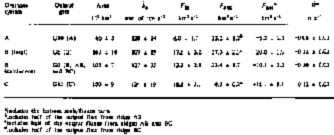
aincludes the bottom melt/freeze term
bincludcs half of the output flux from ridge AB
cincludes half of the output fluxes from ridges AB and BC
dincludes half of the output flux from ridge BC
Ice Stream C
At present, system C as a whole is thickening

. As yet, we have insufficient information to say how

may vary from place to place. For example, it is conceivable that

on the surface ridge that lies along grid 4°W, as ice flows both grid westward into the neighboring depression, and grid eastward down the main slope. Many more velocity measurements will be needed to define what may be a complex velocity field.
Mass balance of the ice-stream drainage system
Shabtaie and Bentley (1987) compared the volume outflow of the ice streams with their accumulated ice volume in their catchment areas. The net fluxes for ice streams A and Β are negative (Table II); that for Ice Stream C is strongly positive. The 37: 1 ratio of input to output for the Ice Stream C system is a direct result of the stagnancy of Ice Stream C itself. Neighboring system B, on the other hand, shows a 2 : 1 ratio of output to input. This large imbalance has led us to calculate the fluxes at the head of Ice Stream Β and up-stream of it. The total flux through gate G0 (AB, Β, and BC) (Figs 3 and 5) is the sum of the fluxes for the main part of Ice Stream Β (18.8 ± 1.4 km3 a−1; Table I) and the contributions from ridges AB (4.5 ± 0.9 km3 a−1) and BC (0.2 ± 0.02 km3 a−1; not tabulated): 23.4 ± 1.7 km3 a−1. The input to the catchment area up-stream of this gate is only 13.3 ± 2.8 km3 a−1 (Table II), so net flux for the catchment part of system Β is −10 ± 3 km3 a−1. As the net flux for the whole system Β (with the output at gate G6 (B)) is −20 ± 4 km3 a−1, about one-half of the imbalance between input and output fluxes occurs on the body of the ice stream, and about half in the catchment area. This suggests not only that Ice Stream Β is expanding between gates GO and G6, but that the disturbance is propagating up-stream into the catchment area. At present, it is not clear how far this disturbance has traveled up into the catchment, since velocities are not known up-stream of Gate GO. However, the surface-elevation contours (Fig. 2) suggest that the grid southern boundary of system Β grid west of grid 5°W is moving (or has moved) laterally toward Ice Stream C, causing a marked asymmetry to ridge BC.
Ridges AB and BC
The mean slope of ridge AB (Fig. 2) indicates that there is flow from the main inland ice sheet into this region. The velocity at station 60 near the margin of Ice Stream Bl (Fig. 3) is high — 74 m a−1 to the grid south; even near the axis of the ridge at station SC (Fig. 3) it is 17 m a−1 (Whillans and others 1987), which is too high to be balanced by local snow-fall on the ridge. We estimate the input flux at gate GO (AB) to be 4.5 ± 0.9 km3 a−1 (there could be a substantial error in the velocity profile) (Fig. 5); the velocity at the grid eastern end was assumed to be the same as at station SC, and the interpolated shape of the velocity profile was simply taken to be linear. If we add to that, the flux through the system A part of ridge AB (2.6 ± 0.5 km3 a−1), we find a total flow from the main inland ice sheet into ridge AB of about 7.1 ± 1 km3/year. This almost equals the flux through gate G0 into Ice Stream Bl. From the convoluted surface-elevation contours, ridge AB appears to be much more active than Siple Dome or the down-stream end of ridge BC.
Since the velocities from ridge AB into Ice Stream A are largely unknown, we will consider the flux balance only for the system Β part of ridge AB. The output flux into Ross Ice Shelf is 1.2 ± 0.4 km3 a−1; we assume half of that to be part of system B. Our estimates of the fluxes into Ice Stream Bl are shown in the F l + F r column for Ice Stream Bl (Table II); the total is 5.9 ± 0.7 km3 a−1. The input flux from snow accumulation over this area is 1.0 ± 0.2 km3 a−1. Therefore the total input- and output-flux estimates for the system Β part of ridge AB are 5.5 ± 0.9 km a−1 and 6.5 ± 0.7 km3 a−1 respectively. Considering the many uncertainties involved in these calculations, the agreement between the two is good, suggesting that ridge AB is not grossly out of balance.
We make a similar calculation for the system Β part of ridge BC. There is no flow from the main inland ice sheet into this area. The only input to the system is by snow accumulation (1.1 ± 0.2 km3 a−1). The output flux into Ice Stream B2 along its boundary, and into Ross Ice Shelf, is 1.8 ± 0.5 km3 a−1. Again, the agreement suggests balance.
Discussion
The mass-balance result of Ice Stream Β can also be interpreted as a disturbance that has been generated at the head and is now propagating through the ice stream. To show this we have plotted the values of

(Table I) for each block between adjacent gates as a function of distance along the flow (Fig. 9a).
Although the errors for a few of the single blocks are large compared with the net flux, the overall pattern appears to be one of mild thinning in the catchment, intense thinning in the girdle, and thickening in the main body of the ice stream, which decreases with distance from the girdle. This global behavior is suggestive of a major transient response, resulting from either a change in the internal dynamics or an internal adjustment to a change in the external forcings. There are a number of conditions which could lead to this type of response pattern. One possibility is a surge. Although the suggestion has been made before that the Ross ice streams surge (Hughes 1975), there has been little direct evidence in support of the hypothesis. Figure 9a does suggest that Ice Stream Β may be surging, in so far as there is currently a rapid transfer of mass down-glacier that causes thinning at the higher elevations and thickening at the lower elevations. Figure 9b shows the changes in thickness produced during a forced surge of a numerical glacier model (fig. 8 in Rasmussen and Campbell (1973)). There are many similarities between it and Figure 9a. Although the distribution of thickness change is one characteristic of a surge (seeReference Meier and Post Meier and Post 1969), it is not sufficient to classify the behavior as a surge on the basis of this characteristic alone. According to the definition, surging glaciers also exhibit long periods of quiescence between surges. This behavior cannot be confirmed by our data for Ice Stream B. In fact, the evidence from Siple Coast is that there are four active ice streams but so far only one quiescent one (Ice Stream C), a fact which casts doubt on the idea that ice-stream instability matched the current definition of surging. However, a recent discovery suggests that there may be another stagnant ice stream located along “ridge AB”, adjacent to Ice Stream A (Shabtaie and Bentley 1988, this volume). The radar clutter caused by the surface crevasses on this ice stream is weaker than that from Ice Stream C, which might mean that the surface crevasses are buried deeper, and that the ice stream shut down long before Ice Stream C. Perhaps ice streams exhibit long quiescence-and-surge periods that last several centuries or more. Therefore there may be a need for a new definition of surging as related to ice streams.
(a) Plot of mean thinning/thickening rate

versus distance along the Ice Stream Β drainage system. The measured values of

(Table I) for each flow-band block are plotted at the center of the blocks between the successive gates (Fig. 3). The height of the box represents the error estimate on

for each block, (b) The change in height 1 year after the beginning of a glacier surge that was artificially induced by reducing the bed friction to 5% of its original value (adopted from Rasmussen and Reference Campbell and RasmussenCampbell (1973)). (c) The change in height of a glacier between the start of a surge and 8 years later. The surge is artificially induced by a change in climate that causes a 2 m increase in the accumulation rate for 5 years. (Calculated from fig. 9 in Campbell and Reference Rasmussen and CampbellRasmussen (1968).)

Another possibility is that, for some as yet unknown reason, the girdle zone is transforming from a region of slow inland ice to fast-moving ice-stream ice. This transition would cause intense thinning locally and thickening down-stream. The moderate thinning in the catchment area can be explained as a draw-down effect of the accelerating ice within the girdle region. In this scenario, the ice stream is migrating into the inland ice, the up-stream boundary propagating in time. Again, there is insufficient evidence to confirm this interpretation but Whillans and others (1987) have argued that the spatial variation in surface velocities in the girdle region supports this hypothesis.
A less extreme explanation of the transient response shown in Figure 9a is that it is the result of a short-lived increase in the accumulation rate. In this case, as the excess mass received in the catchment area converges at the entrance to the ice stream, first the thickening and then the thinning are amplified. As this signal progresses down-stream, the amplitude decays in accordance with classical glacier theory. A good illustration of this behavior can be drawn from the numerical modeling of Campbell and Rasmussen (1968). Figure 9c is derived from their figure 9, which shows the change in thickness during the first 8 years of recovery for an experiment wherein the accumulation rate over a glacier was uniformly increased by 2 m/year for 5 years and then restored to the original accumulation distribution. The differences between these results and those predicted by the classical glacier-response theory of Reference NyeNye (1965)are in large part due to the convergent-flow effect. The profile of the change in thickness is remarkably similar to the data from Ice Stream B. On the basis of data presented in this paper, we cannot choose between these alternatives.
Acknowledgements
We wish to thank A.N. Mares for preparing the manuscript and S.H. Smith for drafting the figures. This research was supported by the U.S. National Science Foundation under grant DPP84-12404. This is contribution No. 484 of the University of Wisconsin-Madison, Geophysical and Polar Research Center.



