1 Background
When numerical calculations are used to explore fundamental questions about the nonlinear growth of turbulence, the numerics should be appropriate for how those questions were formulated mathematically. For questions that are posed in Sobolev spaces, corresponding to truncated Fourier series, periodic calculations would appear ideal. However, when the question is posed in the whole space, that is
 $\mathbb{R}^{3}$
, localised aperiodic initial states would be more appropriate.
This report will apply a Fourier-based code to two configurations with global helicities
 ${\mathcal{H}}$
at opposite extremes. Aperiodic, maximal
 ${\mathcal{H}}$
, trefoil vortex knots and
 ${\mathcal{H}}\equiv 0$
anti-parallel vortices, both with significant perturbations. Trefoil vortex knots have been the subject of recent experiments (Scheeler et al.
Reference Scheeler, Kleckner, Proment, Kindlmann and Irvine2014) and simulations (Kerr Reference Kerr2018), and the type of perturbed anti-parallel calculations used here have a long history (Melander & Hussain Reference Melander and Hussain1989; Kerr Reference Kerr2013a
,Reference Kerr
b
). The trefoil calculations were originally designed to address the intriguing experimental claim that the global helicity (1.6) was preserved during reconnections, which Kerr (Reference Kerr2018) has confirmed through the first reconnection.
Equally significant, as
 $\unicode[STIX]{x1D708}$
is decreased and the domains are increased, the simulated volume-integrated enstrophies
 $Z$
, defined by (1.5), linearly converge at a
 $\unicode[STIX]{x1D708}$
-independent time
 $t=t_{x}$
when scaled using
 $$\begin{eqnarray}\displaystyle B_{\unicode[STIX]{x1D708}}(t)=(\sqrt{\unicode[STIX]{x1D708}}Z(t))^{-1/2}\quad \text{with a common}~B_{x}=B_{\unicode[STIX]{x1D708}}(t_{x}). & & \displaystyle\end{eqnarray}$$
The three-dimensional graphics showed the first reconnection ending at
 $t_{x}$
.
The goals of this paper are to build upon that success by determining the generality of the
 $B_{\unicode[STIX]{x1D708}}(t)$
scaling and apply the unique properties of the helicity trefoil initial condition to numerically address mathematical questions in
 $\mathbb{R}^{3}$
. To assess the extent of the new scaling, a
 $t\leqslant t_{x}$
temporal rescaling of the
 $B_{\unicode[STIX]{x1D708}}(t)$
is found with a
 $\unicode[STIX]{x1D708}$
-independent collapse. While the
 ${\mathcal{H}}\equiv 0$
anti-parallel vortices were originally introduced to assess the generality of the
 $B_{\unicode[STIX]{x1D708}}(t)$
scaling, this is applied only after a finite exchange of the circulation
 $\unicode[STIX]{x0394}\unicode[STIX]{x1D6E4}$
between the
 $y$
and
 $z$
symmetry planes,
 $\unicode[STIX]{x1D6E4}_{y}$
to
 $\unicode[STIX]{x1D6E4}_{z}$
, has been identified, using
 $$\begin{eqnarray}\displaystyle \unicode[STIX]{x1D6E4}_{y,z}=\oint _{y,z}\boldsymbol{u}\boldsymbol{\cdot }\text{d}\boldsymbol{r}\quad \text{with}~\frac{\text{d}\unicode[STIX]{x1D6E4}_{y}}{\text{d}t}=-\frac{\text{d}\unicode[STIX]{x1D6E4}_{z}}{\text{d}t}=\unicode[STIX]{x1D716}_{\unicode[STIX]{x1D6E4}}(t)=\unicode[STIX]{x1D708}\int \text{d}x\left(\frac{\unicode[STIX]{x2202}^{2}}{\unicode[STIX]{x2202}y^{2}}+\frac{\unicode[STIX]{x2202}^{2}}{\unicode[STIX]{x2202}z^{2}}\right)u_{x}(t), & & \displaystyle\end{eqnarray}$$
as discussed in § 3.
The first mathematical question is why the
 $B_{\unicode[STIX]{x1D708}}(t)$
scaling can persist despite the Constantin (Reference Constantin1986) proof that as viscosity
 $\unicode[STIX]{x1D708}\rightarrow 0$
in fixed periodic domains, higher-order norms are bounded from above if the Euler solutions have no singularities (5.1). However, the critical viscosities
 $\unicode[STIX]{x1D708}_{s}$
used by that proof depend inversely upon size of the domain, meaning the Constantin (Reference Constantin1986) bounds can be relaxed as
 $\unicode[STIX]{x1D708}$
decreases simply by increasing the domain size
 $\ell$
. This is how the new
 $B_{\unicode[STIX]{x1D708}}(t)$
scaling (1.1) can persist even as
 $\unicode[STIX]{x1D708}$
is decreased by a factor of 256.
The second mathematical question is what the numerics can tell us about Navier–Stokes regularity, that is singularities, using the maximum of vorticity
 $\Vert \unicode[STIX]{x1D714}\Vert _{\infty }$
and the cubic velocity norm
 $\Vert u\Vert _{L_{\ell }^{3}}^{}$
(1.8). These are the ‘best’ regularity criteria for bounding singularities of the Navier–Stokes equations (Escauriaza et al.
Reference Escauriaza, Seregin and Sverák2003). One advantage of using helical trefoil vortex knots for studying these two questions numerically is that the trefoils have ‘compact support’, as explained in § 1.2.
The anti-parallel configuration, due to its symmetries, has the separate advantages that one can easily increase the resolution in the reconnection zone and one can also easily identify how the components of vorticity are attached to one another, particularly as reconnection begins. Furthermore, because this configuration has been studied extensively, existing high-resolution anti-parallel results can fill some of the gaps in the interpretation of the trefoil results, including what type of Euler (
 $\unicode[STIX]{x1D708}=0$
) evolution is expected (Kerr Reference Kerr2013b
) and how the enstrophy scaling could be connected to the hierarchy of vorticity moments found in several other calculations (Donzis et al.
Reference Donzis, Gibbon, Gupta, Kerr, Pandit and Vincenzi2013). The disadvantages of anti-parallel results are that the global helicity is identically zero and the initial integral norms increase as the domain is increased, making comparisons to the mathematics difficult.
The paper begins by reviewing the equations, initialisation and basic structural evolution of the trefoils discussed in Kerr (Reference Kerr2018). Next, the
 $t\lesssim t_{x}$
linearly decreasing
 $B_{\unicode[STIX]{x1D708}}(t)$
(1.1) are used to identify the time
 $t_{x}$
when the
 $B_{\unicode[STIX]{x1D708}}(t)$
cross and the critical times
 $T_{c}(\unicode[STIX]{x1D708})$
(2.1) at which the extrapolated
 $B_{\unicode[STIX]{x1D708}}^{{\sim}}(T_{c})=0$
. By using these times, the original
 $B_{\unicode[STIX]{x1D708}}(t)$
are then rescaled into the
 $A_{\unicode[STIX]{x1D708}}(t)$
(2.2) that collapse onto a single line during the first reconnection.
The anti-parallel analysis begins by showing a finite,
 $\unicode[STIX]{x1D708}$
-independent exchange of the circulation,
 $\unicode[STIX]{x1D6E4}_{y}$
to
 $\unicode[STIX]{x1D6E4}_{z}$
, during the first phase of reconnection. This short timespan is when linearly decreasing
 $B_{\unicode[STIX]{x1D708}}(t)$
can be identified, which is then used to identify
 $t_{x}$
, the
 $T_{c}(\unicode[STIX]{x1D708})$
and the anti-parallel
 $A_{\unicode[STIX]{x1D708}}(t)$
(2.2) collapse. Next, the mathematical bounds and diagnostics related to the regularity of the Navier–Stokes are discussed. This includes using the trefoils’ maximum of vorticity
 $\Vert \unicode[STIX]{x1D714}\Vert _{\infty }$
and cubic velocity norm
 $\Vert u\Vert _{L_{\ell }^{3}}^{}$
, which decreases slowly, to provide evidence that these Navier–Stokes solutions never have finite-time singularities. Finally, in looking for clues to the observed scaling, there is a short discussion of Leray scaling (Leray Reference Leray1934), along with a mention of vorticity moment analysis.
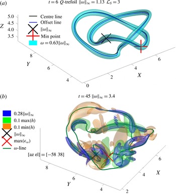
(a) Vorticity isosurface plus two closed vortex lines seeded near
 $\Vert \unicode[STIX]{x1D714}\Vert _{\infty }$
(
 $\boldsymbol{\times }$
) of the perturbed trefoil vortex at
 $t=6$
. The red
 $\boldsymbol{ + }$
point is where reconnection will begin, with
 $h<0$
forming to its left. (b) At
 $t=45$
, just after the first reconnection ends, a gap between strong
 $h<0$
(yellow, left) and strong
 $h>0$
(green, right) forms to the right of the red
 $\boldsymbol{\times }$
at the maximum dissipation of enstrophy
 $\max (\unicode[STIX]{x1D716}_{\unicode[STIX]{x1D714}})$
(1.5). Note that the vortex trajectory now avoids this gap. Further details on the evolution of the structure for
 $6\leqslant t\leqslant 45$
, including the details of the vorticity at
 $t=t_{x}=40$
, are in Kerr (Reference Kerr2018). © The Japan Society of Fluid Mechanics. Reproduced by permission of IOP Publishing. All rights reserved.

1.1 Equations and norms
The governing equations are the incompressible Navier–Stokes equations on a three-dimensional torus
 $\mathbb{T}_{\ell }^{3}$
, a periodic box with volume
 $V=\ell ^{3}$
,
 $$\begin{eqnarray}\displaystyle \left.\begin{array}{@{}c@{}}\boldsymbol{u}_{t}-\unicode[STIX]{x1D708}\unicode[STIX]{x0394}\boldsymbol{u}+(\boldsymbol{u}\boldsymbol{\cdot }\unicode[STIX]{x1D735})\boldsymbol{u}+\unicode[STIX]{x1D735}p=0\\ \unicode[STIX]{x1D735}\boldsymbol{\cdot }\boldsymbol{u}=0\end{array}\right\}\quad \text{in}~\mathbb{T}_{\ell }^{3}\times [0,T), & & \displaystyle\end{eqnarray}$$
and the numerical method will be
 $2/3$
rds-dealiased pseudo-spectral code with a high-wavenumber cutoff filter (Kerr Reference Kerr2013a
).
With
 $\unicode[STIX]{x1D74E}=\unicode[STIX]{x1D735}\times \boldsymbol{u}$
the vorticity, the diagnostics equations for the densities of the energy
 $e=(1/2)|\boldsymbol{u}|^{2}$
, enstrophy
 $|\unicode[STIX]{x1D74E}|^{2}$
and helicity
 $h=\boldsymbol{u}\boldsymbol{\cdot }\unicode[STIX]{x1D74E}$
, along with their volume-integrated norms
 $E$
,
 $Z$
and
 ${\mathcal{H}}$
, are
 $$\begin{eqnarray}\displaystyle \frac{\unicode[STIX]{x2202}e}{\unicode[STIX]{x2202}t}+(\boldsymbol{u}\boldsymbol{\cdot }\unicode[STIX]{x1D735})e=-\unicode[STIX]{x1D735}\boldsymbol{\cdot }(\boldsymbol{u}p)+\unicode[STIX]{x1D708}\unicode[STIX]{x0394}e-\underbrace{\unicode[STIX]{x1D708}(\unicode[STIX]{x1D735}\boldsymbol{u})^{2}}_{\unicode[STIX]{x1D716}=\text{dissipation}},\quad E=\frac{1}{2}\int \boldsymbol{u}^{2}\,\text{d}V, & & \displaystyle\end{eqnarray}$$
 $$\begin{eqnarray}\displaystyle \frac{\unicode[STIX]{x2202}|\unicode[STIX]{x1D74E}|^{2}}{\unicode[STIX]{x2202}t}+(\boldsymbol{u}\boldsymbol{\cdot }\unicode[STIX]{x1D735})|\unicode[STIX]{x1D74E}|^{2}=\underbrace{2\unicode[STIX]{x1D74E}\boldsymbol{S}\unicode[STIX]{x1D74E}}_{Z_{p}=\text{production}}+\,\unicode[STIX]{x1D708}\unicode[STIX]{x0394}|\unicode[STIX]{x1D74E}|^{2}-\underbrace{2\unicode[STIX]{x1D708}(\unicode[STIX]{x1D735}\unicode[STIX]{x1D74E})^{2}}_{\unicode[STIX]{x1D716}_{\unicode[STIX]{x1D714}}},\quad Z=\int \unicode[STIX]{x1D74E}^{2}\,\text{d}V, & & \displaystyle\end{eqnarray}$$
where
 $\boldsymbol{S}=(1/2)(\unicode[STIX]{x1D735}\boldsymbol{u}+\unicode[STIX]{x1D735}\boldsymbol{u}^{\text{T}})$
is the strain, and
 $$\begin{eqnarray}\displaystyle \frac{\unicode[STIX]{x2202}h}{\unicode[STIX]{x2202}t}+(\boldsymbol{u}\boldsymbol{\cdot }\unicode[STIX]{x1D735})h=\underbrace{-\unicode[STIX]{x1D74E}\boldsymbol{\cdot }\unicode[STIX]{x1D735}\unicode[STIX]{x1D6F1}}_{\unicode[STIX]{x1D714}\text{-}\text{transport}}+\,\unicode[STIX]{x1D708}\unicode[STIX]{x0394}h-\underbrace{2\unicode[STIX]{x1D708}\text{tr}(\unicode[STIX]{x1D735}\unicode[STIX]{x1D74E}\boldsymbol{\cdot }\unicode[STIX]{x1D735}\boldsymbol{u}^{\text{T}})}_{\unicode[STIX]{x1D716}_{h}={\mathcal{H}}\text{-}\text{dissipation}},\quad {\mathcal{H}}=\int \boldsymbol{u}\boldsymbol{\cdot }\unicode[STIX]{x1D74E}\,\text{d}V, & & \displaystyle\end{eqnarray}$$
where
 $\unicode[STIX]{x1D6F1}=p-(1/2)\boldsymbol{u}^{2}\neq p_{h}$
, the pressure head
 $p_{h}=p+(1/2)\boldsymbol{u}^{2}$
. The energy dissipation rate is
 $\unicode[STIX]{x1D716}(t)=\unicode[STIX]{x1D708}Z$
and changes in the energy up to
 $t=T$
are given by
 $$\begin{eqnarray}\displaystyle \unicode[STIX]{x0394}E(T)=E(0)-E(T)=\int _{0}^{T}\unicode[STIX]{x1D716}\,\text{d}t=\int _{0}^{T}\unicode[STIX]{x1D708}Z\,\text{d}t. & & \displaystyle\end{eqnarray}$$
The inviscid
 $\unicode[STIX]{x1D708}=0$
equations conserve
 $E$
and
 ${\mathcal{H}}$
, produce
 $Z$
from the local
 $Z_{p}$
(1.5) and can transport the local helicity along vortex lines (1.6). With
 $\unicode[STIX]{x1D708}\neq 0$
, the viscous energy dissipation rate is
 $\unicode[STIX]{x1D716}=\unicode[STIX]{x1D708}Z>0$
(1.4), the local enstrophy dissipation is
 $\unicode[STIX]{x1D716}_{\unicode[STIX]{x1D714}}>0$
(1.5), and the local helicity density dissipation
 $\unicode[STIX]{x1D716}_{h}$
(1.6) can be of either sign, resulting in the regions of small-scale helicity of both signs about the reconnection in figure 1(b). Additional volume-integrated diagnostics include Lebesgue measures and Sobolev norms using the wavenumbers
 $\boldsymbol{k}$
, which are respectively
 $$\begin{eqnarray}\displaystyle \Vert u\Vert _{L_{\ell }^{p}}^{}=\left(\int _{\mathbb{T}_{\ell }^{3}}\text{d}\unicode[STIX]{x1D6FA}|\boldsymbol{u}|^{p}\right)^{1/p}\quad \text{and}\quad H_{\ell }^{(\bullet s)}=\Vert u\Vert _{\overset{\boldsymbol{\cdot }}{H}_{\ell }^{s}}^{}=\left(\frac{\ell }{(2\unicode[STIX]{x03C0})}\right)^{3/2}\left(\sum |\boldsymbol{k}|^{2s}|\hat{\boldsymbol{u}}(\boldsymbol{k})|^{2}\right)^{1/2}. & & \displaystyle \nonumber\\ \displaystyle & & \displaystyle\end{eqnarray}$$
Those plotted are
 $H_{\ell }^{(\bullet 1/2)}=\Vert u\Vert _{\overset{\boldsymbol{\cdot }}{H}_{\ell }^{1/2}}^{}$
, the enstrophy
 $Z=(H_{\ell }^{(\bullet 1)})^{2}=\Vert \unicode[STIX]{x1D714}\Vert _{L_{\ell }^{2}}^{2}$
, the maximum of vorticity
 $\Vert \unicode[STIX]{x1D714}\Vert _{\infty }^{}=\sup |\unicode[STIX]{x1D714}|=\Vert \unicode[STIX]{x1D714}\Vert _{L_{\ell }^{\infty }}^{}$
(for all
 $\ell$
) and the cubic velocity norm
 $\Vert u\Vert _{L_{\ell }^{3}}^{}$
.
1.2 Initial conditions
To initialise the trefoils and anti-parallel vortices, their trajectories were mapped onto their respective three-dimensional computational meshes following the method introduced by Kerr (Reference Kerr2013a ). This used the minimum distances between the mesh points and the trajectories in smoothed point-vortex profiles to suppress the unphysical internal instabilities of the Melander & Hussain (Reference Melander and Hussain1989) initial condition.
The modifications required to map the vorticity of the doubly looped trefoils, with the topology of (2,3) knots, are described in Kerr (Reference Kerr2018). This includes the additional, weak vortex rings on the periphery that are used to ensure that there is a single, dominant reconnection event as in the experiments of Kleckner & Irvine (Reference Kleckner and Irvine2013) and Scheeler et al. (Reference Scheeler, Kleckner, Proment, Kindlmann and Irvine2014). This initialisation also ensures that the trefoils’ vorticity diagnostics, the global helicity and the
 $\Vert u\Vert _{L_{\ell }^{3}}^{}$
norm all converge rapidly as the domain is increased. The total energy also converges to an upper bound, but more slowly. This means the initial condition has ‘compact support’, an assumption often made in the analysis of the Navier–Stokes equations.
The resulting state shortly after
 $t=0$
is in figure 1(a). Besides the vorticity isosurface of the trefoil, the position
 $\boldsymbol{x}_{\infty }$
of the maximum of vorticity
 $\Vert \unicode[STIX]{x1D714}\Vert _{\infty }$
, a red
 $\boldsymbol{ + }$
at one of the points of closest approach of the two loops and two vortex trajectories
 $\boldsymbol{x}_{i}(s)$
and
 $\boldsymbol{x}_{j}(s)$
are indicated. The two trajectories verify that the self-linking number
 ${\mathcal{L}}_{S}=3$
, where
 ${\mathcal{L}}_{S}={\mathcal{L}}_{ij}/2$
and
 ${\mathcal{L}}_{ij}$
is the Gauss linking integral for
 $\boldsymbol{x}_{i}$
and
 $\boldsymbol{x}_{j}$
:
 $$\begin{eqnarray}\displaystyle {\mathcal{L}}_{ij}=\mathop{\sum }_{ij}\frac{1}{4\unicode[STIX]{x03C0}}\oint _{{\mathcal{C}}_{i}}\oint _{{\mathcal{C}}_{j}}\frac{(\text{d}\boldsymbol{x}_{i}\times \text{d}\boldsymbol{x}_{j})\boldsymbol{\cdot }(\boldsymbol{x}_{i}-\boldsymbol{x}_{j})}{(|\boldsymbol{x}_{i}-\boldsymbol{x}_{j}|^{2})^{1.5}}. & & \displaystyle\end{eqnarray}$$
This gives
 ${\mathcal{L}}_{S}=3$
and, for a circulation of
 $\unicode[STIX]{x1D6E4}=0.505$
, both the predicted helicity of
 ${\mathcal{H}}=\unicode[STIX]{x1D6E4}^{2}{\mathcal{L}}_{S}$
(Moffatt & Ricca Reference Moffatt and Ricca1992) and the directly determined global helicity (1.6) are
 ${\mathcal{H}}\approx 7.7\times 10^{-4}$
at
 $t=0$
.
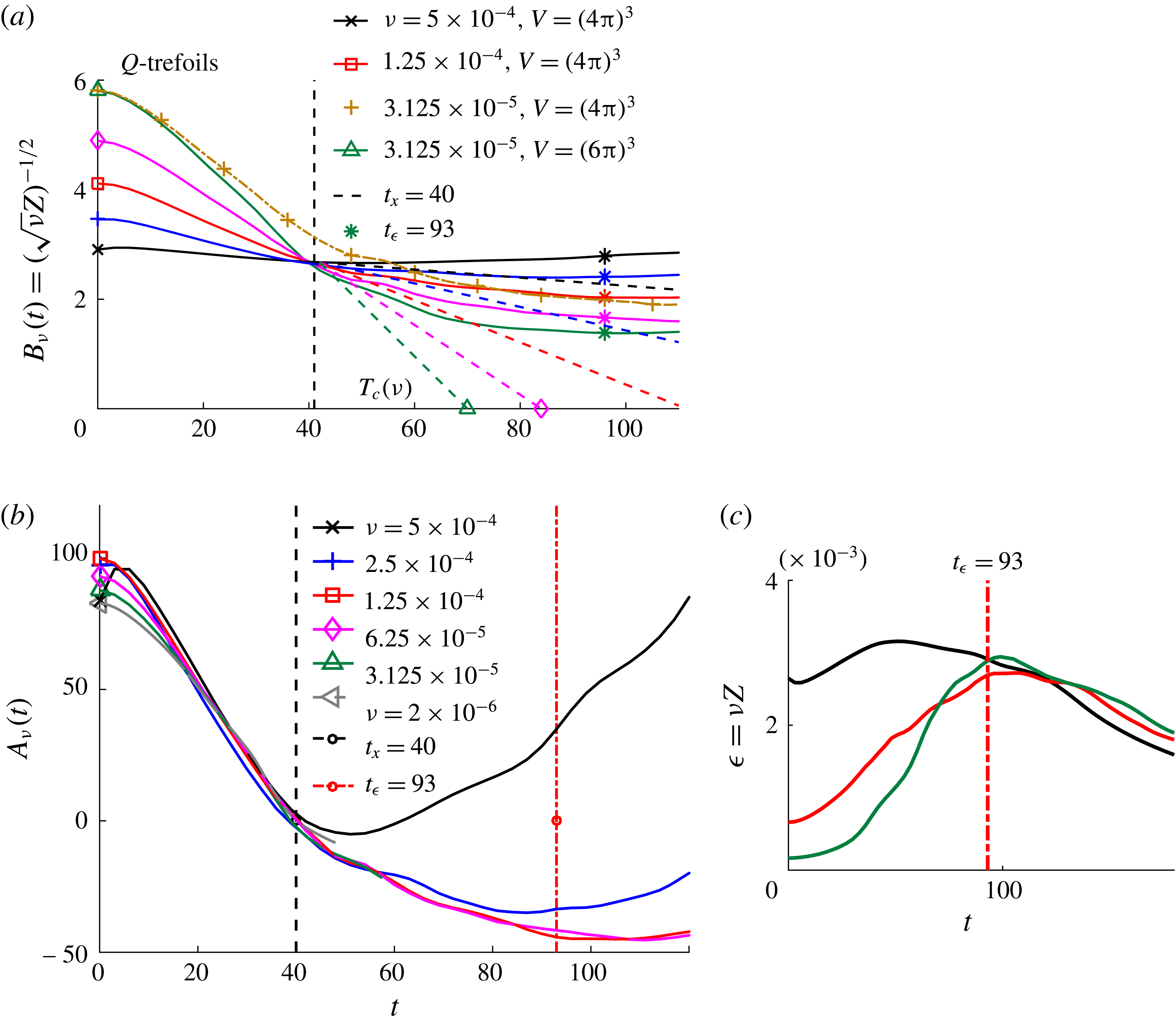
(a) Scaling of
 $B_{\unicode[STIX]{x1D708}}(t)$
(1.1) beginning at
 $t_{r}\approx 15$
. The
 $\ast$
indicate when the energy dissipation rates
 $\unicode[STIX]{x1D716}=\unicode[STIX]{x1D708}Z$
saturate at a common time
 $t_{\unicode[STIX]{x1D716}}$
. The dashed lines indicate the critical times
 $T_{c}(\unicode[STIX]{x1D708})$
(2.1) that are obtained by extrapolating
 $B_{\unicode[STIX]{x1D708}}(t)$
from a common early time of
 $t_{r}$
through
 $t_{x}$
to
 $B_{\unicode[STIX]{x1D708}}^{{\sim}}(T_{c})=0$
. (b) Evolution of the inverse, temporally scaled enstrophy
 $A_{\unicode[STIX]{x1D708}}(t)$
created by using
 $T_{c}(\unicode[STIX]{x1D708})$
in (2.2). (c) The energy dissipation rates
 $\unicode[STIX]{x1D716}=\unicode[STIX]{x1D708}Z$
(1.4) for different
 $\unicode[STIX]{x1D708}$
cross at
 $t_{\unicode[STIX]{x1D716}}=93$
, but without any clear scaling for
 $t_{x}\leqslant t\leqslant t_{\unicode[STIX]{x1D716}}$
.

The red
 $\boldsymbol{ + }$
, indicating the loops’ closest approach, is where reconnection starts at
 $t_{r}\approx 15$
, as discussed in § 4, and then continues until a clear gap appears in the
 $t=45$
frame in figure 1(b), for which the intermediate steps are discussed in Kerr (Reference Kerr2018).
Kerr (Reference Kerr2018) used two trefoil configurations, Q and S. These had the same trajectories and circulations, but different effective core radii
 $r_{e}$
, and as long as the domain sizes
 $\ell$
were increased as
 $\unicode[STIX]{x1D708}$
decreased, both had similar linearly decreasing
 $B_{\unicode[STIX]{x1D708}}(t)$
regimes that crossed at
 $t_{x}\approx 40$
. Finding that
 $t_{x}$
is independent of
 $r_{e}$
and
 $\unicode[STIX]{x1D708}$
shows that the most important time scale is the nonlinear time scale formed by the circulation
 $\unicode[STIX]{x1D6E4}$
and size of the trefoils. Only the Q-trefoils, previously compared to the Kleckner & Irvine (Reference Kleckner and Irvine2013) experiment, are used here. The domains used are given in the legends of figures 2 and 5.
The new anti-parallel calculations are similar to those in Kerr (Reference Kerr2013a
) with mirror-symmetric boundaries used in
 $y$
and
 $z$
, but with domains that are shorter in
 $y$
and wider in
 $z$
. The circulations are
 $\pm 5$
and the separation of the vortices
 $\unicode[STIX]{x1D6FF}=4$
. The
 $\unicode[STIX]{x1D708}=2\times 10^{-3}$
,
 $1\times 10^{-3}$
and
 $5\times 10^{-4}$
cases are in
 $L_{x}\times L_{y}\times L_{z}=4\unicode[STIX]{x03C0}\times 4\unicode[STIX]{x03C0}\times 2\unicode[STIX]{x03C0}$
domains with
 $\unicode[STIX]{x1D708}=2\times 10^{-3}$
using a
 $512\times 512\times 512$
mesh and the
 $\unicode[STIX]{x1D708}=1\times 10^{-3}$
and
 $5\times 10^{-4}$
cases using up to
 $1024\times 1024\times 2048$
meshes to validate the calculations over
 $t>12$
. The
 $\unicode[STIX]{x1D708}=2.5\times 10^{-4}$
case is run in a larger
 $(4\unicode[STIX]{x03C0})^{3}$
domain on
 $2048^{3}$
meshes to validate the calculations for
 $t>8$
. For
 $\unicode[STIX]{x1D708}=1.25\times 10^{-4}$
, the domain is
 $L_{x}\times L_{y}\times L_{z}=4\unicode[STIX]{x03C0}\times 4\unicode[STIX]{x03C0}\times 8\unicode[STIX]{x03C0}$
with a
 $2048\times 2048\times 4096$
mesh used for the brief period
 $14\leqslant t\leqslant 18$
to ensure that the viscous circulation exchange
 $\unicode[STIX]{x1D716}_{\unicode[STIX]{x1D6E4}}$
(1.2) is converged. Due to the symmetries on the
 $y$
and
 $z$
boundaries, the
 $L_{x}\times L_{y}\times L_{z}$
computational domains are equivalent to
 $L_{x}\times 2L_{y}\times 2L_{z}$
fully periodic domains.
2 Path to identifying trefoil self-similar collapse
The steps taken to identify the self-similar collapse of the temporally scaled
 $B_{\unicode[STIX]{x1D708}}(t)$
(1.1) begin by plotting
 $B_{\unicode[STIX]{x1D708}}(t)=(\sqrt{\unicode[STIX]{x1D708}}Z(t))^{-1/2}$
(1.1) in figure 2(a). For all cases except one,
 $B_{\unicode[STIX]{x1D708}}(t_{x})\approx 2.6$
at
 $t=t_{x}\approx 40$
. The exception is the
 $\unicode[STIX]{x1D708}=3.125\times 10^{-5}$
orange
 $\boldsymbol{ + }$
curve with
 $\ell =4\unicode[STIX]{x03C0}$
. This case does not cross those with
 $\unicode[STIX]{x1D708}<3.125\times 10^{-5}$
unless
 $\ell =6\unicode[STIX]{x03C0}$
, shown in green.
This behaviour is general. That is, for
 $\unicode[STIX]{x1D708}=6.25\times 10^{-5}$
, its
 $B_{\unicode[STIX]{x1D708}}(t_{x})\approx 2.6$
crosses the
 $\unicode[STIX]{x1D708}<6.25\times 10^{-5}$
,
 $\ell =3\unicode[STIX]{x03C0}$
cases at
 $t=t_{x}=40$
only if a
 $\ell \geqslant 4\unicode[STIX]{x03C0}$
domain is used. How
 $\ell$
increases as
 $\unicode[STIX]{x1D708}$
decreases for
 $\unicode[STIX]{x1D708}<3.125\times 10^{-5}$
is given in the legend of figure 5(c). The case with
 $\unicode[STIX]{x1D708}=2\times 10^{-6}$
and
 $\ell =12\unicode[STIX]{x03C0}$
is included in figure 2(b) to demonstrate the robustness of the collapse even when
 $\unicode[STIX]{x1D708}$
has decreased by a factor of 256 and the calculation is under-resolved in terms of
 $\Vert \unicode[STIX]{x1D714}\Vert _{\infty }$
for
 $t\geqslant 25$
, as indicated in figure 5.
Self-similar collapse is obtained by extrapolating the linear
 $B_{\unicode[STIX]{x1D708}}(t)$
range for
 $t\lesssim t_{x}$
to critical times
 $T_{c}(\unicode[STIX]{x1D708})$
defined by
 $$\begin{eqnarray}\displaystyle T_{c}(\unicode[STIX]{x1D708})=(t_{x}-t_{r}B_{x}/B_{\unicode[STIX]{x1D708}}(t_{r}))/(1-B_{x}/B_{\unicode[STIX]{x1D708}}(t_{r})). & & \displaystyle\end{eqnarray}$$
The
 $T_{c}(\unicode[STIX]{x1D708})$
can then be used to define the self-similar collapse plotted in figure 2(b) using:
 $$\begin{eqnarray}\displaystyle A_{\unicode[STIX]{x1D708}}(t)=(T_{c}(\unicode[STIX]{x1D708})-t_{x})(B_{\unicode[STIX]{x1D708}}(t)-B_{x}). & & \displaystyle\end{eqnarray}$$
This collapse begins as reconnection starts at
 $t_{r}\approx 15$
, identified in § 4 as when several maxima markers shift to the vicinity of the closest approach of the two loops. The relative positions of that point and
 $\Vert \unicode[STIX]{x1D714}(\boldsymbol{x}_{\infty })\Vert _{\infty }$
persist from their positions at
 $t=6$
in figure 1(a) until
 $t>t_{x}=40$
, as in figure 1(b). A side benefit of the collapse to early times is that this justifies making a connection between the very small
 $\unicode[STIX]{x1D708}$
, early-time analysis in figure 5 and the dynamics at
 $t=t_{x}=40$
.
What is the physical significance of
 $t_{x}$
? Kerr (Reference Kerr2018) concluded that the first reconnection ended with the formation of a very localised gap in the trefoil structure at
 $t_{x}=40$
. Because the best indication of when reconnection ends for the experiments is when gaps form in their macroscopic vortex structures, figure 1(b) at
 $t=45$
is shown because that is the first time that the trefoil’s macroscopic structure has a gap, indicated by the gap in the vorticity isosurface to the right of the red
 $\boldsymbol{\times }$
, which indicates the position of
 $\max (\unicode[STIX]{x1D716}_{\unicode[STIX]{x1D714}})$
(1.5). This is also why, for the anti-parallel simulations,
 $t=24$
is shown in figure 3.
The
 $t=45$
trefoil gap is between an intensifying
 $h>0$
isosurface with growing
 $|\unicode[STIX]{x1D714}|^{2}$
and dissipation on its right, that continues for
 $t>45$
, and an
 $h<0$
isosurface on its left, with the vortex trajectory avoiding the gap entirely. These oppositely signed regions of helicity are tied to the helicity dissipation terms in (1.6). There is also growing
 $h<0$
along the upper left, outer loop of the trefoil. This
 $h<0$
zone begins to the left of
 $\Vert \unicode[STIX]{x1D714}\Vert _{\infty }$
, appears very weakly even at
 $t=6$
, before reconnection truly begins, and is the first region to feel the effect of the periodic boundaries.
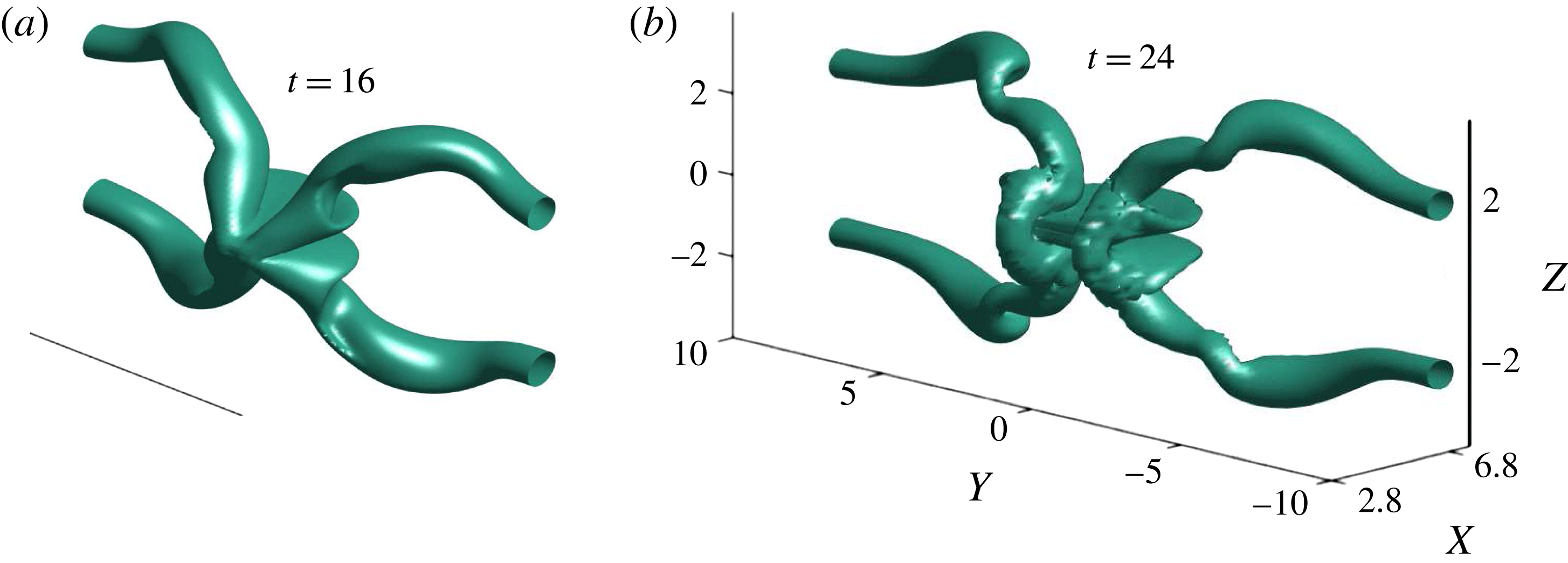
Three-dimensional isosurfaces of the anti-parallel vortices at
 $t=16$
and
 $t=24$
showing the evolution from flattening across the
 $z=0$
plane to the formation of a gap between the new vorticity that crosses the
 $z=0$
plane, with significant twisting on the arms that extend far, in
 $z$
, from the
 $y=z=0$
line in
 $x$
. Extensions that require increases in
 $L_{z}$
as
 $\unicode[STIX]{x1D708}$
decreases.

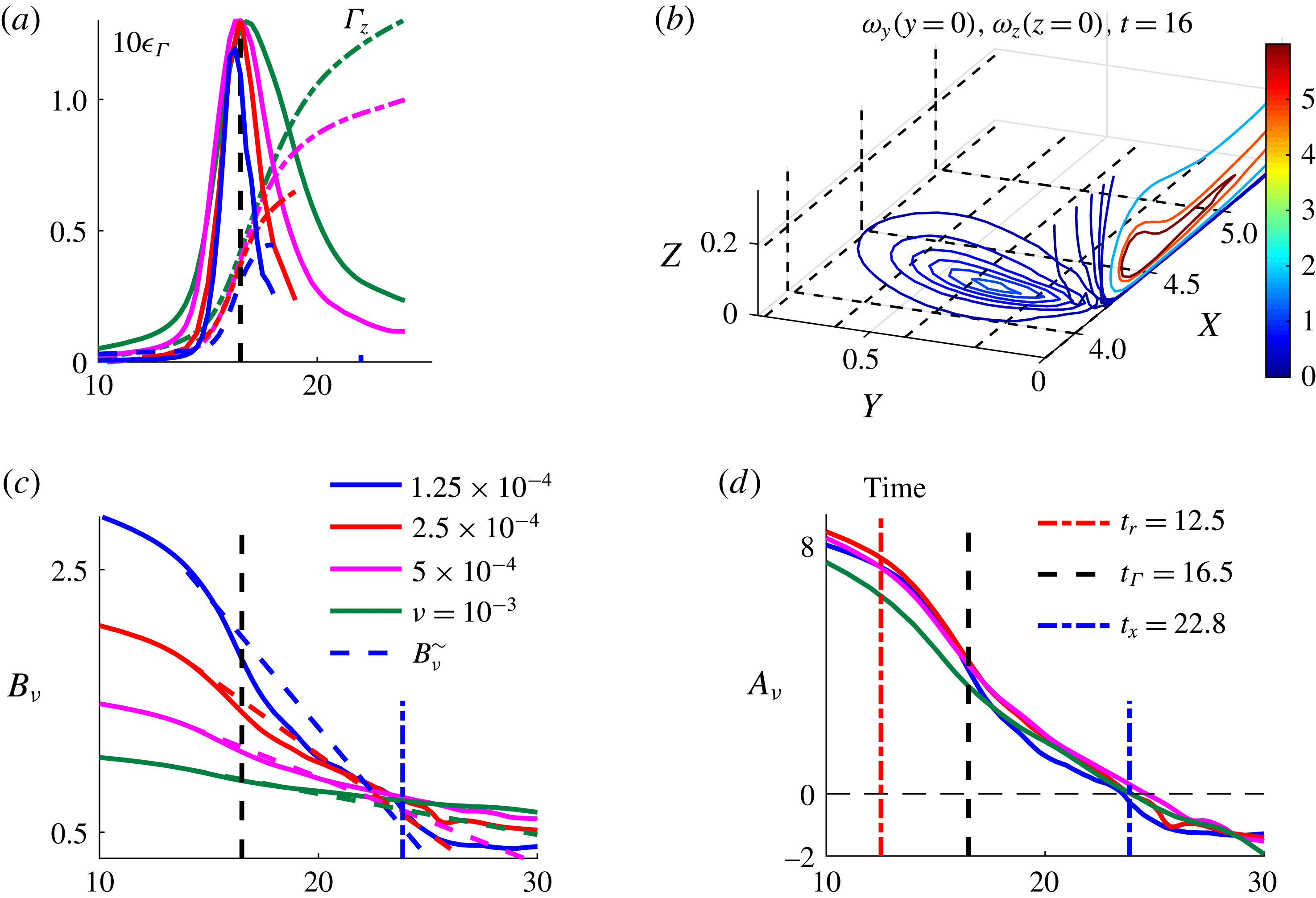
Diagnostics for the anti-parallel calculations during the first reconnection. (a) The growth of
 $\unicode[STIX]{x1D6E4}_{z}(t)$
(mirrored by the decay of
 $\unicode[STIX]{x1D6E4}_{y}(0)=4.6$
) and the collapse of
 $\unicode[STIX]{x1D716}_{\unicode[STIX]{x1D6E4}}$
(1.2), the circulation exchange between the symmetry planes, both of which first become noticeable at
 $t\approx 14$
. (b) Contours of
 $\unicode[STIX]{x1D714}_{y}$
on the
 $y=0$
plane and
 $\unicode[STIX]{x1D714}_{z}$
on the
 $z=0$
plane at
 $t=16$
. (c)
 $B_{\unicode[STIX]{x1D708}}(t)$
and the
 $B_{\unicode[STIX]{x1D708}}^{{\sim}}(t)$
dashed lines that are extrapolated from tangents at
 $B_{\unicode[STIX]{x1D708}}|_{t=14}$
, with both sets of curves converging near
 $t_{x}=22.85$
with
 $B_{\unicode[STIX]{x1D708}}(t_{x})\approx 0.73$
. (d)
 $A_{\unicode[STIX]{x1D708}}(t)$
(2.2) collapse between when the
 $\Vert u\Vert _{\infty }$
position shifts to the
 $y=z=0$
line at
 $t_{r}=12.5$
and
 $t_{x}$
, when the
 $B_{\unicode[STIX]{x1D708}}^{{\sim}}(t)$
cross.

3 Self-similar anti-parallel collapse
The new anti-parallel calculations in figure 3 are the second set of calculations showing collapse. The period to be considered is shown by the
 $t=16$
and
 $t=24$
isosurfaces in figure 3, which roughly represent the beginning and the end of the first reconnection. The
 $t=16$
isosurfaces are similar to those in many earlier Euler and early-time Navier–Stokes papers with vortex flattening about the
 $z=0$
plane, while the
 $t=24$
vertical isosurfaces have a gap through the
 $z=0$
plane and spirals extending along the arms. The gap indicates the end of the first phase of reconnection, while the spirals induce later reconnection events as discussed in Kerr (Reference Kerr2013a
).
How do the anti-parallel rescaled enstrophies
 $B_{\unicode[STIX]{x1D708}}(t)$
behave? These are given in figure 4(c), with a change in behaviour at
 $t\approx 16$
for all four values of
 $\unicode[STIX]{x1D708}$
as reconnection begins and a convergence of the solid lines at
 $t\approx 25$
as the gap forms in the vorticity isosurface.
However, unlike the trefoils in figure 2(a), these
 $B_{\unicode[STIX]{x1D708}}(t)$
do not decrease linearly, so another method is needed to find
 $t_{x}$
,
 $T_{c}(\unicode[STIX]{x1D708})$
and
 $A_{\unicode[STIX]{x1D708}}(t)$
. The first step in figure 4(a) is to plot the
 $t\sim 16$
,
 $\unicode[STIX]{x1D708}\leqslant 1\times 10^{-3}$
circulations
 $\unicode[STIX]{x1D6E4}_{z}$
on the
 $x$
–
 $y$
symmetry plane and the following integral of the dissipative terms along the
 $y=z=0$
line (Virk et al.
Reference Virk, Hussain and Kerr1995).
This is the viscous circulation exchange
 $\unicode[STIX]{x1D716}_{\unicode[STIX]{x1D6E4}}(t)$
(1.2) between
 $\unicode[STIX]{x1D6E4}_{y}$
on the
 $x{-}z$
symmetry plane and
 $\unicode[STIX]{x1D6E4}_{z}$
on the
 $x$
–
 $y$
symmetry plane, as illustrated in figure 4(b) with contours of
 $\unicode[STIX]{x1D714}_{y}$
and
 $\unicode[STIX]{x1D714}_{z}$
in the symmetry planes.
Significantly, the
 $\unicode[STIX]{x1D716}_{\unicode[STIX]{x1D6E4}}(t)$
have a
 $\unicode[STIX]{x1D708}$
-independent collapse that begins at
 $t\approx 14>t_{r}\approx 12.5$
, where
 $t_{r}$
is defined in § 4, and lasts to
 $t_{\unicode[STIX]{x1D6E4}}\approx 16.5$
, the time with maximum
 $\unicode[STIX]{x1D716}_{\unicode[STIX]{x1D6E4}}$
, when the growing
 $\unicode[STIX]{x1D6E4}_{z}(t)$
for different
 $\unicode[STIX]{x1D708}$
cross and by which there is a small, but finite, exchange of circulation
 $\unicode[STIX]{x0394}\unicode[STIX]{x1D6E4}=\unicode[STIX]{x1D6E4}_{z}(t_{\unicode[STIX]{x1D6E4}})$
in figure 4(a), and an exchange becomes the visible gap in figure 3(b) at
 $t=24$
. Over this brief period, the exchange is consistent with singular Leray scaling (6.3) (Leray Reference Leray1934) and is suppressed if the domain size, particularly in
 $z$
, is not increased as
 $\unicode[STIX]{x1D708}$
decreases, as for the two
 $\unicode[STIX]{x1D708}=3.125\times 10^{-5}$
trefoil
 $B_{\unicode[STIX]{x1D708}}(t)$
curves in figure 2(a).
Once the
 $\unicode[STIX]{x1D716}_{\unicode[STIX]{x1D6E4}}(t)$
collapse phase was identified, it was realised that the
 $B_{\unicode[STIX]{x1D708}}(t)$
do linearly decay, but only for the brief period
 $(t_{r}=12.5)\leqslant t\leqslant (t_{\unicode[STIX]{x1D6E4}}=16.5)$
. These can easily be extrapolated to
 $t>t_{\unicode[STIX]{x1D6E4}}=16.5$
to form extrapolated
 $B_{\unicode[STIX]{x1D708}}^{{\sim}}(t)$
, dashed lines in figure 4(c), from which
 $t_{x}=22.85$
can be defined as when the
 $B_{\unicode[STIX]{x1D708}}^{{\sim}}$
cross and the
 $T_{c}(\unicode[STIX]{x1D708})$
(2.1) as when
 $B_{\unicode[STIX]{x1D708}}^{{\sim}}(T_{c})=0$
. Together in (2.2) with the
 $B_{\unicode[STIX]{x1D708}}(t)$
, these define the
 $A_{\unicode[STIX]{x1D708}}(t)$
that collapse for
 $t_{r}\leqslant t\leqslant t_{x}$
and a bit more in time in figure 4(d), even if this collapse is not linear.
Besides showing how the exchange of circulation kick starts reconnection, the period of anti-parallel reconnection also provides a link to periods of intense enstrophy growth in more traditional turbulence calculations. This was done by determining higher-order vorticity moments
 $\Vert \unicode[STIX]{x1D714}\Vert _{L_{\ell }^{p}}^{}$
, which when rescaled as suggested by Gibbon (Reference Gibbon2010, Reference Gibbon2012) are invariably inversely ordered from the Hölder (5.3) expectation (Donzis et al.
Reference Donzis, Gibbon, Gupta, Kerr, Pandit and Vincenzi2013). The case where this ordering is strongest is an earlier version of the anti-parallel calculation here.
4 Identifying when self-similar collapse begins and ends
While the end of the
 $A_{\unicode[STIX]{x1D708}}(t)$
collapse in both configurations is indicated physically by the clear gaps in the three-dimensional vorticity isosurfaces and the
 $A_{\unicode[STIX]{x1D708}}(t)$
curves suggest that the reconnections begin at
 $t_{r}\approx 15$
for the trefoils and
 $t_{r}\sim 12.5{-}14$
for the anti-parallel vortices, consistent visual signals from the graphics indicating when physical reconnection begins could not be identified.
A different approach for identifying the
 $t_{r}$
, without using three-dimensional structural clues, was suggested by the anti-parallel simulations after it was noticed that the positions of the maxima of vorticity and velocity suddenly shift at
 $t\approx 12.5$
. At
 $t=0$
,
 $\Vert \unicode[STIX]{x1D714}\Vert _{\infty }$
is on the
 $x{-}z$
perturbation plane and
 $\Vert u\Vert _{\infty }$
is outside it. Then at
 $t\approx 12.5$
,
 $\Vert u\Vert _{\infty }$
moves to the
 $y=z=0$
line and
 $\Vert \unicode[STIX]{x1D714}\Vert _{\infty }$
moves off the
 $x{-}z$
perturbation plane.
On that basis, for the trefoils, the positions of
 $\Vert \unicode[STIX]{x1D714}\Vert _{\infty }$
,
 $\Vert u\Vert _{\infty }$
and the minimum and maximum of the helicity have been tracked in time. While the relative positions of
 $\Vert \unicode[STIX]{x1D714}\Vert _{\infty }$
and the closest approach of the trefoil loops, as in figure 1(a), remain the same for
 $t<t_{x}$
, the positions of
 $\Vert u\Vert _{\infty }$
and the minimum and maximum of the helicity all shift to the vicinity of the closest approach at
 $t\approx 15$
, with these shifts providing a quantitative diagnostic for when the trefoils’ reconnection begins.
Are the periods of reconnection and
 $A_{\unicode[STIX]{x1D708}}(t)$
collapse, that is
 $t_{x}-t_{r}$
, similar multiples of the nonlinear time scale
 $t_{\unicode[STIX]{x1D6FF}}=\unicode[STIX]{x1D6FF}^{2}/\unicode[STIX]{x1D6E4}$
? For the anti-parallel vortices,
 $t_{x}-t_{r}\sim 10\approx 3t_{\unicode[STIX]{x1D6FF}}\sim t_{r}$
. However, for the trefoils it is longer,
 $t_{x}-t_{r}\sim 25\sim 12t_{\unicode[STIX]{x1D6FF}}$
, as if the growth of
 $Z$
is in slow motion due to the strong helicity. Post-reconnection, the dissipation rates
 $\unicode[STIX]{x1D716}=\unicode[STIX]{x1D708}Z$
continue to grow, with the trefoils’
 $\unicode[STIX]{x1D716}$
curves crossing weakly at
 $t_{\unicode[STIX]{x1D716}}\approx 2t_{x}=93$
in figure 2(c) and weakly suggesting that the dissipation integral
 $\unicode[STIX]{x0394}E$
(1.7) might stay large as the viscosity
 $\unicode[STIX]{x1D708}$
decreases. For the anti-parallel calculations, the
 $\unicode[STIX]{x1D716}$
do not converge over the simulated period at all.
5 Mathematics underlying increasing the domain
Why must the domain be increased as the viscosity is decreased? The physical explanation proposed by Kerr (Reference Kerr2018) is that if the domain was too small, the trefoil can interact with itself across the periodic boundaries, with a possible source being the negative helicity (orange isosurface) generated on the trefoil’s outer loop in figure 1(b). For the anti-parallel vortices, this interaction would be across the outer
 $z$
-boundaries due to outer twists like those in figure 3(b).
A plausible mathematical reason comes from considering the following question (Constantin Reference Constantin1986). As
 $\unicode[STIX]{x1D708}$
decreases in a fixed periodic domain, could there be critical viscosities
 $\unicode[STIX]{x1D708}_{s}$
such that for
 $\unicode[STIX]{x1D708}<\unicode[STIX]{x1D708}_{s}$
the Navier–Stokes norms would be bounded by regular (non-singular) solutions of the
 $\unicode[STIX]{x1D708}=0$
Euler equations? What was shown is that the higher-order
 $s>5/2$
Sobolev norms of the differences, on a periodic box of size
 $\ell$
, between smooth solutions of the Euler
 $v(t)$
solutions for
 $0\leqslant \leqslant T$
and Navier–Stokes solutions
 $u(t)$
are bounded as
 $$\begin{eqnarray}\displaystyle \sup _{t\in [0,T]}\Vert u(t)-v(t)\Vert _{H_{\ell }^{s}}^{}\leqslant \unicode[STIX]{x1D708}\unicode[STIX]{x1D6FE}_{s}\quad \text{for all}~\unicode[STIX]{x1D708}\leqslant \unicode[STIX]{x1D708}_{s}(\ell )~\text{with}~\unicode[STIX]{x1D708}_{s}(\ell )\sim \ell ^{-2s+5}\unicode[STIX]{x1D704}_{s},s>5/2, & & \displaystyle\end{eqnarray}$$
where
 $\unicode[STIX]{x1D6FE}_{s}$
and
 $\unicode[STIX]{x1D704}_{s}$
are functions of the norms of the Euler solutions. The origin of the
 $\unicode[STIX]{x1D708}_{s}\sim \ell ^{-2s+5}$
scaling comes from a constant
 $c_{s}(\ell )\sim \ell ^{-5+2s}$
used in lowering the order of a
 $s+1$
term to order
 $s$
in the nonlinear time inequality of
 $(\text{d}/\text{d}t)\Vert u(t)-v(t)\Vert _{H_{\ell }^{s}}^{}$
(Constantin & Foias Reference Constantin and Foias1988) and the relevance of
 $\unicode[STIX]{x1D708}_{x}(\ell )$
to these calculations is that this scaling is consistent with how, empirically, the domain size
 $\ell$
increases as
 $\unicode[STIX]{x1D708}$
decreases, as given in the legend of figure 5.
To understand how these constants can depend upon
 $\ell$
and how the higher-order
 $\sup \Vert u(t)-v(t)\Vert _{H_{\ell }^{s}}^{}$
can bound the enstrophy
 $Z$
and restrict the
 $B_{\unicode[STIX]{x1D708}}(t)$
(1.1) scaling, consider the following example of how
 $\Vert \unicode[STIX]{x1D714}\Vert _{L_{\ell }^{2}}^{}=\sqrt{Z}$
can be bounded using a standard variation upon the Hölder inequality (Doering & Gibbon Reference Doering and Gibbon1995), taken to the
 $1/r$
power.
 $$\begin{eqnarray}\displaystyle \Vert fg\Vert _{L_{\ell }^{1}}^{1/r}\leqslant (\tilde{C}_{p}\Vert f\Vert _{p}^{})^{1/r}(\Vert g\Vert _{q}^{})^{1/r}\quad \text{for}~p^{-1}+q^{-1}=1. & & \displaystyle\end{eqnarray}$$
In
 $d=3$
dimensions, using
 $r=2$
,
 $g\equiv 1$
,
 $f=|\unicode[STIX]{x1D714}|^{r}$
,
 $p\rightarrow \infty$
and
 $q\rightarrow 1$
, which implies that
 $\Vert g\Vert _{1}^{}=\ell ^{d}=\ell ^{3}$
, one gets
 $$\begin{eqnarray}\displaystyle \Vert \unicode[STIX]{x1D714}\Vert _{L_{\ell }^{2}}^{}\leqslant C_{2}(\ell )\Vert \unicode[STIX]{x1D714}\Vert _{\infty }^{}\quad \text{with}~C_{2}(\ell )=\tilde{C}^{1/2}\ell ^{3/2}. & & \displaystyle\end{eqnarray}$$
Because
 $\Vert \unicode[STIX]{x1D714}(t)\Vert _{\infty }$
can be bounded by the higher-order
 $\sup \Vert u(t)-v(t)\Vert _{H_{\ell }^{s}}^{}$
using further
 $\ell$
-dependent Sobolev space embedding inequalities (Robinson et al.
Reference Robinson, Rodrigo and Sadowski2016), (5.1) and (5.3) can ensure that
 $Z$
is bounded and the following will be suppressed as
 $\unicode[STIX]{x1D708}\rightarrow 0$
: The decreasing
 $B_{\unicode[STIX]{x1D708}}(t)$
(1.1) scaling and dissipation growth
 $\unicode[STIX]{x1D716}=\unicode[STIX]{x1D708}Z$
in figure 2 and the
 $\unicode[STIX]{x1D716}_{\unicode[STIX]{x1D6E4}}$
(1.2) and
 $A_{\unicode[STIX]{x1D708}}(t)$
(2.2) collapse in figure 4.
However, for
 $\unicode[STIX]{x1D708}>\unicode[STIX]{x1D708}_{s}(\ell )$
, (5.1) poses no restrictions upon the growth of
 $Z$
, the
 $B_{\unicode[STIX]{x1D708}}(t)$
scaling and
 $\unicode[STIX]{x1D716}_{\unicode[STIX]{x1D6E4}}$
collapse so long as
 $\ell$
increases as
 $\unicode[STIX]{x1D708}$
decreases.
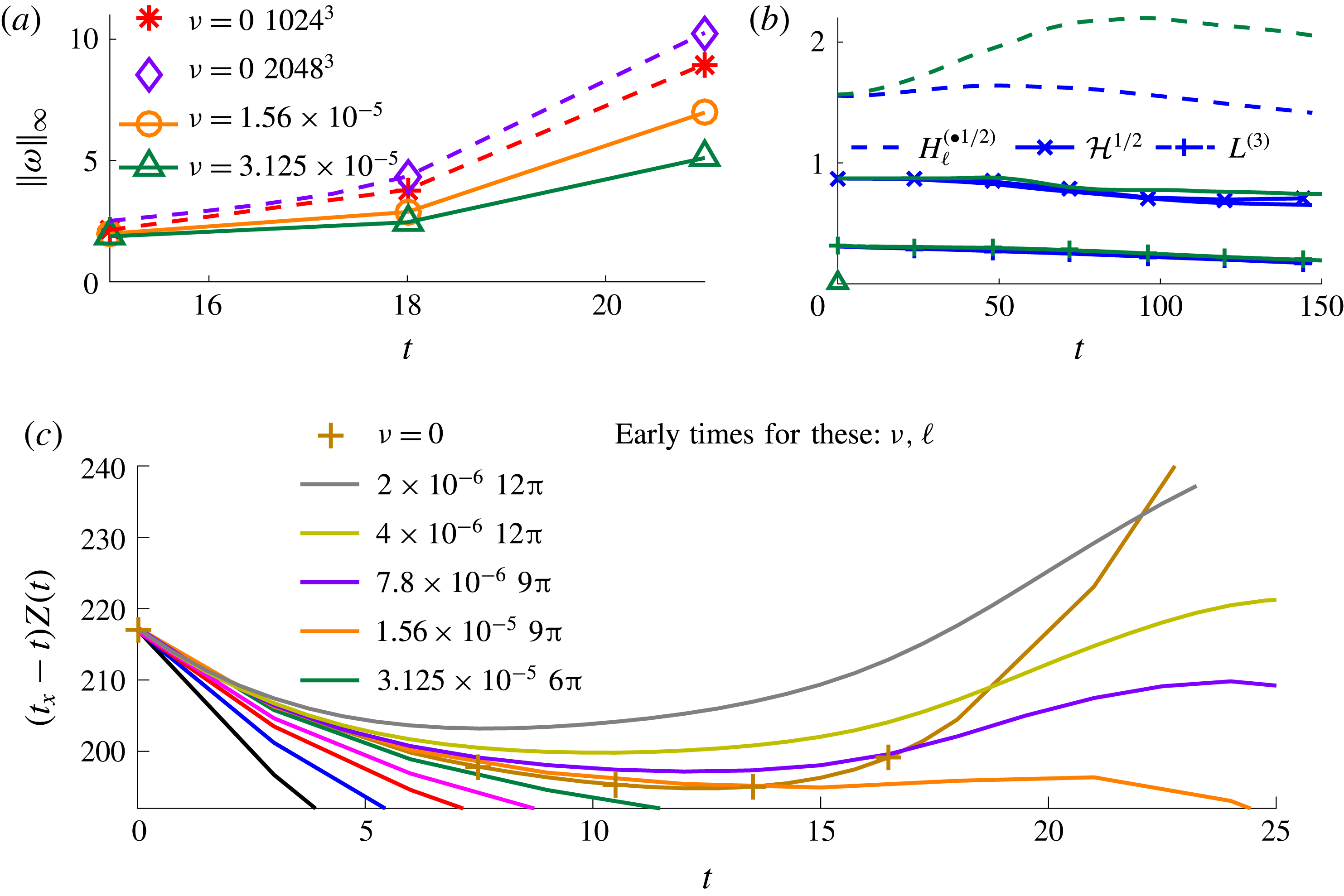
To address Navier–Stokes regularity more directly, several diagnostics are applied to the trefoil solutions in figure 5(a,b):
 $\Vert \unicode[STIX]{x1D714}\Vert _{\infty }$
,
 $H_{\ell }^{(\bullet 1/2)}$
,
 ${\mathcal{H}}^{1/2}$
and
 $L^{(3)}=\Vert u\Vert _{L^{3}}^{}$
. In figure 5(a), Navier–Stokes and Euler
 $\Vert \unicode[STIX]{x1D714}\Vert _{\infty }$
(Beale et al.
Reference Beale, Kato and Majda1984) are compared at early times,
 $t\leqslant 25$
, when both the
 $\unicode[STIX]{x1D708}\equiv 0$
Euler and the
 $\unicode[STIX]{x1D708}<3.125\times 10^{-5}$
calculations are resolved. Two
 $\ell ^{3}=(4\unicode[STIX]{x03C0})^{3}$
Euler
 $\Vert \unicode[STIX]{x1D714}\Vert _{\infty }$
curves are given, with an additional
 $\Vert \unicode[STIX]{x1D714}\Vert _{\infty }$
curve from an
 $\ell ^{3}=(9\unicode[STIX]{x03C0})^{3}$
,
 $2048^{3}$
calculation lying underneath the
 $(4\unicode[STIX]{x03C0})^{3}$
,
 $1024^{3}$
calculation with roughly the same local resolution. That overlaying demonstrates that the discretisation error is independent of the domain size
 $\ell$
once
 $\ell \geqslant 4\unicode[STIX]{x03C0}$
.
(a) Early-time
 $\Vert \unicode[STIX]{x1D714}\Vert _{\infty }$
for
 $\unicode[STIX]{x1D708}=0$
(Euler),
 $\unicode[STIX]{x1D708}=1.56\times 10^{-5}$
and
 $\unicode[STIX]{x1D708}=3.125\times 10^{-5}$
(Navier–Stokes). Both Euler cases shown use
 $\ell =4\unicode[STIX]{x03C0}$
, while a
 $\unicode[STIX]{x1D708}=0$
,
 $\ell =9\unicode[STIX]{x03C0}$
,
 $2048^{3}$
case is not shown because it overlaps the
 $\ell =4\unicode[STIX]{x03C0}$
,
 $1024^{3}$
case with roughly the same local resolution, showing that for
 $\ell >4\unicode[STIX]{x03C0}$
, the Euler norms do not increase once a certain domain size is reached. This has also been found for the anti-parallel initial condition by Kerr (Reference Kerr2013b
). (b)
 $H_{\ell }^{(\bullet 1/2)}$
,
 ${\mathcal{H}}^{1/2}$
and
 $L^{(3)}=\Vert u\Vert _{L^{3}}^{}$
with the
 $\unicode[STIX]{x1D708}=2.5\times 10^{-4}$
and
 $3.125\times 10^{-5}$
calculations representing all the
 $\unicode[STIX]{x1D708}\geqslant 3.125\times 10^{-5}$
cases from figure 2(b). All three are scaled to have the units of the circulation
 $\unicode[STIX]{x1D6E4}$
. (c)
 $(t_{x}-t)Z$
at early times when the enstrophies of the Euler and very small
 $\unicode[STIX]{x1D708}$
calculations are not affected by under-resolution of
 $\Vert \unicode[STIX]{x1D714}\Vert _{\infty }$
. The
 $\unicode[STIX]{x1D708}>3.125\times 10^{-5}$
colours are as in figure 2 and the extra
 $(t_{x}-t)$
factor is added to help identify the
 $t\leqslant 25$
trends.

Comparisons of
 $\ell ^{3}=(4\unicode[STIX]{x03C0})^{3}$
calculations using the
 $512^{3}$
(not shown),
 $1024^{3}$
and
 $2048^{3}$
 $\Vert \unicode[STIX]{x1D714}(t)\Vert _{\infty }$
show convergence to an upper bound whose growth is consistent with the exponential of exponential growth of large domain anti-parallel Euler calculations (Kerr Reference Kerr2013b
), and justify using the
 $\ell ^{3}=(4\unicode[STIX]{x03C0})^{3}$
,
 $2048^{3}$
Euler calculation for the Navier–Stokes comparisons in all the domains.
The decay of cubic velocity norm
 $L^{(3)}=\Vert u\Vert _{L^{3}}^{}$
in figure 5(b), along with the super-exponential growth of
 $\Vert \unicode[STIX]{x1D714}\Vert _{\infty }$
in figure 5(a), shows (Escauriaza et al.
Reference Escauriaza, Seregin and Sverák2003) that these Navier–Stokes solutions are always regular over these periods.
Figure 5(c) addresses
 $Z(t)$
at early times directly by comparing
 $(t_{x}-t)Z(t)$
for the smallest viscosities that these calculations can reach for
 $t\leqslant 25$
to the
 $2048^{3}$
,
 $\ell ^{3}=(4\unicode[STIX]{x03C0})^{3}$
,
 $\unicode[STIX]{x1D708}=0$
Euler calculation from figure 5(a). This shows that Navier–Stokes
 $Z$
can exceed Euler
 $Z$
, despite Euler
 $\Vert \unicode[STIX]{x1D714}\Vert _{\infty }$
bounding Navier–Stokes
 $\Vert \unicode[STIX]{x1D714}\Vert _{\infty }$
in figure 5(a), which is allowed by the
 $\ell$
-dependence of the Hölder inequality in (5.3).
Note that the lowest
 $\unicode[STIX]{x1D708}=2\times 10^{-6}$
case in figure 5(c) not only shows Navier–Stokes
 $Z$
exceeding Euler
 $Z$
, but it also connects, though under-resolved, this behaviour to the
 $t_{x}=40$
scaling of
 $A_{\unicode[STIX]{x1D708}}(t)$
(2.2) in figure 2(b). This shows that the
 $Z\rightarrow \unicode[STIX]{x1D708}^{-1/2}\rightarrow \infty$
scaling at
 $t=t_{x}$
holds over a factor of 256 in
 $\unicode[STIX]{x1D708}$
.
6 Leray scaling
Another analytic tool that has been useful is Leray scaling (Leray Reference Leray1934), which formed part of the proof by contradiction that the
 $\Vert u\Vert _{L^{3}}^{}$
norm is currently our strongest mathematical constraint upon Navier–Stokes growth (Escauriaza et al.
Reference Escauriaza, Seregin and Sverák2003). Leray scaling assumes solutions of the form
 $$\begin{eqnarray}\displaystyle \boldsymbol{u}(\boldsymbol{x},t)=\frac{\unicode[STIX]{x1D71E}(\boldsymbol{y})}{\unicode[STIX]{x1D6FF}_{\unicode[STIX]{x1D708}}(t)}\quad \text{with}~\unicode[STIX]{x1D71E}(t)=\unicode[STIX]{x1D6E4}_{L}\boldsymbol{f}(\boldsymbol{y}),\quad \boldsymbol{y}=\boldsymbol{x}/\unicode[STIX]{x1D6FF}_{\unicode[STIX]{x1D708}}(t)\quad \text{and}\quad \unicode[STIX]{x1D6FF}_{\unicode[STIX]{x1D708}}(t)\sim \sqrt{2a_{L}(T-t)}. & & \displaystyle\end{eqnarray}$$
In this equation
 $a_{L}$
and
 $\unicode[STIX]{x1D6E4}_{L}$
have the same units as the viscosity
 $\unicode[STIX]{x1D708}$
and circulation
 $\unicode[STIX]{x1D6E4}$
, respectively,
 $\boldsymbol{f}(\boldsymbol{y})$
expresses the spatial structure and
 $\unicode[STIX]{x1D6FF}_{\unicode[STIX]{x1D708}}(t)$
is a collapsing length scale.
Could Leray scaling provide hints for the origins of the
 $\unicode[STIX]{x1D716}_{\unicode[STIX]{x1D6E4}}(t_{\unicode[STIX]{x1D6E4}})$
collapse as
 $\unicode[STIX]{x1D708}\rightarrow 0$
in figure 4(a) and the
 $Z(t_{x})=\unicode[STIX]{x1D708}^{-1/2}/B_{\unicode[STIX]{x1D708}}^{2}(t_{x})\sim \unicode[STIX]{x1D708}^{-1/2}\rightarrow \infty$
scaling implied by figure 2(a)?
To begin, the Leray estimates needed for scaling
 $\Vert u\Vert _{L^{3}}^{}$
are
 $$\begin{eqnarray}\displaystyle U_{\unicode[STIX]{x1D708}}(t)=\frac{\unicode[STIX]{x1D6E4}_{L}}{\unicode[STIX]{x1D6FF}_{\unicode[STIX]{x1D708}}(t)}\sim \frac{\unicode[STIX]{x1D6E4}_{L}}{\sqrt{2a_{L}(T-t)}}\quad \text{then}~\Vert u\Vert _{L^{3}}^{}\sim (U_{\unicode[STIX]{x1D708}}^{3}(t)\unicode[STIX]{x1D6FF}_{\unicode[STIX]{x1D708}}^{3}(t))^{1/3}\sim O(1). & & \displaystyle\end{eqnarray}$$
Noting that
 $\Vert u\Vert _{L^{3}}^{}$
has the same units as the circulation
 $\unicode[STIX]{x1D6E4}$
, figure 5(b) shows
 $\Vert u\Vert _{L^{3}}^{}$
and two additional global norms scaled to have the units of
 $\unicode[STIX]{x1D6E4}$
.
 $H^{(\bullet 1/2)}$
(1.8), grows very slowly, while the scaled helicity
 ${\mathcal{H}}^{1/2}$
and
 $L^{(3)}=\Vert u\Vert _{L^{3}}^{}$
are nearly independent of
 $\unicode[STIX]{x1D708}$
and decay slowly, consistent with the Leray estimate. Due to Escauriaza et al. (Reference Escauriaza, Seregin and Sverák2003), nearly constant
 $\Vert u\Vert _{L^{3}}^{}$
is strong numerical evidence that none of these solutions are singular and the consistency with (6.2) tells us that there could be short periods of strong Leray-based growth of the reconnection diagnostics being used.
Additional Leray estimates of the growth of pointwise velocity derivatives (Necas et al.
Reference Necas, Ruzicka and Sverák1996) are needed to use (6.2) to estimate
 $\unicode[STIX]{x1D716}_{\unicode[STIX]{x1D6E4}}$
and
 $\sqrt{\unicode[STIX]{x1D708}}Z=(B_{\unicode[STIX]{x1D708}}(t))^{-2}$
. For
 $\unicode[STIX]{x1D716}_{\unicode[STIX]{x1D6E4}}$
(1.2) this gives
 $$\begin{eqnarray}\displaystyle \unicode[STIX]{x1D716}_{\unicode[STIX]{x1D6E4}}\sim (\unicode[STIX]{x1D708}\unicode[STIX]{x1D6FF}_{\unicode[STIX]{x1D708}})(\unicode[STIX]{x2202}_{x}^{2}+\unicode[STIX]{x2202}_{y}^{2})u\sim \frac{\unicode[STIX]{x1D708}\unicode[STIX]{x1D6E4}_{L}}{\unicode[STIX]{x1D6FF}_{\unicode[STIX]{x1D708}}^{2}}\sim O((T-t)^{-1}), & & \displaystyle\end{eqnarray}$$
consistent with the
 $t\sim 16$
spurt of circulation exchange in figure 4(a). For
 $\sqrt{\unicode[STIX]{x1D708}}Z$
, one gets
 $$\begin{eqnarray}\displaystyle \sqrt{\unicode[STIX]{x1D708}}Z\sim \unicode[STIX]{x1D708}^{1/2}\left(\frac{\unicode[STIX]{x1D6E4}_{L}}{\unicode[STIX]{x1D6FF}_{\unicode[STIX]{x1D708}}^{2}}\right)^{2}\unicode[STIX]{x1D6FF}_{\unicode[STIX]{x1D708}}^{3}\sim \frac{\sqrt{\unicode[STIX]{x1D708}}\unicode[STIX]{x1D6E4}_{L}^{2}}{\unicode[STIX]{x1D6FF}_{\unicode[STIX]{x1D708}}}\sim \frac{\unicode[STIX]{x1D6E4}_{L}^{2}}{\sqrt{2(T-t)}}, & & \displaystyle\end{eqnarray}$$
an estimate that removes the dependence upon
 $\unicode[STIX]{x1D708}$
, but is not consistent with the observed
 $\sqrt{\unicode[STIX]{x1D708}}Z\sim (T_{c}(\unicode[STIX]{x1D708})-t)^{-2}$
time dependence for
 $t>t_{\unicode[STIX]{x1D6E4}}$
.
7 Summary
The evolution of trefoils with nearly maximal helicity and anti-parallel vortices with
 ${\mathcal{H}}\equiv 0$
have been shown to have self-similar scaling regimes during their first reconnections, identified as between when maximal positions shift at
 $t_{r}$
and when gaps appear in the three-dimensional structures at their respective
 $t_{x}$
. By identifying critical times
 $T_{c}(\unicode[STIX]{x1D708})$
, over these periods, their scaled enstrophies
 $B_{\unicode[STIX]{x1D708}}(t)=(\sqrt{\unicode[STIX]{x1D708}}Z(t))^{-1/2}$
(1.1) can be empirically collapsed into a common
 $A_{\unicode[STIX]{x1D708}}(t)$
(2.2).
For the trefoils, the
 $B_{\unicode[STIX]{x1D708}}(t)$
are linearly decreasing over
 $t_{r}\leqslant t\leqslant t_{x}$
, so identifying the
 $T_{c}(\unicode[STIX]{x1D708})$
and
 $A_{\unicode[STIX]{x1D708}}(t)$
is easy. To maintain the
 $B_{\unicode[STIX]{x1D708}}(t)$
scaling as the viscosities decreased, it was empirically found that the domain sizes
 $\ell ^{3}$
had to be increased.
For the anti-parallel vortices, while the
 $B_{\unicode[STIX]{x1D708}}(t)$
in figure 4(c) suggest that some type of collapse might exist, two steps are needed to find the collapsing
 $A_{\unicode[STIX]{x1D708}}(t)$
. Figure 4(a) shows that the reconnection begins with a collapse of the circulation exchange rates
 $\unicode[STIX]{x1D716}_{\unicode[STIX]{x1D6E4}}$
(1.2) for the shorter period of
 $t_{r}\leqslant t\leqslant t_{\unicode[STIX]{x1D6E4}}$
. For this brief period,
 $Z$
,
 $\unicode[STIX]{x1D716}_{\unicode[STIX]{x1D6E4}}$
and
 $\Vert u\Vert _{L_{\ell }^{3}}^{}$
are all consistent with Leray scaling (6.2). Next, by extrapolating the
 $t<t_{\unicode[STIX]{x1D6E4}}$
 $B_{\unicode[STIX]{x1D708}}(t)$
to the
 $t>t_{\unicode[STIX]{x1D6E4}}$
 $B_{\unicode[STIX]{x1D708}}^{{\sim}}(t)$
in figure 4(c), the
 $t_{x}$
and
 $T_{c}(\unicode[STIX]{x1D708})$
are found that (2.2) uses to create the collapsing
 $A_{\unicode[STIX]{x1D708}}(t)$
in figure 4(d). The possible lesson is that even if rescaling enstrophy as
 $B_{\unicode[STIX]{x1D708}}(t)$
does not yield a perfect collapse, it can still be used as a diagnostic for finding self-similar behaviour.
Mathematics is applied to these results in several unique ways. For the trefoils, because they represent solutions with compact support, the regularity diagnostics
 $\Vert \unicode[STIX]{x1D714}\Vert _{\infty }$
and
 $\Vert u\Vert _{L_{\ell }^{3}}^{}$
in figure 5 can provide convincing evidence that the trefoils are regular, with no singularities, over these times. To explain why, as
 $\unicode[STIX]{x1D708}$
decreased, the periodic domains for both configurations had to be empirically increased to maintain the new self-similar scaling in figures 2 and 4, the high-order, Sobolev constraints in (5.1) were invoked. With the addition of
 $\ell$
-dependent embedding theorems like that in (5.3), it is found that unless
 $\ell$
is increased and the critical viscosities
 $\unicode[STIX]{x1D708}_{s}(\ell )$
lowered, the growth of the enstrophy
 $Z$
will be suppressed for
 $\unicode[STIX]{x1D708}\leqslant \unicode[STIX]{x1D708}_{s}(\ell )$
and the decreasing
 $B_{\unicode[STIX]{x1D708}}(t)=(\sqrt{\unicode[STIX]{x1D708}}Z(t))^{-1/2}$
scaling will cease. Further examples of nonlinear time inequalities for the Navier–Stokes equation can be found in Doering (Reference Doering2009).
However, those bounds upon
 $Z$
do not apply for
 $\unicode[STIX]{x1D708}>\unicode[STIX]{x1D708}_{s}(\ell )$
and cannot explain the origin of the empirical
 $B_{\unicode[STIX]{x1D708}}(t)$
scaling or whether, at a later time, there might be finite energy dissipation as
 $\unicode[STIX]{x1D708}\rightarrow 0$
, that is finite
 $\unicode[STIX]{x0394}E(T)$
(1.7). What the fluid dynamics community needs from the applied analysts is mathematics covering that regime and a description of what embedding theorems can and cannot say about these questions.
The next numerical step is to data mine the existing calculations as much as possible. First, nearly continuous higher-order vorticity moments and their production terms were saved at run time for most of the major calculations. Using this data, the higher-order vorticity moment analysis of Donzis et al. (Reference Donzis, Gibbon, Gupta, Kerr, Pandit and Vincenzi2013) and Kerr (Reference Kerr2013b
) can be repeated to see if this alternative picture of the
 $t_{r}\leqslant t\leqslant t_{x}$
collapse yields new hints for the origins and generality of the
 $B_{\unicode[STIX]{x1D708}}(t)$
(1.1) scaling. Then, to find what connects the distant periodic boundaries to the evolving compact structures, the diagnostics introduced by Kerr (Reference Kerr2018) should be applied to all of the
 $\unicode[STIX]{x1D708}\geqslant 3.125\times 10^{-5}$
trefoil calculations. The goal would be to determine how far, and why, the outer parts of the trefoils with negative helicity extend from the centre and how they interact with their periodic images. That is, an interaction that would be similar to what has already been identified for the outer coils of the reconnected anti-parallel vortices in figure 3(b).
Acknowledgements
I wish to thank J. C. Robinson and J. D. Gibbon for discussions on Navier–Stokes bounds and discussions at the 2016 PDEs in Fluid Mechanics workshop of the Warwick EPSRC Symposium on PDEs and their Applications. Computing resources have been provided by the Centre for Scientific Computing at the University of Warwick, including use of the EPSRC funded Mid-Plus Consortium cluster.