

Introduction
The efficiency of vineyard management strategies, in terms of productivity, quality and environmental impact, has greatly improved with the development of accurate and easily implemented methods for in-vivo assessments of agronomic parameters (Eerens et al., Reference Eerens, Haesen, Rembold, Urbano, Tote and Bydekerke2014; Bernstein et al., Reference Berenstein, Shahar, Shapiro and Edan2010). In this context, image processing has been proven to be one of the most promising automated techniques for evaluation of canopy features related to productivity and quality parameters. Yield estimation is a major focus of the wine industry and has been a prolific research subject in image analysis this last decade. Indeed, prior knowledge of vine productivity enables grape growers to control it and adapt their cultivations methods to reach the desired yield and quality. Major fieldwork such as trimming, defoliation, cluster thinning, fertilization, and water management can be very effective in increasing grape quality (Serrano et al., Reference Serrano, Ontier, Dufourcq and Roussel2005). However, when these operations are mismanaged it can lead to losses in terms of quality and profitability, hence the growing demand from the wine industry for decision support systems based on imaging. Also, numerous operations can be more effective when performed early in the fruiting season. Therefore, it is relevant to develop reliable methods for early yield estimations. Recent studies based on imaging techniques conducted by Nuske et al., (Reference Nuske, Gupta, Narasimhan and Singh2012) in the US and Liu et al., (Reference Liu, Marden and Whitty2013) in Australia successfully achieved accurate yield estimates under field-conditions during the ripening season, although, these methods are based on colorimetric and geometric features which are not fitted for early stages of development. Indeed, at early fruiting stages, grape berries are small-sized and green-hued which makes it nearly impossible to distinguish grape bunches from the rest of the canopy using colour or shape recognition.
The purpose of the present work is to develop an automated, robust and fast image processing method which can be applied to colour images taken with a farm machine embedded device.
We propose a new method based on texture analysis which is designed to count and measure flower buds and grape bunches at ‘groat-size’ i.e. when berries are smaller than 0.5 cm according to the BBCH common scale (Lorenz et al.,Reference Lorenz, Eichhorn, Bleiholder, Klose, Meier and Weber1995). Grape count is a parameter which remains stable after fruit setting and which is barely affected by seasonal variations. It is then a reliable parameter for the assessment of vine productivity and for the determination of over cropping and bud fruitfulness. In addition, the ratio between the number of bunches and the size of bunches is one of the governing factors of the harvest quality (Dunstone, Reference Dunstone2002). Furthermore, the ability to count buds and young grape bunches can provide a very effective tool for the assessments of early seasonal damage to the crop such as hail, frost, coulure, millerandage and fungal diseases.
The detection of grape bunches and berries: related work
The development of automated applications for early yield estimations and selective spraying generally relies on the detection, counting and measurement of grape bunches and berries. In this context, digital imaging is the sensing method which has been the most commonly and successfully applied. Different approaches have been used to separate fruit from the rest of the foliage, and they can be divided into three main strategies. A first approach, notably used by Nuske et al. (Reference Nuske, Gupta, Narasimhan and Singh2012), Grossetete et al. (Reference Grossetete, Berthoumieu, Da Costa, Germain and Lavialle2012) and Keresztes et al. (Reference Keresztes, Da Costa, Grenier, Germain and David-Beaulieu2014), consists in detecting the potential centres of the berries as ‘bright spots’ with a high level of radial symmetry. This strategy relies on the assumption that when the curved surface of a berry is exposed to a flash, a gradient of brightness appears. The centre of a berry is exposed to the camera with a nearly zero-degree angle, it is then the brightest zone, whereas the edges are the deepest observable points of the berries and are observed at a perpendicular angle which makes them the darkest. This radial symmetry is extracted thanks to the radial symmetry transforms (Loy and Zelinsky, Reference Loy and Zelinsky2003; Illingworth and Kittler, Reference Illingworth and Kittler1987). In a second step, a set of features are computed within a patch around the preselected points which is defined by the previous transform. The new set of descriptors is used to evaluate the degree of similarity between the surroundings of the potential centres of berries and the surroundings of real berries manually selected. These descriptors are generally composed of colorimetric variables extracted from different colour space representations. In Nuske et al. (Reference Nuske, Gupta, Narasimhan and Singh2012), a set of textural features (responses of Gabor filters) is added to improve the selectivity of the method.
A second approach, notably used by Liu et al. (Reference Liu, Marden and Whitty2013), is based on complex colorimetric descriptors extracted from histograms which represent the occurrences of different categories of pixels in grape type and non-grape type environments. The distribution in the composition of the different colorimetric categories of pixels found in the surrounding environment of a pixel is compared to the distribution in a grape-type patch manually defined. Eventually a likelihood threshold is computed which determines the affiliation of the pixel. The third approach, introduced by Bernstein et al. (Reference Berenstein, Shahar, Shapiro and Edan2010) is based on the distribution of edges in the image. It is assumed that areas of bunches are more likely to contain strong gradients of intensity than areas of foliage. Indeed, strong gradients are occurring at the edges of leafs and in the contrasted mixed areas between the berries of a cluster. These gradients are extracted with a canny edge detector. On a local scale, there are more pixels belonging to canny edges in the surrounding of a cluster pixel than in the surrounding of a leaf pixel.
Material and Methods
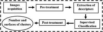
The proposed methodology is conceived to determine the affiliation of the pixels to their underlying material, whether grape or non-grape (rest of the canopy, stems, non-vine), based on the values of surrounding pixels. A pixel of interest is labelled as grape or non-grape depending on statistical descriptors extracted in a sub-window centred on it. The statistical descriptors are composed of textural and colour features. The descriptors are then submitted to a Support Vector Machine supervised classification which computes the decision function attributing the label from the descriptors. The following subparts aim at describing the data and the algorithm used for the different steps of the processing chain (Figure 1).
Processing Chain.

Image acquisition: vegetal material and instrumentation
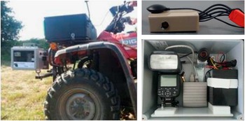
The study site is composed of two 0.5 ha plots planted respectively with Merlot (red vine) and Sauvignon blanc cultivars (white vine) in the St-Ciers-sur Gironde (Bordeaux area). During the 2015 season, 800 vine stocks were photographed in early June, prior to defoliation. At this time of the year, it is possible to observe grape bunches at different stages described by Lorenz et al. (Reference Lorenz, Eichhorn, Bleiholder, Klose, Meier and Weber1995) on the BBCH phenological scale. The bunches range from inflorescences prior to flowering (BBCH 55–57) to ‘groat-sized’ berries for the latest stages (BBCH 73). The Merlot plot has more of the stage BBCH 55–57 whereas the Sauvignon plot tends more of the stages BBCH 73. Images were taken with a device embedded on a farm quad driven between rows with an average speed of 5 km.h−1 at 70 cm from the target (Figure 2.). The device is composed of a 2 Mpx industrial RGB camera, a flash, a 12 V battery and an industrial computer, all placed in a compact and watertight plastic case. The device is completed with a GNSS receiver (G-star IV) for georeferencing and an ultrasonic sensor which provides the distance between the camera and the vine, allowing assessment of pixel size. Each image covers an area including a full vine stock and its canopy with a resolution of 1536*1200 pixels, with a square millimetre being covered by approximately 4 pixels.
Installation of the embedded device on the farm quad (left), device used for on-board acquisition (right).

Pre-processing
In order to narrow the areas where the descriptors are calculated to those which most likely contain grapes, a two-step pre-segmentation is performed. The first step consists in a thresholding in the HSV colour representation which aims at removing non-foliage areas such as the sky, ground, wood stems and trellising wires. The second step consists in thresholding based on local amplitudes of intensity gradients, extracted using a Gaussian derivative filter. These steps are meant to discard the less contrasted area such as the core of leafs and apply texture analysis only on more complex areas.
Extraction of descriptors
The textural features are composed of five Haralick’s features (Haralick, Reference Haralick1979): energy, entropy, contrast, inertia, and inverse difference moment. These features are themselves computed from Grey Level Co-occurrence Matrices (GLCM). In this study, four orientated GLCMs were computed for angles of 0°, 45°, 90° and 135°. Orientations and features are selected on the basis of a preliminary statistical study which provided the most discriminating settings. Colorimetric features, namely the means and standard deviations of the three RGB channels, are computed on the same sub-window as the Haralick’s features.
In addition, two other texture descriptors are computed from the eigenvalues λ1 and λ2 of the local structure tensor (Rosu et al., Reference Rosu, Donias, Bombrun, Said, Regniers and Da Costa2015), itself computed from the local gradients. The two extra features are the local anisotropy and energy, respectively represented by α and ε, computed with the following formula:
 $$\alpha \,{\equals}\,{{\lambda 1{\minus}\lambda 2} \over {\lambda 1{\plus}\lambda 2}},\,\alpha \in[0,1]\!;\,{\epsilon}\,{\equals}\,\lambda 1{\plus}\lambda 2$$
Supervised classifier
28 descriptors are computed for every pixel pre-selected by the pre-treatment steps. These descriptors are used as inputs for the supervised classifier. In this study, the Support Vector Machine (SVM) developed by Chang et al. (Reference Chang, Hsu and Lin2000) and available from LibSVM was chosen. A two-class classifier with Gaussian kernel (RBF: Radial Basis Function) was trained on a set of randomly chosen ground-truth images (the training set) and tested on a second set of images (the validation set). The labels ‘bunch’ and ‘non-bunch’ given as outputs of the SVM are used to create classification maps, which are the superposition of the original image and binary mask formed from the labels.
Post-processing
In order to eliminate sporadic misclassifications and fill in the potential gaps within the detected clusters, morphological operations (hole filling, erosions and dilations) and operations on connected components (thresholding regarding respective areas) are applied on the classification maps.
Results
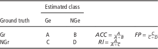
In order to evaluate the performance of the processing chain, different sets of a dozen labelled images are used as ground-truth for the learning phase. The decision function resulting from the learning phase is tested on 60 remaining images. After post treatment, three indices represent the performances: accuracy (ACC), reliability (Rl) and false positives rate (FP). Let Gr, Ge, NGr and NGe be respectively the real and estimated classes for bunches and non-bunches. The total amount of pixels belonging in the cluster class and estimated as such is A and the total amount of pixels belonging in the non-cluster class and estimated as such are D, B and C and represent then the amount of misclassified pixels for each class.
-
- ACC represent the proportion of real cluster pixels classified as such (see able 1).
-
- Rl represent the proportion of cluster pixels classified as such regarding the total number of pixels estimated as bunches (see Table 1).
-
- FP represent the proportion of non-cluster pixels misclassified in the cluster class regarding the total number of pixels belonging to non- bunches according to ground-truth (see table 1).
Definition of the confusion matric and of the performance indexes

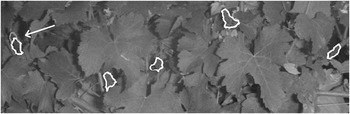
Figure 3 shows an example of classification results obtained with training set 1. Groups of adjacent pixels retained as cluster pixels, form connected components represented by their contours drawn in white. In this example, the five bunches present are detected respectfully of their morphology. The grey contour (pointed with a white arrow) represents the contours of the missing undetected parts of a bunch.
Results of automated detection of groat-sized bunches of grapes (Sauvignon blanc cultivar).

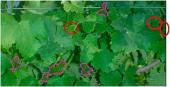
Figure 4 shows another example from set 1 where three clusters, circled in white, are undetected by the processing chain. It can be noticed that this portions belong to clusters largely occulted by the foliage. Furthermore, these undetected areas are located in a deeper and then less contrasted plan of the image
Automated detection with undetected bunches of grapes in the deep plan of the image.

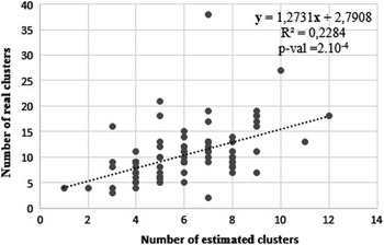
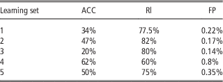
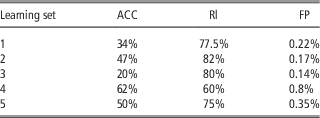
Table 2 summarizes the results of the comparison between our output and the ground truth, pixel by pixel, for five different learning sets. The reliability obtained, which is superior to 75% in average, meaning that the objects detected by the process are mostly genuine grapes which is corroborate by the false positives rate inferior to 1%. The proportion of grape surfaces detected is just under 50% on average (ACC), however, the measured surfaces are correlated to the real surfaces on ground-truth (see Figure 5) which makes it possible to estimate the real surfaces thanks to the promising truthfulness of the detection given by Rl.
Correlation between estimations and ground-truth on training set 1.

Summary of the performances of the method
Discussion
The developed processing chain achieves a detection of most of the grape bunches present on the images with a strong reliability above 75% on average. The morphology of large and average size bunches is almost fully recovered. However, when it comes to small portions of cluster largely occulted by the foliage, the process might not recover the full visible portion. Another difficulty is faced concerning the separation of agglomerated bunches which are confounded into one big cluster. Images with very few, small and scattered bunches, which are typically images with gaps in foliage or with very dense canopy, can produce sizeable false detections. The major difficulty encountered by the processing chain is the difference of contrast between objects located in different plan of depths. As a matter of fact, the bunches which are not located in the depth of field of the camera are less contrasted, their texture is then closer to some mixed regions of the foliage. For these reasons, such objects are less likely to be detected.
Conclusions
We have demonstrated that an embedded colour imaging system can provide promising measurements of grape bunches just after flowering which are correlated to ground truth. The new approach we developed is able to overcome the major difficulties encountered by shape and colour based algorithms at early stages thanks to the inclusion of more specific features from texture analysis. Even though accurate and early estimation of vine yields are not achieved yet, relative maps of fruitfulness and cropping loads can be provided. Further improvement should include a better control and management of the depth of field in order to detect bunches of grapes located deeper in the images. A validation and generalisation of the results should be the next step of development with manual measurements completed for different years and different vineyards.