2. Numerical method

2.1. Governing equations and simulation parameters

The continuity and Navier–Stokes equations for incompressible flow of two immiscible fluids with matching densities but different viscosities are

(2.1) $$\begin{eqnarray}\displaystyle & \displaystyle \frac{\partial u_{j}}{\partial x_{j}}=0, & \displaystyle\end{eqnarray}$$

(2.2) $$\begin{eqnarray}\displaystyle & \displaystyle \frac{\partial u_{i}}{\partial t}+\frac{\partial u_{i}u_{j}}{\partial x_{j}}=-\frac{\partial p}{\partial x_{i}}+\frac{1}{\mathit{Re}_{{\it\delta}_{0}}}\frac{\partial }{\partial x_{j}}\left[{\it\mu}\left(\frac{\partial u_{i}}{\partial x_{j}}+\frac{\partial u_{j}}{\partial x_{i}}\right)\right]. & \displaystyle\end{eqnarray}$$

Terms in the above equations are non-dimensionalized using the free-stream velocity $U_{\infty }$ and the single-fluid boundary-layer thickness at the inlet ${\it\delta}_{0}$ . The viscosity, ${\it\mu}$ , is normalized by its value in the top fluid. The ratio of the bottom to the top fluid viscosity is denoted ${\it\mu}_{BT}$ . The Reynolds number in the equations is defined as $\mathit{Re}_{{\it\delta}_{0}}(\equiv {\it\rho}U_{\infty }{\it\delta}_{0}/{\it\mu}_{T})=800$ . The velocity components in the streamwise ( $x$ ), wall-normal ( $y$ ) and spanwise ( $z$ ) directions are $u$ , $v$ and $w$ , respectively, and the pressure is $p$ . Hereafter, uppercase symbols refer to mean quantities, and primed symbols, such as $u^{\prime }$ , are reserved for fluctuations.

The Navier–Stokes equations were solved on a staggered grid with a local-volume-flux formulation (Rosenfeld, Kwak & Vinokur Reference Rosenfeld, Kwak and Vinokur1991). The viscous terms were integrated in time implicitly using Crank–Nicolson method and the convective terms were treated explicitly using Adams–Bashforth scheme. The overall accuracy of the present numerical method is second order in space and time. By applying the fractional step algorithm to the continuity and Navier–Stokes equations, a three-step time-advancement scheme is obtained,

(2.3) $$\begin{eqnarray}\displaystyle & \displaystyle \frac{\hat{u} _{i}-{u_{i}}^{n}}{{\rm\Delta}t}=\frac{-1}{2}(3{N_{i}}^{n}-{N_{i}}^{n-1})+\frac{1}{2}\frac{1}{\mathit{Re}_{{\it\delta}_{0}}}\frac{\partial }{\partial x_{j}}\left[{\it\mu}\frac{\partial }{\partial x_{j}}\left(\hat{u} _{i}+{u_{i}}^{n}\right)\right]-\frac{\partial {\it\Phi}^{n}}{\partial x_{i}}, & \displaystyle\end{eqnarray}$$

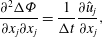(2.4) $$\begin{eqnarray}\displaystyle & \displaystyle \frac{\partial ^{2}{\rm\Delta}{\it\Phi}}{\partial x_{j}\partial x_{j}}=\frac{1}{{\rm\Delta}t}\frac{\partial \hat{u} _{j}}{\partial x_{j}}, & \displaystyle\end{eqnarray}$$

(2.5) $$\begin{eqnarray}\displaystyle & \displaystyle \frac{{u_{i}}^{n+1}-\hat{u} _{i}}{{\rm\Delta}t}=-\frac{\partial {\rm\Delta}{\it\Phi}}{\partial x_{i}}, & \displaystyle\end{eqnarray}$$

where $N$ is the discrete form of the advection term, and ${\rm\Delta}t$ is the computational time step. Here, ${\it\Phi}$ and ${\rm\Delta}{\it\Phi}$ are the pseudo-pressure and its time difference ( ${\it\Phi}^{n+1}-{\it\Phi}^{n}$ ), respectively. By adopting the ${\rm\Delta}{\it\Phi}$ form of the discrete Navier–Stokes equations, we enforce the appropriate boundary conditions on the velocity field directly without the need to incorporate the pressure gradient term (Kim & Moin Reference Kim and Moin1985).

In general, the solution to the pressure equation is computationally expensive due to the elliptic nature of the problem, and this issue is exacerbated in the case of variable fluid properties (van der Vorst Reference van der Vorst2003). For example, in the general two-fluid case where the density varies across the interface, we solve the Poisson equation using biconjugate gradient stabilized (BiCGStab) method (van der Vorst Reference van der Vorst1992) with a three-dimensional multigrid preconditioner. The Krylov-based method is advantageous for fast convergence of the solution in the presence of the jump in shear across the two-fluid interface. In the matched density case which we consider here, a significant computational advantage is achieved by applying a Fourier transform in the span and converting the pressure Poisson equation into a Helmholtz equation.

The convective outflow condition $\partial u/\partial t+c\partial u/\partial x=0$ was applied at the outlet where $c$ is the local bulk velocity. The no-slip condition was imposed at the bottom wall. The top boundary conditions were $\partial u/\partial y=\partial w/\partial y=0$ and $v=-\!\int \!\partial u/\partial x\,\text{d}y$ . Periodic boundary conditions were applied in the spanwise direction.

Two free-stream turbulence intensities were simulated, $\mathit{Tu}=2.5\,\%$ and $3.5\,\%$ . The sizes of the computational domains and the number of grid points are provided in table 1. The computational domain is a rectangular box with a sufficiently large spanwise extent in order to avoid spurious correlations. For the lower turbulence intensity case, the length of computational domain is longer, $2.6\times 10^{4}<\,\mathit{Re}_{x}(\equiv {\it\rho}U_{\infty }x/{\it\mu}_{T})<\,9.9\times 10^{5}$ , in order to capture the full transition process. The grid is clustered in the wall-normal direction, and is uniformly distributed in the streamwise and spanwise directions. Table 1 also reports the grid resolution and the computational time step in wall units scaled using the maximum friction velocity, $\max _{x}u_{{\it\tau}}(x)$ , from the single-fluid computation which provides a conservative estimate. The computational time step was 0.01 ${\it\delta}_{0}/U_{\infty }$ . Beyond the initial transient, the total averaging time was 2400 ${\it\delta}_{0}/U_{\infty }$ time units. Simulations of the two-fluid boundary layers are particularly challenging due the computational requirements associated with tracking the interface as discussed below.

Table 1.

Summary of simulation parameters, and the spatial and temporal resolutions.

2.2. Level set method

The level set method introduced by Osher & Sethian (Reference Osher and Sethian1988) has been widely used in simulations of multiphase flows. This method is based on an implicit representation of the interface for which the equation of motion is

(2.6) $$\begin{eqnarray}\frac{\partial {\it\phi}}{\partial t}+\frac{\partial u_{j}{\it\phi}}{\partial x_{j}}=0,\end{eqnarray}$$

where ${\it\phi}$ is the level set function. In the conventional level set technique, a signed distance function depicting the interface as ${\it\phi}=0$ is used. Advantages of the level set method include automatic handling of topological changes, efficient parallelization as well as simplicity of evaluating geometric quantities. However, one of the main limitations of this method is poor mass conservation. In order to overcome this difficulty, we adopted the conservative level set method proposed by Desjardins, Moureau & Pitsch (Reference Desjardins, Moureau and Pitsch2008). This method ensures accurate and robust interface transport by using a hyperbolic tangent function,

(2.7) $$\begin{eqnarray}{\it\psi}=\frac{1}{2}\left(\tanh \left(\frac{{\it\phi}}{2{\it\epsilon}}\right)+1\right),\end{eqnarray}$$

where ${\it\epsilon}\equiv 0.5\min ({\rm\Delta}x,{\rm\Delta}y,{\rm\Delta}z)$ is a parameter which sets the thickness of the interface. The interface location is now portrayed by the iso-surface ${\it\psi}=0.5$ . The transport equation for ${\it\psi}$ corresponding to the advection of the interface is

(2.8) $$\begin{eqnarray}\frac{\partial {\it\psi}}{\partial t}+\frac{\partial u_{j}{\it\psi}}{\partial x_{j}}=0.\end{eqnarray}$$

Due to the sharp change in ${\it\psi}$ across the interface, the above equation accurately approximates the material derivative of fluid properties, such as $\text{D}{\it\mu}/\text{D}t=0$ .

In the presence of sharp gradients of velocity and pressure across the interface, it is computationally very challenging to maintain ${\it\psi}$ as a non-oscillatory function. Distorted ${\it\psi}$ incurs unphysical oscillations. The difficulty is attributed to the nature of the Hamilton–Jacobi-type equation (2.8) (Sethian & Smereka Reference Sethian and Smereka2003). In order to maintain the smoothness of ${\it\psi}$ , we introduced the re-initialization equation,

(2.9) $$\begin{eqnarray}\frac{\partial {\it\psi}}{\partial {\it\tau}}+\boldsymbol{{\rm\nabla}}\boldsymbol{\cdot }({\it\psi}(1-{\it\psi})\boldsymbol{n})=\boldsymbol{{\rm\nabla}}\boldsymbol{\cdot }({\it\epsilon}(\boldsymbol{{\rm\nabla}}{\it\psi}\boldsymbol{\cdot }\boldsymbol{n})\boldsymbol{n}),\end{eqnarray}$$

where ${\it\tau}$ and $\boldsymbol{n}\equiv \boldsymbol{{\rm\nabla}}{\it\psi}/|\boldsymbol{{\rm\nabla}}{\it\psi}|$ are the pseudo-time step and the interface normal vector, respectively. The above equation is composed of a compression term on the left-hand side which sharpens the interface, and a diffusion term on the right-hand side which maintains numerical stability. Solution of (2.9) is repeated until the steady state is reached. Typically, three or four iterations were required for the convergence of the solution by setting ${\rm\Delta}{\it\tau}={\it\epsilon}$ . The physical properties of the two fluids are computed from

(2.10) $$\begin{eqnarray}{\it\mu}={\it\mu}_{BT}+(1-{\it\mu}_{BT}){\it\psi}.\end{eqnarray}$$

The third-order total variation diminishing (TVD) Runge–Kutta scheme (Shu & Osher Reference Shu and Osher1988) was used for time integration of (2.8) and (2.9). To accurately resolve the sharp interface profile, a fifth-order upstream central scheme (Nourgaliev & Theofanous Reference Nourgaliev and Theofanous2007) was employed for the convective term of (2.8). The compression and diffusion terms in (2.9) were spatially discretized by second-order central differencing.

The computations of (2.8) and (2.9) for the entire domain are inefficient owing to the interface movement within a confined region. In order to reduce the computational effort, an adaptive narrow-band approach was exploited (Peng et al. Reference Peng, Merriman, Osher, Zhao and Kang1999). In this method, a narrow band formed by a few grid cells around the interface is introduced using a mask function. The mask function identifies the grid points within the narrow band and then the level-set and re-initialization equations are solved at these points. In addition, a multilevel mesh refinement (MMR) for the level-set function was utilized to improve the spatial resolution of the interface transport. In this approach, the flow field is solved at the coarsest mesh and the level-set function is evaluated at the finest grid. The multigrid hierarchy with three levels was selected in the $x$ and $z$ directions. There was no additional multilevel grid refinement in the $y$ direction.

The present level-set algorithm has been validated extensively by comparison to linear and nonlinear stability results (see Cheung & Zaki Reference Cheung and Zaki2011). In addition, two canonical interface tracking problems were also examined: the transport of Zalesak’s disk (Zalesak Reference Zalesak1979) and the rise of an air bubble in quiescent water (Gueyffier et al. Reference Gueyffier, Li, Nadim, Scardovelli and Zaleski1999; Yang & Stern Reference Yang and Stern2009). In the case of the Zalesak’s disk, the size of the computational domain was $(L_{x},L_{y})=(100,100)$ and the number of grid points was $(N_{x},N_{y})=(257,257)$ . Solid-body rotation, $u=({\rm\pi}/314)(50-y)$ and $v=({\rm\pi}/314)(x-50)$ , was prescribed to the disk for 10 revolutions and the error in the interface location was evaluated using the $L_{1}$ -norm,

(2.11) $$\begin{eqnarray}{\it\varepsilon}\equiv \frac{1}{L}\int |H({\it\psi}_{exact})-H({\it\psi}_{computed})|\,\text{d}x\,\text{d}y,\end{eqnarray}$$

where $L$ is the perimeter of the expected interface and the indicator function $H=\{0,1\}$ distinguishes the inner and outer regions of the disk. After 1, 2, 5 and 10 full rotations, the errors were ${\it\varepsilon}=0.028$ , 0.032, 0.042 and 0.062, respectively. For the rising bubble, the size of the computational domain was $(L_{x},L_{y},L_{z})=(12,24,12)R$ where $R$ is the radius of the initially spherical bubble. The number of grid points in each direction was $(N_{x},N_{y},N_{z})=(129,257,129)$ . The viscosity and density ratios of air to water were prescribed, ${\it\mu}_{a}/{\it\mu}_{w}=0.085$ and ${\it\rho}_{a}/{\it\rho}_{w}=0.0011$ , and the terminal velocity was chosen as the reference scale. The Reynolds, Froude and Weber numbers were $\mathit{Re}=9.8$ , $\mathit{Fr}=0.8718$ and $\mathit{We}=7.6$ . The bubble was released at an initial position $(x/R,y/R)=(6.0,1.5)$ . As the bubble rose, its deformation, vertical displacement and rising speed agreed with the results by Gueyffier et al. (Reference Gueyffier, Li, Nadim, Scardovelli and Zaleski1999) and Yang & Stern (Reference Yang and Stern2009).

2.3. Inflow generation

The base flow at the inlet to the computational domain is a two-fluid boundary layer $\boldsymbol{U}=[U_{j}(y),V_{j}(y),0]$ with density ${\it\rho}$ and dynamic viscosities ${\it\mu}_{j}$ . The subscript $j=\{T,B\}$ denotes the top and bottom fluids, respectively. The base flow is obtained by solving the following equation in boundary-layer coordinates (Nelson, Alving & Joseph Reference Nelson, Alving and Joseph1995),

(2.12) $$\begin{eqnarray}F\frac{\partial ^{2}F}{\partial {\it\zeta}^{2}}+{\it\nu}_{j}\frac{\partial ^{3}F}{\partial {\it\zeta}^{3}}-{\it\chi}\left(\frac{\partial F}{\partial {\it\zeta}}\frac{\partial }{\partial {\it\chi}}\left(\frac{\partial F}{\partial {\it\zeta}}\right)-\frac{\partial ^{2}F}{\partial {\it\zeta}^{2}}\frac{\partial F}{\partial {\it\chi}}\right)=0\end{eqnarray}$$

where ${\it\nu}_{j}={\it\mu}_{j}/{\it\rho}$ , ${\it\chi}\equiv \sqrt{U_{\infty }x/(2{\it\nu}_{T})}$ , ${\it\zeta}\equiv y\sqrt{U_{\infty }/(2{\it\nu}_{T}x)}$ and $F\equiv {\it\Psi}/\sqrt{2{\it\nu}_{T}U_{\infty }x}$ . Here, ${\it\Psi}$ and $x$ are the streamfunction and the downstream location from the leading edge, respectively. The interface height ${\it\zeta}^{\ast }$ is governed by the kinematic condition:

(2.13) $$\begin{eqnarray}\frac{\partial {\it\zeta}^{\ast }}{\partial {\it\chi}}=\frac{1}{{\it\chi}}\left(\frac{V^{\ast }}{U^{\ast }}-{\it\zeta}^{\ast }\right)\end{eqnarray}$$

where $U^{\ast }$ and $V^{\ast }$ are the mean streamwise and wall-normal velocities at the interface. The wall $(y=0)$ and free-stream $(y\rightarrow \infty )$ boundary conditions on $F$ are

(2.14a−c ) $$\begin{eqnarray}F_{B}(0)=0;\quad \frac{\text{d}F_{B}}{\text{d}{\it\zeta}}(0)=0;\quad \frac{\text{d}F_{T}}{\text{d}{\it\zeta}}(y\rightarrow \infty )=1.\end{eqnarray}$$

In addition, at the interface location, ${\it\zeta}={\it\zeta}^{\ast }$ , the following velocity and stress continuity conditions must be satisfied,

(2.15a−c ) $$\begin{eqnarray}F_{B}=F_{T};\quad \frac{\text{d}F_{B}}{\text{d}{\it\zeta}}=\frac{\text{d}F_{T}}{\text{d}{\it\zeta}};\quad {\it\mu}_{B}\frac{\text{d}^{2}F_{B}}{\text{d}{\it\zeta}^{2}}={\it\mu}_{T}\frac{\text{d}^{2}F_{T}}{\text{d}{\it\zeta}^{2}}.\end{eqnarray}$$

Equations (2.12)–(2.15) do not admit a similarity solution. Therefore, obtaining a mean-velocity profile to apply as an inflow condition in the DNS requires marching the above equations from an upstream location up to the DNS inflow plane, $x_{0}$ . Two additional requirements are imposed: (i) all of the two-fluid DNSs must start at the same distance $x_{0}$ from the leading edge; and (ii) the film thickness must be 10 % at that location. Since both the boundary layer and the film spread at different rates, an iterative procedure is required to satisfy these requirements. Equations (2.12)–(2.15) are solved starting upstream of $x_{0}$ with a guess of the film thickness at that location (the guess is larger than 10 % relative to the local boundary-layer thickness since the film spreading rate is slower than the outer flow). The solution is marched downstream up to the inlet of the DNS domain, and the film thickness is verified at $x_{0}$ . This procedure is iterated to convergence, and ensures that the inflow profiles for the single- and two-fluid DNSs are solutions to the boundary-layer equations, start at the same distance to the leading edge, and have the desired film thickness.

In order to prescribe realistic free-stream vortical disturbances, isotropic turbulence was synthesized at the inlet. Following the work by Jacobs & Durbin (Reference Jacobs and Durbin2001), the disturbances are expressed in terms of Fourier modes in the spanwise dimension and in time, and a superposition of Orr–Sommerfeld (OS) and Squire eigenfunctions in the wall-normal direction. The eigenfunctions are solutions to the homogeneous OS and Squire equations for the two-fluid boundary layer. The free-stream turbulence satisfies the von Kármán spectrum

(2.16) $$\begin{eqnarray}E({\it\kappa})=\mathit{Tu}^{2}\frac{L^{5}{\it\kappa}^{4}}{C[1+({\it\kappa}L)^{2}]^{17/6}},\end{eqnarray}$$

where $C=0.688$ , and ${\it\kappa}\equiv \sqrt{{\it\omega}^{2}+k_{y}^{2}+k_{z}^{2}}$ and $L$ are the wavenumber and turbulence length scale, respectively. Here, the wall-normal and spanwise wavenumbers are denoted $k_{y}$ and $k_{z}$ , respectively, and ${\it\omega}$ is the frequency of the perturbation. Note that $L\equiv (55C/9{\rm\pi})L_{11}$ and $L_{11}=\int _{0}^{\infty }\overline{u^{\prime }(x)u^{\prime }(x+r)}\,\text{d}r/\mathit{Tu}^{2}$ . The turbulence intensity, $\mathit{Tu}$ , is given by

(2.17) $$\begin{eqnarray}\mathit{Tu}=\sqrt{\frac{2}{3}\int _{0}^{\infty }E({\it\kappa})\,\text{d}{\it\kappa}}.\end{eqnarray}$$

Two turbulence intensities ( $\mathit{Tu}=2.5\,\%$ and $3.5\,\%$ ) were examined in the present study. In the case with $\mathit{Tu}=2.5\,\%$ , the initial turbulence intensity decays to $0.2\,\%$ near the exit of the simulation domain as shown in figure 2. The decay rate of the turbulence intensity has the form, $\mathit{Tu}\propto (x-x_{g})^{-n}$ where $x_{g}$ is the virtual origin of the grid turbulence and $n\simeq 0.8$ . This exponent is consistent with the experimental results by Kurian & Fransson (Reference Kurian and Fransson2009), where $\mathit{Tu}^{2}$ is shown to decay according to an exponential rate in the range, $-1.6<2n<-1.2$ .

Figure 2.

Streamwise decay of the free-stream turbulence intensity. At the inlet, $\mathit{Tu}=2.5\,\%$ .

3. Reynolds-averaged statistics

In this section, various statistical measures related to bypass transition in two-fluid boundary layers are presented, and the discussion is focused on the lower turbulence intensity simulations ( $\mathit{Tu}=2.5\,\%$ ). The mechanism underlying the observed trends is further analysed in § 4 by examining instantaneous and conditionally sampled flow fields. Finally, § 5 reports on the efficacy of the wall film in the case of higher $\mathit{Tu}$ .

In order to provide clear evidence of transition delay in the two-fluid configuration, the skin-friction coefficient, $C_{f}$ , is reported in figure 3. Transition to turbulence causes a substantial increase in $C_{f}$ , and it is evident from figure 3 that a less-viscous wall-film suppresses the onset of transition. The skin friction curve departs significantly from the Blasius value ( $C_{f}=0.664/\sqrt{\mathit{Re }_{x}}$ ) starting at $x-x_{0}\approx 400$ , 500 and 750 when ${\it\mu}_{BT}=1.0$ , 0.5 and 0.2, respectively. The completion of transition is herein defined as the point where $C_{f}$ attains its maximum near the turbulent correlation ( $C_{f}=0.455/[\ln (0.06\mathit{Re}_{x})]^{2}$ ). Transition is complete at $x-x_{0}\approx 1100$ and 1000 for ${\it\mu}_{BT}=1.0$ and 0.5, respectively. In the case of ${\it\mu}_{BT}=0.2$ , the fully turbulent state is not reached within the computational domain.

Figure 3.

Downstream evolution of the skin friction coefficient for $\mathit{Tu}=2.5\,\%$ .

A slightly more detailed view of the changes to $C_{f}$ in the case of transition delay is sought. A modification of the identity by Fukagata, Iwamoto & Kasagi (Reference Fukagata, Iwamoto and Kasagi2002), referred to hereafter as FIK, is adopted. The FIK identity is computed from the triple integration of the Reynolds-averaged Navier–Stokes (RANS) equations for the streamwise momentum in the wall normal direction, and it can provide a detailed view of the various contributions to $C_{f}$ . For the present flow, the FIK identity is modified to take into account the viscosity distribution,

(3.1) $$\begin{eqnarray}\displaystyle C_{f,FIK} & = & \displaystyle \underbrace{\frac{4}{{\it\delta}_{99}^{2}\mathit{Re}_{{\it\delta}_{0}}}\int _{0}^{{\it\delta}_{99}}\overline{{\it\nu}}U\,\text{d}y}_{\mathit{FIK}_{lam}}-\underbrace{\frac{4}{{\it\delta}_{99}^{2}}\int _{0}^{{\it\delta}_{99}}({\it\delta}_{99}-y)\overline{u^{\prime }v^{\prime }}\,\text{d}y}_{\mathit{FIK}_{\overline{u^{\prime }v^{\prime }}}}\nonumber\\ \displaystyle & & \displaystyle +\,\underbrace{\frac{4}{{\it\delta}_{99}^{2}\mathit{Re}_{{\it\delta}_{0}}}\int _{0}^{{\it\delta}_{99}}({\it\delta}_{99}-y)\left(-U\frac{\partial \overline{{\it\nu}}}{\partial y}+\overline{{\it\nu}^{\prime }\frac{\partial u^{\prime }}{\partial y}}\right)\,\text{d}y}_{\mathit{FIK}_{vis}}-\frac{4}{{\it\delta}_{99}^{2}}\int _{0}^{{\it\delta}_{99}}({\it\delta}_{99}-y)UV\,\text{d}y\nonumber\\ \displaystyle & & \displaystyle -\,\frac{2}{{\it\delta}_{99}^{2}}\int _{0}^{{\it\delta}_{99}}({\it\delta}_{99}-y)^{2}\left[\frac{\partial }{\partial x}(UU)+\frac{\partial }{\partial x}(\overline{u^{\prime }u^{\prime }})\right]\,\text{d}y\nonumber\\ \displaystyle & & \displaystyle +\,\frac{2}{{\it\delta}_{99}^{2}\mathit{Re}_{{\it\delta}_{0}}}\int _{0}^{{\it\delta}_{99}}({\it\delta}_{99}-y)^{2}\left[\frac{\partial }{\partial x}\left(\overline{{\it\nu}}\frac{\partial U}{\partial x}\right)+\frac{\partial }{\partial x}\left(\overline{{\it\nu}^{\prime }\frac{\partial u^{\prime }}{\partial x}}\right)\right]\,\text{d}y\nonumber\\ \displaystyle & & \displaystyle +\,\frac{2}{{\it\delta}_{99}^{2}}\int _{0}^{{\it\delta}_{99}}({\it\delta}_{99}-y)^{2}\left(-\frac{\partial P}{\partial x}\right)\,\text{d}y.\end{eqnarray}$$

Here, $\mathit{FIK}_{lam}$ , $\mathit{FIK}_{\overline{u^{\prime }v^{\prime }}}$ , $\mathit{FIK}_{vis}$ denote the contributions of the laminar base flow, Reynolds shear stress and viscosity variation in the $y$ direction, respectively. Note that the overbar represents time-averaged quantities. In (3.1), $C_{f}$ is decomposed into the effects of mean and fluctuating motion as well as the variable local viscosity. In general, skin friction is related to the near-wall turbulence structures (Kravchenko, Choi & Moin Reference Kravchenko, Choi and Moin1993; Choi, Moin & Kim Reference Choi, Moin and Kim1994). This formulation demonstrates the higher impact of near-wall turbulence motions as dictated by the moments in the integrals.

Figure 4 displays contributions of the first three terms of (3.1) to the skin-friction coefficient for ${\it\mu}_{BT}=1.0$ and 0.2. The sum of the remaining terms is also included and is denoted $\mathit{FIK}_{other}$ . The skin-friction coefficient obtained from the FIK identity ( $C_{f,FIK}$ ) is in good agreement with the time-averaged $C_{f}$ evaluated during the DNS.

Figure 4.

Contributions to the Skin friction coefficients for (a) ${\it\mu}_{BT}=1.0$ and (b) ${\it\mu}_{BT}=0.2$ .

In the pretransitional boundary layer, the total $C_{f}$ shadows the laminar curve, with an offset due to the energetic streak distortions. While the streaks have a significant $\overline{u^{\prime }u^{\prime }}$ contribution, they do not have an appreciable associated Reynolds shear stress. The term $\mathit{FIK}_{\overline{u^{\prime }v^{\prime }}}$ is therefore relatively small in the pretransitional regime. With the onset of transition to turbulence, energy is redistributed from $\overline{u^{\prime }u^{\prime }}$ to $\overline{u^{\prime }v^{\prime }}$ and the increase in $\mathit{FIK}_{\overline{u^{\prime }v^{\prime }}}$ is mirrored in the total $C_{f}$ curve. Relative to the single-fluid flow, the abrupt increase of $\mathit{FIK}_{\overline{u^{\prime }v^{\prime }}}$ is delayed downstream in the presence of the wall film.

The large contribution of $\mathit{FIK}_{lam}$ seen in figure 4(b) near the inlet ( $x-x_{0}<100$ ) is due to the fuller profile of the streamwise mean velocity. The change of viscosity in the wall-normal direction leads to the decrease in $C_{f}$ as demonstrated by the figure. This is mainly due to the large positive gradient of mean viscosity. Note that, unlike the instantaneous viscosity profile which is sharp, the average viscosity has a smoother profile due to the time dependence of the interface location. Nonetheless $\overline{{\it\nu}}(y)$ retains a sufficiently large $\partial \overline{{\it\nu}}/\partial y$ up to $x-x_{0}\approx 200$ .

The downstream growth of boundary-layer 99 % and momentum thicknesses are shown in figure 5(a,c). Initially ${\it\delta}_{99}$ and ${\it\theta}$ increase gradually following the Blasius solution in the laminar region, but subsequently increase at a higher rate in the transition zone. The rise in the momentum thickness reflects the sharp increase in skin friction across the transition region, and is delayed further downstream in the presence of the wall film. The downstream spreading of the wall film is shown in figure 5(b). Its growth rate is slower than that of ${\it\delta}_{99}$ and, as a result, the local ratio of the film-to-boundary-layer thickness, $d/{\it\delta}_{99}$ , decreases downstream. The film thicknesses for ${\it\mu}_{BT}=0.5$ and 0.2 are only reported up to $x-x_{0}\approx 450$ and 600, respectively. In the transition zone, the wall film is detached due to vigorous buffeting by the turbulence spots.

Figure 5.

Profiles of (a) boundary-layer 99 % thicknesses ( ${\it\delta}_{99}/{\it\delta}_{0}$ ), (b) film thicknesses ( $d/{\it\delta}_{0}$ black lines; $d/{\it\delta}_{99}$ light lines) and (c) momentum thicknesses ( ${\it\theta}/{\it\delta}_{0}$ ).

The influence of the viscosity ratio on the mean velocity at several $x$ locations is shown in figure 6. Here, the $y$ -axis is normalized by the local boundary-layer thickness ${\it\delta}_{99}$ . The purpose of introducing the wall film is achieved as the mean shear in the pretransitional regime is increasingly contained within the film at lower film viscosities. Upstream of transition, the fuller mean profile within the less-viscous film flow explains the large contribution of $\mathit{FIK}_{lam}$ to $C_{f}$ shown in figure 4(b). After the onset of transition, the mean velocity in the single-fluid boundary layer increases near the wall. However, the mean velocity for ${\it\mu}_{BT}=0.2$ retains the laminar profile up to $x-x_{0}=800$ due to transition delay. With weaker outer shear in the two-fluid flow, it is anticipated that the lift-up mechanism in the bulk fluid will be weakened, although the change in the disturbance field within the film is more difficult to anticipate.

Figure 6.

Mean velocity profiles at various downstream locations. On the $x$ -axis, the distance between major tick marks denotes $U_{x}=1.0U_{\infty }$ .

The root-mean-square (r.m.s.) of the streamwise velocity fluctuations is plotted in figure 7 for different $x$ -locations. The streamwise velocity fluctuations for ${\it\mu}_{BT}=1.0$ amplify with downstream distance. The distribution of $u_{rms}^{\prime }$ shows a maximum approximately in the middle of the laminar boundary layer ( $y/{\it\delta}_{99}\approx 0.4$ corresponding to $y/{\it\delta}^{\ast }\approx 1.2$ ), which is in agreement with previous results from experiments and numerical simulations (Matsubara & Alfredsson Reference Matsubara and Alfredsson2001; Brandt, Schlatter & Henningson Reference Brandt, Schlatter and Henningson2004). The laminar $u_{rms}^{\prime }$ profiles of ${\it\mu}_{BT}=1.0~(x-x_{0}<\,300)$ have the appearance of Klebanoff modes. After the onset of transition, the peak of the velocity fluctuation shifts towards the wall.

Figure 7.

Profiles of the r.m.s. streamwise velocity fluctuations at various downstream locations. On the $x$ -axis, the distance between major tick marks denotes $u_{rms}^{\prime }=0.17U_{\infty }$ .

The general trend of $u_{rms}^{\prime }$ described above is also observed in the two-fluid flows, although with two important changes. First, the amplitude of fluctuations becomes weaker with decreasing film viscosity. This is consistent with the linear prediction that lower-viscosity wall films attenuate the energy amplification inside the boundary layer (Saha et al. Reference Saha, Jung and Zaki2010). Second, a new peak in $u_{rms}^{\prime }$ emerges near the interface ( $y/{\it\delta}_{99}\approx 0.05$ ) in the laminar region in the case of ${\it\mu}_{BT}=0.2$ . This peak persists up to the pretransitional regime. Both observations will be quantified, and will be explained with the aid of linear theory.

The maximum value of $u_{rms}^{\prime }$ is extracted at every downstream location and is plotted in figure 8. Here, the outer peak refers to the maximum located in the middle of boundary layer and the inner peak denotes the one closer to the wall. In the single-fluid boundary layer, only one peak exists and is reproduced in both figures for reference. The amplification of the outer peak in the laminar region ( $x-x_{0}<\,200$ ) is reduced with decreasing film viscosity. This suggests that the streak amplification is weakened in two-fluid boundary layers. After transition onset, the outer peaks of ${\it\mu}_{BT}=1.0$ and 0.5 grow rapidly ( $x-x_{0}=400$ and 500) and attain maxima at $x-x_{0}=640$ and 800, respectively. It is seen in figure 8(b) that the inner peak of ${\it\mu}_{BT}=0.5$ is only discernible in the region of $x-x_{0}<\,400$ .

Figure 8.

Maximum $u_{rms}^{\prime }$ versus downstream distance for (a) outer peak and (b) inner peak. For ${\it\mu}_{BT}=0.2$ , the two peaks become indistinguishable in the region $x-x_{0}>800$ (light line).

The outer peak is weakest for ${\it\mu}_{BT}=0.2$ . In contrast to higher viscosity ratios, the inner peak has a comparable amplitude to the outer streaks when ${\it\mu}_{BT}=0.2$ . Beyond $x-x_{0}>800$ , the outer and inner peaks in $u_{rms}^{\prime }$ are indistinguishable. They increase sharply and reach a peak value at $x-x_{0}=1080$ .

In figure 9, the wall-normal locations of the maximum $u_{rms}^{\prime }$ are displayed. The laminar outer peaks lie between $0.38<\,y/{\it\delta}_{99}<\,0.5$ as shown in figure 7. It is clear that the outer peaks move rapidly towards the wall in the transition regime. In the fully turbulent regime, when ${\it\mu}_{BT}=1.0$ or 0.5, the outer peak is located at $y/{\it\delta}_{99}\approx 0.025$ . This $y$ location corresponds to $y^{+}\approx 14.5$ which is similar to the value from previous experiments (e.g. Matsubara & Alfredsson Reference Matsubara and Alfredsson2001). The inner peak for two-fluid boundary layers is placed between $0.03<\,y/{\it\delta}_{99}<\,0.1$ .

Figure 9.

Wall-normal location of maximum $u_{rms}^{\prime }$ versus downstream distance for (a) outer peak and (b) inner peak. For ${\it\mu}_{BT}=0.2$ , the outer peak moves towards the wall quickly in the transition zone, and the two peaks become indistinguishable downstream (light line).

The Reynolds-averaged streamwise velocity fluctuations reveal that the laminar streaks are weakened in two-fluid boundary layers. The origin of this trend can be explained with the aid of linear theory. The linear perturbation equations for the wall-normal velocity and vorticity are

(3.2) $$\begin{eqnarray}\frac{\partial }{\partial t}\left[\begin{array}{@{}c@{}}{\rm\nabla}^{2}v_{j}^{\prime }\\ f^{\prime }\\ {\it\eta}_{j}^{\prime }\end{array}\right]=\left[\begin{array}{@{}ccc@{}}\displaystyle \frac{\text{d}^{2}U_{j}}{\text{d}y^{2}}\frac{\partial }{\partial x}+{\it\nu}_{j}{\rm\nabla}^{4}-U_{j}\frac{\partial }{\partial x}{\rm\nabla}^{2} & 0 & 0\\ {\it\delta}(y-d) & \displaystyle -U(d)\frac{\partial }{\partial x} & 0\\ \displaystyle \frac{\text{d}U_{j}}{\text{d}y}\frac{\partial }{\partial z} & 0 & \displaystyle {\it\nu}_{j}{\rm\nabla}^{2}{\it\eta}-U_{j}\frac{\partial }{\partial x}\end{array}\right]\left[\begin{array}{@{}c@{}}v_{j}^{\prime }\\ f^{\prime }\\ {\it\eta}_{j}^{\prime }\end{array}\right]\end{eqnarray}$$

where ${\it\delta}(y-d)$ is the delta function at the interface location and $f^{\prime }$ is the interfacial displacement. These equations have appeared previously in the literature on linear stability of two-fluid flows, albeit they are often reported in Fourier space (e.g. Yih Reference Yih1967; Yecko & Zaleski Reference Yecko and Zaleski2005; Malik & Hooper Reference Malik and Hooper2007; Cheung & Zaki Reference Cheung and Zaki2010). No-slip and no-penetration boundary conditions are applied at the wall. Homogeneous boundary conditions are imposed on $v^{\prime },\partial v^{\prime }/\partial y$ and ${\it\eta}^{\prime }$ in the free stream:

(3.3a−c ) $$\begin{eqnarray}v_{B}^{\prime }(0)=0;\quad \partial _{y}v_{B}^{\prime }(0)=0;\quad {\it\eta}_{B}^{\prime }(0)=0\end{eqnarray}$$

(3.4a−c ) $$\begin{eqnarray}v_{T}^{\prime }(y\rightarrow \infty )=0;\quad \partial _{y}v_{T}^{\prime }(y\rightarrow \infty )=0;\quad {\it\eta}_{T}^{\prime }(y\rightarrow \infty )=0.\end{eqnarray}$$

In addition, the perturbation field must satisfy continuity of velocity and stresses linearized to the mean interface location, which can be expressed in terms of $v$  and  ${\it\eta}$ ,

(3.5a ) $$\begin{eqnarray}\displaystyle & [v^{\prime }]=0; & \displaystyle\end{eqnarray}$$

(3.5b ) $$\begin{eqnarray}\displaystyle & \displaystyle \left[\frac{\partial v^{\prime }}{\partial y}\right]=\left[\frac{\text{d}U}{\text{d}y}\right]\frac{\partial f^{\prime }}{\partial x}; & \displaystyle\end{eqnarray}$$

(3.5c ) $$\begin{eqnarray}\displaystyle & \displaystyle \left[{\it\mu}\left(\frac{\partial ^{2}v^{\prime }}{\partial y^{2}}-{\rm\nabla}_{xz}^{2}v^{\prime }\right)\right]=\left[{\it\mu}\frac{\text{d}^{2}U}{\text{d}y^{2}}\right]\frac{\partial f^{\prime }}{\partial x}; & \displaystyle\end{eqnarray}$$

(3.5d ) $$\begin{eqnarray}\displaystyle & \displaystyle \left[{\it\rho}\left(\frac{\partial }{\partial t}\frac{\partial v^{\prime }}{\partial y}+U\frac{\partial ^{2}v^{\prime }}{\partial x\partial y}-\frac{\text{d}U}{\text{d}y}\frac{\partial v^{\prime }}{\partial x}\right)-{\it\mu}\frac{\partial ^{3}v^{\prime }}{\partial y^{3}}-3{\it\mu}{\rm\nabla}_{xz}^{2}\frac{\partial v^{\prime }}{\partial y}\right]={\it\sigma}{\rm\nabla}_{xz}^{4}f^{\prime }; & \displaystyle\end{eqnarray}$$

(3.5e ) $$\begin{eqnarray}\displaystyle & \displaystyle [{\it\eta}^{\prime }]=-\left[\frac{\text{d}U}{\text{d}y}\right]\frac{\partial f^{\prime }}{\partial z}; & \displaystyle\end{eqnarray}$$

(3.5f ) $$\begin{eqnarray}\displaystyle & \displaystyle \left[{\it\mu}\frac{\partial {\it\eta}^{\prime }}{\partial y}\right]=-\left[{\it\mu}\frac{\text{d}^{2}U}{\text{d}y^{2}}\right]\frac{\partial f^{\prime }}{\partial z} & \displaystyle\end{eqnarray}$$

${\rm\nabla}_{xz}^{2}$

$x{-}z$

$[\cdot ]$

$(\cdot )_{T}-(\cdot )_{B}$

${\it\sigma}$

As seen in (3.2), wall-normal vorticity can be generated by tilting of the mean spanwise vorticity. In the limit of streamwise-elongated disturbances, the amplification of ${\it\eta}^{\prime }$ is representative of the behaviour of $u^{\prime }$ , or the streaks, since ${\it\eta}^{\prime }=\partial u^{\prime }/\partial z-\partial w^{\prime }/\partial x$ . Figure 10 shows the quantity $v_{rms}^{\prime }\,\text{d}U/\text{d}y$ , which is closely related to the forcing term of ${\it\eta}^{\prime }$ in (3.2), at four different $x$ positions. In general, this term decays downstream in the laminar-flow regime due to the decay of $v_{rms}^{\prime }$ . However, the profiles show a clear variability with viscosity ratio. In the single-fluid case, the profile has only one peak, while the two-fluid cases have two peaks: an outer one which is located at $y/{\it\delta}_{99}\approx 0.55$ and an inner one at $y/{\it\delta}_{99}=0.1$ . The magnitude of the outer peak diminishes with decreasing ${\it\mu}_{BT}$ since the wall film absorbs the mean shear which becomes weaker in the outer fluid (see figure 6). This weakening of the vorticity tilting term in the top fluid explains the weaker Klebanoff streaks in figure 7. On the other hand, the inner peak is intensified with the reduction in viscosity ratio (see figure 10 a). This can lead to stronger ${\it\eta}^{\prime }$ , and therefore streaks, near the interface. At the interface itself, this effect is captured by the matching condition (3.5e ), where the jump in mean shear can become a source of ${\it\eta}^{\prime }$ if the interface is deformed. The response is the inner peak in $u_{rms}^{\prime }$ reported in figure 8(b), which is enhanced as ${\it\mu}_{BT}$ is reduced.

Figure 10.

Profiles of $v_{rms}^{\prime }\,\text{d}U/\text{d}y$ for (a) $x-x_{0}=50$ , (b) $x-x_{0}=100$ , (c) $x-x_{0}=150$ and (d) $x-x_{0}=200$ .

Linear theory provides a viable starting point to explain the changes in the $u$ -perturbation field in the nonlinear simulations. In the context of the DNS, the relevant term is $\overline{u^{\prime }v^{\prime }}(\partial U/\partial y)$ , or production due to the Reynolds’ shear stress. This term is analysed in detail below. It is also important to note that weaker $u_{rms}^{\prime }$ does not guarantee stability. Nolan & Zaki (Reference Nolan and Zaki2013) showed that rare high-amplitude streaks are the key sites for transition onset. Therefore, a closer examination of the population of streaks is required in order to determine whether the extreme values of the distribution of streak amplitudes are also diminished due to the wall film.

4. Conditionally averaged fields and instantaneous flow structures

A comparison of instantaneous $u^{\prime }$ contours between single- and two-fluid boundary layers is provided in figures 11 and 12. The spanwise dimension is magnified with an aspect ratio of 5:1. The dark contours mark $u^{\prime }<\,0$ , or low-speed streaks, and the broader bright zones are occupied by high-speed streaks with $u^{\prime }>0$ . In figure 11(a), a patch of turbulence is observed near $x-x_{0}=400$ ; its inception location is situated on a low-speed streak. As the turbulent spot travels downstream, it spreads in the horizontal plane. The front of the patch propagates more rapidly than the rear, and it merges with the fully turbulent flow downstream. The amalgamation of these spots sustains the fully turbulent region of the flow within the computational domain. This process is also described in the work by Jacobs & Durbin (Reference Jacobs and Durbin2001).

Figure 11.

Instantaneous $u^{\prime }$ contours ( $-0.15U_{\infty }<\,u^{\prime }<\,0.15U_{\infty }$ ) in the $(x,z)$ -plane for ${\it\mu}_{BT}=1.0$ at (a) $T_{0}$ , (b) $T_{0}+{\rm\Delta}T$ , (c) $T_{0}+2{\rm\Delta}T$ and (d) $T_{0}+3{\rm\Delta}T$ . Here, $T_{0}$ is the reference time and ${\rm\Delta}T=96{\it\delta}_{0}/U_{\infty }$ .

Figure 12.

Instantaneous $u^{\prime }$ contours ( $-0.15U_{\infty }<\,u^{\prime }<\,0.15U_{\infty }$ ) in the $(x,z)$ -plane for ${\it\mu}_{BT}=0.2$ at (a) $T_{0}$ , (b) $T_{0}+{\rm\Delta}T$ , (c) $T_{0}+2{\rm\Delta}T$ and (d) $T_{0}+3{\rm\Delta}T$ . Here, $T_{0}$ is the reference time and ${\rm\Delta}T=96{\it\delta}_{0}/U_{\infty }$ .

The formation of the turbulent spot takes place further downstream when ${\it\mu}_{BT}=0.2$ . The irregular edge of turbulent motion is seen at $x-x_{0}=650$ in figure 12(a). The convective speed of the spot is similar to that in the single-fluid flow. The delay of turbulent spot formation provides clear evidence that transition is delayed by the wall film. Based on previous studies, spot inception is correlated with streak amplitude (Nolan & Zaki Reference Nolan and Zaki2013). Therefore, the lowered streak amplitudes in the pretransitional two-fluid boundary layer can be directly responsible for the delayed breakdown.

Figure 13.

Instantaneous $v^{\prime }$ contours ( $-0.05U_{\infty }<\,v^{\prime }<\,0.05U_{\infty }$ ) in the $(x,y)$ -plane for ${\it\mu}_{BT}=1.0$ . Time sequence showing the evolution of the spot precursor via vectors: (a) $T_{0}$ ; (b) $T_{0}+{\rm\Delta}T$ ; (c) $T_{0}+2{\rm\Delta}T$ ; (d) $T_{0}+3{\rm\Delta}T$ . Black line denotes the location of the boundary-layer edge. The viewing window moves at $0.83U_{\infty }$ . Here, ${\rm\Delta}T=24{\it\delta}_{0}/U_{\infty }$ .

The top views of the perturbation fields are complemented by side views of the instantaneous flow in figures 13 and 14. The light and dark contours denote the positive and negative wall-normal velocity fluctuations, respectively. The $v$ -perturbations are displayed in conjunction with the vectors. Note that the time interval, ${\rm\Delta}T$ , between consecutive frames in the side views (figures 13 and 14) is shorter than in the top views (figures 11 and 12) in order to capture the evolution of the secondary instability. In the single-fluid case, irregular velocity patterns are clearly visible near the edge of the boundary layer (13 c,d). These are due to the outer secondary instability of lifted low-speed streaks which precedes the inception of the turbulent spot shown in figure 11. In the case where ${\it\mu}_{BT}=0.2$ , the outer and inner peaks in the $u_{rms}^{\prime }$ profile became indistinguishable in the transition zone. Therefore, it is not clear whether breakdown to turbulence was caused by a secondary instability mechanism that affects the outer streaks or the two-fluid interface. Figure 14 captures the secondary instability which causes transition, and which starts farther downstream than in the single-fluid boundary layer. The instability is atop the lifted outer streaks, which have a weaker amplitude in figure 14 relative to the single-fluid case. Therefore, the transition mechanism is not changed but rather delayed by the introduction of the wall film.

Figure 14.

Instantaneous $v^{\prime }$ contours ( $-0.05U_{\infty }<\,v^{\prime }<\,0.05U_{\infty }$ ) in the $(x,y)$ -plane for ${\it\mu}_{BT}=0.2$ . Time sequence showing the evolution of the spot precursor via vectors: (a) $T_{0}$ ; (b) $T_{0}+{\rm\Delta}T$ ; (c) $T_{0}+2{\rm\Delta}T$ ; (d)  $T_{0}+3{\rm\Delta}T$ . Black and white lines denote the locations of the boundary-layer edge and the interface, respectively. The viewing window moves at $0.83U_{\infty }$ . Here, ${\rm\Delta}T=24{\it\delta}_{0}/U_{\infty }$ .

The lift-up mechanism which leads to the amplification of streaks is related to the ejection/sweep motions which contribute to the positive production of turbulence. In order to investigate the changes to the ejection/sweep events due to the wall film, a quadrant analysis for the Reynolds shear stress is performed. The analysis of the Reynolds shear stress provides detailed information on the contributions of various events occurring in the flow to the total turbulence production (Willmarth & Lu Reference Willmarth and Lu1972; Brodkey, Wallace & Eckelmann Reference Brodkey, Wallace and Eckelmann1974). The analysis divides the Reynolds shear stress into four categories according to the signs of $u^{\prime }$ and $v^{\prime }$ . The first quadrant Q1 ( $u^{\prime }>0$ and $v^{\prime }>0$ ) contains outward motion of high-speed fluid; the second quadrant Q2 ( $u^{\prime }<\,0$ and $v^{\prime }>0$ ) contains outward motion of low-speed fluid, or ‘ejections’; the third quadrant Q3 ( $u^{\prime }<\,0$ and $v^{\prime }<\,0$ ) represents inward motion of low-speed fluid; and the fourth quadrant Q4 ( $u^{\prime }>0$ and $v^{\prime }<\,0$ ) represents in-rush of high-speed fluid, or ‘sweeps’. Here, Q1 and Q3 events contribute to the positive Reynolds shear stress (negative production), and Q2 and Q4 events contribute to the negative Reynolds shear stress (positive production).

Figure 15(a) shows the contributions to the Reynolds shear stress from each quadrant in the pretransitional regime. It is evident that the magnitudes of Q2 and Q4 events are decreased in the two-fluid boundary layers, consistent with the weaker production of Klebanoff streaks. This trend becomes more pronounced at the downstream location $x-x_{0}=400$ . In figure 15(b), the peak of the Q4 events is closer to the wall in the single-fluid flow than in the two-fluid boundary layer. This change is due to the single-fluid flow reaching the starting point of transition to turbulence. The enhanced Q2 and Q4 have also been credited to increases in the skin friction as pointed out in the discussion of figure 4. These trends in the single-fluid boundary layer do not affect the two-fluid flow since its transition location is farther downstream.

Figure 15.

Contributions to the Reynolds shear stress ( $\overline{u^{\prime }v^{\prime }}$ ) from each quadrant at (a)  $x-x_{0}=200$ and (b) $x-x_{0}=400$ . Each profile is normalized by $U_{\infty }^{2}$ .

In order to evaluate the contributions of strong ejections to the upwelling of the lifted negative streaks, conditionally averaged flow fields are examined in figures 16 and 17. The conditional average of flow fields is estimated surrounding a Q2 event at $y/{\it\delta}_{99}=0.5$ over the 2D window $1{\it\delta}_{99}\times 2{\it\delta}_{99}$ in the cross-flow plane. The conditions for the strong Q2 event are $-u^{\prime }v^{\prime }>Hu_{rms}^{\prime }v_{rms}^{\prime }$ , $u^{\prime }<\,0$ and $v^{\prime }>0$ . The threshold $H=2$ is selected, consistent with previous studies (Littell & Eaton Reference Littell and Eaton1994; Kang, Choi & Yoo Reference Kang, Choi and Yoo1998; Le, Coleman & Kim Reference Le, Coleman and Kim2000). The central peak in each plot, depicting a strong ejection, is flanked by two secondary peaks generated by the opposite event. Kang et al. (Reference Kang, Choi and Yoo1998) postulated that these peaks are the signature of the pair of streamwise vortices that generate the strong Reynolds-stress-producing event. The central peak in each plot represents the combined effect of both vortices, while the secondary peaks each correspond to the effect of an individual vortex.

Figure 16.

Conditional averages of flow fields for strong ejection ( $-u^{\prime }v^{\prime }>2u_{rms}^{\prime }v_{rms}^{\prime }$ , $u^{\prime }<\,0$ and $v^{\prime }>0$ ) at $x-x_{0}=200$ and $y/{\it\delta}_{99}=0.5$ : (a) ${\it\mu}_{BT}=1.0$ and (b) ${\it\mu}_{BT}=0.2$ . Here, white line shows the location of interface.

Figure 17.

Conditional averages of flow fields for strong ejection ( $-u^{\prime }v^{\prime }>2u_{rms}^{\prime }v_{rms}^{\prime }$ , $u^{\prime }<\,0$ and $v^{\prime }>0$ ) at $x-x_{0}=400$ and $y/{\it\delta}_{99}=0.5$ : (a) ${\it\mu}_{BT}=1.0$ and (b) ${\it\mu}_{BT}=0.2$ . Here, white line shows the location of interface.

The central peak of the two-fluid boundary layer is much weaker than that of the single-fluid flow. This is consistent with the findings in figure 15. From the quadrant analyses, suppression of the lift-up mechanism by the wall film is plausible. The strength of the secondary peaks is also reduced when ${\it\mu}_{BT}=0.2$ .

In the conditionally averaged fields, the spacing between secondary peaks becomes narrower downstream when scaled by the local boundary-layer thickness. This can be confirmed by the spanwise two-point correlation of the streamwise velocity fluctuations, $\overline{u^{\prime }(z+{\rm\Delta}z)u^{\prime }(z)}/\overline{u^{\prime 2}}$ , at $y/{\it\delta}_{99}=0.5$ as shown in figure 18. The averaged streak spacing is defined as twice the distance to the minimum of the correlation. In local scaling, the spanwise spacing decreases slightly with downstream distance, which is consistent with the results by Brandt et al. (Reference Brandt, Schlatter and Henningson2004).

Figure 18.

Spanwise correlations of streamwise velocity fluctuations at $y/{\it\delta}_{99}=0.5$ for (a) ${\it\mu}_{BT}=1.0$ and (b) ${\it\mu}_{BT}=0.2$ .

The traditional statistical description of the streaky perturbation field provides $u_{rms}^{\prime }$ and its maximum value (see figure 8). This approach masks the rich population of streak amplitudes which can deviate significantly from estimates based on $u_{rms}^{\prime }$ . It is therefore inadequate in predicting the impact of changes to the perturbation field on transition since breakdown is related to rare high-amplitude streaks. In order to more accurately characterize the pretransitional boundary layer, individual streaks must be identified in both space and time and appropriate statistical properties evaluated.

Here, we apply a recently introduced algorithm to isolate individual streaks in the DNS velocity fields (Nolan & Zaki Reference Nolan and Zaki2013), and report statistics of the streak population. The first step is to perform laminar–turbulence discrimination in order to isolate the pretransitional flow. The discrimination algorithm is based on the techniques presented by Hedley & Keffer (Reference Hedley and Keffer1974). The detector function adopted here is $D\equiv |v^{\prime }|+|w^{\prime }|$ , which is a positive signal. The detector function is then low-pass filtered using a local standard-deviation filter, ${\check{D}}=G\star D$ where $G$ is the filtering Kernel. This step effectively homogenizes the laminar and turbulent regions to prepare the signal for effective laminar–turbulence discrimination. It is important to recognize that the laminar and turbulent fields are two distinct dynamical systems that we wish to separate. Using a threshold ${\check{D}}_{th}$ , we define the indicator function, ${\it\Gamma}=1$ for ${\check{D}}>{\check{D}}_{th}$ , and ${\it\Gamma}=0$ otherwise. Otsu’s method provides an effective approach to select the threshold (Otsu Reference Otsu1979). It was originally introduced for image processing, and is intended to separate the foreground and background of an image with bimodal distributions (e.g. range of light greys in the background and dark greys in the foreground). The method provides the optimal threshold which minimizes the total variance of the signal. The resulting logical indicator function, ${\it\Gamma}=\{0,1\}$ , distinguishes the laminar and turbulent regions of the flow. Within the laminar region, individual streaks are identified in cross-stream planes by detecting the local peaks of the $u^{\prime }$ velocity. Maxima/minima located in the free stream or in the turbulent region of the boundary layer are discarded. Neighbouring maxima/minima in successive cross-stream planes are linked and identified as unique objects.

The laminar streaks extracted by the present detection algorithm are visualized in figure 19. The wall-normal and spanwise planes also show contours of streamwise velocity perturbations, $u^{\prime }$ . The black line demarcates the interface between the laminar and turbulent regions of the flow. Red and blue lines indicate the spatial coordinates of the detected positive and negative streaks, respectively. The negative streaks are lifted towards the boundary-layer edge, while positive streaks remain close to the wall. The turbulent spot enclosed by the black line appears further downstream when ${\it\mu}_{BT}=0.2$ , which demonstrates the significant delay of bypass transition in the two-fluid boundary layer.

Figure 19.

Snapshots of $u^{\prime }$ contours with positive (red) and negative (blue) streaks for (a) ${\it\mu}_{BT}=1.0$ and (b) ${\it\mu}_{BT}=0.2$ . Here, the black and white lines denote the laminar–turbulent edge detection and mean boundary-layer thickness, respectively.

In order to assess the effect of introducing a wall-film on the amplitude of the laminar streaks, we track the streaks in time by cross-correlating their amplitudes in successive snapshots. For each streak, $s$ , its coordinates $\boldsymbol{x}^{s}(t)$ describes its evolution in time, and its amplitude is defined as

(4.1) $$\begin{eqnarray}\mathscr{A}_{u}^{s}(\boldsymbol{x}^{s},t)\equiv u^{\prime }(\boldsymbol{x}=\boldsymbol{x}^{s},t).\end{eqnarray}$$

The maximum of $\mathscr{A}_{u}^{s}$ is extracted at every streamwise location,

(4.2) $$\begin{eqnarray}A_{u}^{s}(x)=\left\{\begin{array}{@{}ll@{}}\displaystyle \max _{t,y,z}(\mathscr{A}_{u}^{s}(\boldsymbol{x}^{s},t)),\quad & \text{for }\mathscr{A}_{u}^{s}>0\\ \displaystyle \min _{t,y,z}(\mathscr{A}_{u}^{s}(\boldsymbol{x}^{s},t)),\quad & \text{for }\mathscr{A}_{u}^{s}<\,0.\end{array}\right.\end{eqnarray}$$

This expression identifies the maximum amplitude a particular streak, $s$ , adopts during its entire time history as it passes an observation point, $x$ . The associated wall-normal location is

(4.3) $$\begin{eqnarray}y^{s}(x)=y(A_{u}^{s}(x)).\end{eqnarray}$$

Figure 20(a,b) show the streamwise development of the distributions of $A_{u}^{s}$ in the single- and two-fluid boundary layers, respectively. In the case with ${\it\mu}_{BT}=1.0$ , the amplitude of both positive and negative streaks grows quickly initially. Streak amplitudes attain a maximum value as high as 45 % of the local free-stream velocity. The streamwise growth of the distribution is significantly inhibited in the case with ${\it\mu}_{BT}=0.2$ and the maximum amplitude is reduced by 30 %. The difference between the two cases at a fixed streamwise position upstream of transition is compared in figure 20(c). The majority of the streaks in the ${\it\mu}_{BT}=1.0$ case have an amplitude between 10 % and 15 %. On the other hand, when ${\it\mu}_{BT}=0.2$ , the amplitude of most streaks is confined to within 10 %. High-amplitude streaks $A_{u}>20\,\%$ , which are the common sites for breakdown to turbulence, are more frequent in the single-fluid boundary layer.

Figure 20.

Streamwise variations of the distribution of $A_{u}^{s}$ for (a) ${\it\mu}_{BT}=1.0$ , (b) ${\it\mu}_{BT}=0.2$ and (c) distributions of $A_{u}^{s}$ at $x-x_{0}=400$ for ${\it\mu}_{BT}=1.0$ (solid) and ${\it\mu}_{BT}=0.2$ (dash-dot). In (a,b), contour lines are logarithmically distributed between decades $10^{-0.05}$ to 10 in steps of $10^{0.12}$ .

Figure 21 compares the instantaneous perturbation streaks and also the three-dimensional vortical structures within the single- and two-fluid boundary layers. The streaks are visualized using isosurfaces of $u$ -perturbations, and the vortices are reduced using the $Q$ criterion (Hunt, Wray & Moin Reference Hunt, Wray and Moin1988). Here, $Q$ is defined as $Q\equiv -0.5(\unicode[STIX]{x1D61A}_{ij}^{2}-{\it\Omega}_{ij}^{2})$ , where $\unicode[STIX]{x1D61A}_{ij}$ and ${\it\Omega}_{ij}$ are the symmetric and antisymmetric velocity gradient tensors, respectively. Abundant hairpin-like structures atop the low-speed streaks are clearly seen in the transitional region. The occurrence of turbulent spots takes place farther downstream in the two-fluid boundary layer, as explained by the weaker population of streaks in the pretransitional regime. The depletion of the wall film after $x-x_{0}=800$ in figure 21(b) is due to the strong velocity fluctuations in the transitional and the turbulent regions. In the former, the top–down turbulent spots impinge onto the wall and deplete the film. As a result, the computational cost of tracking the resulting droplets becomes prohibitive. The obliteration of the wall film is, however, downstream of transition and does not affect the underlying mechanism of transition delay in two-fluid boundary layers.

Figure 21.

Snapshots of three-dimensional vortical structure by $Q$ criterion (white, $Q=0.001|Q|_{max}$ ) with isosurfaces of low-speed (blue, $u^{\prime }<-0.1U_{\infty }$ ) and high-speed (red, $u^{\prime }>0.1U_{\infty }$ ) streaks: (a) ${\it\mu}_{BT}=1.0$ and (b) ${\it\mu}_{BT}=0.2$ . Yellow contour for ${\it\mu}_{BT}=0.2$ denotes the location of interface. The wall-normal and spanwise extents are scaled by a factor of eight.

Transition length mainly depends on the rates of turbulent spot formation and spreading. A qualitative view of spot spreading in the single- and two-fluid boundary layers is captured by the time sequences in figures 22(a) and 22(b), respectively. It is clear in figure 22(a) that the onset of the turbulent spot is closely linked to the strong negative streaks. As the turbulent patch convects downstream, it spreads longitudinally and laterally. Contrary to the single-fluid boundary layer, the spreading rate of the turbulent spots is much slower in the presence of the wall film as seen in figure 22(b). This recalls the retarded development of the skin friction in figure 3, akin to a favourable-pressure-gradient boundary layer. The instantaneous flow fields presented so far provide convincing evidence of the impeded transition in the two-fluid boundary layer.

Figure 22.

Time sequence of 3D vortical structure for (a) ${\it\mu}_{BT}=1.0$ and (b) ${\it\mu}_{BT}=0.2$ . Here, ${\rm\Delta}T=120{\it\delta}_{0}/U_{\infty }$ and the viewing window is translated at $0.83U_{\infty }$ .

5. Effect of higher turbulence intensity $(\mathit{Tu}=3.5\,\%)$

In order to explore the effects of turbulence intensity on transition in two-fluid boundary layers, auxiliary simulations were performed $\mathit{Tu}=3.5\,\%$ . As shown in table 1, the streamwise domain size is shortened due to earlier transition at the higher turbulence intensity.

The skin-friction coefficients for three viscosity ratios are plotted in figure 23. It is possible to compare the single-fluid results to published data at this value of $\mathit{Tu}\simeq 3.5\,\%$ since it has been widely studied in the literature. In particular, the skin-friction coefficient from the experiments by Roach & Brierley (Reference Roach and Brierley1990) is included in figure 23 for comparison. Near the inlet, the two-fluid boundary layers have smaller $C_{f}$ values than the Blasius solution. Delay of transition is observed with decreasing viscosity of the wall film. The location of transition onset is $x-x_{0}\approx \{160,200,240\}$ for ${\it\mu}_{BT}=\{1.0,0.5,0.2\}$ . Transition delay is inappreciable compared to the case of lower turbulence intensity ( $\mathit{Tu}=2.5\,\%$ ). The transition processes are complete by $x-x_{0}\approx 500$ for ${\it\mu}_{BT}=1.0$ and 0.5. However, the lowest viscosity ratio case still shows juxtaposed regions of laminar and turbulent flows at the outlet.

Figure 23.

Downstream evolution of the skin friction coefficient for $\mathit{Tu}=3.5\,\%$ .

The boundary-layer response to the high free-stream turbulence intensity is examined by evaluating the r.m.s. streamwise velocity fluctuations at several $x$ -locations in figure 24. The impaired amplification of the velocity fluctuations is clear with reduced viscosity ratio as in the $\mathit{Tu}=2.5\,\%$ case. Note that the inner peak of ${\it\mu}_{BT}=0.2$ in the laminar region protrudes due to the large jump in mean shear across the interface. The maximum value of $u_{rms}^{\prime }$ for each viscosity ratio is shown in figure 25. It should be noted in figure 25(a) that the outer peak in the laminar region ( $x-x_{0}<150$ ) grows gently with decreasing film viscosity, which reflects the weakened streak amplification by the wall film. The outer peak reaches the maximum value at $x-x_{0}=290$ , 350 and 450 in case of ${\it\mu}_{BT}=1.0$ , 0.5 and 0.2, respectively. In figure 25(b), the inner peaks of two-fluid boundary layers only appear near the inlet region, $x-x_{0}<150$ . Note also that the amplitude of the inner peak for ${\it\mu}_{BT}=0.2$ is larger than that of ${\it\mu}_{BT}=0.5$ , consistent with earlier observations for $\mathit{Tu}=2.5\,\%$ . In contrast to that case, however, the inner peak is overwhelmed by the outer perturbation field which amplifies quickly and causes breakdown to turbulence. The statistical measures from the higher level of free-stream turbulence demonstrate the delay of transition in the presence of the wall film. However, the effectiveness of the film in delaying transition is appreciably reduced. This reduction in the propensity of the film to delay transition is due to the stronger streak perturbation field in the outer flow, which is responsible for the onset of breakdown. A parallel can be drawn to the progressively weaker ability of favourable pressure gradient to delay bypass transition at higher $\mathit{Tu}$ .

Figure 24.

Profiles of the r.m.s. streamwise velocity fluctuations at various downstream locations. On the $x$ -axis, the distance between major tick marks denotes $u_{rms}^{\prime }=0.17U_{\infty }$ .

Figure 25.

Maximum $u_{rms}^{\prime }$ versus downstream distance for (a) outer peak and (b) inner peak.

6. Summary

DNS of two-fluid boundary layers beneath free-stream turbulence were performed in order to examine the influence of the wall film on bypass transition. Two moderate levels of free-stream turbulence intensities were considered, $\mathit{Tu}=2.5\,\%$ and 3.5 %, with particular focus on the lower level. The thickness of the wall film at the inlet to the computational domain was $d=10\,\%$ of the single-fluid boundary-layer thickness at that location. Two wall-film-to-free-stream viscosity ratios were investigated, ${\it\mu}_{BT}=0.5$ and 0.2, in addition to a reference single-fluid case. While this choice of viscosity ratios is motivated by previous linear studies, it should be noted that a lower-viscosity film is not always guaranteed to delay transition: for example, the film can alter the receptivity of the boundary layer to free-stream disturbances (Zaki & Saha Reference Zaki and Saha2009); the viscosity mismatch at the two-fluid interface can lead to new instability mechanisms (Yih Reference Yih1967); and predictions based on linear theory become inaccurate when finite interface displacements are taken into consideration (Cheung & Zaki Reference Cheung and Zaki2010). Therefore, only DNSs can provide a complete account of the influence of a wall film on the full transition process.

In the present simulations, the wall film was effective at delaying laminar-to-turbulence transition. In particular, the increase in the skin-friction coefficient associated with the onset of turbulence was shifted downstream appreciably in the presence of the less-viscous wall film. The cause for transition delay was examined using Reynolds-averaged statistics and analysis of instantaneous flow fields. The r.m.s. streamwise velocity fluctuations were significantly weakened in the two-fluid boundary layer relative to the single-fluid configuration. The lower values of $u_{rms}^{\prime }$ pointed to weaker Klebanoff streaks in the pre-transitional boundary layer. This effect was explained by appealing to the linear perturbation equations: the less-viscous wall film reduces the mean shear in the outer fluid, which weakens the lift-up, or vorticity tilting, mechanism that generates the streaks. The equations also predict the presence of a second disturbance amplification mechanism at the two-fluid interface due to the viscosity mismatch, and which was observed in the numerical simulation.

The weakening of the streaks in the outer flow was also observed in the instantaneous flow fields. By identifying particular streaks in space and tracking them in time, probability distribution functions of the streak amplitudes were evaluated for each flow configuration. In the two-fluid case, the result showed a clear reduction in the amplitudes of the streaks within the population, and a lower frequency of occurrence of high-amplitude events which are the sites for secondary instability and the inception of turbulence spots. As a result, the secondary instabilities were less likely and the subsequent breakdown to turbulence occurred farther downstream.

The effectiveness of the wall film in delaying transition depends on the disturbance environment. When the turbulence intensity was increased to $\mathit{Tu}=3.5\,\%$ , transition was still delayed in the two-fluid configuration. However, the extent of transition delay was less pronounced than at $\mathit{Tu}=2.5\,\%$ . In addition, changes in the film properties can be anticipated to alter its performance. The present work considered a two-fluid boundary layer with a less-viscous wall film: a configuration that can be emulated by heating of liquid flows at high Prandtl number (Lee et al. Reference Lee, Jung, Sung and Zaki2013). Future work can also examine the influence of density variation on the bypass transition process.