


1. Introduction
The dynamics of shock waves generated by the steady motion of a two-dimensional planar piston with a corrugated surface has been a classical hydrodynamic problem spanning over 60 years from the original work of Freeman (Reference Freeman1955) to the more recent analysis of Bates (Reference Bates2015). The focus here concerns the stability of a rippled shock, which can be dynamically relevant to astrophysical phenomena (Maxwell, Dryer & McIntosh Reference Maxwell, Dryer and McIntosh1985; Drake et al. Reference Drake, Glendinning, Estabrook, Remington, McCray, Wallace, Suter, Smith, Carroll and London1998), inertial confinement fusion applications (Matsui et al. Reference Matsui, Mima, Honda and Nishiguchi1999; Lindl et al. Reference Lindl, Landen, Edwards and Moses2014), Bose–Einstein condensates and nonlinear optics (Hoefer, Ablowitz & Engels Reference Hoefer, Ablowitz and Engels2008). It has long been known that planar gaseous shock waves are linearly stable, that is, small perturbations along the shock surface decay over time following a power law (Lighthill Reference Lighthill1949, Reference Lighthill1950; Freeman Reference Freeman1955, Reference Freeman1957; Zaidel Reference Zaidel1967; Van Moorhem & George Reference Van Moorhem and George1975). The predictions of linear analysis are supported by the pioneering experiments of Lapworth (Reference Lapworth1959) and Briscoe & Kovitz (Reference Briscoe and Kovitz1968). But the experiments do display noticeable singular flow behaviour associated with the formation of a triple point, or Mach stem, on the shock front that cannot be explained by linear theory.
The dynamics of a triple point on a strongly perturbed shock was modelled by Whitham (Reference Whitham1957), using his nonlinear theory of geometrical shock dynamics (GSD), as a shock on a shock or a ‘shock–shock’ that propagates transversely along the shock profile. The cellular structure of Mach stems ubiquitously observed in detonation waves (Strehlow & Fernandes Reference Strehlow and Fernandes1965; Courant & Friedrichs Reference Courant and Friedrichs1999) has motivated a number of theoretical investigations of the spontaneous formation of triple points (Majda & Rosales Reference Majda and Rosales1983; Clavin & Denet Reference Clavin and Denet2002; Faria, Kasimov & Rosales Reference Faria, Kasimov and Rosales2015). Shock instabilities are also reported in non-reacting flows associated with perturbations of various origin. The nonlinear analysis of Clavin (Reference Clavin2013) shows the formation of a singularity in the slope of a wrinkled shock produced by a shock–vortex interaction, under the distinguished limit where the shock Mach number becomes infinite while the specific heat ratio of the gas approaches unity. A two-stage description of the shock evolution and an order-of-magnitude estimate for the Mach-stem formation time was provided. Later, the shock-tube experiment of Denet et al. (Reference Denet, Biamino, Lodato, Vervisch and Clavin2015) and the direct numerical simulations of Lodato, Vervisch & Clavin (Reference Lodato, Vervisch and Clavin2016, Reference Lodato, Vervisch and Clavin2017) confirmed the triple-point formation of a shock reflected off a wavy wall, but did not relate the formation time to the initial perturbation size of the wall. Wan et al. (Reference Wan, Jeon, Deiterding and Eliasson2017) investigated numerically and experimentally the triple-point trajectory due to shock interaction with a water wedge. Mostert et al. (Reference Mostert, Pullin, Samtaney and Wheatley2018a,Reference Mostert, Pullin, Samtaney and Wheatleyb) hypothesized a sinusoidal perturbation in the Mach-number distribution for both initially flat and cylindrical shock geometry, finding that a shock curvature singularity, as a prelude to the formation of a triple point, occurs at a critical time  $\tau _c$ that is inversely proportional to the initial perturbation amplitude,
 $\epsilon$. This result is obtained analytically via weakly nonlinear Fourier analysis using Whitham's GSD approximation.
The strict GSD framework of Mostert et al. (Reference Mostert, Pullin, Samtaney and Wheatley2018a) first neglects the non-uniform effects of flow behind the shock carried by the  $C^+$ characteristics. Second, the physical origin of the shock perturbation is not well defined owing to the restriction posed by the
 $A$–
 $M$ relation (see our (2.9)) on the initial conditions of the shock-shape and Mach-number profiles. In the present study, we address these issues by applying the generalized geometrical shock dynamics (GGSD) formulation, developed by Best (Reference Best1991, Reference Best1993) as a hierarchical expansion of the Euler equations that can be closed at any order. The GGSD systems relaxes the
 $A$–
 $M$ relation while specifically incorporating the non-uniformity of the flow immediately behind the shock into its dynamical description in terms of evolution equations for higher-order derivatives of the primitive flow variables. Katko et al. (Reference Katko, Chavez, Liu, Lawlor, McGuire, Zheng, Zanteson and Eliasson2020) showed that, owing to the inclusion of flow non-uniformity, the GGSD model successfully captures the analytical solution for the expansion of a blast wave in comparison with the GSD result.
Adopting the GGSD theory, we analyse the specific problem of a shock generated by a two-dimensional impulsive piston with a sinusoidally corrugated surface, in complex coordinates. The linear stability of a piston-driven shock was also investigated by Bates (Reference Bates2012, Reference Bates2015), who found an unstable region of the D'yakov parameter (D'yakov Reference D'yakov1954) for gases of arbitrary equation of state, where a small perturbation on the shock front grows in time. Presently, we focus on an ideal-gas equation of state and propose a perturbation ansatz of a different nature where unstable modes are controlled by the intrinsic shock nonlinearity that ultimately leads to the spontaneous formation of a curvature singularity, detected numerically as a discontinuity of the Mach-number distribution along the shock. The critical time at which a singularity occurs converges as the order of the GGSD system increases from zero to two, and the inverse power law,  $\tau _c\propto 1/\epsilon$, established by Mostert et al. (Reference Mostert, Pullin, Samtaney and Wheatley2018a), holds universally true with the present inclusion of the non-uniform effects of the shocked flow.
The remainder of this paper is organized as follows. We first discuss in § 2 the approximation error of GSD compared to the two-dimensional Euler equations, and introduce the GGSD expansion that improves the GSD theory. The analysis parallels Best (Reference Best1993) but utilizes a different definition of the shock velocity. Evolution of a periodically perturbed planar shock is formulated in § 3 using complex variables. The zeroth-, first- and second-order truncated GGSD models are derived explicitly in the strong- and weak-shock limits as closed systems of partial differential equations that can be solved numerically using simple technique such as the method of lines. A linear stability analysis is also given in § 3. We then specialize in § 4 to the motion of a shock generated by a corrugated piston of sinusoidal surface being impulsively accelerated to a steady velocity. The necessary initial conditions required to integrate the GGSD systems for this shock are derived. These require shock-jump conditions for gradients of physical quantities. Then § 5 presents numerical results that characterize the shock-shape curvature singularity formation, and demonstrate the inverse power law that predicts the onset of triple points. Finally, conclusions are drawn in § 6.
2. Generalized geometrical shock dynamics
We begin by reviewing the GSD framework (Whitham Reference Whitham1957). Its limitations are identified in a direct comparison against the two-dimensional Euler equations. We then introduce GGSD developed by Best (Reference Best1991), in order to improve the approximation error.
2.1. Quasi-one-dimensional Euler equations
The foundation for constructing the evolution equations for shocks in two-dimensional unsteady flow is the quasi-one-dimensional (1-D) Euler equations that describe flow of a polytropic gas down a tube of slowly varying cross-sectional area  $A=A(x)$, along the propagation direction denoted by the spatial variable
 $x$. By averaging the inviscid compressible flow equations across the tube, one obtains the following approximation (Whitham Reference Whitham1957):
 \begin{equation} \left.\begin{gathered} \rho_t+u\rho_x+\rho u_x+\rho u \frac{A'(x)}{A(x)}=0, \\ \rho(u_t+u u_x)+p_x=0,\\ p_t+up_x-a^2 (\rho_t+u\rho_x )=0. \end{gathered}\right\}\end{equation}
Here  $\rho$,
 $u$ and
 $p$ are fluid density, velocity and pressure, respectively;
 $a=\sqrt {\gamma p/\rho }$ is the local sound speed for a perfect-gas equation of state, with
 $\gamma$ the constant specific heat ratio;
 $x$ and
 $t$ are distance and time; the prime symbol denotes the derivative with respect to
 $x$; and the subscripts
 $t$ and
 $x$ are used to signal their respective partial derivatives. Equations (2.1) can be written in characteristic form as
 \begin{gather} p_t+(u+a)p_x+\rho a (u_t+(u+a)u_x)+\rho a^2 u A'/A=0, \quad \text{on}\ C^+\,{:}\,\frac{\textrm{d} x}{\textrm{d} t}=u+a, \end{gather}
 \begin{gather}p_t+(u-a)p_x-\rho a (u_t+(u-a)u_x)+\rho a^2 u A'/A=0, \quad \text{on}\ C^-\,{:}\,\frac{\textrm{d} x}{\textrm{d} t}=u-a, \end{gather}
 \begin{gather}p_t+u p_x - a^2 (\rho_t+u \rho_x)=0, \quad \text{on}\ S{\,:\,} \frac{\textrm{d} x}{\textrm{d} t}=u. \end{gather}
Denoting the trajectory of a shock propagating down the tube of uniform medium at rest by  $x_s=x_s(t)$, its velocity is given by
 \begin{equation} \frac{\textrm{d} x_s}{\textrm{d} t}=a_0 M(t), \end{equation}
where  $a_0$ is the upstream speed of sound and
 $M$ is the shock Mach number. We define total time derivatives of
 $\rho$,
 $u$ and
 $p$ immediately behind the shock as their rates of change observed by a marker travelling with the shock, given by
 \begin{equation} \frac{\textrm{D}\rho}{\textrm{D} t}=\rho_t+a_0 M \rho_x,\quad \frac{\textrm{D} u}{\textrm{D} t}=u_t+a_0 M u_x,\quad \frac{\textrm{D} p}{\textrm{D} t}=p_t+a_0 M p_x. \end{equation}
The following Rankine–Hugoniot (RH) conditions connect flow variables behind the shock to their upstream values via Mach number:
 \begin{equation} \left.\begin{gathered} u=F^u(M)\equiv\frac{2a_0}{\gamma+1}\left(M-\frac{1}{M}\right),\\ \rho = F^\rho(M)\equiv\frac{\rho_0(\gamma+1)M^2}{(\gamma-1)M^2+2},\\ p=F^p(M)\equiv\frac{\rho_0a_0^2}{\gamma(\gamma+1)} (2\gamma M^2-\gamma+1 ),\\ a=F^a(M)\equiv \frac{a_0 \mu (2\gamma M^2-\gamma+1)}{(\gamma+1)M}, \end{gathered}\right\} \end{equation}
where  $\rho _0$ is the upstream fluid density, and
 \begin{equation} \mu=\sqrt{\frac{(\gamma-1)M^2+2}{2\gamma M^2-\gamma+1}}\end{equation}
is the post-shock Mach number.
2.1.1. The  $A$–$M$ relation


By applying the RH conditions along the  $C^+$ characteristics instead of the shock, namely, substituting (2.5) into (2.2a), Whitham (Reference Whitham1957, Reference Whitham2011) obtained an expression for
 $M(A)$ that relates the shock Mach number,
 $M$, to the tube's local cross-sectional area,
 $A$. This so-called
 $A$–
 $M$ relation gives the basis of the GSD theory. Here we attempt to recover the
 $A$–
 $M$ relation using a different method. With (2.1) and (2.4a–c) combined, all six partial derivatives,
 $p_t,\ p_x,\ u_t,\ u_x, \rho _t$ and
 $\rho _x$, can be solved from the resulting six linear equations. In particular, we have
 \begin{equation} \left.\begin{gathered} p_t=\frac{a_0 M \rho u a^2(a_0 M-u) A' +A\left[a^2 \left(a_0 M \rho\dfrac{\textrm{D}\rho}{\textrm{D} t} + \dfrac{\textrm{D} p}{\textrm{D} t}\right)+ u\dfrac{\textrm{D} p}{\textrm{D} t} (a_0 M-u)\right]} {A[a^2-(u-a_0 M)^2]},\\ u_t = \frac{a_0 M \rho u a^2 A'+A\left[ \rho \dfrac{\textrm{D} u}{\textrm{D} t} (a^2+u (a_0 M-u))+a_0 M \dfrac{\textrm{D} p}{\textrm{D} t}\right]} {A \rho [a^2-(u-a_0 M)^2]}. \end{gathered}\right\} \end{equation}
Substituting (2.7) into the expression  $(p_t+\rho a u_t)$ and using the identity
 $\textrm {D}/\textrm {D} t=(\textrm {d} M/\textrm {d} t)(\textrm {d}/\textrm {d} M)$ then gives an equation from which
 $\textrm {d} M/\textrm {d} t$ can be solved, producing
 \begin{equation} \left(\frac{\textrm{d} p}{\textrm{d} M}+\rho a \frac{\textrm{d} u}{\textrm{d} M}\right)\frac{\textrm{d} M}{\textrm{d} t} =-\left[\frac{a_0M\rho a^2u A'}{(a+u)A}+ \left(\frac{a_0M}{a+u}-1\right)(p_t+\rho a u_t)\right], \end{equation}
where  $\textrm {d} p/\textrm {d} M$,
 $\textrm {d} u/\textrm {d} M$,
 $\rho$,
 $a$ and
 $u$ are known as functions of
 $M$, from (2.5).
In Whitham's (Reference Whitham1957) development of the  $A$–
 $M$ relation, it is argued that
 $|p_t+\rho a u_t|$ must be small to justify the use of the ‘characteristic rule’. In the current formulation, this is equivalent to neglecting the last term in (2.8), noting that the component
 ${|a_0M/(a+u)-1|}$ is uniformly bounded for all
 $M\in (1,\infty )$. As a result, using
 $\textrm {d} A/\textrm {d} x=(\textrm {d} A/\textrm {d} t)/(a_0M)$, the
 $A$–
 $M$ relation follows:
 \begin{equation} \frac{1}{A}\frac{\textrm{d} A}{\textrm{d} M} =\frac{-M}{M^2-1}\left(1+\frac{2(1-\mu^2)}{(\gamma+1)\mu}\right) \left(1+2\mu+\frac{1}{M^2}\right), \end{equation}
which can then be integrated to give  $M=M(A)$, up to a multiplying constant.
One useful feature of the present derivation of (2.9) is that, compared to Whitham's (Reference Whitham1957, Reference Whitham2011) original ‘characteristic rule’ , which essentially assumes that the non-uniform flow effect behind the shock carried by the  $C^+$ characteristics does not modify the shock motion, the error associated with this assumption can be exactly quantified. Here, the neglected term is the product of two terms, where
 $|a_0M/(a+u)-1|$, as a function of
 $M$ only, measures the geometrical closeness between the
 $C^+$ characteristics and the shock, while
 $|p_t+\rho a u_t|$ captures the non-uniformity of the flow immediately behind the shock.
2.2. Two-dimensional Euler equations
We can extend the quasi-1-D theory to two-dimensional (2-D) flows. A 2-D shock-shape profile must be specified in terms of an intrinsic coordinate that labels points along the shock. Following Whitham's (Reference Whitham1957, Reference Whitham2011) GSD theory, we spatially parametrize points on the shock with the parameter  $\beta$. This is defined as a continuous, monotonically increasing variable along the shock such that a point with fixed
 $\beta$ is instantaneously moving with velocity (in the laboratory frame) that is normal to the shock. This can be taken as the present definition of the ‘shock velocity’. Conceptually, it is related to the quasi-1-D concept that the shock moves along ‘ray tubes’ that are locally normal to the shock front.
For a given  $\beta$ at time
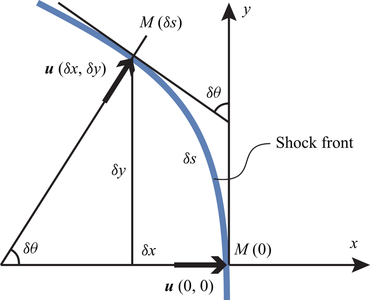
 $t$, we set up a laboratory-fixed local Cartesian coordinate system shown in figure 1, whose origin sits on the shock point defined by
 $\beta$. The positive
 $x$-direction aligns with the instantaneous shock velocity at the origin and the positive
 $y$-direction corresponds to an increase of
 $\beta$ along the shock. The Mach-number profile along the shock may be parametrized as a function of arclength,
 $s$, measured from the origin in the positive
 $y$-direction. In GSD,
 $s$ and
 $\beta$ are related by defining the normalized ray-tube area
 $A$ as
 \begin{equation} A=\frac{\textrm{d} s}{\textrm{d} \beta}. \end{equation}
Local Cartesian coordinates fixed at a point on the shock normal ( $x$-direction) and tangential (
 $y$-direction) to the curve. Downstream velocity vectors and Mach numbers are shown at the origin and a differential nearby point at
 $(\delta x,\delta y)$, whose arclength is
 $\delta s$.

The flow that defines the shock is governed by the 2-D Euler equations:
 \begin{gather} \rho_t+u\rho_x+v\rho_y+\rho(u_x+v_y)=0, \end{gather}
 \begin{gather}\rho(u_t+uu_x+vu_y)+p_x=0, \end{gather}
 \begin{gather}\rho(v_t+uv_x+vv_y)+p_y=0, \end{gather}
 \begin{gather}p_t+up_x+vp_y+\gamma p(u_x+v_y)=0. \end{gather}
2.2.1. Tangential derivatives
In order to obtain an evolution equation analogous to (2.8) that governs the shock motion in two dimensions, all partial derivatives of the flow variables present in (2.11) must be evaluated immediately behind the shock. In particular, this can be done explicitly for the tangential derivatives, i.e. those with respect to  $y$. At the origin, we have, just downstream of the shock,
 $x$ and
 $y$ components of flow velocity (in the laboratory frame), density and pressure given by
 \begin{equation} \left.\begin{gathered} u(0,0) = F^u(M(0)),\quad v(0,0)=0,\\ \rho(0,0)=F^\rho(M(0)),\quad p(0,0)=F^p(M(0)). \end{gathered}\right\} \end{equation}
At a nearby point on the shock  $(\delta x,\delta y)$ with arclength
 $\delta s=\sqrt {\delta x^2+\delta y^2}$, making a tangent angle of
 $\delta \theta$ with the
 $y$-axis (figure 1), these flow quantities become
 \begin{equation} \left.\begin{gathered} u(\delta x,\delta y)= F^u(M(\delta s))\cos(\delta\theta),\quad v(\delta x,\delta y)= F^u(M(\delta s))\sin(\delta\theta),\\ \rho(\delta x,\delta y) = F^\rho(M(\delta s)),\quad p(\delta x,\delta y)=F^p(M(\delta s)), \end{gathered}\right\}\end{equation}
where the Mach number has the Taylor expansion
 \begin{equation} M(\delta s)=M(0)+\left.\frac{\textrm{d} M}{\textrm{d} s}\right|_{(0,0)}\delta s+o(\delta s). \end{equation}
To proceed we make use of the following three limits:
 \begin{equation} \lim_{\delta y\to 0} \delta x/\delta y =0,\quad \lim_{\delta y\to 0} \delta s/\delta y =1, \quad \lim_{\delta y\to 0}\delta \theta/\delta y =\kappa, \end{equation}
where  $\kappa$ is the signed curvature of the shock at the origin. As a result, (2.13) are further Taylor expanded as:
 \begin{equation} \left.\begin{gathered} u(0,0)+\left.\frac{\partial u}{\partial y}\right|_{(0,0)}\delta y=F^u(M(0))+ \left[\frac{\textrm{d} F^u}{\textrm{d} M} \frac{\textrm{d} M}{\textrm{d} s}\right]_{(0,0)}\delta y+o(\delta y),\\ v(0,0)+\left.\frac{\partial v}{\partial y}\right|_{(0,0)}\delta y=F^u(M(0))\delta\theta+o(\delta y),\\ \rho(0,0)+\left.\frac{\partial \rho}{\partial y}\right|_{(0,0)}\delta y=F^\rho(M(0))+ \left[\frac{\textrm{d} F^\rho}{\textrm{d} M} \frac{\textrm{d} M}{\textrm{d} s}\right]_{(0,0)}\delta y+o(\delta y),\\ p(0,0)+\left.\frac{\partial p}{\partial y}\right|_{(0,0)}\delta y=F^p(M(0))+ \left[\frac{\textrm{d} F^p}{\textrm{d} M} \frac{\textrm{d} M}{\textrm{d} s}\right]_{(0,0)}\delta y+o(\delta y). \end{gathered}\right\} \end{equation}
Substituting (2.12) into (2.16) and applying the  $\delta y\to 0$ limit then gives the desired tangential derivatives at the origin,
 \begin{equation} \left.\begin{gathered} \frac{\partial u}{\partial y} = \frac{\textrm{d} F^u}{\textrm{d} M} \frac{\textrm{d} M}{\textrm{d} s},\quad \frac{\partial v}{\partial y} = F^u(M) \kappa,\\ \frac{\partial \rho}{\partial y} = \frac{\textrm{d} F^\rho}{\textrm{d} M} \frac{\textrm{d} M}{\textrm{d} s},\quad \frac{\partial p}{\partial y} = \frac{\textrm{d} F^p}{\textrm{d} M} \frac{\textrm{d} M}{\textrm{d} s}, \end{gathered}\right\} \end{equation}
where we may write
 \begin{equation} \frac{\textrm{d} M}{\textrm{d} s}=\frac{\textrm{d} M}{\textrm{d} \beta}\frac{\textrm{d}\beta}{\textrm{d} s}=\frac{1}{A}\frac{\textrm{d} M}{\textrm{d}\beta}. \end{equation}
Using (2.10) and (2.18), the derivatives in (2.17) can be calculated at time  $t$ provided both the shock-shape and Mach-number profiles are known functions of
 $\beta$.
2.2.2. Time and normal derivatives
Since the shock marker located at the origin at time  $t$ has velocity normal to itself, the time and normal derivatives of flow variables immediately behind the shock are related through the total derivatives:
 \begin{gather} \frac{\textrm{D} u}{\textrm{D} t}=\frac{\textrm{d} F^u}{\textrm{d} M}\left(\frac{\partial M}{\partial t}\right)_\beta= \frac{\partial u}{\partial t}+a_0 M \frac{\partial u}{\partial x}, \end{gather}
 \begin{gather}\frac{\textrm{D} v}{\textrm{D} t}=0=\frac{\partial v}{\partial t}+a_0 M \frac{\partial v}{\partial x}, \end{gather}
 \begin{gather}\frac{\textrm{D}\rho}{\textrm{D} t}=\frac{\textrm{d} F^\rho}{\textrm{d} M}\left(\frac{\partial M}{\partial t}\right)_\beta= \frac{\partial \rho}{\partial t}+a_0 M \frac{\partial \rho}{\partial x}, \end{gather}
 \begin{gather}\frac{\textrm{D} p}{\textrm{D} t}=\frac{\textrm{d} F^p}{\textrm{d} M}\left(\frac{\partial M}{\partial t}\right)_\beta=\frac{\partial p}{\partial t}+a_0 M \frac{\partial p}{\partial x}. \end{gather}
In addition, all the partial derivatives discussed so far satisfy the 2-D Euler equations (2.11). Therefore, substituting (2.12) and (2.17) into (2.11), together with (2.19) gives eight linear equations for eight unknowns, i.e. the  $x$ and
 $t$ partial derivatives of
 $u$,
 $v$,
 $\rho$ and
 $p$. This process is analogous to the derivation of (2.7) for the quasi-1-D problem. In particular, the solution yields
 \begin{equation} \left.\begin{gathered} \frac{\partial u}{\partial t}=\frac{\rho(a^2-u^2)\left(\dfrac{\partial M}{\partial t}\right)_\beta \dfrac{\textrm{d} u}{\textrm{d} M}+a_0M\left[\left(\dfrac{\partial M}{\partial t}\right)_\beta\left(\rho u \dfrac{\textrm{d} u}{\textrm{d} M}+ \dfrac{\textrm{d} p}{\textrm{d} M}\right)+\kappa\rho a^2 u\right]} {\rho[a^2-(u-a_0M)^2]},\\ \frac{\partial p}{\partial t}=\frac{\begin{array}{l} u(a_0M-u)\left(\dfrac{\partial M}{\partial t}\right)_\beta \dfrac{\textrm{d} p}{\textrm{d} M}+a^2\left[\left(\dfrac{\partial M}{\partial t}\right)_\beta\left(\dfrac{\textrm{d} p}{\textrm{d} M}+a_0\rho M \dfrac{\textrm{d} u}{\textrm{d} M}\right) \right.\\ \quad \left.\vphantom{\left(\dfrac{\partial M}{\partial t}\right)_\beta\left(\dfrac{\textrm{d} p}{\textrm{d} M}+a_0\rho M \dfrac{\textrm{d} u}{\textrm{d} M}\right)} +a_0\kappa\rho u M(a_0M-u)\right] \end{array}}{a^2-(u-a_0M)^2}. \end{gathered}\right\} \end{equation}
2.3. Geometrical equivalence
Using (2.20) to expand the expression  $(p_t+\rho a u_t)$ then gives, at any
 $\beta$ and
 $t$,
 \begin{equation} \left(\frac{\partial M}{\partial t}\right)_\beta=-\frac{\dfrac{\kappa a_0M\rho a^2u }{(a+u)}+ \left(\dfrac{a_0M}{a+u}-1\right)\left(\dfrac{\partial p}{\partial t}+\rho a \dfrac{\partial u}{\partial t}\right)}{\dfrac{\textrm{d} p}{\textrm{d} M}+\rho a \dfrac{\textrm{d} u}{\textrm{d} M}}. \end{equation}
An expedited route to arrive at (2.21) is to observe that, because  $v=0$, the momentum equation (2.11c) for
 $v$ decouples from the rest of equations (2.11). Also comparing (2.11) to (2.1), and (2.4a–c) to (2.19), the only difference is that
 $A'/A$ in (2.1) is replaced by
 $\kappa$ in (2.11). As a result, (2.21) is directly analogous to (2.8).
We can conclude that GSD in its complete form given by (2.8) with the  $(p_t+\rho a u_t)$ term retained is equivalent to 2-D Euler if and only if
 \begin{equation} \kappa=\frac{A'}{A}=\frac{1}{a_0MA}\left(\frac{\partial A}{\partial t}\right)_\beta. \end{equation}
By defining  $A$ in 2-D flow as the normalized ray-tube area given in (2.10), Whitham (Reference Whitham2011, equation (8.59)) showed, using the standard
 $\alpha$–
 $\beta$ curvilinear coordinates in GSD, that
 \begin{equation} \frac{\partial \theta}{\partial \beta}=\frac{1}{M}\frac{\partial A}{\partial \alpha}, \end{equation}
where  $\alpha \equiv a_0 t$ is defined as a time-like label for the position of a shock along a ray corresponding to constant
 $\beta$. Equation (2.23) can be shown to be equivalent to (2.22) by noting that
 $\textrm {d} s = A\,\textrm {d}\beta$. For example, the geometrical equivalence for a converging/diverging cylindrical shock of radius
 $r$ is trivially verified by identifying
 $A=A(r)=2{\rm \pi} r$, and thus
 $A'/A=1/r=\kappa$.
Notably, the geometrical equivalence between the evolution of shocks in quasi-1-D and genuine 2-D flows is invariant with respect to the Cartesian coordinates used in § 2.2. Best (Reference Best1993) observed this equivalence and derived an alternative to the original GGSD theory (Best Reference Best1991) resulting from defining the shock velocity to include the local flow velocity component that is tangential to the shock at a time instant. In contrast, in § 2.2, we spatially parametrize the shock using  $\beta$, which labels shock points that propagate locally normal to the shock front. This difference illustrates the somewhat arbitrary definition of the shock velocity. The formulations are physically equivalent. An immediate implication of the geometrical equivalence is that it suffices to consider the quasi-1-D formulation alone in order to construct the shock dynamics in two dimensions, by effectively stacking ray tubes of normalized area
 $A$. We can thus proceed in the following analysis without invoking the 2-D Euler equations.
2.4. A hierarchical expansion of the Euler equations
As shown in §§ 2.1.1 and 2.3, compared to the true Euler equations, the non-uniform details of the flow behind the shock that is missing in the GSD approximation is entirely encapsulated in the quantity  $(p_t+\rho a u_t)$. Therefore a suitable evolutionary model for such a quantity is desired to provide corrections to the GSD description. In the present study, we adapt the GGSD model proposed by Best (Reference Best1991), which expands the Euler equations as a hierarchical system that can be closed at any order. A summary of Best's formulation is outlined here.
The construction begins with assuming sufficient smoothness of quasi-1-D flow and defining
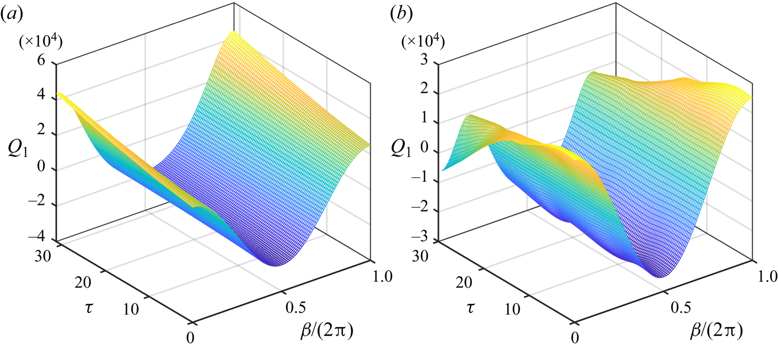
 \begin{equation} Q_n \equiv \frac{\partial^{n-1}}{\partial t^{n-1}}\left(\frac{\partial p}{\partial t}+\rho a \frac{\partial u}{\partial t}\right),\quad n=1,2,\ldots, \end{equation}
evaluated immediately downstream of the shock. It is noted that  $Q_1$ gives the non-uniformity measure, the quantity of interest. Computing the expansion of
 $Q_n$ involves the following convenient differential operator,
 \begin{equation} \mathcal{F}^{i,j}\equiv\frac{\partial^{i+j}}{\partial x^i \partial t^{\,j}}, \quad i,j \in \{0,1,2,\ldots\}, \end{equation}
acting on the flow variables  $p$,
 $u$,
 $\rho$ and
 $a$. Let
 $\xi \in \{p,u,\rho \}$; then along the trajectory of the shock, the total derivative of
 $\xi$ is given by
 \begin{equation} \frac{\textrm{D}}{\textrm{D} t} (\mathcal{F}^{i,j}[\xi]) =\mathcal{F}^{i,j+1}[\xi]+a_0 M \mathcal{F}^{i+1,j}[\xi]. \end{equation}
Further, the following identity for continuously differentiable functions  $A$ and
 $B$,
 \begin{equation} \mathcal{F}^{i,j}[AB]=\sum_{n=0}^{i}\sum_{m=0}^{j} {{i}\choose{n}}{{j}\choose{m}} \mathcal{F}^{n,m}[A]\mathcal{F}^{i-n,j-m}[B], \end{equation}
where  ${i}\choose {n}$ and
 ${j}\choose {m}$ are the binomial operators, allows the Euler equations (2.2) to be differentiated by the operator
 $\mathcal {F}^{i,j}$. This, together with (2.26), forms six linear equations for six unknowns:
 \begin{equation} (\mathcal{F}^{i+1,j}[p],\ \mathcal{F}^{i+1,j}[u],\ \mathcal{F}^{i+1,j}[\rho],\ \mathcal{F}^{i,j+1}[p],\ \mathcal{F}^{i,j+1}[u],\ \mathcal{F}^{i,j+1}[\rho] )^\text{T}, \end{equation}
which can be solved analogously to the derivation of (2.7). The explicit solutions are found in equations (61)–(66) of Best (Reference Best1991). Best's result can be viewed as extensions of the RH condition to the jump in partial derivatives of flow variables across a curved shock, which is a topic that has also been studied by Thomas (Reference Thomas1947), Kanwal (Reference Kanwal1957), Pant (Reference Pant1969), Hornung (Reference Hornung2010), Mölder (Reference Mölder2016) and Emanuel (Reference Emanuel2016, Reference Emanuel2019).
With (2.28) determined, it is then possible to prove by induction the following dependence relation for the partial derivatives:
 \begin{gather} \mathcal{F}^{0,0}[\xi]=\xi(M), \end{gather}
 \begin{gather}\mathcal{F}^{i,j}[\xi] = \mathcal{F}^{i,j}[\xi] \left(M,Q_1,\ldots,Q_{k}, A'/A,\ldots, \frac{\textrm{d}^{k-1}(A'/A)}{\textrm{d} x^{k-1}}\right), \end{gather}
for  $k=i+j$, and
 $i,j\in \{0,1,\ldots \}$. With some manipulations, (2.29) leads to
 \begin{gather} \frac{\textrm{D} M}{\textrm{D} t}=\frac{\textrm{D} M}{\textrm{D} t} (M, Q_1,A'/A ), \end{gather}
 \begin{gather}\frac{\textrm{D} Q_{k+1}}{\textrm{D} t} = \frac{\textrm{D} Q_{k+1}}{\textrm{D} t} \left(M,Q_1,\ldots,Q_{k+2}, A'/A,\ldots, \frac{\textrm{d}^{k}(A'/A)}{\textrm{d} x^{k}}\right). \end{gather}
The explicit expansion of (2.30a) was earlier derived in (2.8) where only first-order partial derivatives of the flow variables were used. In general, higher-order partial derivatives are required to expand (2.30b) and give
 \begin{align} \frac{\textrm{D} Q_{k+1}}{\textrm{D} t} &= -\left[a_0M\frac{\partial^{k+1}}{\partial t^{k+1}} \left(\frac{\rho a^2 u}{a+u}\right)\frac{A'}{A}+a_0M\sum_{i=1}^{k+1}{{k+1}\choose{i}} \frac{\partial^{i}}{\partial t^{i}}\left(\frac{1}{a+u}\right)Q_{k-i+2}\right. \nonumber\\ &\quad \left.+ \, a_0M\frac{\partial^k}{\partial t^k}\left(\frac{\partial(\rho a)}{\partial t} \frac{\partial u}{\partial x}-\frac{\partial(\rho a)}{\partial x}\frac{\partial u}{\partial t}\right)+ \left(\frac{a_0M}{a+u}-1\right)Q_{k+2}\right]. \end{align}
Importantly, (2.29b) and (2.30b) show that the dependence of  $\textrm {D} Q_{k+1}/\textrm {D} t$ upon derivatives of
 $\xi$ of order
 $\leq k+1$ is fully specified by knowing
 $M$ and
 $Q_i$ of order
 $i\leq k+1$. Therefore, for a sequence of coupled nonlinear evolution equations described by (2.30) for
 $k=1,\ldots ,N$, closure can be achieved by truncating the term
 $[a_0M/(a+u)-1]Q_{N+2}$ in (2.31). This results in a closed system of
 $N+2$ nonlinear differential equations for the variables
 $M,Q_1,\ldots ,Q_{N+1}$, which can be integrated in time provided the initial conditions for
 $M,Q_1,\ldots ,Q_{N+1}$ are known.
For instance, it has been shown in § 2.1.1 that truncation at  $Q_1$ in (2.30a) leads to the
 $A$–
 $M$ relation in GSD. And by sampling
 $Q_1$ and its higher derivatives
 $Q_{i\geq 1}$, at time
 $t=0$, the non-uniformity of the initial flow behind the shock is described, which then evolves in time according to the expansion of the Euler equations. Similar to applying the ‘characteristic rule’ in GSD, where the
 $C^+$ characteristic is applied at the shock, the truncation error associated with the present higher-order approach is due to forcing the
 $\textrm {D} Q_N/\textrm {D} t$ equation along the
 $C^+$ characteristic at the shock.
The conditions for convergence of the Mach number  $M$ to the solution obtained from the full 2-D Euler equations as a function of
 $t$, when the truncation number
 $N$ increases, remains an open problem that is addressed incompletely in Best (Reference Best1991, Reference Best1993). We hypothesize that conditions for convergence may be problem-dependent. It is noted that Best's formulation certainly breaks down when the smooth flow assumption is violated, especially if additional discontinuous disturbances that originated downstream and carried by the
 $C^+$ characteristics overtake the shock. Such flow conditions are excluded in the present study.
3. Evolution of a periodic, perturbed planar shock
3.1. A complex-variable formulation
With the truncated GGSD equations established in § 2.4, we can now describe the motion of a slightly perturbed planar shock, parametrized periodically using ray-tube marker  $\beta \in [0,2{\rm \pi} )$ (see § 2.2), by correctly replacing
 $A(x)$ in the quasi-1-D case with the normalized ray-tube area given in (2.10) for a 2-D shock. The
 $2{\rm \pi}$-periodic formulation is convenient for our application to a shock generated by a periodically corrugated piston in § 4. Following Mostert et al. (Reference Mostert, Pullin, Samtaney and Wheatley2018a), we describe the shock shape in a complex
 $z=x+\textrm {i}y$ plane by
 $z=Z(\beta ,t)=X(\beta ,t)+\textrm {i}Y(\beta ,t)$.
By defining ray-tube markers along the shock whose velocity is locally normal to the shock curve, the kinematic equation for the shock profile reads as
 \begin{equation} \left(\frac{\partial Z}{\partial t}\right)_\beta=a_0 M(\beta,t)\hat{n}(\beta,t), \end{equation}
where  $Z\in \mathbb {C}$ is the complex variable that describes the shock curve,
 $a_0$ is the upstream constant sound speed,
 $M$ is the local Mach number and
 $\hat {n}\in \mathbb {C}$ is the unit normal vector aligned with the local shock velocity.
The complex shock profile  $Z$ is now decomposed into a steady flat shock of constant Mach number
 $M_0$ moving in the positive imaginary direction, and its perturbation,
 \begin{equation} Z=Z_0+z(\beta,t),\quad Z_0=\beta+\textrm{i} a_0M_0 t. \end{equation}
It is noted that the unperturbed shock at  $t=0$ here lies on the real axis in the complex plane, and moves in the positive
 $y$-direction. This notation conventionally differs from the discussion in § 2.2.
Further, the unit normal vector,  $\hat {n}=\textrm {i}\hat {s}$, is obtained through a rotation of the unit tangent
 $\hat {s}$, given by
 \begin{equation} \hat{s}=\frac{1}{A(\beta,t)}\frac{\partial Z}{\partial \beta}, \end{equation}
where
 \begin{equation} A(\beta,t)=\left|\frac{\partial Z}{\partial \beta}\right|= \sqrt{\frac{\partial Z}{\partial \beta}\frac{\partial Z^*}{\partial \beta}} \end{equation}
is the normalized ray-tube area in the complex-variable formulation, following (2.10), and  $^*$ denotes complex conjugate. The kinematic equation for the shock-profile perturbation then becomes
 \begin{equation} \frac{\partial z}{\partial t}=\textrm{i}a_0M_0\left[\frac{M}{M_0}\left(1+\frac{\partial z}{\partial \beta}\right) \left|1+\frac{\partial z}{\partial \beta}\right|^{-1}-1\right]. \end{equation}
3.2. Zeroth-order GGSD system: GGSD-0
In order to determine the evolution of the shock shape  $z$, it remains to specify the dynamics of the Mach-number profile
 $M$, which can also be written in the perturbation form
 \begin{equation} M= M_0+m. \end{equation}
Conveniently, using (2.21) with the help of (2.22) and (2.24), we have shown that the Euler equations dictate
 \begin{equation} \frac{\partial m}{\partial t}=-\frac{\dfrac{\rho a^2u\varPhi a_0 M }{(a+u)}+ \left(\dfrac{a_0M}{a+u}-1\right)Q_1}{\textrm{d} p/\textrm{d} M+\rho a (\textrm{d} u/\textrm{d} M)}, \end{equation}
where  $\varPhi \equiv (\partial A/\partial t)/(a_0MA)$ and can be obtained by differentiating (3.4) using (3.1) as
 \begin{equation} \varPhi=\varPhi(Z)=- \left|\frac{\partial Z}{\partial \beta}\right|^{-3} \textrm{Im}\left(\frac{\partial^2Z}{\partial \beta^2}\frac{\partial Z^*}{\partial \beta}\right). \end{equation}
Now, by setting  $Q_1=0$, (3.5) and (3.7) form a set of coupled nonlinear differential equations that describes the shock motion. Such a system corresponds to the zeroth-order truncation of the hierarchical GGSD equations introduced in § 2.4, which gives rise to the
 $A$–
 $M$ relation seen in the GSD model.
There is a subtle difference between GSD and the zeroth-order GGSD system, henceforth referred to as GGSD-0. In GSD, the  $A$–
 $M$ relation, once determined with a unique integration constant, serves as a global constraint over the entire shock profile. For example, Mostert et al. (Reference Mostert, Pullin, Samtaney and Wheatley2018a) derived an expression for the Mach-number profile
 $M$ for a planar shock that is completely determined by the local shock shape
 $Z$, namely,
 $M=M(Z)$. Consequently, (3.5) and (3.7) reduce and combine into a single equation for
 $Z$ that governs the shock shape (see Mostert et al. (Reference Mostert, Pullin, Samtaney and Wheatley2018a), equation (2.9)). In contrast, by separating (3.5) and (3.7) as two independent evolution equations in GGSD-0, the
 $A$–
 $M$ relation applies locally at a given
 $\beta$, allowing the integration constant to differ along the shock. The obvious benefit of such separation is that GGSD-0 is able to handle more general initial value problems that are forbidden in GSD, where the initial shock-shape and Mach-number profiles do not satisfy a global
 $A$–
 $M$ relation everywhere on the shock. Nevertheless if the initial conditions are compatible with a global
 $A$–
 $M$ relation, then GGSD-0 is identical to GSD.
3.2.1. Strong- and weak-shock limits
Here, we simplify (3.7) in the strong- and weak-shock limits, as  $M\to \infty$ and
 $M\to 1$, respectively. This is achieved by utilizing the limiting forms of the RH conditions (2.5) given by
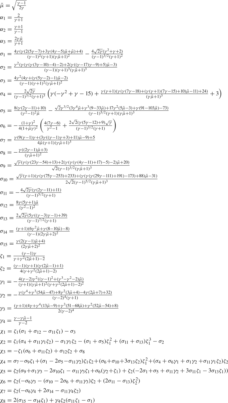
 \begin{equation} u\sim\alpha_1 a_0 M,\quad p\sim \alpha_1 \rho_0 a_0^2 M^2,\quad \rho\sim\alpha_2\rho_0,\quad a\sim\alpha_3a_0M, \end{equation}
as  $M\to \infty$, where
 $\alpha _{1,2,3}$ are constant functions of
 $\gamma$, given in table 1 in appendix A; and similarly,
 \begin{align} u\sim 2\alpha_1 a_0 \varepsilon_{w},\quad p\sim \rho_0a_0^2\left(\frac{1}{\gamma}+2\alpha_1 \varepsilon_{w}\right),\quad \rho\sim\rho_0(1+2\alpha_1\varepsilon_{w}),\quad a\sim a_0\left(1+\frac{2\varepsilon_{w}}{\alpha_2}\right), \end{align}
where  $\varepsilon _{w}\equiv M-1$ and
 $\varepsilon _{w}\to 0$ defines the weak-shock limit. We note that appendix A contains lists of parameters that we use throughout the present study.
Evaluating (3.7) using (3.9a–d) and (3.10a–d), respectively, then yields
 \begin{equation} \left(\frac{\partial M}{\partial t}\right)_\beta=\begin{cases} -\zeta_1 a_0\varPhi M^2+\dfrac{\zeta_2Q_1}{\rho_0a_0^2M}+O(1/M^2), & M\to\infty,\\ -\dfrac{a_0\varPhi \varepsilon_{w}}{2}+\dfrac{ Q_1\varepsilon_{w}}{4\alpha_1\rho_0a_0^2}+O(\varepsilon_{w}^2), & \varepsilon_{w}\to 0, \end{cases}\end{equation}
where  $\zeta _{1,2}$ are again constants listed in table 1 in appendix A. In this asymptotic form, it is assumed that
 $Q_1$ is at least of order
 $O(M^3)$ in the strong-shock limit, and of order
 $O(\varepsilon _{w}^0)$ in the weak-shock limit, for the correction term to be comparable in the respective leading-order expression. Although not necessary for the zeroth-order GGSD model, where the correction is neglected by letting
 $Q_1=0$, such assumptions about the magnitude of
 $Q_1$ will be shown to be essential for deriving the limiting expressions for higher-order GGSD models in the following sections.
For completeness, the zeroth-order GGSD systems in the strong- and weak-shock limits are given by the following closed system:
 \begin{equation} \frac{\partial Z}{\partial t}=\textrm{i}a_0M\frac{\partial Z}{\partial \beta} \left|\frac{\partial Z}{\partial \beta}\right|^{-1},\quad \left(\frac{\partial M}{\partial t}\right)_\beta= \begin{cases} -\zeta_1 a_0\varPhi M^2, & M\to\infty,\\ -\dfrac{a_0\varPhi}{2}(M-1), & M\to 1. \end{cases}\end{equation}
3.3. First-order GGSD system: GGSD-1
As discussed in § 2.4, corrections to GGSD-0 can be made by including higher-order equations that capture the evolution of  $Q_1$. In this section, we obtain the GGSD-1 model explicitly in the weak- and strong-shock limits.
The evolution of  $Q_1$ following the shock trajectory in the quasi-1-D flow is governed by (2.31) with
 $k=0$. Using the present complex-variable formulation, the total time derivative,
 $\textrm {D} Q_1/\textrm {D} t$, described by (2.31) directly equates to the partial time derivative tracing a fixed ray-tube marker
 $\beta$, namely,
 $(\partial Q_1/\partial t)_\beta$. Similarly, the full differential
 $\textrm {d} x$ that appears in
 $A'$ is now understood as the differential distance travelled by the shock in the ray-tube direction, i.e.
 \begin{equation} \textrm{d} x=a_0 M(\beta, t)\,\textrm{d} t,\quad \frac{A'}{A}=\frac{1}{a_0 MA}\left(\frac{\partial A}{\partial t}\right)_\beta=\varPhi, \end{equation}
where  $\varPhi$ is given in (3.8). Now substituting (3.13a,b) into (2.31) yields
 \begin{align} \left(\frac{\partial Q_1}{\partial t}\right)_\beta &= -a_0 M\left[\frac{\partial}{\partial t} \left(\frac{\rho a^2 u}{a+u}\right) \varPhi+\frac{\partial(\rho a)}{\partial t} \frac{\partial u}{\partial x}-\frac{\partial(\rho a)}{\partial x} \frac{\partial u}{\partial t} \right.\nonumber\\ &\quad \left.+\,\frac{\partial}{\partial t} \left(\frac{1}{a+u}\right)Q_1+\left(\frac{1}{a+u}-\frac{1}{a_0M}\right)Q_2\right]. \end{align}
Expanding (3.14) and noting that  $a=\sqrt {\gamma p/\rho }$ produces first-order partial derivatives of
 $\rho$,
 $u$ and
 $p$ with respect to
 $t$ and
 $x$, which are found as a subset of solution (2.28), where
 $i=j=0$. Therefore, in view of (2.29b), (3.14) is fully specified knowing
 $M$,
 $Q_1$ and
 $\varPhi$, except for the last term that contains
 $Q_2$. Hence truncation at
 $Q_2=0$ provides closure. GGSD-1 then comprises (3.5), (3.7) and (3.14) with
 $Q_2=0$.
3.3.1. The weak-shock limit
The full expansion of  $\mathcal {F}^{0,1}[\xi ^*]$ and
 $\mathcal {F}^{1,0}[\xi ^*]$, where
 $\xi ^*\in \{\rho , u, p, a\}$, can be obtained as a subset from the solution process to the arrival of (2.28). Using the asymptotic forms (3.10a–d) and (3.11), these first-order partial derivatives, listed in (B 1)–(B 4) of appendix B, simplify in the weak-shock limit as
 $\varepsilon _{w}=M-1\to 0$. It is noted that the leading-order behaviour of all eight partial derivatives in this limit relies on the assumption that
 $Q_1\sim O(\varepsilon _{w}^0)\sim O(1)$, which is consistent with the observation made with (3.11) when
 $Q_1\neq 0$ is allowed.
Substituting (3.10a–d) and (B 1)–(B 4) into (3.14) then gives the leading-order evolution of  $Q_1$ in the weak-shock limit,
 \begin{equation} \left(\frac{\partial Q_1}{\partial t}\right)_\beta=\frac{Q_1}{2} \left(\frac{Q_1}{\alpha_1\rho_0a_0^2} -a_0\varPhi\right)+ Q_2\varepsilon_{w}+O(\varepsilon_{w}), \end{equation}
where the correction term  $Q_2\varepsilon _{w}$ enters only if
 $Q_2\sim O(1/\varepsilon _{w})$ at least. However, closure of the GGSD system at first order demands
 $Q_2=0$; and therefore combining (3.5), (3.11) and (3.15) completes the weak-shock limiting GGSD-1 equations as follows:
 \begin{equation} \left.\begin{gathered} \frac{\partial Z}{\partial t}=\textrm{i}a_0M\frac{\partial Z}{\partial \beta}\left|\frac{\partial Z}{\partial \beta}\right|^{-1},\\ \frac{\partial M}{\partial t}=\left(-\frac{a_0\varPhi}{2}+\frac{ Q_1}{4\alpha_1\rho_0a_0^2}\right)(M-1),\\ \frac{\partial Q_1}{\partial t}=\frac{Q_1}{2} \left(\frac{Q_1}{\alpha_1\rho_0a_0^2} -a_0\varPhi\right). \end{gathered}\right\} \end{equation}
3.3.2. The strong-shock limit
Analogous analysis can be carried out for the strong-shock limit. Substituting (3.9a–d) into the general solution of the first-order partial derivatives leads to the strong-shock limits of (B 1)–(B 4) in appendix B, where  $M'$ is understood similarly as in (3.13a,b), such that, upon using (3.11), one has
 \begin{equation} M'=\frac{\textrm{d} M}{\textrm{d} x}=\frac{1}{a_0 M}\left(\frac{\partial M}{\partial t}\right)_\beta\sim -\zeta_1\varPhi M+ \frac{\zeta_2Q_1}{\rho_0a_0^3M^2}. \end{equation}
It is thus observed that  $M'\sim O(M)$, so the
 $M'$ notation is preferably kept in (B 1)–(B 4) and henceforth for convenient identification of the leading-order behaviour.
Again, substituting (3.9a–d), (B 1)–(B 4) and (3.17) into (3.14) yields the limiting  $Q_1$ equation,
 \begin{equation} \left(\frac{\partial Q_1}{\partial t}\right)_\beta=\gamma_1 \rho_0a_0^4\varPhi^2 M^4+\gamma_2a_0 M \varPhi Q_1+\frac{\gamma_3 Q_1^2}{\rho_0a_0^2M^2}+\gamma_4 Q_2+O(M^3), \end{equation}
where  $\gamma _{1,2,3,4}$ are coefficients listed in table 1 in appendix A. Setting
 $Q_2=0$, which otherwise is assumed as
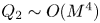 $Q_2\sim O(M^4)$, (3.18) is joined with (3.5) and (3.11) to form the GGSD-1 equations in the strong-shock limit:
 \begin{equation} \left.\begin{gathered} \frac{\partial Z}{\partial t}=\textrm{i}a_0M\frac{\partial Z}{\partial \beta}\left|\frac{\partial Z}{\partial \beta}\right|^{-1},\\ \frac{\partial M}{\partial t}=-\zeta_1a_0\varPhi M^2+\frac{\zeta_2Q_1}{\rho_0a_0^2M},\\ \frac{\partial Q_1}{\partial t}=\gamma_1 \rho_0a_0^4\varPhi^2 M^4+\gamma_2a_0\varPhi M Q_1+\frac{\gamma_3 Q_1^2}{\rho_0a_0^2M^2}. \end{gathered}\right\} \end{equation}
3.4. Second-order GGSD system: GGSD-2
The second-order GGSD system can be similarly established by incorporating the evolution of  $Q_2$, governed by (2.31), where
 $k=1$ and
 $Q_3=0$:
 \begin{align} \left(\frac{\partial Q_2}{\partial t}\right)_\beta &= -a_0 M\varPhi\frac{\partial^2}{\partial t^2} \left(\frac{\rho a^2 u}{a+u}\right)-a_0M\left[\frac{\partial^{2}}{\partial t^{2}} \left(\frac{1}{a+u}\right)Q_{1}+2\frac{\partial}{\partial t}\left(\frac{1}{a+u}\right)Q_{2}\right] \nonumber\\ &\quad -a_0M\frac{\partial}{\partial t}\left(\frac{\partial(\rho a)}{\partial t}\frac{\partial u}{\partial x}- \frac{\partial(\rho a)}{\partial x}\frac{\partial u}{\partial t}\right)-\left(\frac{a_0 M}{a+u}-1\right)Q_3. \end{align}
Again, without the  $Q_3$ correction, the rest of (3.20) is fully determined because the second-order partial derivatives,
 $\{\mathcal {F}^{n,m}[\xi ^*]: \xi ^*\in \{\rho , u, p, a\},\ n+m=2\}$, only depends on
 $M$,
 $Q_1$,
 $Q_2$ and ultimately
 $Z$. To see this, the apparent dependence of
 $(A'/A)'$ in (2.29b) for quasi-1-D flow here becomes
 \begin{equation} \frac{\textrm{d}}{\textrm{d} x}\left(\frac{A'}{A}\right)=\frac{1}{a_0M}\left(\frac{\partial \varPhi}{\partial t}\right)_\beta, \end{equation}
which can be evaluated according to the definition of  $\varPhi$, (3.8), after obtaining the partial derivatives,
 $Z_{\beta t}$ and
 $Z_{\beta \beta t}$, from differentiating (3.1) and its complex conjugate with respect to
 $\beta$, once and twice, respectively. As a result, one defines
 $\varPsi \equiv (A'/A)'$ and arrives at
 \begin{equation} \varPsi=\varPsi(Z,M)=-\varPhi^2-\frac{1}{A^4M}\left[A^2\frac{\partial^2 M}{\partial \beta^2}-\textrm{Re} \left(\frac{\partial^2Z}{\partial \beta^2}\frac{\partial Z^*}{\partial \beta}\right)\frac{\partial M}{\partial \beta}\right], \end{equation}
where  $A=|\partial Z/\partial \beta |$. The explicit expansion of (3.20) is determined next in the weak- and strong-shock limits.
3.4.1. The weak-shock limit
In order to obtain the various second-order partial derivatives involved in (3.20), the shock local acceleration is also required. This is computed by differentiating (3.11) (recall  $\epsilon =M-1)$ as follows:
 \begin{align} \frac{\partial^2 \varepsilon_{w}}{\partial t^2}=\frac{1}{4\alpha_1\rho_0^2a_0^2}\left\{\varepsilon_{w} \frac{\partial Q_1}{\partial t}+Q_1\frac{\partial \varepsilon_{w}}{\partial t}-2\alpha_1 \rho_0^2a_0^3 \left[\varPhi\frac{\partial \varepsilon_{w}}{\partial t}+a_0\varepsilon_{w}(1+\varepsilon_{w})\varPsi\right]\right\} \sim O(\varepsilon_{w}), \end{align}
where  $\partial Q_1/\partial t$,
 $\partial \varepsilon _{w}/\partial t$,
 $\varPhi$ and
 $\varPsi$ are known due to (3.15), (3.11), (3.8) and (3.22).
With (3.10a–d), (B 1)–(B 4), (3.22) and (3.23) available, expressions for the required second-order partial derivatives of flow variables are Taylor-expanded around  $\varepsilon _{w}=0$, yielding the leading-order behaviour given in (B 5)–(B 8) of appendix B. We note that
 $Q_2\sim O(1/\varepsilon _{w})$ and recall (3.15). Finally, substituting (3.10a–d) and (B 5)–(B 8) into (3.20), while letting
 $Q_3=0$, produces the evolution equation for
 $Q_2$ as
 $\epsilon \to 0$, which is then joined to (3.5), (3.11) and (3.15) to form the following GGSD-2 system in the weak-shock limit:
 \begin{equation} \left.\begin{gathered} \frac{\partial Z}{\partial t}=\textrm{i}a_0M\frac{\partial Z}{\partial \beta}\left|\frac{\partial Z}{\partial \beta}\right|^{-1},\\ \frac{\partial M}{\partial t}=(M-1)\left(-\frac{a_0\varPhi}{2}+\frac{Q_1}{4\alpha_1\rho_0a_0^2}\right),\\ \frac{\partial Q_1}{\partial t}=\frac{Q_1}{2} \left(\frac{Q_1}{\alpha_1\rho_0a_0^2} -a_0\varPhi\right)+(M-1)Q_2,\\ \frac{\partial Q_2}{\partial t}=\frac{[(\gamma+1)Q_1-2\rho_0a_0^3\varPhi]Q_2}{4\rho_0a_0^2}. \end{gathered}\right\} \end{equation}
3.4.2. The strong-shock limit
As an analogy to (3.23), the second time derivative  $\partial ^2 M/\partial t^2$ is prepared first,
 \begin{equation} \frac{\partial^2 M}{\partial t^2}=-\zeta_1 a_0M\left(a_0\varPsi M^2+2\varPhi \frac{\partial M}{\partial t}\right)+\frac{\zeta_2}{\rho_0a_0^2M^2} \left(M\frac{\partial Q_1}{\partial t}-Q_1\frac{\partial M}{\partial t}\right), \end{equation}
where  $\partial Q_1/\partial t$,
 $\partial M/\partial t$,
 $\varPhi$ and
 $\varPsi$ are found in (3.18), (3.11), (3.8) and (3.22), respectively. However, here in the strong-shock limit, it is more convenient to further attain
 $M''\equiv \textrm {d}(M')/\textrm {d} x$, fully expanded using (3.13a,b), (3.11), (3.18) and (3.25) as
 \begin{equation} M'' = [(\zeta_1^2+\gamma_1\zeta_2 )\varPhi^2-\zeta_1\varPsi ]M + \frac{(\zeta_1+\gamma_2)\zeta_2\varPhi Q_1}{\rho_0a_0^3M^2} + \frac{\zeta_2(\gamma_3-2\zeta_2)Q_1^2}{\rho_0^2a_0^6M^5} + \frac{\zeta_2\gamma_4Q_2}{\rho_0a_0^4M^3}. \end{equation}
Consequently,  $M''\sim M'\sim O(M)$ is established.
Next, the second-order partial derivatives contributing to the expansion of  $\partial Q_2/\partial t$ can be expressed in terms of
 $M''$, for the same reason that
 $M'$ is preferred in (B 1)–(B 4). The explicit asymptotic formulae are reported in (B 5)–(B 8) in appendix B. After evaluating (3.20) using (B 5)–(B 8) in the strong-shock limit, the GGSD-2 equations follow:
 \begin{equation} \left.\begin{gathered} \frac{\partial Z}{\partial t}=\textrm{i}a_0M\frac{\partial Z}{\partial \beta}\left|\frac{\partial Z}{\partial \beta}\right|^{-1},\\ \frac{\partial M}{\partial t}=-\zeta_1a_0\varPhi M^2+\frac{\zeta_2Q_1}{\rho_0a_0^2M},\\ \frac{\partial Q_1}{\partial t}=\gamma_1 \rho_0a_0^4\varPhi^2 M^4+\gamma_2a_0\varPhi M Q_1+ \frac{\gamma_3 Q_1^2}{\rho_0a_0^2M^2}+\gamma_4Q_2,\\ \frac{\partial Q_2}{\partial t}=\rho_0a_0^5M^5 (\chi_1\varPhi\varPsi+\chi_2\varPhi^3 )-a_0^2M^2 (\chi_3\varPsi+\chi_4\varPhi^2 )Q_1-\frac{\chi_5\varPhi Q_1^2}{\rho_0a_0M}\\ \hspace{-5.8pc}+\frac{\chi_6Q_1^3}{\rho_0^2a_0^4M^4}+\frac{\chi_7Q_1Q_2}{\rho_0a_0^2M^2}+\chi_8a_0\varPhi M Q_2, \end{gathered}\right\} \end{equation}
where  $\chi _{1,2,\ldots ,8}$ are again constant functions of
 $\gamma$ listed in table 1 in appendix A. This completes the derivation of the shock-evolution equations used presently.
3.5. Unbounded linear growth
We now demonstrate that the zeroth-order GGSD system is linearly stable, whilst including the  $Q_1$ correction in the first-order GGSD equations leads to linearized solutions that exhibit unbounded growth in time. Equations (3.16) and (3.19) are expanded around a plane shock of constant Mach number
 $M_0$, and consequently a steady downstream flow with
 $Q_1=Q_{10}$. The plane shock motion is described by
 $Z_0=\beta +\textrm {i} a_0M_0 t$, and the following rescaled perturbation fields are considered,
 \begin{align} Z=Z_0+z_1(\beta,t)\delta + \cdots,\quad M=M_0+m_1(\beta,t)\delta + \cdots,\quad Q_1=Q_{10}+q_1(\beta,t)\delta + \cdots, \end{align}
where  $\delta \ll 1$ is the dimensionless perturbation size, and the subscript ‘1’ is used to distinguish from unscaled variables used in (3.2a,b) and (3.6). The
 $\delta \to 0$ asymptotic behaviour is explored next for the limiting equations (3.16) and (3.19), corresponding to weak and strong shocks where the respective
 $M_0\to 1$ and
 $M_0\to \infty$ limits have been applied. Substituting (3.28a–c) into (3.16) and (3.19) yields, at order
 $O(\delta ^0)$, that, for both weak and strong shocks,
 \begin{equation} Q_{10}=0, \end{equation}
implying that the linear behaviour of the shock is fully described by the zeroth-order GGSD system. Further, at order  $O(\delta )$, one has
 \begin{gather} \frac{\partial z_1}{\partial t}=\frac{\textrm{i} a_0 M_0}{2} \left(\frac{\partial z}{\partial \beta}-\frac{\partial z^*}{\partial \beta}\right)+\textrm{i} a_0 m_1, \end{gather}
 \begin{gather}\frac{\partial m_1}{\partial t}=\begin{cases} \dfrac{\zeta_2 q_1}{\rho_0a_0^2 M_0 }-\dfrac{\textrm{i}\zeta_1 a_0 M_0^2}{2} \left(\dfrac{\partial^2 z_1}{\partial \beta^2}-\dfrac{\partial^2 z_1^*}{\partial \beta^2}\right), & M_0\to\infty,\\ \dfrac{(M_0-1)q_1}{4\alpha_1\rho_0 a_0^2}- \dfrac{\textrm{i}a_0(M_0-1)}{4}\left(\dfrac{\partial^2 z_1}{\partial \beta^2}-\dfrac{\partial^2 z_1^*}{\partial \beta^2}\right), & M_0\to 1, \end{cases} \end{gather}
 \begin{gather}\frac{\partial q_1}{\partial t}=0. \end{gather}
As a result of (3.30c),  $q_1$ is a constant function of
 $\beta$ to be determined from the initial conditions of the flow immediately behind the shock, namely,
 \begin{equation} q_1(\beta,t)=q_1(\beta,0),\quad \forall\ t>0. \end{equation}
By differentiating (3.30a) with respect to  $\beta$, (3.30b) can be cast into
 \begin{equation} \frac{\partial m_1}{\partial t}=\begin{cases} -\dfrac{\zeta_1M_0}{2}\dfrac{\partial}{\partial t} \left(\dfrac{\partial z_1}{\partial \beta}+\dfrac{\partial z_1^*}{\partial \beta}\right)+ \dfrac{\zeta_2 q_1}{\rho_0a_0^2 M_0 }, & M_0\to\infty,\\ -\dfrac{(M_0-1)}{4M_0}\dfrac{\partial}{\partial t} \left(\dfrac{\partial z_1}{\partial \beta}+\dfrac{\partial z_1^*}{\partial \beta}\right)+ \dfrac{(M_0-1) q_1}{4\alpha_1\rho_0a_0^2 }, & M_0\to 1, \end{cases} \end{equation}
which can be integrated with respect to  $t$ because of (3.31) to give
 \begin{equation} m_1=\begin{cases} -\dfrac{\zeta_1M_0}{2}\left(\dfrac{\partial z_1}{\partial \beta}+ \dfrac{\partial z_1^*}{\partial \beta}\right)+\dfrac{\zeta_2 q_1}{\rho_0a_0^2 M_0}t+f(\beta), & M_0\to\infty,\\ -\dfrac{M_0-1}{4}\left(\dfrac{\partial z_1}{\partial \beta}+\dfrac{\partial z_1^*}{\partial \beta}\right)+ \dfrac{(M_0-1) q_1}{ 4\alpha \rho_0a_0^2 }t+f(\beta), & M_0\to 1, \end{cases} \end{equation}
where  $f(\beta )$ is prescribed from the initial Mach-number profile
 $m_1(\beta ,0)$. Further, (3.33) is substituted into (3.30a), to show
 \begin{equation} \frac{\partial z_1}{\partial \tau}=\begin{cases} \textrm{i}\left(\dfrac{1-\zeta_1}{2}\dfrac{\partial z}{\partial \beta}-\dfrac{1+\zeta_1}{2} \dfrac{\partial z^*}{\partial \beta}+\dfrac{\zeta_2 q_1 \tau}{\rho_0a_0^3M_0^3} + \dfrac{f}{M_0}\right), & M_0\to\infty,\\ \textrm{i}\left(\dfrac{3-M_0}{4}\dfrac{\partial z_1}{\partial \beta}-\dfrac{1+M_0}{4} \dfrac{\partial z_1^*}{\partial \beta}+\dfrac{(M_0-1) q_1 \tau}{4\alpha_1\rho_0a_0^3} + f\right), & M_0\to 1, \end{cases}\end{equation}
where  $\tau =a_0M_0t$ is a time-like length unit defined for convenience. The solution for
 $z_1$ can be obtained using a Fourier expansion in
 $\beta$,
 \begin{equation} z_1(\beta,\tau)=\sum_{n=-\infty}^{\infty}\hat{z}_n(\tau)\,\textrm{e}^{\textrm{i}n\beta},\quad q_1(\beta)=\sum_{n=-\infty}^{\infty}\hat{q}_n\,\textrm{e}^{\textrm{i}n\beta},\quad f(\beta)=\sum_{n=-\infty}^{\infty}\hat{f}_n\,\textrm{e}^{\textrm{i}n\beta}, \end{equation}
in both (3.34) and its complex conjugate. This yields the following second-order ordinary differential equations for the Fourier coefficients  $\hat {z}_n$:
 \begin{equation} \frac{\textrm{d}^2 \hat{z}_n}{\textrm{d}\tau^2}=\begin{cases} -\zeta_1 n^2\hat{z}_n+\textrm{i}\left[\dfrac{\zeta_2(1-n\tau)\hat{q}_n}{\rho_0a_0^3M_0^3} -\dfrac{n\hat{f}_n}{M_0}\right], & M_0\to\infty,\\ -\dfrac{M_0-1}{2} n^2\hat{z}_n +\textrm{i} \left[\dfrac{(M_0-1)(1-n\tau)\hat{q}_n}{4\alpha_1\rho_0a_0^3}-n\hat{f}_n\right], & M_0\to 1, \end{cases} \end{equation}
whose solutions are given by
 \begin{align} \hat{z}_n=\begin{cases} A_n \cos\left(\sqrt{\zeta_1} n \tau \right)+B_n \sin\left(\sqrt{\zeta_1} n\tau\right)+\textrm{i}(C_n \tau +D_n), & M_0\to\infty,\\ A_n \cos\left(\sqrt{ \frac12 (M_0-1)} \, n \tau \right)+B_n \sin\left(\sqrt{ \frac12 (M_0-1)} \, n \tau \right)+ \textrm{i}(C_n \tau +D_n), & M_0\to 1, \end{cases} \end{align}
where  $A_n$ and
 $B_n$ are constants to be determined from the initial shock shape
 $z_1(\beta , 0)$, and from the particular linear source term,
 \begin{equation} C_n=\begin{cases} \dfrac{-\zeta_2\hat{q}_n}{\zeta_1 \rho_0a_0^3M_0^3n^2},\\ \dfrac{-\hat{q}_n}{2\alpha_1\rho_0a_0^3n}, \end{cases} D_n=\begin{cases} \dfrac{\zeta_2\hat{q}_n-\rho_0a_0^3M_0^2n\hat{f}_n}{\zeta_1\rho_0a_0^3M_0^3n^2}, & M_0\to\infty,\\ \dfrac{1}{2n^2}\left(\dfrac{\hat{q}_n}{\alpha_1\rho_1a_0^3}-\dfrac{4n\hat{f}_n}{M_0-1}\right), & M_0\to 1. \end{cases} \end{equation}
Finally, substituting (3.38a,b) into (3.35a–c) and subsequently (3.33) completes the general solutions for  $z_1$ and
 $m_1$.
If a shock is given an initial Mach-number perturbation, and the flow that produced the perturbation persists, a reasonable physical expectation could be that the shock develops a shape perturbation that grows linearly in the imaginary (shock-normal) direction with time. In the present theory, the forcing behind the shock is represented by the quantities  $Q_1$ and
 $Q_2$. From (3.38a,b) and (3.33), for a flow with
 $Q_1 = 0$, where the shock is given an initial Mach-number perturbation and moves into a uniform medium, linear theory produces a solution that is the same as would be predicted by the linear zeroth-order GGSD (or GSD) model, where
 $Q_1$ plays no role. Here the shock motion consists of stable oscillations in the shock shape that are normal to its unperturbed profile, and with fixed amplitude and frequency.
For the present piston-generated shock, where the shock moves into a uniform medium but is subject to an initial perturbation with  $Q_1 \neq 0$, linearized first-order GGSD predicts, in addition to oscillatory behaviour, a growth term that is linear in time for both the shock-shape and Mach-number perturbations, consistent with the above-stated expectation. Hence the linearized GGSD model suggests unbounded shock acceleration driven by non-uniformities (that is, non-zero
 $Q_1$) behind the shock. This amplitude growth, however, does not occur in alternative theories (e.g. Freeman Reference Freeman1957). In the sequel it will be shown that linear growth in time is in fact controlled by nonlinear behaviour.
4. Evolution of shock generated by a slightly corrugated piston
We now use the GGSD equations to investigate the evolution and nonlinear stability of a shock generated by an impulsively started piston of sinusoidal shape. The GGSD approach is chosen over numerical solutions of the full Euler equations. Shock-capturing Euler methods contain their own shock modelling in the form of highly nonlinear artificial dissipation focused on the shock profile, making them a questionable choice for investigating the long-time evolution of tiny disturbances to a plane shock. A shock-fitting method would seem ideal but is difficult to implement at order sufficiently high to accurately capture spontaneous singularity formation.
4.1. Base motion
The shock considered in this study is produced by the impulsive motion of a piston from rest, whose velocity as a complex variable in the  $Y$-direction is given by
 \begin{equation} U_p(t)=U \textrm{H}(t)\,\textrm{e}^{\textrm{i}{\rm \pi}/2}, \end{equation}
where  $U>0$ is the constant speed that the piston gains and
 $\textrm {H}(t)$ is the Heaviside function. For a piston with flat surface located at
 $Y=0$ moving into a uniform stationary medium, such an impulse in the limit of
 $U\to \infty$ or
 $U\to 0$ generates a normal plane shock of constant Mach number,
 \begin{equation} M_0=\begin{cases} \dfrac{U}{\alpha_1 a_0}, & M \to \infty,\\ 1+\dfrac{U}{2a_0\alpha_1}, & M \to 1, \end{cases} \end{equation}
after applying the strong- and weak-shock limits of the RH conditions (3.9a–d) and (3.10a–d). The base motion of the shock in the form of (3.2a,b) is thus established, namely,
 \begin{equation} Z_0=\beta+\textrm{i}a_0M_0t. \end{equation}
It is noted that, for  $t>0$, the shock-processed flow between the piston and shock front is uniform with velocity also given by (4.1). To proceed, non-dimensional variables are used according to a reference length scale
 $L_0$, such that
 $2{\rm \pi} L_0$ is the initial perturbation wavelength; a reference velocity
 $a_0$ and density
 $\rho _0$. The time and pressure scales are thus derived as
 $L_0/a_0$ and
 $\rho _0a_0^2$, respectively.
4.2. Initial values for $Z$ and $M$


Next, a cosine perturbation of small amplitude  $\epsilon \ll 1$ is imposed to the piston surface. Freeman (Reference Freeman1955) showed that the corresponding shock generated by such a corrugated piston must have the same initial shape profile as the piston surface. Therefore, at
 $t=0^+$, the shock shape is prescribed as
 \begin{equation} Z(\beta,0^+)=Z_0(\beta,0^+)+z(\beta,0^+)=\beta+\textrm{i}\epsilon \cos(\beta). \end{equation}
In order to obtain the initial Mach-number distribution of this curved shock produced by the same piston impulse (4.1), it is noted that, along the infinitely thin layer of fluid sandwiched between the piston and shock at  $t=0^+$, only the piston velocity component locally normal to the boundary is transferred into the fluid, whereas the tangential component slips through the fluid under the present Euler description. Therefore, in the laboratory frame where the piston velocity (4.1) is measured, the initial boundary fluid velocity distribution follows as the projection of piston velocity onto the unit normal vector given in (3.3), leading to
 \begin{equation} u_0\equiv u(\beta,0^+)=\begin{cases} \dfrac{\alpha_1 M_0}{\sqrt{\epsilon ^2 \sin ^2(\beta )+1}}, & M_0\to\infty,\\ \dfrac{2 \alpha_1 (M_0-1)}{\sqrt{\epsilon ^2 \sin ^2(\beta )+1}}, & M_0\to 1, \end{cases} \end{equation}
where the base motion Mach number  $M_0$ found in (4.2) is used as the input parameter. Because the shock curve coincides with the piston surface at
 $t=0^+$, the normal RH conditions can be applied again to convert (4.5) into the required initial values of Mach number,
 \begin{equation} M(\beta,0^+)=\begin{cases} \dfrac{M_0}{\sqrt{\epsilon^2\sin^2(\beta)+1}}, & M_0\to\infty,\\ 1+\dfrac{M_0-1}{\sqrt{\epsilon^2\sin^2(\beta)+1}}, & M_0\to 1. \end{cases} \end{equation}
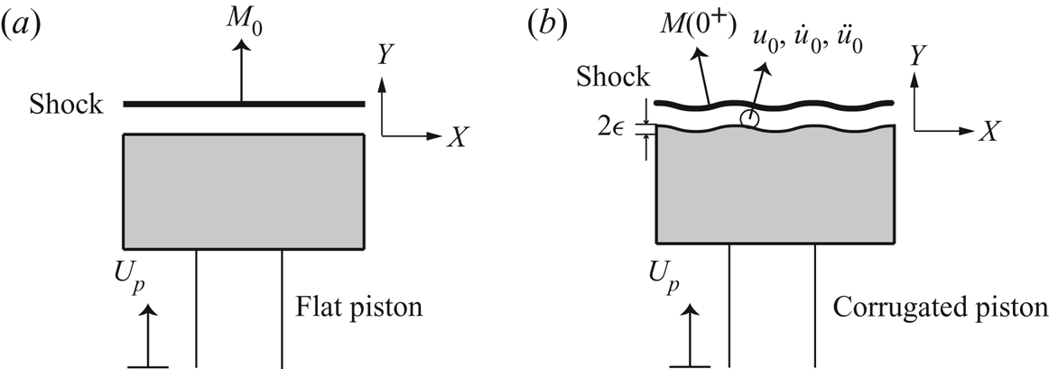
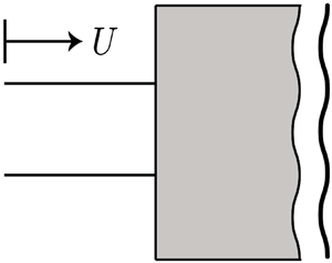
A schematic comparison between shocks generated by flat and corrugated pistons is shown in figure 2, where the infinitesimal layer of shock-processed flow attached to the piston boundary at  $t=0^+$ is illustrated with kinematic quantities including acceleration and jerk that are discussed in the next section.
Shock generated by (a) a flat piston and (b) a corrugated piston of perturbation amplitude  $\epsilon$, at time
 $t=0^+$. Both pistons share the same velocity
 $U_p$, giving a constant Mach number
 $M_0$ when the piston is flat. In (b) the Mach-number profile is
 $M(\beta ,0^+)$. The flow between the piston and the shock is uniform in (a), but non-uniform with initial velocity
 $u_0$, acceleration
 $\dot {u}_0$ and jerk
 $\ddot {u}_0$ in (b).

4.3. Initial values for $Q_1$ and $Q_2$


To complete the GGSD initial value problem formulation for the piston-generated shock, it remains to determine  $Q_1$ and
 $Q_2$ at
 $t=0^+$. This is achieved by utilizing two kinematic conditions of the boundary flow, about its initial acceleration
 $\dot {u}_0$ and jerk
 $\ddot {u}_0$ in the shock-normal direction. For each
 $\beta$, these quantities take the form of a full derivative moving with the piston,
 \begin{gather} \dot{u}_0(\beta)=u_t(\beta,0^+)+u_0u_x(\beta,0^+), \end{gather}
 \begin{gather}\ddot{u}_0(\beta)=\left.\frac{\partial (u_t+u u_x)}{\partial t}\right|_{t=0^+}+u_0\left.\frac{\partial (u_t+u u_x)}{\partial x}\right|_{t=0^+}, \end{gather}
where  $u_0$ is derived in (4.5), and the first- and second-order derivatives of
 $u$ are given in (B 1)–(B 4) and (B 5)–(B 8), respectively, in appendix B.
Expanding (4.7a) using (B 2a) and (B 2b), while in the strong-shock case expressing  $M'$ in terms of
 $Q_1$ via (3.17), leads to the initial values for
 $Q_1$,
 \begin{align} Q_1(\beta,0^+)=\begin{cases} \dfrac{M(\beta,0^+)^2}{\zeta_2}\left[\zeta_1\varPhi M+\dfrac{4 \gamma M (u_0-1) \varPhi +(\gamma +1)^2 \dot{u}_0}{2 (\gamma +1) (4 M-3 u_0)}\right]_{t=0^+}, & M_0\to \infty,\\ \left.\dfrac{4 (M-1) \varPhi (-2 \gamma +(3 \gamma -1) u_0+2)+2 (\gamma +1)^2 \dot{u}_0}{(\gamma +1)^2 (2 M-u_0-1)}\right|_{t=0^+}, & M_0\to 1, \end{cases} \end{align}
where, in both limits,  $\varPhi |_{t=0^+}$ can be evaluated from its definition (3.8) using the initial shock profile (4.4) as
 \begin{equation} \varPhi(\beta,0^+)=\frac{\epsilon \cos (\beta )}{(\epsilon ^2 \sin ^2(\beta )+1)^{3/2}}. \end{equation}
Substituting (4.5), (4.6) and (4.9) into (4.8) completes the expression. Specifically, evaluating  $Q_1(\beta ,0^+)$ at
 $\epsilon =0$ shows that
 \begin{equation} Q_1(\beta,0^+)|_{\epsilon=0}=\begin{cases} \dfrac{(\gamma+1)M_0\dot{u}_0(\beta)}{(8-6\alpha_1)\zeta_2}, & M_0\to\infty,\\ \dfrac{2\dot{u}_0(\beta)}{1-2(\alpha_1-1)(M_0-1)}, & M_0\to 1. \end{cases} \end{equation}
As discussed in § 4.1, the unperturbed flow between the piston and shock is uniform, implying that  $Q_1(\beta ,0^+)|_{\epsilon =0}=0$ for all
 $\beta$. Therefore, it is concluded that
 $\dot {u}_0(\beta )=0$, that is, the initial boundary flow is acceleration-free. Hence
 $Q_1(\beta ,0^+)$ simplifies to yield the following leading-order behaviour as
 $\epsilon \to 0$:
 \begin{equation} Q_1(\beta,0^+)\sim\begin{cases} \dfrac{M_0^3 \epsilon \cos (\beta ) [\alpha _1 (3 (\gamma +1) \zeta _1-2 \gamma )-4 (\gamma +1) \zeta _1]}{(3 \alpha _1-4) (\gamma +1) \zeta _2}, & M_0\to \infty,\\ \dfrac{8 (M_0-1)\epsilon (1-\gamma) \cos (\beta )}{(\gamma +1)^2}, & M_0\to 1. \end{cases} \end{equation}
We note that our conclusion that the initial boundary flow along the piston surface has zero acceleration, with consequence (4.11), does not involve truncation error associated with the GGSD systems. Instead, the presence of the  $Q_1$ correction in the evolution equation of
 $M$ allows its initial condition to be inferred without knowledge of higher-order corrections
 $Q_{i\geq 2}$.
Next, expanding (4.7b) in terms of  $u_t$,
 $u_x$,
 $u_{tt}$,
 $u_{tx}$ and
 $u_{xx}$ evaluated at
 $t=0^+$ produces a linear equation from which the initial value of
 $Q_2$ can be solved. With a similar derivation provided in appendix C, it is shown again that the initial flow attached to the piston boundary has to be jerk-free, i.e.
 $\ddot {u}_0=0$, in order to recover the unperturbed uniform result. Thus in appendix C, the asymptotic form of
 $Q_2(\beta ,0^+)$ for small
 $\epsilon$ follows,
 \begin{equation} Q_2(\beta,0^+)\sim\begin{cases} (\xi_1\cos^2(\beta)+\xi_2\sin^2(\beta) )M_0^4\epsilon^2, & M_0\to\infty,\\ -\dfrac{32 \gamma \cos ^2(\beta )(M_0-1)^3\epsilon ^2}{(\gamma +1)^3}, & M_0\to 1, \end{cases} \end{equation}
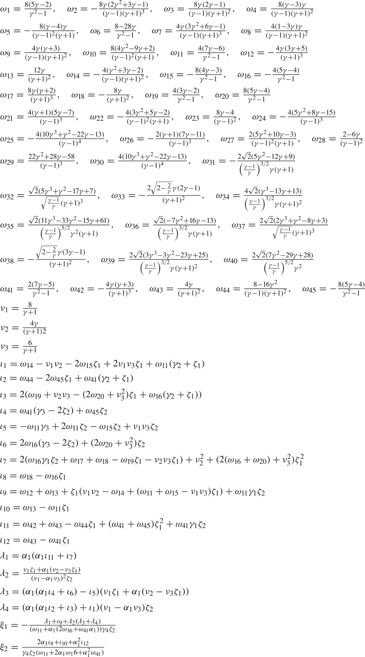
where  $\xi _1$ and
 $\xi _2$ are coefficient functions of
 $\gamma$ tabulated in table 2 in appendix A.
With initial conditions served by (4.4), (4.6), (4.11) and (4.12), evolution of the shock generated by the perturbed piston can be tracked by the GGSD systems up to second order, by integrating in time the system of equations (3.24) and (3.27) for weak and strong shocks, respectively. While, at  $t=0$, the initial values for
 $M$,
 $Q_1$ and
 $Q_2$ can be obtained faithfully from the full 2-D Euler equations, the GGSD construction does not directly propagate additional flow disturbances due to the piston motion, and carried by the
 $C^+$ characteristics when
 $t>0$. Our adoption of the GGSD theory therefore assumes that perturbations caused by the corrugated piston after the initial impulse are small and smooth; while, sufficiently far from the piston wall, the shock dynamics is mainly controlled by the intrinsic nonlinearity of its free propagation. The question of whether shock motion predicted by the GGSD systems as a function of time converge to the true solution for the Euler equations when the GGSD system order increases remains open until a direct comparison can be made.
5. Numerical results
We describe numerical simulations of the initial value problem formulated in § 4 for the specific heat ratio fixed at  $\gamma =5/3$. Spatial derivatives with respect to
 $\beta$ in the GGSD systems are discretized using a fourth-order compact finite-difference scheme (Lele Reference Lele1992), for its ability to capture travelling waves and pseudo-spectral convergence, on a uniform grid in
 $\beta$ of size
 $N=2048$. The spectral method is not used owing to large aliasing errors produced to the high-order nonlinearities in the systems. Time integration is performed with a variable time-stepping fourth-order Runge–Kutta method (RK4). All results are presented using the length unit
 $\tau =a_0 M_0 t$ for time measurement, as
 $\tau$ corresponds to the distance travelled by an unperturbed shock at any given time
 $t$.
If the shock profile remains smooth, we expect that  $M(\beta ,t)$ and
 $z(\beta ,t)$ will remain single-valued functions with bounded derivatives. We consider that a singularity has appeared at a time when an unbounded derivative in any quantity, of any order, has developed. As the systems evolve, an edge-detection algorithm (Gelb & Tadmor Reference Gelb and Tadmor2006) that searches for discontinuities on discrete data is applied on the dataset representing
 $M(\beta ,t)$. A brief outline of the algorithm is given in appendix D. Detection of an ‘edge’ in the discrete
 $M(\beta ,t)$ at some
 $t =t_c$ is interpreted to indicate the presence of an infinite
 $\partial M/\partial \beta$ corresponding to ‘overturning,’ and hence a singularity in the GGSD solution. This will generally also indicate the occurrence of curvature singularities in the shock shape
 $Z$ (Mostert et al. Reference Mostert, Pullin, Samtaney and Wheatley2017, Reference Mostert, Pullin, Samtaney and Wheatley2018a). For each set of given initial values, varying the choices of the two required tuning parameters
 $q$ and
 $J_\text {crit}$ (see (D 7) and (D 8) in appendix D) leads to less than 2 % variations in estimating
 $t_c$ compared to the reported
 $t_c$ values obtained using
 $q=1.1$ and
 $J_{crit}=1$.
For  $t>t_c$, the numerical solution for
 $M(\beta ,t)$ quickly develops rapid oscillations around the jump location. The spatial derivatives,
 $\partial M/\partial \beta$ and
 $\partial ^2 M/\partial \beta ^2$, can no longer be accurately captured by the compact finite-difference method. Proper continuation of the shock evolution for
 $t>t_c$ would require the insertion of a shock–shock into the GGSD shock-evolution description, much as is done following shock formation for the Euler equations (Eggers et al. Reference Eggers, Grava, Herrada and Pitton2017). Our present interest is evolution up to
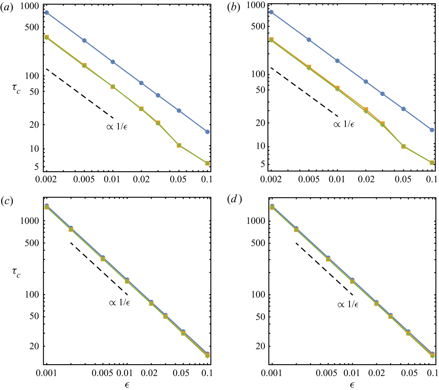
 $t=t_c$ only, and so this is not done presently. It is demonstrated subsequently that all three GGSD systems, the zeroth, first and second order, predict spontaneous development of curvature singularities on the shock shape at a finite time that is inversely proportional to the small initial perturbation size
 $\epsilon$. The critical time at which singularity occurs converges within the GGSD hierarchy as the order of systems increases.
5.1. Spontaneous singularity formation
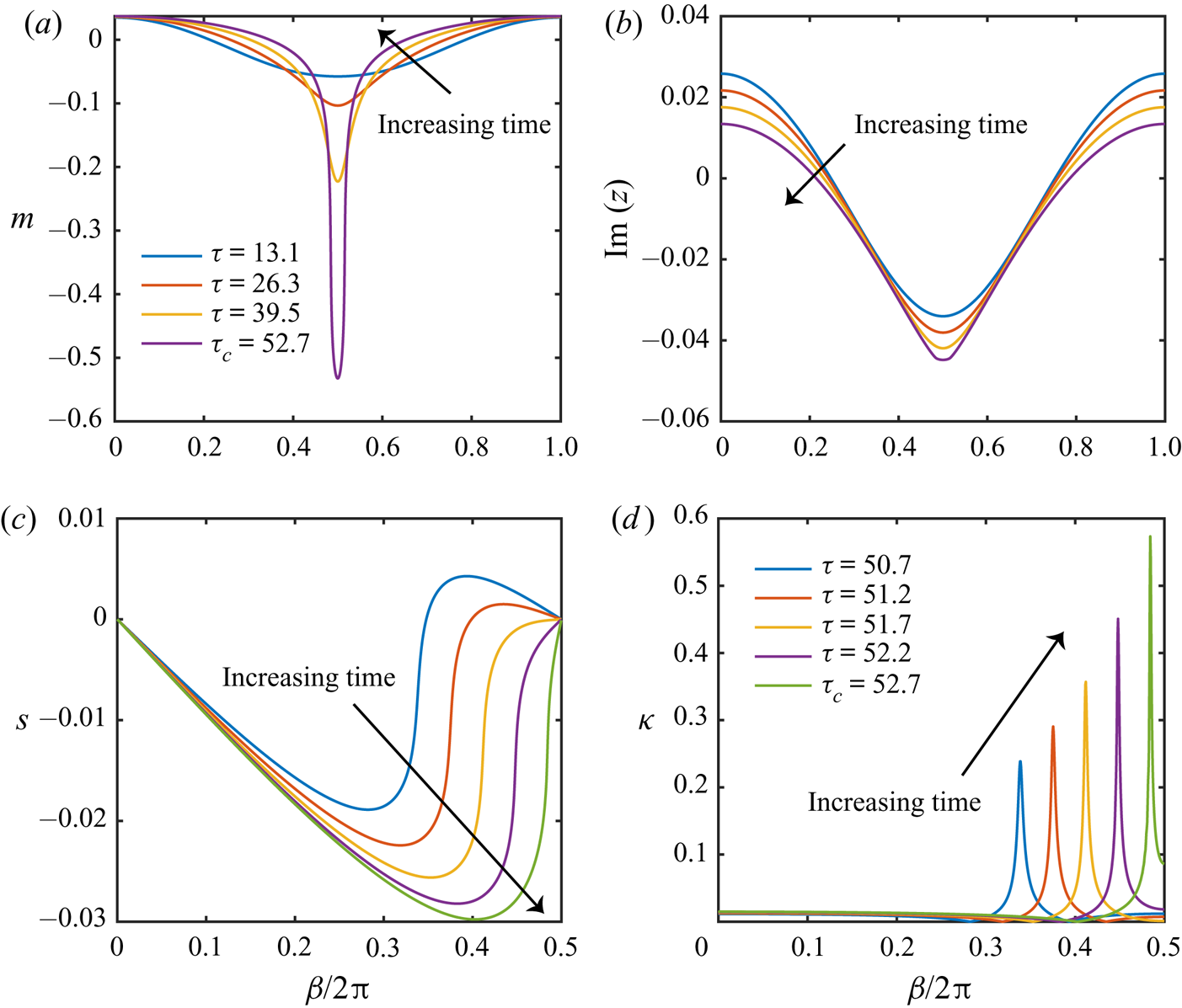
We first show the perturbation profiles of Mach number  $m$ and shock shape
 $z$ as a function of the ray-tube marker
 $\beta$ in figure 3(a) and (b), respectively, for successive times obtained using GGSD-0 with initial piston Mach number
 $M_0=50$ and perturbation amplitude
 $\epsilon =0.03$. Here, curves of different times are separated by the period of the fundamental linear mode in (3.37), i.e.
 ${\rm \Delta} \tau =1/\sqrt {\zeta _1}=13.2$, up to the critical time,
 $t_c=52.7$, when discontinuities in
 $m$ are detected by the edge-detection algorithm. As time increases, it is seen in figure 3(a) that the symmetric
 $m$ distribution steepens in each oscillation cycle, and correspondingly in figure 3(b) the normal shock displacement given by
 $\textrm {Im}(z)$ evolves towards the formation of two kinks. Because the lateral displacement
 $\textrm {Re} (z)$ is a continuous function of
 $\beta$, the observed loss of continuity in
 $m$ and smoothness in
 $z$ also occur spatially in terms of shock positions
 $Z$. In a closer look, figure 3(c) and (d) employ a smaller time interval
 ${\rm \Delta} \tau =0.5$ within one period for the same parameters
 $M_0=50$ and
 $\epsilon =0.03$ to show, leading up to the critical time, the evolution of shock slope
 $s$, calculated as
 $s=\textrm {Im}(\partial Z/\partial \beta )/\textrm {Re}(\partial Z/\partial \beta )$, and curvature
 $\kappa$, identified as
 $\kappa =\varPhi$ thanks to (2.22) and (3.13a,b). We see that, near the critical time,
 $s$ is everywhere finite but approaching a discontinuity at the point where
 $\kappa$ appears to form a singularity. These results are consistent with the findings of Mostert et al. (Reference Mostert, Pullin, Samtaney and Wheatley2018a), where the Whitham's original GSD equations are applied to a hypothetical initial value problem for a plane shock with a single Mach-number perturbation.
Spontaneous development of curvature singularities illustrated using GGSD-0 with initial conditions  $M_0=50$ and
 $\epsilon =0.03$. The Mach-number and shock-shape perturbation profiles are given over four oscillation periods up to the critical time in (a) and (b), respectively. The shock slope and curvature distributions are shown as the critical time is approached with time increments of
 ${\rm \Delta} \tau =0.5$ in (c) and (d), respectively.

Although the example given here is obtained using GGSD-0, the character of the spontaneous curvature singularity development is similarly found for GGSD-1 and GGSD-2. It is thus suggested that the ‘shock–shock’ mechanism described by Whitham (Reference Whitham2011), where nonlinear compression waves propagating along the shock, reinforcing each other to the formation of discontinuities, also holds in the present study, where a global  $A$–
 $M$ relation breaks down and non-uniform effects of the flow immediately behind the shock are accommodated.
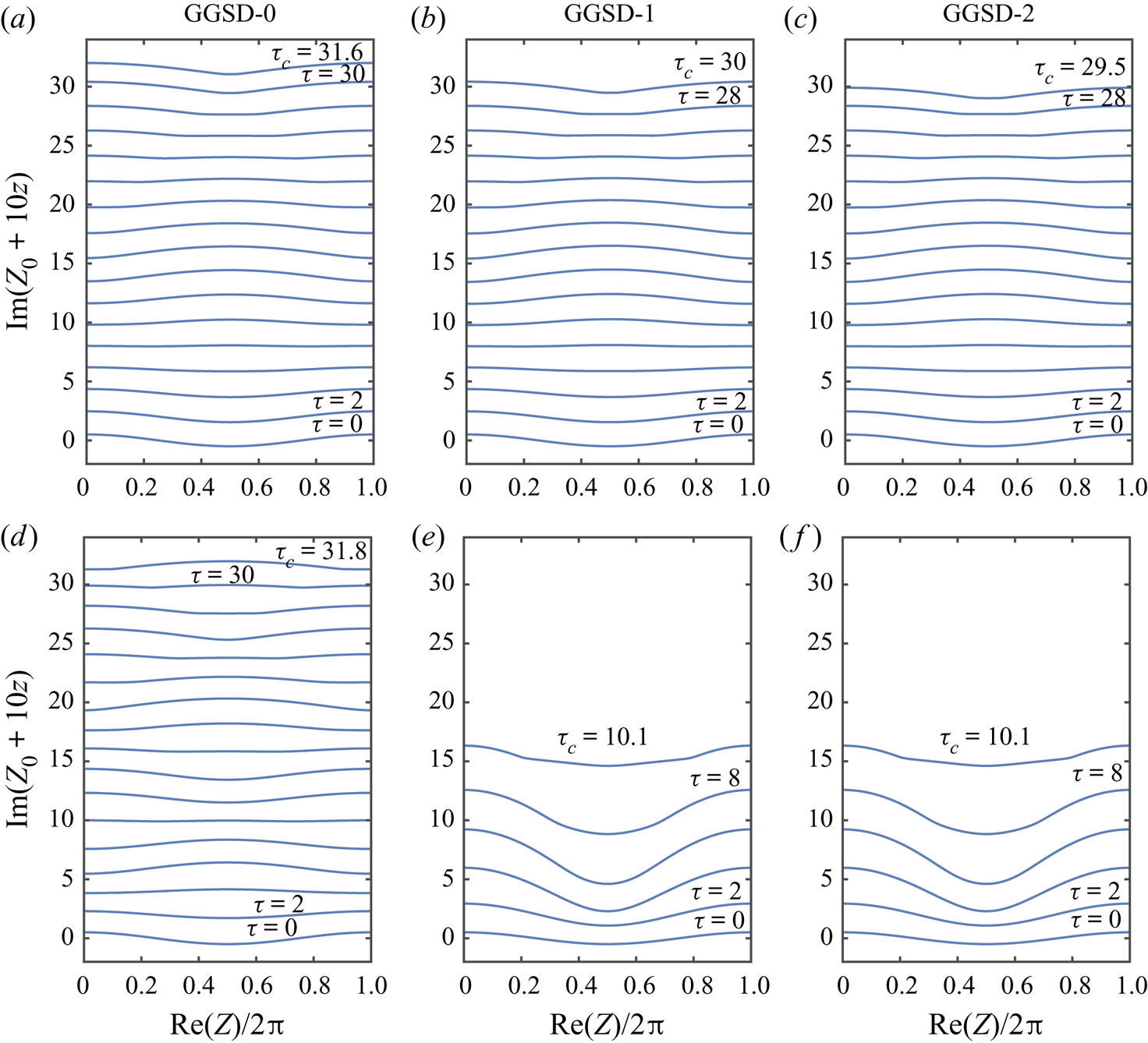
Next, typical evolving trajectories of the weak and strong shocks for  $0\leq \tau \leq \tau _c$ predicated by the three GGSD systems are presented in figure 4 for both a weak shock with
 $M_0=1.1$,
 $\epsilon =0.05$ (figure 4a–c) and a strong shock with
 $M_0=10$,
 $\epsilon =0.05$ (figure 4d–f). A transition of the amplified shock shape from its smooth initial value to a non-differentiable profile with two cusps at the critical time is observed in all cases shown. The oscillatory shock-shape pattern given by GGSD-0 is evident in both limits, with oscillation frequencies that match the linear analysis of the fundamental mode in (3.37), i.e.
 $\omega =\sqrt {\zeta _1}$ in the strong-shock limit (
 $M_0=10$) and
 $\omega =\sqrt {(M_0-1)/2}$ in the weak-shock limit (
 $M_0=1.1$). Comparing the GGSD models of different orders, differences in the detailed trajectories are small for
 $M_0=1.1$, noting that the values for
 $\tau _c$ are also close to each other. This suggests that, in the weak-shock limit, the non-uniform effect behind the shock is small and that GGSD-0 provides a good approximation.
Shock trajectories with perturbation in the  $Y$-direction amplified 10 times for piston perturbation size
 $\epsilon =0.05$. The initial piston Mach number is
 $M_0=1.1$ in (a–c) and
 $M_0=10$ in (d–f), corresponding to results obtained from the zeroth-, first- and second-order GGSD systems, respectively. In each panel, successive trajectories are shown in increments of
 ${\rm \Delta} \tau =2$, up to the final curve given at the critical time
 $\tau _c$.

In contrast, with  $M_0=10$, the first- and second-order systems predict very similar trajectories with almost the same
 $\tau _c$ that is significantly shorter than the zeroth-order value. In this case, evolution of the Mach-number perturbation
 $m$ is further investigated in figure 5 using the same parameters
 $M_0=10$ and
 $\epsilon =0.05$, where the profiles of
 $m$ along the shock are shown for the entire history of the shock trajectories. The nonlinear solution of GGSD-0 seen in figure 5(a) again shows the oscillatory pattern that is consistent with the corresponding linear theory, noting that stable oscillation in time is here terminated by the onset of discontinuities in
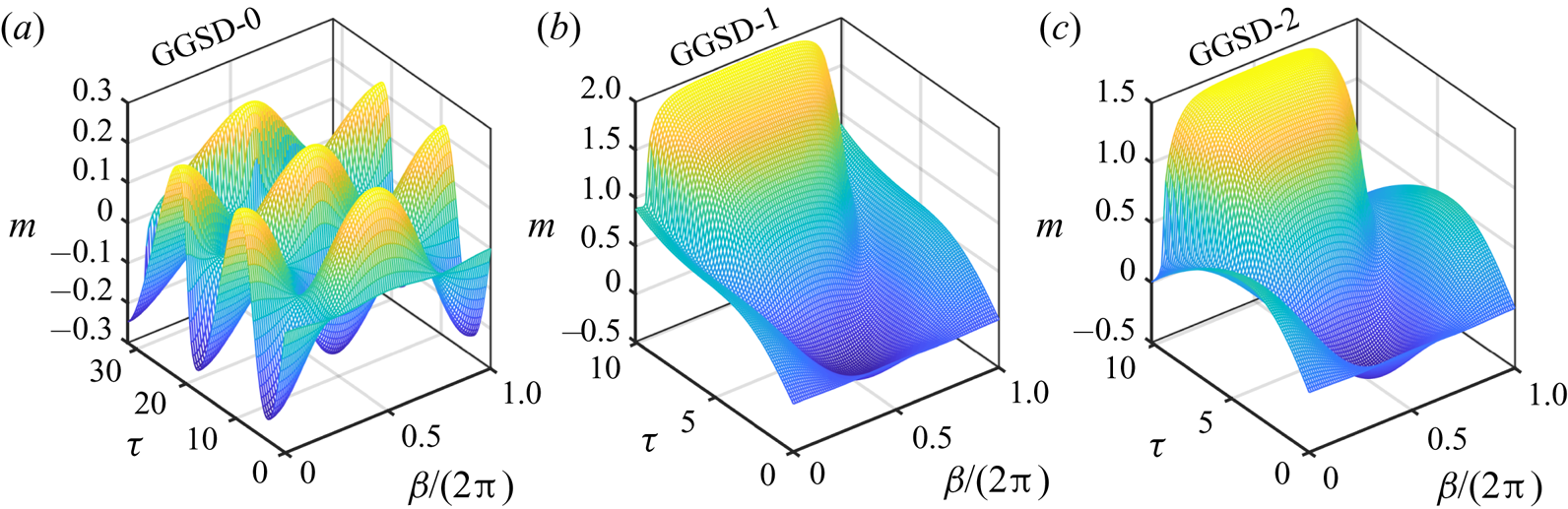
 $m$ owing to reinforcing waves on the shock. In contrast, for GGSD-1 and GGSD-2, where linear analysis predicts a growth that is linear in time, the Mach-number profiles in figure 5(b) and (c) demonstrate that the underlying osculations are dominated by approximately linear growth, until nonlinear effects accumulate, leading to
 $m$ discontinuities at the critical time. This result shows that the initial and subsequent downstream non-uniformity plays a crucial role in determining the shock motion.
History of Mach-number perturbation profile  $m$ along the evolving shock, for
 $\epsilon =0.05$ and
 $M_0=10$. Results obtained using three different orders of GGSD models are shown in (a)–(c).

5.2. Critical time
Figure 6 shows  $\tau _c$ given by the three GGSD systems as a function of the piston perturbation
 $\epsilon$, in both strong-shock (figure 6a,b) and weak-shock (figure 6c,d) limits. First, in agreement with the observation made from figure 4, the strong-shock limit sees a dramatic reduction in
 $\tau _c$ comparing GGSD-0 to the other two higher-order models, while GGSD-1 and GGSD-2 appear to have converged within the GGSD framework in terms of their
 $\tau _c$ predictions. The weak-shock limit shows much smaller differences between the three models. When at least the
 $Q_1$ correction is considered in the equations, for the cases shown here with initial Mach numbers
 $M_0=10$ and
 $M_0=50$, the decrease in
 $\tau _c$ is found to be over 50 % across all simulations with varying
 $\epsilon$. For
 $M_0=1.1$ and
 $M_0=1.02$, a decrease in
 $\tau _c$ is still consistently present, although the magnitude falls within the uncertainties of the edge-detection algorithm. On the other hand, the difference made by further including the
 $Q_2$ correction in GGSD-2 is insignificant for all
 $M_0$ simulated. These results provide convincing evidence for the convergence of the GGSD hierarchy and showcase the power of higher-order methods in handling shocks that lead to a strongly non-uniform flow, whose effect seems to increase with Mach number.
Critical times in strong- and weak-shock limits given for (a)  $M_0=10$, (b)
 $M_0=50$, (c)
 $M_0=1.1$ and (d)
 $M_0=1.02$. In all four cases, results obtained using GGSD-0 are shown as circles, GGSD-1 as squares and GGSD-2 as diamonds. In each panel, the dashed line without markers displays a reference function that has inverse power law of degree one.

An intuitive explanation of the GGSD hierarchy convergence in this application can be offered by comparing the order-of-magnitude estimates made for  $Q_1$ and
 $Q_2$ when deriving the GGSD equations, to the independently calculated initial values of
 $Q_1$ and
 $Q_2$. In §§ 3.2 and 3.3, it was shown that
 $Q_1\gtrsim O(\varepsilon _{w}^0)$ and
 $Q_2 \gtrsim O(1/\varepsilon _{w})$ as
 $\varepsilon _{w}=M-1\to 0$, and
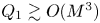 $Q_1\gtrsim O(M^3)$ and
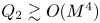 $Q_2\gtrsim O(M^4)$ as
 $M\to \infty$, in order to retain the corresponding
 $Q_1$ and
 $Q_2$ corrections in the leading-order dominant balance. Meanwhile, as
 $\epsilon \to 0$, the initial conditions for
 $Q_1$ and
 $Q_2$, obtained in § 4.3 without the GGSD truncation error, are
 $Q_1\sim \epsilon (M_0-1)$ and
 $Q_2 \sim \epsilon ^2(M_0-1)^3$ as
 $M_0\to 1$, and
 $Q_1\sim \epsilon M_0^3$ and
 $Q_2\sim \epsilon ^2M_0^4$ as
 $M_0\to \infty$. As a result, the initial condition that best matches its minimum order of magnitude required by the asymptotic GGSD equations is that of
 $Q_1$ in the strong-shock limit, where indeed the effect of
 $Q_1$ on
 $\tau _c$ is shown to be the largest.
Another finding of interest from figure 6 is that all three GGSD methods show a critical time  $\tau _c(\epsilon )$ as inversely proportional to the initial perturbation size
 $\epsilon$ for sufficiently small
 $\epsilon$, for all Mach numbers
 $M_0$. A suggested form is
 \begin{equation} \tau_c=\tau_c(\epsilon,M_0; d)=\frac{K_1(M_0;d)}{\epsilon},\quad \epsilon\ll 1, \end{equation}
where  $K_1$ is a proportionality constant that depends on
 $M_0$ and the order of the GGSD models,
 $d\in \{0,1,2\}$. The asymptotic domain of minimum
 $\epsilon$ where (5.1) applies seems to be
 $M_0$-dependent, particularly for strong shocks. Together with the similar analytic form obtained by Mostert et al. (Reference Mostert, Pullin, Samtaney and Wheatley2018a), the present results, including the established connection between the GGSD hierarchy and the Euler equations, provides compelling evidence that (5.1) is a universal form for perturbed planar shock waves.
From a computational perspective, we note that, in figure 6, the smallest  $\epsilon$ achieved in the strong-shock limit is
 $\epsilon =0.002$, doubling the value
 $\epsilon =0.001$ in the weak-shock limit. This is because an explicit time integration method such as RK4 appears to be unstable and costly for further reduction in
 $\epsilon$. An implicit method might be preferred should results for
 $\epsilon <0.002$ and
 $M\gg 1$ be desired. This is not done presently owing to the associated high cost of iteratively solving order-
 $N$ nonlinear equations at each time step.
To illustrate that the choice of  $M_0$ in figure 6 adequately represents the strong- and weak-shock limits, figure 7 plots
 $\tau _c$ for two sequences of extreme values of
 $M_0$, obtained for
 $\epsilon =0.02$ when
 $M_0\gg 1$ and for
 $\epsilon =0.01$ when
 $M_0-1\ll 1$, in all three GGSD systems. Convergence in
 $\tau _c$ is clear as
 $M_0>50$ and
 $M_0-1<0.02$ for strong and weak shocks, respectively.
Convergence of critical time (a) as  $M_0$ increases in the strong-shock limit for
 $\epsilon =0.02$, and (b) as
 $M_0$ decreases in the weak-shock limit for
 $\epsilon =0.01$. Circles, squares and diamonds correspond to GGSD-0, GGSD-1 and GGSD-2 data, respectively.

5.3. Diagnostic statistics
We have seen in figure 4 that the GGSD-1 and GGSD-2 in the strong-shock limit produce distinctly interesting shock trajectories before curvature singularities form. Figure 8 therefore presents the key statistics that characterize the evolution given by these higher-order methods up to their critical times using  $M_0=50$ and
 $\epsilon =0.02$. The mean and standard deviation of Mach-number perturbation over the shock, defined as
 \begin{equation} \bar{m}=\frac{1}{2{\rm \pi}}\int_0^{2{\rm \pi}} m\,\textrm{d}\beta \quad\mbox{and}\quad \sigma(m)=\left(\frac{1}{2{\rm \pi}}\int_0^{2{\rm \pi}} (m-\bar{m})\,\textrm{d}\beta\right)^{1/2}, \end{equation}
are shown in figure 8(a) and (b), respectively. It is observed that GGSD-0 gives an oscillating Mach-number perturbation profile around the mean, which is zero, across the profile, for all time until a discontinuity develops (critical time not shown for the dot-dashed lines in figure 8). GGSD-1 and GGSD-2 both produce on average an upward drift for  $m$ over time, where the increase is smaller with GGSD-2. This is consistent with the linear analysis in § 3.5, where (3.33) and (3.38a,b) clearly state the linear growth. Whether this mean drift will further reduce with increasing order of the GGSD systems, or if it faithfully represents the Euler equations, remains to be confirmed by direct comparisons against direct numerical simulations of the full Euler equations with high-order-accurate shock tracking. Nevertheless, despite the mean rise, the standard deviation of
 $m$ obtained from GGSD-1 and GGSD-2 shows qualitatively similar periodic fluctuations that do not grow in times, as seen in GGSD-0.
Temporal shock-profile statistics comparison between the flat (hollow circles) and perturbed shock due to three GGSD systems (different lines), made for  $M_0=50$ and
 $\epsilon =0.02$. (a,b) Mean and standard deviation of the Mach-number perturbation profile. (c) Average shock advancement in the unperturbed shock-normal direction. (d) Standard deviation of the shock-shape perturbation.

Further, as a consequence of the positive Mach-number perturbation increasing, the shock trajectories given by the higher-order methods must be accelerating at an increasingly faster rate compared to either the unperturbed flat shock or the GGSD-0 prediction. Indeed, this is reflected in figure 8(c) where the mean shock advancement,  $\textrm {Im}(\bar {Z})$, is plotted as a function of
 $\tau$. As expected from
 $\bar {m}=0$, the zeroth-order GGSD system yields a history of mean shock positions that is exactly the same as the unperturbed shock; whereas with an increasing positive
 $\bar {m}$, the mean shock position given by GGSD-1 and GGSD-2 accelerates and outruns the flat shock. Particularly, the
 $Q_2$ correction made by GGSD-2 to GGSD-1 partially negates the
 $Q_1$ correction applied by GGSD-1 to GGSD-0. Additionally, figure 8(d) shows that, although the standard deviation
 $\sigma (|z|)$, defined analogously to (5.2a,b), is significantly larger in GGSD-1 and GGSD-2 compared to GGSD-0, the shock-shape perturbations remain bounded.
The negation effect of GGSD-2 is related to the measure of immediate non-uniformity  $Q_1$ shown in figure 9, as a function of the evolving shock position in the complex plane for the same parameters
 $M_0=50$ and
 $\epsilon =0.02$. Identically zero in GGSD-0, the evolution of non-zero
 $Q_1$ in the higher-order models has been demonstrated to provide a considerable Mach-number correction. Specifically, comparing figure 9(a) and figure 9(b), the overall larger increase of
 $Q_1$ given by GGSD-1 than GGSD-2, especially the fact that when the critical time is approached
 $Q_1$ actually decreases in GGSD-2, matches the different growth rates of
 $\bar {m}$ observed in figure 8(a).
History of the non-uniformity measure  $Q_1$ behind the evolving shock as a function of shock positions in two dimensions. The panels compare results obtained for
 $M_0=50$ and
 $\epsilon =0.02$, using (a) GGSD-1 and (b) GGSD-2.

Curiously, with reference to figure 8(b), the distance gap between the mean shock positions predicted by GGSD-1 and GGSD-2 is further examined in figure 10. Denoting  ${\rm \Delta} Y$ as the lead distance, its maximum obviously occurs at the critical time of each model. The percentage of
 $\max ({\rm \Delta} Y)$ over the advancement of the reference flat shock, which also equals
 $\tau _c$ by definition, is shown in figure 10(a) as a function of
 $\epsilon$. A converging result of approximately 9.5 % for GGSD-1 and 4.5 % for GGSD-2 is found, noting that
 $\max ({\rm \Delta} Y)/\tau _c$ is overall weakly dependent on the simulated range of
 $\epsilon$. More interestingly, examining
 ${\rm \Delta} Y$ at a given time
 $\tau$ that is at most the earliest critical time among different models, i.e.
 $\tau <\min _{d\in \{0,1,2\}}(\tau _c(M_0;d))$, for instance choosing
 $\tau =\tau _c(0.03,50;2)=18.6$ as shown in figure 10(b), reveals a quadratic scaling law with respect to
 $\epsilon$, which holds for both GGSD-1 and GGSD-2, that is,
 \begin{equation} {\rm \Delta} Y|_\tau=K_2(M_0;d)\epsilon^2, \end{equation}
where again  $K_2$ is the constant multiplier that depends on
 $M_0$ and order number
 $d\in \{1,2\}$.
(a) Percentage maximum distance lead of average shock position given by GGSD-1 (circles) and GGSD-2 (squares) over the reference flat shock. (b) Distance lead of average shock position at a fixed time that is the critical time for the second-order method. In both cases,  $M_0=50$ and
 $\epsilon =0.03$, and the dashed line represents the first-order result, while the solid line gives the second-order method. The dashed line without markers in (b) shows an explicit function of quadratic power law.

In order to enable such distance lead obtained using higher-order methods over a flat shock, the flow behind the shock must gain more kinetic energy from the corrugated piston advancing than for the flat piston flow. Unlike a flat piston whose motion is given by the Heaviside function (see (4.1)), which advances at the same speed with the flow behind the shock for all  $t>0$, a corrugated piston of the same velocity continues to accelerate fluid in the local normal direction, possibly generating more kinetic energy into the flow for
 $t>0$.
6. Conclusions
We have reported numerical simulations of the evolution of a shock produced by an impulsively accelerated, two-dimensional piston with a sinusoidal surface corrugation of amplitude  $\epsilon$. First a complex-variable formulation of generalized geometrical shock dynamics, referred to as GGSD, is derived up to second order for both strong- and weak-shock limits. The resulting closed systems of partial differential equations are then solved numerically to give the evolution of the shock-shape and Mach-number distributions. An edge-detection algorithm is applied to test for the appearance of a singularity in the shock evolution profile at some critical time
 $\tau _c$. These simulations provide strong evidence supporting the hypothesis that a spontaneous curvature singularity develops in the shock shape as a prelude to the formation of triple points or Mach stems in
 $\tau _c$ inversely proportional to the amplitude of the piston corrugation.
The adoption of the GGSD hierarchy overcomes the limitations of previously used theories of geometrical shock dynamics, first by accommodating well-defined shock initial conditions for the shock generation process, which are calculated exactly for the piston-driven shock according to the Euler equations, and second by incorporating a quantitative description of non-uniform flow effects immediately behind the shock. The behaviour of weak shocks with Mach number close to unity is found to witness small changes when increasing the system order, while maintaining oscillations around the unperturbed shock up to the critical time of curvature singularity formation. For strong shocks with large Mach number, the inclusion of non-uniform flow correction  $Q_1\neq 0$ behind the shock in GGSD-1 and GGSD-2 predicts an overall shock acceleration compared to GGSD-0 where
 $Q_1=0$. The corresponding Mach-number perturbation growth is eventually terminated by the onset of the curvature singularity, which occurs in GGSD-1 and GGSD-2 at
 $\tau _c$ that converges with the GGSD order increasing, and that scales as
 $\tau _c\propto 1/\epsilon$ as in GGSD-0, albeit with a significantly smaller proportionality constant. Between the higher-order methods, GGSD-2 gives a smaller
 $Q_1$ correction effect than GGSD-1, manifested particularly in the smaller average shock acceleration relative to the unperturbed shock. This leaves uncertainty in the convergence of shock trajectories given by the GGSD expansion hierarchy, and remains to be resolved by direct numerical simulations for the Euler equations with accurate shock tracking.
Acknowledgements
This work was supported by the KAUST Office of Sponsored Research under Award No. URF/1/3418-01. The authors also thank Professor H. G. Hornung for helpful discussions.
Declaration of interests
The authors report no conflict of interest.
Appendix A. Tables of coefficients
This section lists all the coefficient functions used throughout this study in tables 1 and 2, as constant functions of the specific heat ratio  $\gamma$.
Constant coefficient functions in the GGSD systems, up to second order, in terms of the specific heat ratio γ.

Constant coefficients for the second-order partial derivatives of flow variables in the strong-shock limit, found in (B5)-(B8), and those for the initial value of Q2, found in (C1), associated with a shock driven by a corrugated piston. These coefficients are expressed in terms of other constant functions of γ listed in table 1.
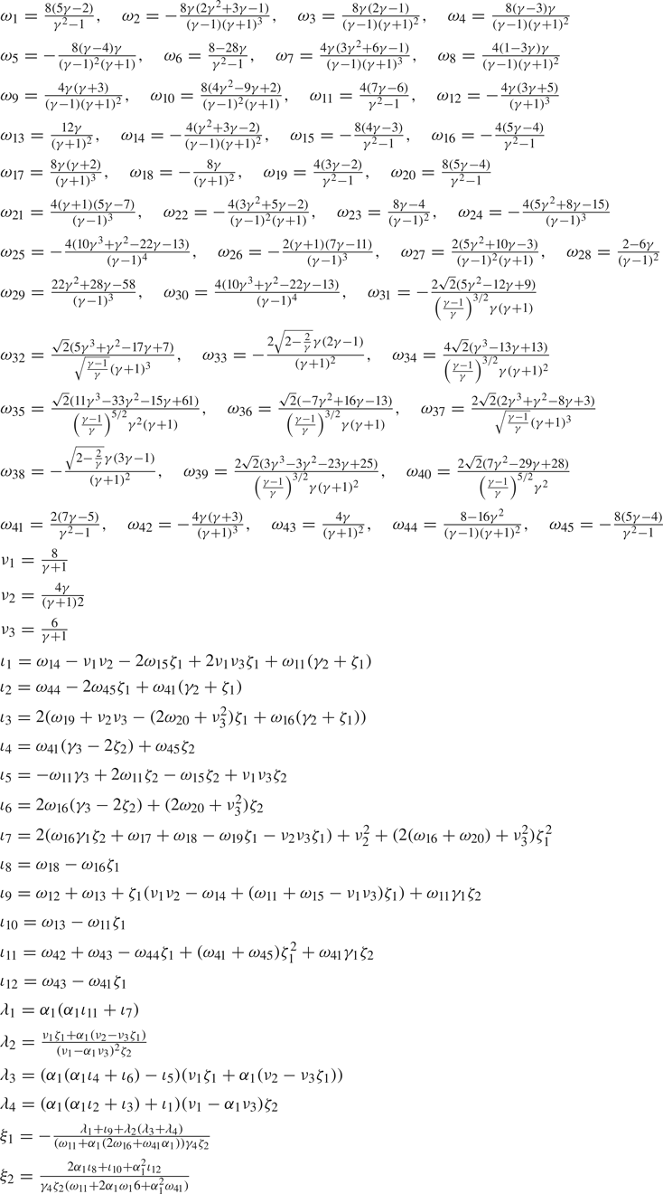
Appendix B. Partial derivatives of flow variables
The partial derivatives used in the expansions of GGSD systems are given in this section. Asymptotic expressions of the general solutions to (2.28) are obtained for both the weak- and strong-shock limits up to second order.
In the weak-shock limit where  $\varepsilon _{w}=M-1\to 0$, and in the strong-shock limit where
 $M\sim M'\to \infty$, the first-order partial derivatives are given by
 \begin{gather} \rho_t=\begin{cases} \dfrac{Q_1}{2a_0^2}+2\left[\dfrac{2Q_1}{(1+\gamma)a_0^2} +\dfrac{(\gamma-3)\rho_0a_0 \varPhi}{(1+\gamma)^2}\right] \varepsilon_{w}+O(\varepsilon_{w}^2), & \varepsilon_{w}\to 0,\\ \rho_0a_0\left[\dfrac{6 (\gamma +1)}{(\gamma -1)^2} M'+\dfrac{2}{\gamma -1} \varPhi M\right]+O(M^0), & M\to\infty, \end{cases} \end{gather}
 \begin{gather}\rho_x=\begin{cases} \dfrac{-Q_1}{2a_0^3}+\left[\dfrac{(\gamma-3)Q_1}{(1+\gamma)a_0^3} -\dfrac{4(\gamma-1)\rho_0 \varPhi}{(1+\gamma)^2}\right]\varepsilon_{w}+O(\varepsilon_{w}^2), & \varepsilon_{w}\to 0,\\ -\rho_0\left[\dfrac{6 (\gamma +1)}{(\gamma -1)^2}\dfrac{ M'}{M}+\dfrac{2}{\gamma -1} \varPhi \right]+O(M^{-1}), & M\to\infty, \end{cases} \end{gather}
 \begin{gather} u_t=\begin{cases} \dfrac{Q_1}{2\rho_0a_0}+\left[\dfrac{Q_1}{\rho_0a_0} +\dfrac{4(\gamma-1)a^2_0\varPhi}{(1+\gamma)^2}\right]\varepsilon_{w} +O(\varepsilon_{w}^2), & \varepsilon_{w}\to 0,\\ a_0^2M\left[\dfrac{8}{\gamma +1} M'+\dfrac{4 \gamma }{(\gamma +1)^2} \varPhi M\right]+O(M^1), & M\to\infty, \end{cases} \end{gather}
 \begin{gather}u_x=\begin{cases} \dfrac{-Q_1}{2\rho_0a_0^2} +\left[\dfrac{(2-6\gamma)a_0\varPhi}{(1+\gamma)^2}\right] \varepsilon_{w}+O(\varepsilon_{w}^2), & \varepsilon_{w}\to 0,\\ -a_0\left[\dfrac{6}{\gamma +1} M'+\dfrac{4 \gamma }{(\gamma +1)^2} \varPhi M\right]+O(M^0), & M\to\infty, \end{cases} \end{gather}
 \begin{gather} p_t=\begin{cases} \dfrac{Q_1}{2} +2\left[Q_1+\dfrac{(\gamma-3)\rho_0a_0^3\varPhi}{(1+\gamma)^2}\right] \varepsilon_{w}+O(\varepsilon_{w}^2), & \varepsilon_{w}\to 0,\\ \rho_0 a_0^3 M^2\left[\dfrac{4 (3 \gamma -2)}{\gamma ^2-1} M'+\dfrac{4 \gamma }{(\gamma +1)^2} \varPhi M\right]+O(M^2), & M\to\infty, \end{cases} \end{gather}
 \begin{gather}p_x=\begin{cases} \dfrac{-Q_1}{2a_0}-\left[\dfrac{Q_1}{a_0} +\dfrac{4(\gamma-1)\rho_0a^2_0\varPhi}{(1+\gamma)^2}\right]\varepsilon_{w} +O(\varepsilon_{w}^2), & \varepsilon_{w}\to 0,\\ -4\rho_0 a_0^2 M\left[\dfrac{2 \gamma -1}{\gamma ^2-1} M'+ \dfrac{\gamma }{(\gamma +1)^2}\varPhi M \right]+O(M^1), & M\to\infty, \end{cases} \end{gather}
and
 \begin{gather} a_t=\begin{cases} \dfrac{(\gamma-1)Q_1}{4\rho_0a_0}+\left[\dfrac{(\gamma-1)Q_1}{2\rho_0a_0}+ \dfrac{(\gamma-1)(\gamma-3)a_0^2\varPhi}{(1+\gamma)^2}\right]\varepsilon_{w} +O(\varepsilon_{w}^2), & \varepsilon_{w}\to 0,\\ 2a_0^2 M\sqrt{\dfrac{\gamma -1}{2 \gamma }}\left[\dfrac{ \gamma (3 \gamma -5) }{\gamma ^2-1} M'+ \dfrac{ \gamma (\gamma -1) }{(\gamma +1)^2} \varPhi M\right]+O(M^1), & M\to\infty, \end{cases}\end{gather}
 \begin{gather}a_x=\begin{cases} \dfrac{-(\gamma-1)Q_1}{4\rho_0a_0^2} -\left[\dfrac{2(\gamma-1)^2a_0\varPhi}{(1+\gamma)^2}\right] \varepsilon_{w}+O(\varepsilon_{w}^2), & \varepsilon_{w}\to 0,\\ -a_0\sqrt{\dfrac{\gamma -1}{2 \gamma }}\left[\dfrac{4 \gamma (\gamma -2) }{\gamma ^2-1} M'+ \dfrac{2 \gamma (\gamma -1) }{(\gamma +1)^2} \varPhi M\right]+O(M^0), & M\to \infty. \end{cases} \end{gather}
Similarly the limiting second-order partial derivatives as  $\varepsilon _{w}\to 0$ and
 $M\sim M'\sim M''\to \infty$ are as follows:
 \begin{gather} p_{tt}=\begin{cases} \dfrac{Q_2}{2}+O(\varepsilon_{w}^0),\\ \rho_0a_0^4M ^2[M(\omega_1 M''+(\omega_2+\omega_3)\varPhi^2M+\omega_3 \varPsi M)+ \omega_4\varPhi M M'+\omega_5M'^2]+ O(M^3), \end{cases} \end{gather}
 \begin{gather}p_{tx}=\begin{cases} -\dfrac{Q_2}{2a_0}+O(\varepsilon_{w}^0),\\ \rho_0a_0^3M [M(\omega_6M''+(\omega_7+\omega_8)\varPhi^2M+\omega_8\varPsi M )+ \omega_9\varPhi M M'+\omega_{10}M'^2 ]+O(M^2), \end{cases} \end{gather}
 \begin{gather} u_{tt}=\begin{cases} \dfrac{Q_2}{2\rho_0a_0}+O(\varepsilon_{w}^0),\\ a_0^3M [\omega_{11}M M''+M^2 ((\omega_{12}+\omega_{13})\varPhi^2+\omega_{13}\varPsi )+ \omega_{14}\varPhi MM'+\omega_{15}M'^2 ]+O(M^2), \end{cases} \end{gather}
 \begin{gather}u_{tx}=\begin{cases} -\dfrac{Q_2}{2\rho_0a_0^2}+O(\varepsilon_{w}^0),\\ a_0 ^2[\omega_{16}MM''+M^2((\omega_{17}+\omega_{18})\varPhi^2 +\omega_{18}\varPsi)+ \omega_{19}\varPhi M M'+\omega_{20}M'^2]+ O(M), \end{cases} \end{gather}
 \begin{gather}u_{xx}=\begin{cases} \dfrac{Q_2}{2\rho_0a_0^3}+O(\varepsilon_{w}^0),\\ \dfrac{a_0}{M}[\omega_{41}M M''+M^2((\omega_{42}+\omega_{43})\varPhi^2+ \omega_{43}\varPsi)+\omega_{44}\varPhi M M'+\omega_{45}M'^2]+ O(M^0), \end{cases} \end{gather}
 \begin{gather} \rho_{tt}=\begin{cases} \dfrac{Q_2}{2a_0^2}+O(\varepsilon_{w}^0),\\ \rho_0a_0 ^2[\omega_{21}M M''+M^2((\omega_{22}+\omega_{23})\varPhi^2+\omega_{23}\varPsi)+ \omega_{24}\varPhi M M'+\omega_{25}M'^2]+ O(M), \end{cases} \end{gather}
 \begin{gather}\rho_{tx}=\begin{cases} -\dfrac{Q_2}{2a_0^3}+O(\varepsilon_{w}^0),\\ \dfrac{\rho_0a_0}{M}[\omega_{26}M M''+M^2((\omega_{27}+\omega_{28})\varPhi^2+ \omega_{28}\varPsi)+\omega_{29}\varPhi M M'+\omega_{30}M'^2]+ O(M), \end{cases} \end{gather}
 \begin{gather} a_{tt}=\begin{cases} \dfrac{(\gamma-1)Q_2}{4\rho_0a_0}+O(\varepsilon_{w}^0),\\ -a_0^3M [\omega_{31}M M''+M^2 ((\omega_{32}+\omega_{33})\varPhi^2+ \omega_{33}\varPsi )+\omega_{34}\varPhi M M'+\omega_{35}M'^2 ]+O(M), \end{cases} \end{gather}
 \begin{gather}a_{tx}=\begin{cases} -\dfrac{(\gamma-1)Q_2}{4\rho_0a_0^2}+O(\varepsilon_{w}^0),\\ a_0 ^2[\omega_{36}M M''+M^2((\omega_{37}+\omega_{38})\varPhi^2+ \omega_{38}\varPsi)+\omega_{39}\varPhi M M'+\omega_{40}M'^2]+ O(M), \end{cases} \end{gather}
where  $\omega _{1,2,\ldots ,45}$ are constant functions of
 $\gamma$ given in table 2 in appendix A.
Appendix C. Derivation of the $Q_2$ initial condition

Here we provide detailed steps towards the derivation of (4.12), the initial condition of  $Q_2$ associated with the piston-generated shock.
From the kinematic condition of (4.7b), the initial jerk of flow between the piston surface and the shock is related to the initial values of partial derivatives  $u_t$,
 $u_x$,
 $u_{tt}$,
 $u_{tx}$ and
 $u_{xx}$ given in (B 1)–(B 4) and (B 5)–(B 8). Particularly, in the strong-shock limit, the
 $M'$ and
 $M''$ dependences of these derivatives can be expanded using (3.17) and (3.26) to give expressions in terms of
 $M$,
 $Q_1$,
 $Q_2$,
 $\varPhi$ and
 $\varPsi$. As a result, solving (4.7b) for
 $Q_2$ and evaluating at
 $t=0^+$ gives, for
 $M\to \infty$,
 \begin{align} Q_2(\beta,0^+) &= \left\{-\zeta _2[\varPhi(\iota_1 M^2+\iota_2 u_0^2+ \iota_3u_0 M)M^3 Q_1-(\iota_4u_0^2-\iota_5 M^2+\iota_6u_0 M)Q_1^2] \right.\nonumber\\ &\quad -M ^6[(\iota_7\varPhi^2+2\iota_8\varPsi)u_0M+(\iota_9\varPhi^2+ \iota_{10}\varPsi)M^2+(\iota_{11}\varPhi+\iota_{12}\varPsi)u_0^2] \nonumber\\ &\quad \left.+M^5\ddot{u}_0 \right\}_{t=0^+} / [\zeta_2\gamma_4M^2 (\omega_{11}M^2+ 2\omega_{16}u_0M+\omega_{41}u_0^2 )]_{t=0^+}, \end{align}
where  $\iota _{1,2,\ldots ,12}$ and
 $\omega _{11,16,41}$ are coefficients given in table 2 in appendix A. Here the initial value of
 $\varPsi$ remains to be determined. This is achieved by substituting the perturbed shock profile (4.4), together with
 $\varPhi (\beta ,0^+)$ found in (4.9), into its definition (3.22), implying that
 \begin{equation} \varPsi(\beta,0^+)=-\frac{\epsilon ^2 \sin ^2(\beta ) (\epsilon ^2 \cos (2 \beta )+2 \epsilon ^2+1)}{(\epsilon ^2 \sin ^2(\beta )+1)^3}.\end{equation}
Similarly for the weak-shock limit, expanding (4.7b) and solving for  $Q_2$ directly gives, for
 $M\to 1$,
 \begin{align} Q_2(\beta,0^+) &= \frac{2\ddot{u}_0}{(u_0-1)^2}+\left.\frac{4 (3 \gamma -1) \varPhi(M-1) +(\gamma +1)^2 Q_1}{2 (\gamma +1)^4 (u_0-1)^2}\right|_{t=0^+}\left\{(\gamma +1)^2 Q_1 \right.\nonumber\\ &\quad \left.\times (2 (M-1) -u_0+1 )+4\varPhi (M-1) [2 (\gamma-1) -(3 \gamma-1) u_0 ]\right\}_{t=0^+}. \end{align}
Now substituting (4.6), (4.8), (4.9) and (C 2) into both (C 1) and (C 3) prepares the full expression of  $Q_2(\beta ,0^+)$ in terms of the parameters
 $M_0$,
 $\epsilon$ and
 $\ddot {u}_0(\beta )$. Setting
 $\epsilon =0$ then produces
 \begin{equation} Q_2(\beta,0^+)|_{\epsilon=0}=\begin{cases} \dfrac{M_0 \ddot{u}_0}{\gamma_4\zeta_2(\omega_{11}+2\alpha_1\omega_{16}+\alpha_1^2\gamma_4)}, & M_0\to\infty,\\ \dfrac{2(\gamma+1)^2\ddot{u}_0}{(5+\gamma-4M_0)^2}, & M_0\to 1, \end{cases} \end{equation}
which must vanish as required by the unperturbed uniform flow condition. Therefore, one demands  $\ddot {u}_0=0$, suggesting that the initial flow attached to the piston has zero acceleration and jerk. Finally, for small
 $\epsilon$, (C 1) and (C 3) are Taylor-expanded to give the leading-order powers shown in (4.12):
 \begin{equation} Q_2(\beta,0^+)\sim\begin{cases} (\xi_1\cos^2(\beta)+\xi_2\sin^2(\beta) )M_0^4\epsilon^2, & M_0\to\infty,\\ -\dfrac{32 \gamma \cos ^2(\beta )(M_0-1)^3\epsilon ^2}{(\gamma +1)^3}, & M_0\to 1. \end{cases} \end{equation}
Appendix D. An edge-detection algorithm
The specific edge-detection algorithm used in § 5 that searches for the onset of a discontinuity on discrete values of the periodic function  $M(\beta ,t)$ is briefly outlined in this section. The algorithm is taken from a family of spectral methods developed by Gelb & Tadmor (Reference Gelb and Tadmor2000, Reference Gelb and Tadmor2006).
At each time step, discrete data for the Mach-number profile,  $\bar {M}_j$, subject to the rescaling
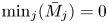 $\min _j(\bar {M}_j)=0$ and
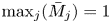 $\max _j(\bar {M}_j)=1$, is obtained first on the size
 $2N$ uniform grid
 $\beta _j=2{\rm \pi} j/(2N+1)$, where
 $j=0,1,\ldots ,2N$. The discrete concentration detector is defined as
 \begin{equation} \tilde{T}_N^c [\bar{M} ] (\beta)={\rm \pi} \textrm{i} \sum_{k=-N}^N \text{sgn}(k)\, c\left(\frac{|k|{\rm \Delta}\beta}{\rm \pi}\right)\tilde{M}_k \exp(\textrm{i}k\beta), \end{equation}
where  $\tilde {M}_k$ are the Fourier coefficients,
 \begin{equation} \tilde{M}_k=\frac{1}{2N+1}\sum_{j=0}^{2N}\bar{M}_j\exp(-\textrm{i}k\beta_j), \end{equation}
and  $c(s_k)$ with
 $s_k=|k|{\rm \Delta} \beta /{\rm \pi}$ is the concentration factor. The following two admissible concentration factors are considered next: the first-order polynomial factor,
 \begin{equation} c^{pol}(s_k)=\sin\left(\frac{{\rm \pi} s_k}{2}\right), \end{equation}
and the exponential factor,
 \begin{equation} c^{exp}(s_k)=\sin\left(\frac{{\rm \pi} s_k}{2}\right)\exp \left(\frac{1}{\alpha s_k(s_k-1)}\right)\left(\int_0^1\exp\left(\frac{1}{\alpha s(s-1)}\right)\textrm{d} s\right)^{-1}, \end{equation}
where  $\alpha =6$ is chosen (Gelb & Cates Reference Gelb and Cates2008). By invoking the minmod operator,
 \begin{equation} \text{minmod}(\,f_1,f_2)=\begin{cases} \min(\,f_1, f_2), & \text{if}\ f_1, f_2>0,\\ \max(\,f_1, f_2), & \text{if}\ f_1, f_2<0,\\ 0, & \text{otherwise}, \end{cases} \end{equation}
the two concentration factors can be combined to give
 \begin{equation} \tilde{T}_N ^{minmod}[\bar{M}](\beta) =\text{minmod} (\tilde{T}_N ^{pol}[\bar{M}](\beta),\,\tilde{T}_N ^{exp}[\bar{M}](\beta) ). \end{equation}
The concentration factors  $c$ are chosen such that all three aforementioned discrete detectors
 $\tilde {T}_N^c$ converge to the desired limit that selects jump discontinuities, i.e.
 $\lim _{\delta \to 0}[\bar {M}(\beta +\delta )-\bar {M}(\beta -\delta )]$, for all
 $\beta \in [0,2{\rm \pi} )$ as
 $N\to \infty$. The separation of scales achieved by these discrete detectors is further enhanced by the nonlinear function
 \begin{equation} E_{q,N}=N^{q/2} (\tilde{T}_N ^{minmod}[\bar{M}](\beta) )^q, \end{equation}
for some  $q>1$. This leads to the enhanced concentration method
 \begin{equation} E_N ^{minmod}[\bar{M}](\beta)=\begin{cases} \tilde{T}_N ^{minmod}[\bar{M}](\beta), & \text{if}\ |E_{q,N}|>J_{crit},\\ 0, & \text{if}\ |E_{q,N}|>J_{crit}, \end{cases} \end{equation}
where  $J_{crit}\sim O(1)$ is a global threshold below which jump discontinuities are neglected. The minmod detector is chosen here for its better performance locating discrete jumps to the nearest grid point while removing spurious oscillations.