





Introduction
The Antarctic Peninsula region is one of the most climatically dynamic sectors of Antarctica. During the second half of the twentieth century, parts of this region experienced some of the strongest atmospheric warming rates observed on the continent, although subsequent decades showed that this evolution was neither spatially uniform nor temporally monotonic (Turner et al. Reference Turner, Marshall, Clem, Colwell, Phillips and Lu2020). More recent studies have emphasized that the thermal history of the Antarctic Peninsula is better described as a sequence of warming, relative cooling or hiatus and renewed warming tendencies, with substantial spatial variability between sectors and stations (Turner et al. Reference Turner, Colwell, Marshall, Lachlan-Cope, Carleton and Jones2005, Reference Turner, Marshall, Clem, Colwell, Phillips and Lu2020, Oliva et al. Reference Oliva, Navarro, Hrbáček, Hernández, Nývlt and Pereira2017, Carrasco et al. Reference Carrasco, Bozkurt and Cordero2021, IPCC 2023). Gonzalez & Fortuny (Reference Gonzalez and Fortuny2018) further showed that temperature trends in the Antarctic Peninsula are strongly dependent on the time interval considered, with alternating warming and cooling tendencies over shorter periods, whereas the long-term warming signal becomes robust over longer time spans.
This climatic complexity is especially relevant in the South Shetland Islands, where many ice-free areas lie close to the climatic threshold of permafrost occurrence (Vieira et al. Reference Vieira, Bockheim, Guglielmin, Balks, Abramov and Boelhouwers2010, Bockheim et al. Reference Bockheim, Vieira, Ramos, López-Martínez, Serrano and Guglielmin2013, Obu et al. Reference Obu, Westermann, Vieira, Abramov, Balks and Bartsch2020, Hrbáček et al. Reference Hrbáček, Oliva, Hansen, Balks, O’Neill and de Pablo2023). In these Maritime Antarctic environments, relatively small atmospheric changes may have disproportionate consequences for active-layer thickness, snow persistence, hydrology, ecosystem functioning and the long-term stability of frozen ground. Previous regional and continental studies have shown that permafrost in Antarctic coastal and island environments is comparatively warm, spatially heterogeneous and therefore particularly sensitive to atmospheric forcing, while Antarctic permafrost as a whole is already undergoing measurable warming (Bockheim et al. Reference Bockheim, Vieira, Ramos, López-Martínez, Serrano and Guglielmin2013, Biskaborn et al. Reference Biskaborn, Smith, Noetzli, Matthes, Vieira and Streletskiy2019, Obu et al. Reference Obu, Westermann, Vieira, Abramov, Balks and Bartsch2020, Hrbáček et al. Reference Hrbáček, Oliva, Hansen, Balks, O’Neill and de Pablo2023).
Despite this relevance, most atmospheric analyses from the Antarctic Peninsula and the South Shetland Islands have focused on mean annual or seasonal temperature evolution, linear trends or the occurrence of warm and cold extremes (e.g. Kejna et al. Reference Kejna, Araźny and Sobota2013, Bello et al. Reference Bello, Suarez and Lavado-Casimiro2022, González-Herrero et al. Reference González-Herrero, González-Espejo, Jiménez-Cavero, Albero-Molina, Bañon and Aguilar-Pérez2026). These approaches are essential, but they do not explicitly separate the observed temperature signal into its recurrent seasonal structure, its low-frequency background evolution and its short-term irregular departures. As a result, they are less suited to answering how much of the variability is associated with the expected annual cycle, how much reflects a sustained shift in the thermal baseline and how much corresponds to anomalous episodes superimposed on both.
Additive time series decomposition offers a useful framework for addressing this problem because it partitions the observed series into seasonal, trend and remainder components (Cleveland et al. Reference Cleveland, Cleveland, McRae and Terpenning1990, Hyndman & Athanasopoulos Reference Hyndman and Athanasopoulos2021). In the specific case of seasonal-trend decomposition using locally estimated scatterplot smoothing (LOESS; ‘STL’ from here), the decomposition is performed through iterative locally weighted regression, which makes the method flexible, robust and suitable for non-stationary environmental series (Cleveland et al. Reference Cleveland, Cleveland, McRae and Terpenning1990). STL has become widely used because it does not require a rigid parametric formulation of the trend, it can accommodate different seasonal periods and it allows the seasonal component to remain fixed or to vary smoothly through time depending on the chosen settings (Cleveland et al. Reference Cleveland, Cleveland, McRae and Terpenning1990, Dokumentov & Hyndman Reference Dokumentov and Hyndman2015). In its stlplus implementation, the method is further extended to handle missing values directly and to provide additional smoothing and diagnostic options, which is particularly useful for long environmental monitoring series affected by observational gaps (Hafen Reference Hafen2016).
This methodological framework is well suited to air temperature data because such series typically contain three superimposed forms of variability: a strong annual cycle, a lower-frequency background evolution and short-lived irregular departures (Cleveland et al. Reference Cleveland, Cleveland, McRae and Terpenning1990, Moreno-Carbonell et al. Reference Moreno-Carbonell, Sánchez-Úbeda and Muñoz2020). For daily outdoor air temperature records, decomposition has been used to isolate long-term thermal change from recurring seasonality and from the residual term, which often contains cold and heat-wave behaviour or other anomalous short-term departures (Moreno-Carbonell et al. Reference Moreno-Carbonell, Sánchez-Úbeda and Muñoz2020). In remotely sensed land surface temperature series, decomposition has also proved useful for separating long-term climatic change from seasonal variations and short-term noise, allowing clearer interpretation of both the trend and anomaly structure (e.g. Quan et al. Reference Quan, Zhan, Chen, Wang and Wang2016). These studies are not directly Antarctic, but they demonstrate that decomposition is particularly informative when the objective is not only to describe whether temperatures are changing, but also to understand how that change is organized in time.
Within Antarctica, STL-type decomposition has already been applied to various thermal datasets, although its use for the comparative analysis of near-surface air temperature observations across a spatially compact station network remains less common. Carter et al. (Reference Carter, Leeson, Orr, Kittel and van Wessem2022) applied STL to monthly Antarctic fields of snowfall, near-surface air temperature and melt in regional climate models and reanalysis datasets, showing that seasonal, trend and residual components can be compared meaningfully across products. Kwok et al. (Reference Kwok, Qian and Kuleshov2023), working with Antarctic temperature time series containing missing data, showed that seasonal-trend decomposition based on LOESS can recover meaningful long-term structure even in incomplete records, although the accuracy depends on the smoothness of the underlying trend and the distribution of the gaps. STL has also been applied to daily soil temperature series in Maritime Antarctica, as shown by Schaefer et al. (Reference Schaefer, Francelino, Pereira, Michel, Schmitz and Sacramento2023), who decomposed thermal records at several depths in a Cryosol on Half Moon Island into seasonal, trend and remainder components. More recently, Luengo-S et al. (Reference Luengo-S, Rosado, Jiménez-Morales, de Gil, Gómez-Enri, Bruno and Berrocoso2025) applied STL decomposition to seawater temperature records from oceanographic stations on Livingston and Deception islands, providing an additional regional example of the application of this method to Antarctic environmental thermal series. In addition, LOESS-based analysis has previously been applied to near-surface air temperature records from stations included in the present network. Recondo et al. (Reference Recondo, Corbea-Pérez, Peón, Pendás, Ramos and Calleja2022) analysed daily mean air temperature at Incinerador, Collado Ramos and Reina Sofía stations on Hurd Peninsula to represent their temporal variation, although their study did not perform a full STL decomposition into seasonal, low-frequency and remainder components. Together, these studies show that STL and LOESS are established approaches that have already been applied to Antarctic environmental temperature records, including air temperature observations and thermal series from the study region. However, the comparative application of full STL decomposition to daily and monthly near-surface air temperature observations across a compact Maritime Antarctic station network, with particular attention to spatial contrasts among seasonal, low-frequency and remainder components, remains underexplored.
This gap is important because near-surface air temperature records from Livingston and Deception islands offer an opportunity to examine not only whether air temperature has changed (de Pablo & Goyanes Reference de Pablo and Goyanes2026), but also how the signal is structured across a network that includes contrasting local environments. The eight stations considered here span two islands (de Pablo Reference de Pablo2025), distinct geomorphological settings and a marked altitudinal range. They therefore provide an appropriate framework for testing whether the thermal signal is organized similarly across the network or whether its seasonal, trend and residual components vary according to local controls such as elevation, exposure and island setting. In particular, decomposition may help identify which stations are most strongly structured by the annual cycle, which show the clearest background evolution, and whether short-term warm and cold anomalies are regionally coherent or mainly local in expression.
Against this background, the aim of this study is to characterize the temporal structure of near-surface air temperature series from Livingston and Deception islands by means of additive decomposition into seasonal, trend and residual components, and to assess the spatial and climatic significance of those components across a Maritime Antarctic monitoring network. Specifically, the study addresses three questions: 1) How is the temporal variability of near-surface air temperature partitioned into seasonal, trend and residual components? 2) To what extent does the contribution of those components differ among stations with contrasting elevation, exposure and island settings? And 3) does the residual component contain coherent warm and cold anomalies that reveal regionally shared events and locally modulated responses? By addressing these questions, the study seeks to complement more conventional Antarctic temperature analyses based on trends and extremes and to provide a more explicit picture of how recent atmospheric change is organized in time in one of the most climatically sensitive sectors of Antarctica.
Materials and methods
Study area
This study focuses on eight stations of the PERMATHERMAL monitoring network (Fig. 1 & Table I) located on Livingston and Deception islands in the South Shetland Islands of the north-western Antarctic Peninsula (de Pablo Reference de Pablo2025). Six stations are situated on the ice-free terrain of Hurd Peninsula, Livingston Island, where they define a short but marked altitudinal transect from low coastal environments close to sea level to colder and more elevated sectors inland. A seventh station is located at Limnopolar Lake (LL) on Byers Peninsula, also on Livingston Island, and an eighth station is situated at Crater Lake (CL) on Deception Island. Together, these sites provide a compact but environmentally diverse network that captures contrasts in altitude, topographic exposure, maritime influence and geological setting across some of the main ice-free environments of the region (Vieira et al. Reference Vieira, Bockheim, Guglielmin, Balks, Abramov and Boelhouwers2010, Ferreira et al. Reference Ferreira, Vieira, Ramos and Nieuwendam2017, de Pablo et al. Reference de Pablo, Ramos, Vieira, Molina, Ramos and Maior2024, Reference de Pablo, Ramos, Vieira, Molina and Ruiz-Fernández2025).
Location of the eight PERMATHERMAL near-surface air temperature stations in the South Shetland Islands, Maritime Antarctica. The upper panel shows the regional setting of Livingston and Deception islands within the South Shetland Islands, including the positions of Limnopolar Lake (LL) on Byers Peninsula and Crater Lake (CL) on Deception Island, together with an inset locating the study area within Antarctica. The lower panel shows the detailed topographic setting of Hurd Peninsula, Livingston Island, where the six-station altitudinal transect is located: Juan Carlos I (JC), Nuevo Incinerador (NI), Incinerador (IN), Collado Ramos (CR), Morrena (MO) and Sofía (SO). m a.s.l. = metres above sea level.

Figure 1. Long description
The upper panel is a regional map of the South Shetland Archipelago between 61 degrees West and 58 degrees West. An inset globe of Antarctica shows the study area's location at the northern tip of the Antarctic Peninsula. On the main regional map, Livingston Island is in the West and Deception Island is to the South. Two stations are marked with black dots: L L on Byers Peninsula and C L on Deception Island. The Hoces sea lies to the North and Bransfield strait to the South.
The lower panel is a high-resolution topographic contour map of Hurd Peninsula, connected by an arrow to a circled area on Livingston Island. A scale bar indicates 200 meters. The elevation is color-coded from blue at 0 meters to red at 300 meters above sea level. Six stations are marked with black dots along an altitudinal transect:
* J C is located near the northern coast in a low-elevation blue zone.
* N I and I N are situated slightly further inland and higher in elevation.
* C R is located to the Southwest in a green mid-elevation zone.
* M O is located to the Southeast in a green mid-elevation zone.
* S O is the highest station, located on a southern peak shown in orange and red, exceeding 200 meters above sea level.
Main characteristics of the eight PERMATHERMAL near-surface air temperature stations used in this study, including location, elevation, temporal coverage and data availability over the 2000–2022 study period (see text for station name abbreviation expansions).

Table I. Long description
The table consists of eight columns: Island, Station code, Latitude, Longitude, Elevation in m a s l, Wind exposure, First record, and Data percentage.
* Livingston Island stations:
- J C: 62 degrees 39 minutes 48.815 seconds S, 60 degrees 23 minutes 26.484 seconds W, 10 m, Low exposure, 24 February 2000, 83.50 percent.
- N I: 62 degrees 39 minutes 50.744 seconds S, 60 degrees 23 minutes 09.061 seconds W, 19 m, Very low exposure, 13 February 2007, 80.91 percent.
- I N: 62 degrees 39 minutes 52.980 seconds S, 60 degrees 23 minutes 08.079 seconds W, 34 m, Low exposure, 30 January 2008, 94.95 percent.
- C R: 62 degrees 40 minutes 03.063 seconds S, 60 degrees 23 minutes 31.504 seconds W, 117 m, High exposure, 2 February 2006, 85.74 percent.
- M O: 62 degrees 40 minutes 01.671 seconds S, 60 degrees 22 minutes 31.430 seconds W, 145 m, High exposure, 9 February 2000, 60.62 percent.
- S O: 62 degrees 40 minutes 15.657 seconds S, 60 degrees 22 minutes 46.468 seconds W, 274 m, Very high exposure, 24 February 2000, 76.07 percent.
- L L: 62 degrees 38 minutes 59.100 seconds S, 61 degrees 06 minutes 16.900 seconds W, 85 m, High exposure, 12 February 2009, 92.07 percent.
* Deception Island station:
- C L: 62 degrees 59 minutes 06.845 seconds S, 60 degrees 40 minutes 45.225 seconds W, 80 m, Very high exposure, 31 January 2009, 83.78 percent.
m a.s.l. = metres above sea level.
The Livingston sites represent two distinct local contexts. The Hurd Peninsula stations (Juan Carlos I (JC), Nuevo Incinerador (NI), Incinerador (IN), Collado Ramos (CR), Morrena (MO), Sofía (SO)) are arranged along a topographic gradient that makes it possible to examine how air temperature changes with elevation, but also how it responds to differences in local relief, proximity to the coast and exposure to prevailing winds. By contrast, LL on Byers Peninsula represents a more open setting, geomorphologically different from Hurd Peninsula and influenced by different patterns of snow accumulation and wind redistribution (e.g. Bañon et al. 2013, Fassnacht et al. Reference Fassnacht, López-Moreno, Toro and Hultstrand2013, Bañon & Vasallo Reference Bañón and Vasallo2015, de Pablo et al. Reference de Pablo, Ramos and Molina2017). The network therefore does not simply sample a lapse-rate gradient but rather a set of contrasting station environments within Maritime Antarctica.
CL on Deception Island introduces a further source of contrast. Deception Island is an active volcanic island with a flooded caldera and widespread pyroclastic and volcanic deposits, and therefore it differs substantially from the Livingston Island sites in substrate, local topography and geothermal context (e.g. Goyanes et al. Reference Goyanes, Vieira, Caselli, Cardoso, Marmy and Santos2014). These differences are potentially relevant because local atmospheric conditions at this station may be influenced not only by regional climate, but also by volcanic terrain and sheltering effects. At the regional scale, both Livingston and Deception islands belong to the Maritime Antarctic domain (Bañon & Vasallo Reference Bañón and Vasallo2015, González-Herrero et al. Reference González-Herrero, González-Espejo, Jiménez-Cavero, Albero-Molina, Bañon and Aguilar-Pérez2026), where mean annual air temperature is commonly close to the climatic threshold of permafrost occurrence. In such settings, relatively small atmospheric changes may have disproportionate consequences for frozen-ground conditions (Bockheim et al. Reference Bockheim, Vieira, Ramos, López-Martínez, Serrano and Guglielmin2013, Obu et al. Reference Obu, Westermann, Vieira, Abramov, Balks and Bartsch2020, de Pablo et al. Reference de Pablo2025, de Pablo & Goyanes Reference de Pablo and Goyanes2026).
The monitored sites range from 10 to 274 m above sea level (a.s.l.; Table I) and include JC (10 m), NI (19 m), IN (34 m), CR (117 m), MO (145 m), SO (274 m), LL (85 m) and CL (80 m). This spatial configuration makes it possible to compare both island-scale and station-scale differences in the temporal behaviour of near-surface air temperature.
Air temperature data
The analysis uses near-surface air temperature records from the eight PERMATHERMAL stations for the period 1 January 2000–31 December 2022 (Table I). Air temperature was measured at 1.60 m above the ground surface on vertical masts using Gemini TinyTag Plus 2 data loggers connected to PT100 external temperature probes, ± 0.1°C in resolution (Gemini Data Loggers 2018), housed in radiation shields. In the network configuration considered here, the sensors were operated at hourly resolution, and data were retrieved during annual field campaigns (de Pablo Reference de Pablo2025, de Pablo et al. Reference de Pablo, Bermejo, Goyanes and Sánchez2026).
The temporal coverage of the stations (Fig. 2 & Table I) is uneven because the network was progressively established and because some records contain gaps caused by battery depletion, logger or probe malfunction, mast damage or logistic constraints affecting annual maintenance and data recovery. The longest records extend back to 2000, whereas others begin later, especially at LL and CL. Data coverage is generally higher than 80%, except for MO (~60%) and SO (~75%) stations. Higher coverage (IN station) reaches ~95%. In any case, no gap-filling was applied, and all analyses were therefore based exclusively on directly observed records, and temporal continuity was evaluated explicitly before subsequent aggregation and decomposition steps. This conservative approach was adopted to avoid introducing artificial variability or suppressing short-term anomalies that may themselves be climatically meaningful.
Annual availability of valid daily near-surface air temperature data for the eight PERMATHERMAL stations during 2000–2022 (see text for station name abbreviation expansions). Shading intensity represents the percentage of valid daily observations available for each station and year.
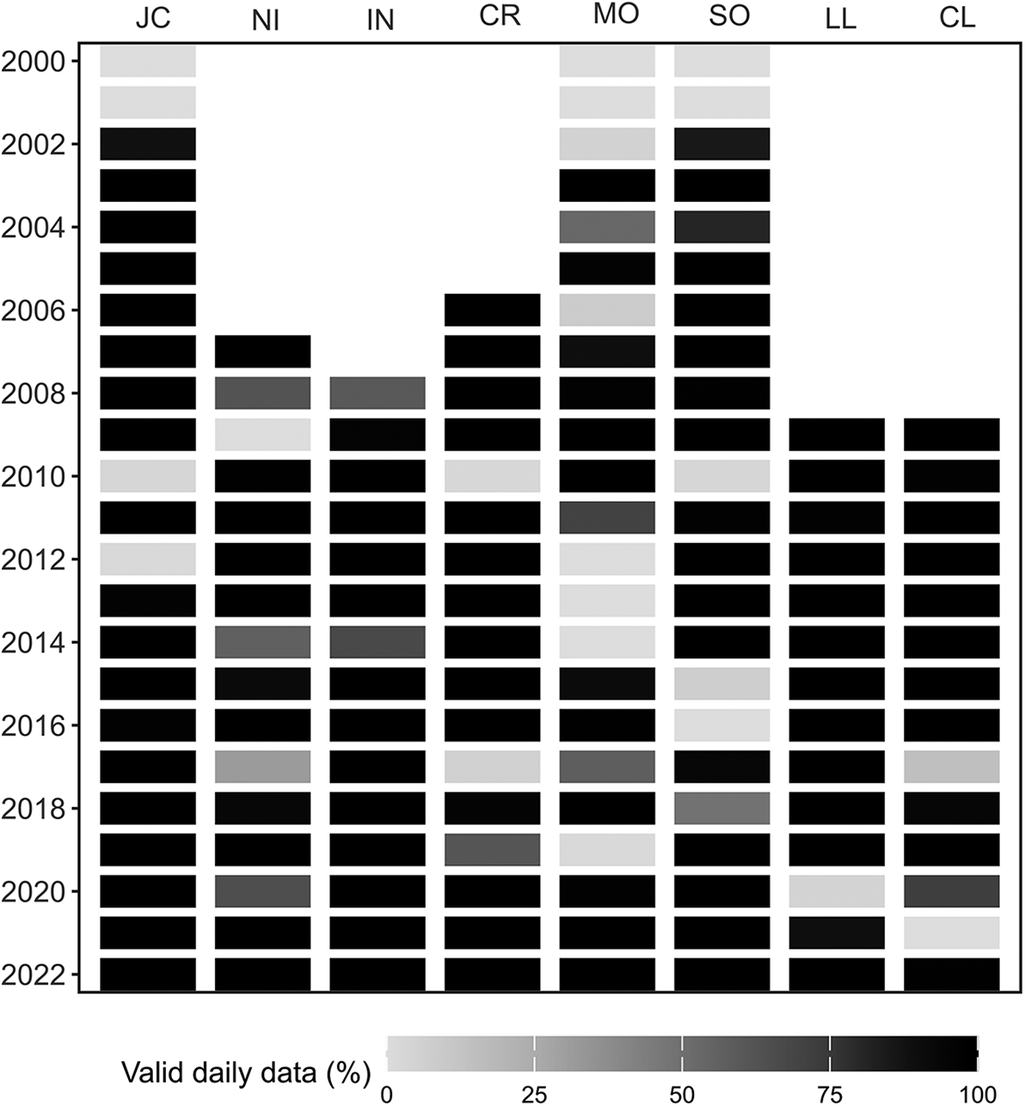
Figure 2. Long description
A heatmap grid with eight vertical columns representing stations and 23 horizontal rows representing years from 2000 to 2022.
* Axes and Legend: The X-axis at the top lists station initialisms: J C, N I, I N, C R, M O, S O, L L, and C L. The Y-axis on the left lists years in increments of two. A legend at the bottom titled Valid daily data (%) shows a grayscale gradient from white (0) to black (100).
* Data Distribution by Station:
- J C: Data begins in 2000 with low availability (light gray), becoming consistently high (black) from 2002 onwards, with occasional dips to light gray in 2010 and 2012.
- N I: Data collection starts in 2007. It shows high availability (black) for most years, with moderate gray shading in 2008, 2014, 2017, and 2020.
- I N: Data collection starts in 2008. It maintains high availability (black) through 2022, with a single moderate gray dip in 2014.
- C R: Data collection starts in 2006. It shows high availability (black) with light gray gaps in 2010 and 2017, and dark gray in 2019.
- M O: Data exists from 2000. It is highly fragmented with frequent light gray (low availability) and dark gray (moderate availability) blocks interspersed with black blocks.
- S O: Data exists from 2000. It shows high availability (black) from 2002 to 2022, with light gray gaps in 2010 and 2015.
- L L and C L: Both stations begin data collection in 2009. Both show predominantly high availability (black) through 2022, with L L having a light gray gap in 2020 and C L having light gray gaps in 2017 and 2021.
The present study was designed as an internally comparative analysis of the temporal structure of the PERMATHERMAL series. Although official meteorological observations are available for Livingston and Deception islands (González-Herrero et al. Reference González-Herrero, González-Espejo, Jiménez-Cavero, Albero-Molina, Bañon and Aguilar-Pérez2026), the PERMATHERMAL records have not yet been systematically cross-validated against those reference observations. Accordingly, the results presented here are intended to characterize relative temporal and spatial patterns within the PERMATHERMAL network and should not be interpreted as directly validated equivalents of results derived from standard meteorological stations.
Data processing and aggregation
All data preparation, decomposition and graphical analyses were performed in R using custom scripts developed for this study and run in RStudio (R Core Team 2025, Posit Team Reference Team2025). The workflow was designed to process all station files in batch mode, aggregate the hourly observations to daily and monthly series and generate directly comparable outputs for each station and for the network as a whole. The implementation relied mainly on the packages lubridate (Grolemund & Wickham Reference Grolemund and Wickham2011), dplyr (Wickham et al. Reference Wickham, François, Henry, Müller and Vaughan2026), tidyr (Wickham et al. Reference Wickham, Vaughan and Girlich2025), ggplot2 (Wickham Reference Wickham2016), rstudioapi (Ushey et al. Reference Ushey, Allaire, Wickham and Ritchie2026) and stlplus (Hafen Reference Hafen2016).
A day was considered valid when at least 75% of the expected hourly observations were available, equivalent to 18 of 24 records. A month was considered valid when at least 80% of the expected daily values were present. Daily values were calculated as the arithmetic mean of the valid hourly observations, and monthly values were calculated as the mean of the valid daily series. These thresholds were chosen to maintain consistency with previous analyses of the PERMATHERMAL air temperature series (de Pablo & Goyanes Reference de Pablo and Goyanes2026) and to ensure that the decomposed series retained a minimum level of observational representativeness while preserving real data gaps. The 75% daily data threshold also limits the potential influence of incomplete sub-daily coverage on calculated daily means by requiring observations across most of each daily cycle. Although systematic losses concentrated in particular hours could potentially bias daily means, their effect is expected to be limited in these Maritime Antarctic stations, where diurnal air temperature ranges are generally small; the same daily validity threshold has also recently been applied to nearby official atmospheric records (González-Herrero et al. Reference González-Herrero, González-Espejo, Jiménez-Cavero, Albero-Molina, Bañon and Aguilar-Pérez2026).
For the daily decomposition, 29 February was removed in leap years so that the annual cycle could be represented with a constant periodicity of 365 days. Monthly decompositions were performed with a periodicity of 12 months. The purpose of this aggregation was not to suppress variability but to distinguish between two complementary analytical scales: a daily scale that preserves short-term thermal anomalies and a monthly scale that more clearly resolves the annual seasonal structure and the background temporal evolution.
Additive temporal decomposition
To characterize the internal temporal structure of the air temperature series, assuming it is a stochastic process, we applied an additive STL, following the general framework introduced by Cleveland et al. (Reference Cleveland, Cleveland, McRae and Terpenning1990). In additive form, the observed series yt was represented as in Equation 1:

where Tt is the trend component, St is the seasonal component and Rt is the remainder or irregular component at time t (Cleveland et al. Reference Cleveland, Cleveland, McRae and Terpenning1990).
The decomposition was implemented with the stlplus package, which extends the original STL framework by allowing missing values and additional smoothing and diagnostic options while preserving the same seasonal-trend-remainder structure as the original method (Hafen Reference Hafen2016). STL was selected because it is well suited to environmental time series with strong seasonality and because its LOESS-based structure makes it possible to separate the recurrent annual thermal cycle from the low-frequency background evolution and the short-term residual variability without imposing a rigid parametric model.
For the present analysis, the daily series were decomposed using an annual seasonal period of 365 days and the monthly series were decomposed using a period of 12 months. The decomposition also required specification of the seasonal window type, the trend window and the robustness settings. The seasonal window determines whether the annual cycle is treated as fixed or allowed to vary smoothly through time, the trend window controls the degree of smoothing applied to the trend component and the robustness settings regulate the influence of anomalous observations on the decomposition. The final selection of these parameters was based on the sensitivity analysis described earlier and presented in more detail later.
Quantification of the decomposition components
For each station and each decomposition, several summary metrics were extracted from the seasonal, trend and remainder components. These included the standard deviation of each component, the mean and range of seasonal amplitude, the initial and final values of the trend component and its endpoint difference (ΔTt ), calculated from the first and last estimated Tt values available for each station and normalized to a 10 year interval. ΔTt is a descriptive endpoint-change metric for the smoothed trend component over the particular observation period covered by each station; it is not a linear trend estimate or a regional atmospheric warming rate, and it may be influenced by the thermal conditions occurring near the beginning and end of each record. To quantify the relative importance of the seasonal and trend components, we calculated the strength of seasonality (FS ) and the strength of trend (FT ) using the variance-ratio metrics proposed by Wang et al. (Reference Wang, Smith and Hyndman2006), as presenting in Equations 2 & 3:


where St is the seasonal component, Tt is the trend component and Rt is the remainder (or irregular) component of the decomposed air temperature series at time t. Because the original series is expressed in degrees Celsius, the three components St , Tt and Rt are also expressed in degrees Celsius.
Accordingly, Var denotes the statistical variance of each component, with units of °C2. By contrast, FS and FT are dimensionless indices, ranging theoretically from 0 to 1, and therefore have no physical units. Higher values of FS indicate that the variability of the series is more strongly controlled by the recurring seasonal cycle, whereas higher values of FT indicate a greater contribution of the long-term trend relative to the residual variability. In practical terms, a high FS indicates a strongly recurrent annual thermal cycle, whereas a high FT indicates that a substantial part of the variability is associated with low-frequency temporal change rather than short-term irregular fluctuations. These indices therefore provide a compact way to compare the relative importance of seasonality and background temporal evolution among stations (Wang et al. Reference Wang, Smith and Hyndman2006).
For the remainder component, we calculated the standard deviation, interquartile range, lower and upper percentiles, skewness and kurtosis. These descriptors were used to assess the magnitude, asymmetry and extremeness of residual variability after removing both the expected seasonal cycle and the background trend. Annual and seasonal summaries of the remainder were also calculated to identify years or seasons with anomalously high residual variability.
Residual event detection
The Rt component represents short-term departures not captured by the estimated seasonal and trend components. However, because the remainder may also include observational noise, unresolved seasonal structure and decomposition-related effects, it was used here to identify candidate warm and cold residual events rather than to attribute a physical meteorological cause to those departures. Event detection required specification of two parameters: a magnitude threshold, defined in terms of station-specific percentiles of the daily remainder distribution, and a minimum event duration, defined as the minimum number of consecutive days exceeding that threshold. In this framework, warm residual events were identified from positive exceedances above an upper percentile threshold, whereas cold residual events were defined analogously from negative exceedances below a lower percentile threshold. These parameters were evaluated through the sensitivity analysis described earlier and presented in more detail later, and the final event definition was subsequently adopted for the main interpretation of the results.
This event analysis was designed to complement the decomposition itself. Whereas the St component captures the estimated annual thermal rhythm and the Tt component reflects the smoothed low-frequency evolution, the residual-event catalogue identifies years, seasons and episodes with persistent departures from those two components. These departures are demonstrated by the decomposition, but their interpretation as meteorologically meaningful anomalies or their attribution to specific atmospheric or local controls requires additional evidence beyond the scope of the present analysis. The remainder analysis therefore provides a structured means of screening short-term thermal irregularities that would be poorly resolved by annual means or linear trend analysis alone.
Sensitivity analysis
To evaluate the robustness of the decomposition and to support the selection of the principal model configuration, we compared the main decomposition with several alternative parameterizations. First, we tested flexible seasonality by replacing s.window = ‘periodic’ with numeric LOESS windows, thereby allowing the seasonal component to vary smoothly through time. Second, we tested a range of trend windows for both daily and monthly series. For the daily decompositions, the sensitivity analysis used windows of 547, 731, 1095, 1461 and 1825 days, whereas for the monthly decompositions it used windows of 19, 25, 37, 49 and 61 months. These windows were selected to represent trend-smoothing spans of ~1.5, 2.0, 3.0, 4.0 and 5.0 years, thereby testing whether the inferred trend component remained stable from relatively short interannual smoothing to broader multi-year smoothing. The corresponding daily and monthly values were expressed as odd-numbered windows, as required for the trend-window parameter in stlplus (Hafen Reference Hafen2016). Third, we compared robustness settings using 1 and 5 outer iterations. Finally, the residual event analysis was repeated using alternative percentile thresholds and minimum durations in order to assess the sensitivity of event detection to the adopted operational definitions.
The purpose of this sensitivity analysis was not to identify a single universally optimal parameter set but to determine whether the principal conclusions of the study depended strongly on reasonable changes in the decomposition settings. In particular, it allowed us to assess the stability of the inferred background trend, the sensitivity of the seasonal and residual components to alternative parameterizations and the robustness of residual event detection under different threshold definitions. This sensitivity framework was therefore treated as methodological support for the main analysis rather than as an independent analytical objective.
Model sensibility and selection
Sensitivity to seasonal specification
The comparison between fixed and flexible seasonality models (Table II, Fig. S1 & Table S1) shows that the inferred background evolution is highly stable regardless of whether the seasonal cycle is held fixed or allowed to vary through time. At the daily scale, the correlation between the fixed and flexible Tt components ranges from 0.9820 at SO to 0.9998 at JC, while at the monthly scale it ranges from 0.9600 at MO to 0.9997 at JC. This indicates that the low-frequency background signal is largely insensitive to the choice of seasonal specification.
Sensitivity analysis supporting the selected decomposition settings, including seasonal specification, trend window length, robustness iterations and residual event thresholds. Values are station means, except for correlations in panel A, which are reported as station ranges. ΔTt is the decadal-scaled endpoint difference of the smoothed trend component and should not be interpreted as a linear trend estimate or a regional atmospheric warming rate. FT denotes trend strength. Trend strength refers to FT .
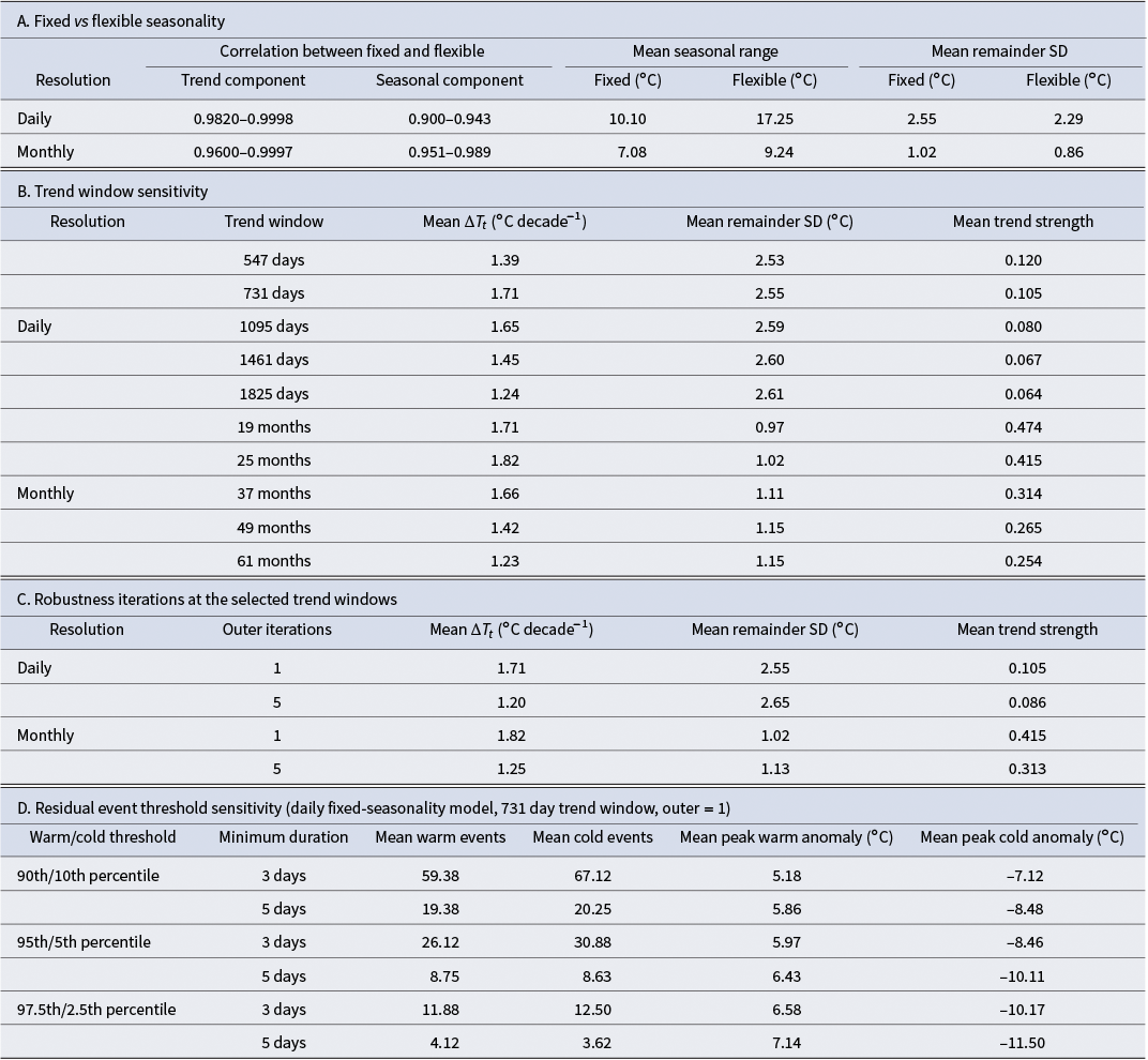
Table II. Long description
Panel A: Fixed versus flexible seasonality. For Daily resolution, the correlation between fixed and flexible is 0.9820 to 0.9998 for the trend and 0.900 to 0.943 for the seasonal component. Mean seasonal range is 10.10 degrees Celsius for fixed and 17.25 degrees Celsius for flexible. For Monthly resolution, trend correlation is 0.9600 to 0.9997 and seasonal is 0.951 to 0.989.
Panel B: Trend window sensitivity. For Daily resolution, as the trend window increases from 547 to 1825 days, the mean trend strength decreases from 0.120 to 0.064. For Monthly resolution, as the window increases from 19 to 61 months, the mean trend strength decreases from 0.474 to 0.254.
Panel C: Robustness iterations. For Daily resolution at 1 outer iteration, mean Delta T sub t is 1.71 degrees Celsius per decade, dropping to 1.20 at 5 iterations. For Monthly resolution, it drops from 1.82 to 1.25 degrees Celsius per decade when moving from 1 to 5 iterations.
Panel D: Residual event threshold sensitivity for the daily model. At the 90th/10th percentile with a 3-day minimum duration, there are 59.38 mean warm events and 67.12 mean cold events. At the 97.5th/2.5th percentile with a 5-day duration, events drop to 4.12 warm and 3.62 cold, with mean peak anomalies of 7.14 and minus 11.50 degrees Celsius respectively.
SD = standard deviation.
By contrast, the St and Rt components are more sensitive to this choice. At the daily scale, the correlation between fixed and flexible St components ranges from 0.900 at SO to 0.943 at CR, and the amplitude of the flexible seasonal component is consistently larger than that of the fixed one. For example, the seasonal range at SO increases from 9.59°C in the fixed model to 23.42°C in the flexible model. At the same time, the standard deviation of the remainder decreases, indicating that the flexible model absorbs part of the variability that, under fixed seasonality, remains assigned to the residual component. A similar, although weaker, pattern is observed at the monthly scale.
These results show that the trend component is robust to seasonal specification, whereas the partitioning between seasonal and residual variability depends more strongly on whether the annual cycle is allowed to vary through time. Full station-by-station comparisons between fixed and flexible seasonality are provided in Table S1.
Sensitivity to the trend window
The decomposition also responds systematically to changes in the trend window (Table II, Fig. S1 & Table S2). In the daily fixed-seasonality models with outer = 1, the mean ΔTt across all stations is 1.39°C 10 yr−1 for a window of 547 days, 1.72°C decade−1 for 731 days, 1.65°C 10 yr−1 for 1095 days, 1.45°C 10 yr−1 for 1461 days and 1.24°C 10 yr−1 for 1825 days. Over the same range, the mean standard deviation of the Rt component increases slightly from 2.53°C to 2.61°C, whereas the mean strength of the trend decreases from 0.120 to 0.064. The monthly fixed-seasonality models show the same general behaviour, with broader trend windows producing weaker trend strength and larger residual variability. Detailed station-by-station responses to alternative trend windows and robustness settings are provided in Table S2. This pattern indicates that shorter windows allow more low-frequency variability to be incorporated into the trend component, whereas broader windows transfer a larger fraction of that variability to the remainder.
Taken together, these results suggest that very short trend windows tend to overrepresent intermediate-term variability in the trend component, whereas very broad windows over-smooth the low-frequency signal and shift too much structure into the remainder.
Sensitivity of residual event thresholds
The residual event analysis follows the expected pattern under alternative threshold definitions. More permissive thresholds, such as the 90th/10th percentiles with a minimum duration of 3 days, produce larger numbers of detected events, whereas stricter definitions, such as the 97.5th/2.5th percentiles and/or a minimum duration of 5 days, produce fewer but more intense events (Table II, Fig. S1 & Table S3). Full station-by-station results of the event threshold sensitivity analysis are provided in Table S3. Despite these differences in absolute event counts, the relative station pattern remains stable. Stations such as JC, CR and SO consistently show comparatively large numbers of residual events, whereas LL and NI tend to show fewer. This indicates that the identification of the most event-prone stations is not strongly dependent on the exact threshold combination adopted.
Selection of the principal model configuration
The sensitivity analysis supports the use of a main model based on fixed seasonality, a daily trend window of 731 days, a monthly trend window of 25 months and one outer robustness iteration (Table II & Fig. S1). Fixed seasonality was retained because it provides a clearer separation between the expected annual cycle and the residual component, which is essential when the remainder is interpreted as an anomaly relative to the mean seasonal structure. The selected trend windows represent an intermediate solution between overfitting short-term variability and over-smoothing interannual evolution. Similarly, the event definition based on the station-specific 95th and 5th percentiles and a minimum duration of 3 days was retained as a balanced compromise between sensitivity to anomalous episodes and avoidance of excessive event fragmentation.
Overall, the sensitivity analysis indicates that the main decomposition model is sufficiently robust for the purposes of this study. In particular, the low-frequency trend remains stable across reasonable alternative parameterizations, whereas the seasonal-residual partition and the number of detected events are more sensitive to model choice, although they preserve the same broad station patterns.
Results
Decomposition structure
Across all stations (Fig. 3), the decomposition shows that near-surface air temperature is primarily structured by a strong annual cycle, whereas the long-term trend accounts for a smaller but persistent fraction of the total variability. This general behaviour is evident in both the daily and monthly decompositions, but it is more clearly expressed at the monthly scale, where short-term noise is reduced and the annual thermal cycle becomes more regular.
Additive decomposition of the selected near-surface air temperature series for the eight study stations at daily (left column) and monthly (right column) resolution (see text for station name abbreviation expansions). For each station, the observed series (Raw), seasonal component, trend component and remainder are shown. Grey vertical bands indicate periods with missing or invalid data in the original records.

Figure 3. Long description
A multi-panel line graph organized into two columns and eight rows. The left column displays Daily resolution data, and the right column displays Monthly resolution data. Each row corresponds to a specific station identified by initialisms: J C, N I, I N, C R, M O, S O, L L, and C L.
Within each of the 16 panels, four distinct time-series components are stacked vertically:
* Raw: A black line showing the observed temperature fluctuations.
* Seasonal: A blue oscillating wave showing regular periodic cycles.
* Trend: A red line showing long-term gradual changes, generally exhibiting a slight upward slope across most stations.
* Remainder: A dark grey line showing residual noise after removing seasonal and trend components.
The X-axis represents time from the year 2000 to 2024. Vertical grey bands of varying widths are interspersed across the timelines, indicating periods of missing or invalid data. These gaps are most prominent in the M O and S O stations around 2014 to 2018. The seasonal blue waves are highly consistent in amplitude and frequency across all panels, while the red trend lines show localized variations, such as a distinct dip in the M O station around 2014.
In the daily fixed-seasonality model (Table III), the strength of seasonality (FS ) ranges from 0.461 at SO to 0.525 at LL, while the strength of trend (FT ) ranges from 0.070 at IN to 0.146 at CL. The remainder component retains a large part of the daily variability, with standard deviations between 2.35°C at LL and 2.87°C at SO. The seasonal amplitude range is relatively similar among stations, varying from 9.59°C at SO to 11.29°C at MO. In the monthly fixed-seasonality model, the annual cycle becomes much more prominent. Here, FS ranges from 0.806 at SO to 0.883 at IN, whereas FT ranges from 0.358 at NI to 0.496 at CL. The standard deviation of the remainder is much lower than in the daily series, ranging from 0.85°C at IN to 1.25°C at SO. The seasonal amplitude range varies between 6.69°C at NI and 7.42°C at MO.
Summary metrics of the selected daily and monthly additive decompositions for each station (see text for station name abbreviation expansions). FS and FT denote the strength of seasonality and of the trend component, respectively; seasonal range is the amplitude range of the seasonal component; remainder SD is the standard deviation of the remainder component; and ΔTt is the decadal-scaled endpoint difference of the smoothed trend component. ΔTt is not a linear trend estimate or a regional atmospheric warming rate.
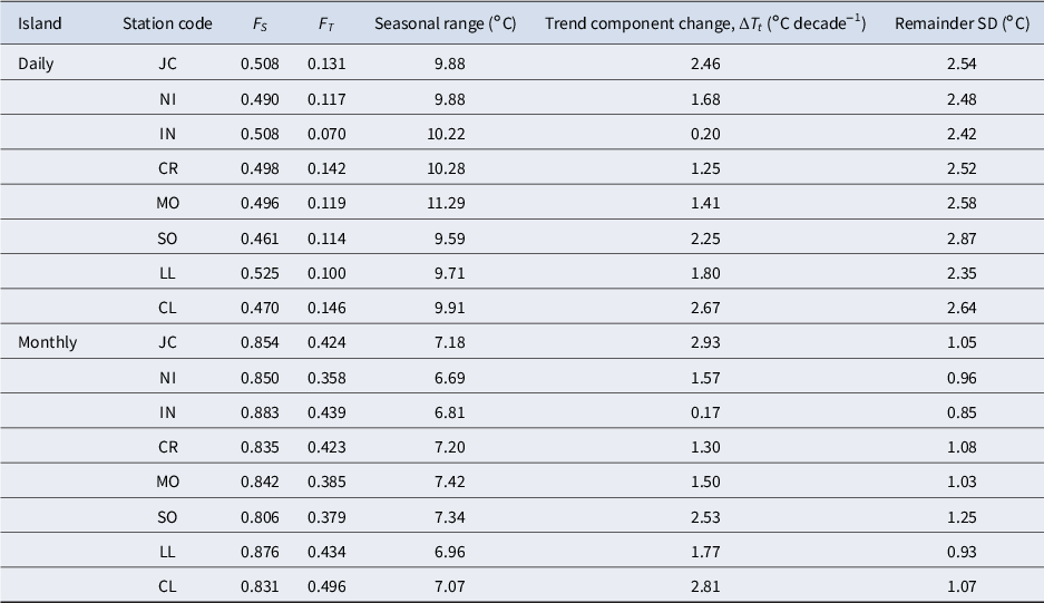
Table III. Long description
The table is divided into two main categories: Daily and Monthly. It contains seven columns: Island (time scale), Station code, F sub S (seasonality strength), F sub T (trend strength), Seasonal range in degrees Celsius, Trend component change (Delta T sub t) in degrees Celsius per decade, and Remainder S D in degrees Celsius.
Daily Section:
* J C: F sub S 0.508, F sub T 0.131, Range 9.88, Trend 2.46, S D 2.54.
* N I: F sub S 0.490, F sub T 0.117, Range 9.88, Trend 1.68, S D 2.48.
* I N: F sub S 0.508, F sub T 0.070, Range 10.22, Trend 0.20, S D 2.42.
* C R: F sub S 0.498, F sub T 0.142, Range 10.28, Trend 1.25, S D 2.52.
* M O: F sub S 0.496, F sub T 0.119, Range 11.29, Trend 1.41, S D 2.58.
* S O: F sub S 0.461, F sub T 0.114, Range 9.59, Trend 2.25, S D 2.87.
* L L: F sub S 0.525, F sub T 0.100, Range 9.71, Trend 1.80, S D 2.35.
* C L: F sub S 0.470, F sub T 0.146, Range 9.91, Trend 2.67, S D 2.64.
Monthly Section:
* J C: F sub S 0.854, F sub T 0.424, Range 7.18, Trend 2.93, S D 1.05.
* N I: F sub S 0.850, F sub T 0.358, Range 6.69, Trend 1.57, S D 0.96.
* I N: F sub S 0.883, F sub T 0.439, Range 6.81, Trend 0.17, S D 0.85.
* C R: F sub S 0.835, F sub T 0.423, Range 7.20, Trend 1.30, S D 1.08.
* M O: F sub S 0.842, F sub T 0.385, Range 7.42, Trend 1.50, S D 1.03.
* S O: F sub S 0.806, F sub T 0.379, Range 7.34, Trend 2.53, S D 1.25.
* L L: F sub S 0.876, F sub T 0.434, Range 6.96, Trend 1.77, S D 0.93.
* C L: F sub S 0.831, F sub T 0.496, Range 7.07, Trend 2.81, S D 1.07.
Spatial contrasts among stations
Although all stations share the same general signal architecture (Fig. 3), the decomposition reveals substantial spatial differences in the relative importance of its components (Fig. 4). On a daily scale, the highest seasonal strength is found at LL (FS = 0.525), whereas the strongest trend component is observed at CL (FT = 0.146) and the weakest at IN (FT = 0.070). At the monthly scale, the same pattern is broadly maintained: IN and LL show the strongest relative seasonality (FS = 0.883 and 0.876, respectively), while CL displays the strongest trend component (FT = 0.496).
Spatial distribution of metrics derived from the selected daily fixed-seasonality decomposition model at the PERMATHERMAL stations on Livingston and Deception islands (see text for station name abbreviation expansions). FS and FT denote the strength of seasonality and the strength of the trend component, respectively; RSD is the standard deviation of the remainder component; and ΔTt is the decadal-scaled endpoint difference of the smoothed trend component. Values are shown within the symbols, and colours indicate their magnitude according to the scales provided.

Figure 4. Long description
The top panel is a regional map of the South Shetland Archipelago including Livingston Island and Deception Island. A 25 km scale bar is in the top-left. A legend in the top-right shows a color gradient from blue (0) to red (3) for four metrics: F S, F T, R S D in degrees Celsius, and Delta T t in degrees Celsius per decade.
Two regional stations are highlighted:
* L L (Northwest): F S 0.525 (green), F T 0.100 (blue), R S D 2.35 (orange), Delta T t 1.80 (light green).
* C L (Southwest): F S 0.470 (green), F T 0.146 (blue), R S D 2.64 (orange), Delta T t 2.67 (orange).
The bottom panel is a high-resolution topographic map of a specific site with a 150 m scale bar. Six stations are detailed via callouts:
* J C (North): F S 0.508, F T 0.131, R S D 2.54, Delta T t 2.46.
* N I (Northeast): F S 0.490, F T 0.117, R S D 2.48, Delta T t 1.68.
* I N (Center): F S 0.508, F T 0.070, R S D 2.42, Delta T t 0.20.
* C R (Southwest): F S 0.498, F T 0.142, R S D 2.52, Delta T t 1.25.
* S O (South): F S 0.461, F T 0.114, R S D 2.87, Delta T t 2.25.
* M O (Southeast): F S 0.496, F T 0.119, R S D 2.58, Delta T t 1.41.
The endpoint difference of the trend component (ΔTt ) also varies markedly between stations (Figs 4 & 5 & Table III). In the daily model, ΔTt reaches 2.67°C 10 yr−1 at CL, 2.46°C 10 yr−1 at JC and 2.25°C 10 yr−1 at SO, whereas lower values are found at CR (1.25°C 10 yr−1), MO (1.41°C 10 yr−1), NI (1.68°C 10 yr−1), LL (1.80°C 10 yr−1) and especially IN, where ΔTt is only 0.20°C 10 yr−1 (Table III). The monthly decomposition yields a very similar station ranking, with the highest ΔTt values again at CL (2.81°C 10 yr−1), JC (2.93°C 10 yr−1) and SO (2.53°C 10 yr−1) and the weakest at IN (0.17°C decade−1). These differences are not limited to the endpoint ΔTt values, but also affect the temporal shape of the low-frequency evolution (Fig. 5). In several stations, especially CL, JC and SO, the trend component (Tt ) shows a clearer upward tendency after the mid-2010s, whereas other stations retain flatter or more irregular trajectories, with Tt exceeding 0°C at some stations (JC, NI and IN).
Comparison of the trend component (Tt ) derived from the selected daily fixed-seasonality decomposition model for the eight study stations (see text for station name abbreviation expansions). Curves show the temporal evolution of Tt , expressed in °C, and allow comparison of the shape and endpoint difference (ΔTt ) of the trend component among stations.

Figure 5. Long description
The x-axis represents years from 2000 to 2024 in two-year increments. The y-axis represents the Trend component in degrees Celsius ranging from negative 7 to 0. Eight colored lines represent different stations: S O (yellow), M O (light green), C R (pink), I N (purple), N I (orange), J C (teal), L L (brown), and C L (blue).
* The S O line starts lowest at negative 7 in 2000, showing high volatility with major troughs near 2008 and 2013 before rising to negative 2 by 2024.
* J C and M O begin around negative 5 and negative 4 respectively in 2000, showing a general upward trend with periodic oscillations.
* Most stations (C R, I N, N I, L L, C L) enter the data set between 2006 and 2010.
* A notable convergence occurs between 2020 and 2024, where almost all lines trend upward toward the 0 degree Celsius mark.
* C L (blue) shows a sharp peak above 0 degrees Celsius around 2021 before stabilizing.
* By 2024, the Delta T sub t endpoint difference shows most stations clustered between negative 1 and positive 0.5 degrees Celsius.
Residual variability and thermal events
The Rt component represents a major part of the signal at the daily scale (Fig. 3 & Table III). In the daily model, the standard deviation of the remainder exceeds 2°C in all stations and reaches its highest value at SO (2.87°C), followed by CL (2.64°C) and MO (2.58°C). Lower but still substantial values occur at LL (2.35°C), IN (2.42°C), NI (2.48°C), CR (2.52°C) and JC (2.54°C). This residual variability also shows clear interannual differences. Years with the largest positive annual sums of the remainder vary by station, including 2010 at CL, 2008 at CR, 2011 at IN, 2006 at JC, 2010 at LL, 2018 at MO, 2007 at NI and 2004 at SO. The largest negative residual sums occur in 2011 at CL, 2007 at CR, 2011 at IN, 2007 at JC, 2011 at LL, 2003 at MO, 2011 at NI and 2005 at SO. Similarly, the annual standard deviation of the remainder reaches particularly high values in 2020 at CL, 2007 at CR and JC, 2011 at IN, LL, and MO, 2007 at NI and 2004 at SO.
Using the selected residual event definition (station-specific 95th/5th percentiles, minimum duration of 3 days), the number of warm events ranges from 21 at NI to 33 at JC, while the number of cold events ranges from 26 at CL to 42 at JC (Fig. 6). In all stations except SO, cold events are slightly more numerous than warm ones. Mean event duration is remarkably consistent across the network, with warm events lasting ~3.9–4.5 days and cold events lasting ~3.7–4.2 days. Mean peak residual magnitude ranges from +5.28°C at LL to +6.97°C at SO for warm events, and from −7.78°C at LL to −9.31°C at SO for cold events.
Annual number of warm and cold residual events detected for each station in the selected daily fixed-seasonality model during 2000–2022 (see text for station name abbreviation expansions). Events were identified from the daily remainder series using station-specific 95th/5th percentile thresholds and a minimum duration of 3 consecutive days. Colour intensity indicates the annual number of events; grey indicates years without detected events; and white indicates periods without data. b. Daily remainder series for the eight stations during May and July 2011. Yellow- and blue-shaded bands indicate detected warm and cold residual events, respectively.

Figure 6.a. Long description
Panel a consists of two heatmaps. The top heatmap, labeled Warm, shows years 2000 to 2022 on the x-axis and eight stations (J C, N I, I N, C R, M O, S O, L L, C L) on the y-axis. Color intensity from yellow to dark red indicates 1 to 7 events. Notable peaks include dark red cells for C R in 2018 and S O in 2004. The bottom heatmap, labeled Cold, uses a blue color scale for 1 to 6 events. A dark purple cell indicates a peak for C R in 2015. Grey cells indicate zero events, and white cells indicate missing data. A legend below panel a maps colors to the number of events.
Panel b contains two line graphs showing Remainder in degrees Celsius on the y-axis against Day of month from 1 to 31 on the x-axis.
* The top graph for May 2011 shows multiple overlapping colored lines for the eight stations. Two yellow-shaded vertical bands indicate warm residual events occurring roughly between days 14 to 17 and 23 to 31, where temperatures peak above 5 degrees Celsius.
* The bottom graph for July 2011 shows two blue-shaded vertical bands indicating cold residual events between days 21 to 25 and 28 to 31, where temperatures drop toward negative 10 degrees Celsius.
A shared legend at the bottom identifies the eight stations by color: J C (dark blue), N I (orange), I N (green), C R (red), M O (cyan), S O (purple), L L (pink), and C L (brown).
Discussion
Seasonal structure
Qualitative assessment of the decomposed series shows a recurrent annual pattern in the seasonal component at all stations, together with a more irregular remainder component, particularly at a daily resolution (Fig. 3). The quantitative metrics confirm that seasonality is the principal organizing component of the series: FS ranges from 0.461 to 0.525 in the daily decomposition and from 0.806 to 0.883 in the monthly decomposition, whereas the standard deviation of the remainder decreases from 2.35–2.87°C at a daily resolution to 0.85–1.25°C at a monthly resolution (Table III). Thus, the monthly decomposition more clearly isolates the stable annual thermal rhythm, while the daily decomposition retains a substantially larger amount of short-term residual variability. This result is consistent with the broader climatology of the Antarctic Peninsula region and, more specifically, with long-term meteorological observations from Livingston and Deception islands, where near-surface air temperature shows a strongly seasonal annual cycle despite marked interannual and decadal variability (Bañón et al. Reference Bañón, Justel, Velázquez and Quesada2013, González et al. Reference González, Vasallo, Recio-Blitz, Guijarro and Riesco2018, González-Herrero et al. Reference González-Herrero, González-Espejo, Jiménez-Cavero, Albero-Molina, Bañon and Aguilar-Pérez2026). In that sense, the decomposition does more than confirm the obvious presence of seasonality: it quantifies the extent to which the annual cycle provides the temporal framework within which both background evolution and anomalous short-term departures operate (Turner et al. Reference Turner, Colwell, Marshall, Lachlan-Cope, Carleton and Jones2005, Reference Turner, Marshall, Clem, Colwell, Phillips and Lu2020, Carrasco et al. Reference Carrasco, Bozkurt and Cordero2021).
This interpretation is also in line with the few Antarctic applications of STL-type decompositions published so far. Carter et al. (Reference Carter, Leeson, Orr, Kittel and van Wessem2022) showed that monthly Antarctic climate fields can be meaningfully partitioned into seasonal, trend and residual components, while Kwok et al. (Reference Kwok, Qian and Kuleshov2023) showed that LOESS-based decomposition can recover stable long-term behaviour even from temperature series with missing data, provided that the underlying signal is sufficiently smooth. Although those studies do not analyse a station-based Maritime Antarctic network comparable to the present one, they support the broader methodological conclusion that decomposition is particularly informative when the signal contains a strong annual cycle superimposed on lower-frequency change and irregular short-term variability (Carter et al. Reference Carter, Leeson, Orr, Kittel and van Wessem2022, Kwok et al. Reference Kwok, Qian and Kuleshov2023).
At the same time, the results make clear that seasonality does not explain the full behaviour of the air temperature series. Even after removal of the recurrent annual cycle, substantial structure remains in both the trend and the remainder. This is important because it shows that the recent thermal evolution of the South Shetland Islands cannot be reduced to a simple repetition of the same seasonal pattern with a small long-term correction. Instead, the temperature signal is built from three interacting components: a strong annual rhythm, a lower-frequency background evolution and short-term departures that may be large and persistent. In this sense, decomposition provides a more informative framework than annual means or raw trend estimates alone because it explicitly separates processes acting at different temporal scales (Cleveland et al. Reference Cleveland, Cleveland, McRae and Terpenning1990, Carter et al. Reference Carter, Leeson, Orr, Kittel and van Wessem2022, Kwok et al. Reference Kwok, Qian and Kuleshov2023).
Spatial contrasts between stations
The station comparison shows that the network cannot be interpreted as a simple lapse-rate transect, even though elevation clearly provides the first-order framework. On Hurd Peninsula, the lower stations define the warm end of the Livingston transect, whereas the upper sites, especially SO, represent progressively colder conditions with increasing altitude (Table I). However, the inclusion of LL on Byers Peninsula and CL on Deception Island shows that the spatial structure of the network is more complex than a simple elevation gradient. LL and CL lie at similar elevations, yet they do not behave identically, which suggests that mean air temperature is shaped not only by altitude but also by local exposure, topographic shelter, degree of maritime influence and island-specific environmental conditions. This interpretation is consistent with the broader climatic literature for the South Shetland Islands (González-Herrero et al. Reference González-Herrero, González-Espejo, Jiménez-Cavero, Albero-Molina, Bañon and Aguilar-Pérez2026), which shows that surface temperature variability is influenced by both large-scale atmospheric forcing and local controls (Torres et al. Reference Torres, Bozkurt and Arigony-Neto2023).
The magnitude of these ΔTt values (Fig. 5) must nevertheless be interpreted in the context of the relatively short and partly non-coincident observation periods, since temperature changes estimated over short Antarctic Peninsula records may be strongly affected by the selected initial and final years and can be considerably larger than changes derived from longer records (Gonzalez & Fortuny Reference Gonzalez and Fortuny2018). The endpoint differences in Tt are spatially heterogeneous, even across this relatively compact regional network (Fig. 4). If elevation alone controlled the low-frequency evolution of the series, one would expect a smoother progression of ΔTt from the lower Hurd Peninsula stations to SO. Instead, the highest ΔTt values occur at CL, JC and SO, while IN shows a much weaker low-frequency change. Importantly, these ΔTt values describe endpoint differences in the smoothed component over the available observation periods and should not be interpreted as linear warming rates directly comparable with long-term meteorological trends. As shown by Gonzalez & Fortuny (Reference Gonzalez and Fortuny2018), temperature trends calculated over relatively short intervals in the Antarctic Peninsula may be strongly influenced by the selected start and end years, especially when the interval spans contrasting phases of regional temperature evolution. This pattern is entirely plausible in the Antarctic Peninsula region, where warming has long been recognized as spatially heterogeneous, seasonally uneven and strongly modulated by atmospheric circulation rather than being expressed as a uniform regional trend (Turner et al. Reference Turner, Colwell, Marshall, Lachlan-Cope, Carleton and Jones2005, Reference Turner, Marshall, Clem, Colwell, Phillips and Lu2020, Oliva et al. Reference Oliva, Navarro, Hrbáček, Hernández, Nývlt and Pereira2017, Carrasco et al. Reference Carrasco, Bozkurt and Cordero2021). The particularly low ΔTt value at IN is therefore identified here as a station-scale contrast, but its physical origin cannot be established from the decomposition alone. Possible influences such as local exposure, topographic setting, snow conditions or site-specific observational effects would require targeted analyses using additional meteorological, snow cover and instrumental comparison data.
A useful way to read the network, therefore, is to distinguish between mean thermal structure and recent background evolution (Figs 3 & 4). The first is broadly organized by altitude and by island-scale setting. The second is more locally modulated. CL and SO are especially informative in this regard: CL combines a relatively mild mean state with one of the strongest decomposed trend signals, whereas SO combines the coldest mean conditions with one of the strongest low-frequency changes. These two cases suggest that local controls influence not only the baseline thermal regime of each site, but also the way in which regional atmospheric change is expressed at the station scale. This interpretation is also consistent with published ground thermal studies from the same islands. Interannual analyses of ground surface thermal regimes in Livingston and Deception islands show marked site-to-site differences and a strong influence of local conditions, especially snow cover, on thermal behaviour, while work from the Mount Reina Sofía sector (SO site) has shown that increased snow accumulation can even drive a transition from a subaerial to a sub-nival permafrost temperature regime (Ramos et al. Reference Ramos, Vieira, de Pablo, Molina and Jiménez2020, de Pablo et al. Reference de Pablo, Ramos, Vieira, Molina, Ramos and Maior2024, Reference de Pablo, Bermejo, Goyanes and Sánchez2026). Together, these results indicate that local controls modulate not only baseline climate but also the way in which regional atmospheric change is expressed at the station scale.
Residual variability
One of the clearest contributions of this study is that the remainder contains substantial and spatially structured variability that merits interpretation, while recognizing that it may also include observational noise, unresolved seasonal structure and decomposition-related effects (Figs 3 & 4 & Table III). At the daily scale, residual variability remains substantial in all stations after the annual cycle and low-frequency component have been removed. More importantly, it is not distributed uniformly across the network. SO has the strongest residual variability, followed by CL and MO, whereas LL shows the weakest residual variability. This means that some stations are not only warmer or colder than others, but also more thermally irregular once their expected seasonal behaviour is removed. In that sense, the remainder provides an operational measure of each site’s tendency to depart from its estimated seasonal and low-frequency behaviour. The spatial contrasts identified here are consistent with differences in local thermal response, but their attribution to specific meteorological or environmental controls requires additional evidence. This contrast (Fig. 4 & Table III) is particularly informative when comparing LL and CL. Despite their similar elevation, they differ markedly in their residual behaviour. Similarly, SO combines the coldest mean state with the strongest residual variability, showing that the coldest site is not the most stable one. Recent direct snow-depth monitoring within the PERMATHERMAL network provides observational support for considering local snow conditions among the factors potentially contributing to these contrasts. During the 2023–2024 snow season, de Pablo & Rosado (Reference de Pablo and Rosado2026) documented strongly heterogeneous snow accumulation across the same monitoring areas: LL showed a progressive increase in snow depth exceeding 1 m, whereas closely spaced sites in the CL sector recorded markedly contrasting snow depths, from less than 20 cm to more than 80 cm. At SO, the snow-depth record could not be evaluated for the complete season because the ultrasonic sensor support failed in mid-August 2023.
This spatial heterogeneity is relevant because previous work in the Mount Reina Sofía sector, where SO is located, showed that increased snow accumulation can shift the ground thermal regime from subaerial to sub-nival conditions (Ramos et al. Reference Ramos, Vieira, de Pablo, Molina and Jiménez2020). However, the snow-depth observations reported by de Pablo & Rosado (Reference de Pablo and Rosado2026) postdate the air temperature series analysed here, and the ground thermal response described by Ramos et al. (Reference Ramos, Vieira, de Pablo, Molina and Jiménez2020) cannot be directly extrapolated to the residual component of near-surface air temperature. Consequently, these studies do not demonstrate that snow conditions caused the residual behaviour identified for individual stations, but they provide a physically supported basis for considering snow cover, together with exposure, topographic shelter and island setting, as plausible controls requiring future concurrent snow-depth and meteorological analyses.
The seasonal structure of the remainder (Fig. 3) supports that interpretation. In the present dataset, residual variability is systematically smallest in summer and largest in winter, with autumn and spring occupying intermediate positions. This is physically coherent. During summer, temperatures are more tightly constrained by the annual thermal cycle, whereas in winter the atmosphere is more strongly affected by advection, wind variability and circulation changes, which can generate large departures from the expected seasonal baseline (van den Broeke & van Lipzig Reference van den Broeke and van Lipzig2004, González et al. Reference González, Vasallo, Recio-Blitz, Guijarro and Riesco2018, Bozkurt et al. Reference Bozkurt, Marín and Barrett2022). This interpretation also agrees with recent analyses of ground surface temperature from Livingston and Deception islands, which show that the thermal year is organized into distinct phases and that the onset of winter is strongly conditioned by snow cover development and the transition from atmospheric control to snow-insulated conditions (de Pablo et al. Reference de Pablo2025). The remainder therefore appears to capture the season in which atmospheric irregularity is greatest and most likely to produce contrasting local responses before snow cover attenuates or reorganizes the surface thermal signal.
Warm and cold residual events
The residual event catalogue (Fig. 6) adds a useful comparative layer because it allows periods of marked residual departure to be compared across stations and across years. Several clear patterns emerge:
-
• Cold residual events are slightly more numerous than warm ones in most stations. This is true at CL, CR, IN, JC, LL, MO and NI, whereas SO is closer to a balance between the two types. This pattern adds a useful comparative dimension, highlighting periods when observed temperatures depart markedly from the estimated seasonal and trend components. Overall, negative residual departures remain common within the analysed series.
-
• Event frequency is not distributed evenly across the network: JC tends to record the highest number of both warm and cold events, whereas LL and NI generally record fewer warm and cold events.
-
• The largest peak magnitudes are recorded at SO for both warm and cold events, indicating that the highest and coldest station is also one of the most responsive to anomalous departures. This suggests that mean thermal state and anomaly magnitude do not vary in parallel.
The annual distribution of events (Fig. 6) also provides useful comparative information. In the present dataset, 2011 stands out for widespread warm residual event activity, whereas 2015 shows widespread cold residual event activity. These patterns are derived from the remainder component and therefore do not identify their meteorological causes; however, they can be considered in the context of the marked interannual variability and the cooling or hiatus conditions reported for parts of the Antarctic Peninsula during the early twenty-first century (Oliva et al. Reference Oliva, Navarro, Hrbáček, Hernández, Nývlt and Pereira2017, Carrasco et al. Reference Carrasco, Bozkurt and Cordero2021). Their occurrence across several stations indicates temporal coherence in residual behaviour within the network, while differences in magnitude show that the response was not identical at all sites. A shared regional influence is therefore plausible, but its atmospheric origin and any local modulation by station setting cannot be established from the decomposition alone. This becomes even clearer when simultaneous events are considered. In the fixed-seasonality daily model, a warm event in late May 2011 is detected in all eight stations, and the same occurs for a cold event in late July 2011 (Fig. 6). The temporal coincidence of these residual events across the eight stations is consistent with a shared regional influence, although the decomposition does not establish whether they resulted from the same atmospheric disturbance, nor does it identify its mechanism. Regional atmospheric forcing and its possible local modulation by relief, elevation and exposure provide a plausible interpretive framework for such spatially coherent residual behaviour based on previous studies of Antarctic Peninsula temperature variability and extremes (Turner et al. Reference Turner, Marshall, Clem, Colwell, Phillips and Lu2020, Reference Turner, Lu, King, Marshall, Phillips, Bannister and Colwell2021).
This interpretation is also consistent with recent work on Antarctic Peninsula warm events. Atmospheric rivers, strong warm air advection and föhn effects are now recognized as major contributors to warm anomalies and melt episodes in the region, especially where local topography enhances the surface response (Cape et al. Reference Cape, Vernet, Skvarca, Marinsek, Scambos and Domack2015, van Wessem et al. Reference van Wessem, Reijmer, van de Berg, van den Broeke, Cook, Van Ulft and van Meijgaard2015, Bozkurt et al. Reference Bozkurt, Marín and Barrett2022, Gorodetskaya et al. Reference Gorodetskaya, Durán-Alarcón, González-Herrero, Clem, Zou and Rowe2023, Zou et al. Reference Zou, Rowe, Gorodetskaya, Bromwich, Lazzara and Cordero2023). The February 2022 Antarctic Peninsula event is perhaps the clearest recent example, combining an intense atmospheric river with föhn amplification and producing exceptional surface warming and melt (Gorodetskaya et al. Reference Gorodetskaya, Durán-Alarcón, González-Herrero, Clem, Zou and Rowe2023, Zou et al. Reference Zou, Rowe, Gorodetskaya, Bromwich, Lazzara and Cordero2023). More broadly, intense atmospheric rivers have been identified as important contributors to extreme surface melt and ice-shelf destabilization across the Antarctic Peninsula sector, often in combination with down-sloping föhn winds on the lee side of the mountain barrier (Laffin et al. Reference Laffin, Zender, van Wessem and Marinsek2022, Wille et al. Reference Wille, Favier, Jourdain, Kittel, Turton and Agosta2022). The present decomposition does not identify the synoptic cause of each event, but it provides something equally useful: an objective way to flag when anomalous warm or cold periods occurred, which stations recorded them and how strong the local response was at each site. In that sense, the remainder provides an effective bridge between station climatology and synoptic interpretation.
Frozen ground implications
The station comparison (Figs 3 & 5) has direct implications for frozen ground because the same atmospheric forcing is being imposed on sites that are not equally close to critical thermal thresholds. The lower Hurd Peninsula stations are already at the warm end of the network, whereas SO remains the most freezing-dominated station and CR/MO occupy intermediate positions. This means that the same regional warming signal and the same anomaly regime are acting on ground systems with different initial thermal states and, therefore, different sensitivities. The distinction matters because frozen ground in the South Shetland Islands is widely regarded as thermally marginal and spatially heterogeneous, close to its climatic stability limit (Vieira et al. Reference Vieira, Bockheim, Guglielmin, Balks, Abramov and Boelhouwers2010, Bockheim et al. Reference Bockheim, Vieira, Ramos, López-Martínez, Serrano and Guglielmin2013, Obu et al. Reference Obu, Westermann, Vieira, Abramov, Balks and Bartsch2020, Hrbáček et al. Reference Hrbáček, Oliva, Hansen, Balks, O’Neill and de Pablo2023). In these environments, snow duration, thickness and physical properties are key controls on ground thermal behaviour and permafrost occurrence, so relatively modest differences in local snow and site setting may substantially alter the way atmospheric forcing is transferred to the ground (Ferreira et al. Reference Ferreira, Vieira, Ramos and Nieuwendam2017).
CL and SO are especially informative end-members (Fig. 4). CL combines one of the highest ΔTt values with a locally distinctive setting on Deception Island, whereas SO combines the coldest baseline with a high ΔTt value and the largest residual variability. These stations therefore illustrate two potentially different forms of thermal sensitivity. At CL, the high ΔTt value identifies a marked endpoint difference in the trend component during the available observation period, which may be relevant for already marginal frozen ground. SO, by contrast, may retain a colder average state but shows particularly high residual variability, suggesting greater short-term departures from its estimated seasonal and low-frequency behaviour (Figs 3 & 4). This distinction shows that frozen ground sensitivity in Maritime Antarctica cannot be inferred from mean air temperature alone. It depends on the interaction between mean state, low-frequency evolution, short-term residual departures, snow conditions and local environmental controls. This interpretation is strongly supported by the ground thermal literature from the same network. Interannual analyses of ground surface thermal regimes in Livingston and Deception islands show marked spatial contrasts and year-to-year variability in ground thermal behaviour, whereas work from the Mount Reina Sofía sector (SO station) and Crater Lake region (CL station) has demonstrated that increased snow accumulation can even shift permafrost from a subaerial to a sub-nival thermal regime (Ramos et al. Reference Ramos, Vieira, de Pablo, Molina, Abramov and Goyanes2017, Reference Ramos, Vieira, de Pablo, Molina and Jiménez2020, de Pablo et al. Reference de Pablo, Ramos, Vieira, Molina, Ramos and Maior2024).
That broader interpretation is also consistent with recent analyses of surface thermal phases from the same islands. Ground surface temperature records from Livingston and Deception islands indicate that soils undergo a comparable early-winter cooling phase before a shallow snow mantle covers the sites, after which snow insulation becomes a major control on thermal behaviour (de Pablo et al. Reference de Pablo2025). This means that the atmospheric variability identified here through decomposition is unlikely to be transferred uniformly to the ground throughout the year. Rather, its effects will depend on when anomalous atmospheric forcing occurs relative to snow onset, snow persistence and site-specific surface conditions. At the broader scale, permafrost in the Antarctic Peninsula region is comparatively warm and close to thaw thresholds in many coastal and island settings, and pan-Antarctic syntheses and modelling show that near-surface permafrost temperatures in the Maritime Antarctic are much less negative than in most of Continental Antarctica (Bockheim et al. Reference Bockheim, Vieira, Ramos, López-Martínez, Serrano and Guglielmin2013, Obu et al. Reference Obu, Westermann, Vieira, Abramov, Balks and Bartsch2020, Hrbáček et al. Reference Hrbáček, Oliva, Hansen, Balks, O’Neill and de Pablo2023). Antarctica has also already shown measurable permafrost warming as part of the global pattern of permafrost temperature increase (Biskaborn et al. Reference Biskaborn, Smith, Noetzli, Matthes, Vieira and Streletskiy2019). In that context, the present results add a useful refinement: atmospheric forcing in the South Shetland Islands should not be viewed only as a gradual increase in mean air temperature but as the combined effect of a strong annual cycle, a spatially heterogeneous background evolution and a substantial short-term anomaly regime, all of which may be filtered and reorganized by local snow and ground conditions before being expressed in the frozen ground.
Methodological considerations
From a methodological perspective, the value of the decomposition lies in its ability to separate three aspects of the temperature signal that are often discussed together but not explicitly partitioned: the recurring annual cycle, the low-frequency background evolution and short-term anomalies. More broadly, classical time-series analysis has long treated the separation of trend, seasonality and irregular variability as a fundamental step in understanding structured temporal data, particularly when the aim is to distinguish recurrent behaviour from long-term change and short-term departures (Brockwell & Davis Reference Brockwell and Davis2016, Hyndman & Athanasopoulos Reference Hyndman and Athanasopoulos2021). Previous Antarctic applications have already included STL decomposition of gridded near-surface air temperature fields, observational upper-air temperature series and soil temperature records, as well as LOESS-based analyses of near-surface air temperature at several stations used in the present study (Carter et al. Reference Carter, Leeson, Orr, Kittel and van Wessem2022, Recondo et al. Reference Recondo, Corbea-Pérez, Peón, Pendás, Ramos and Calleja2022, Kwok et al. Reference Kwok, Qian and Kuleshov2023, Schaefer et al. Reference Schaefer, Francelino, Pereira, Michel, Schmitz and Sacramento2023). Within this established methodological context, the present study provides a comparative analysis of the seasonal, low-frequency and remainder components of multi-year near-surface air temperature series across eight stations in a compact Maritime Antarctic monitoring network. At the same time, the limitations should be stated clearly. The trend component (Tt ) is a smoothed background component and is not equivalent to a regression slope or a regional atmospheric warming rate. The remainder identifies departures relative to the estimated seasonal and low-frequency (trend) components, but it does not reveal their physical cause. It may also include observational noise, unresolved seasonal structure and decomposition-related effects, and it should therefore not be interpreted automatically as a set of physically explained climatic anomalies. Its interpretation requires a distinction between residual patterns demonstrated by the decomposition, possible physical controls suggested by external evidence and causal mechanisms that cannot be established without additional meteorological analysis. In addition, the exact partition between seasonality and residual variability depends partly on model settings, especially when flexible seasonality is allowed. The sensitivity analysis is therefore an essential part of the interpretation rather than a secondary technical exercise. In the present case, it shows that the trend component is highly robust, whereas the seasonal-residual partition is more model dependent and should therefore be interpreted with greater caution (Cleveland et al. Reference Cleveland, Cleveland, McRae and Terpenning1990, Carter et al. Reference Carter, Leeson, Orr, Kittel and van Wessem2022, Kwok et al. Reference Kwok, Qian and Kuleshov2023).
A further limitation concerns the external comparability of the PERMATHERMAL records. These series have not yet been systematically cross-validated against the nearby official meteorological observations available on Livingston and Deception islands. Consequently, the present results should be interpreted as relative temporal and spatial patterns within the PERMATHERMAL network rather than as externally validated estimates directly comparable with those derived from standard meteorological stations. A dedicated comparison with the nearby official observations, including the assessment of possible site- and sensor-related differences, represents a necessary step for future atmospheric applications of the network.
Beyond its use for interpreting the present network, this framework also opens two natural lines of future work. First, the explicit partitioning of the signal into seasonal, trend and residual components provides a useful basis for subsequent forecasting experiments, since decomposition is commonly treated as a preliminary step before time-series modelling and prediction (Brockwell & Davis Reference Brockwell and Davis2016, Hyndman & Athanasopoulos Reference Hyndman and Athanasopoulos2021). Second, and more directly relevant to the PERMATHERMAL network, the same approach could be extended to ground surface (de Pablo et al. Reference de Pablo, Ramos, Vieira, Molina, Ramos and Maior2024, Reference de Pablo, Bermejo, Goyanes and Sánchez2026) and shallow ground temperature series in order to examine how atmospheric seasonality, background evolution and short-term anomalies are transferred, damped or delayed within the frozen ground system.
Conclusions
This study shows that near-surface air temperature in Livingston and Deception islands is primarily structured by a strong annual cycle. This seasonal component provides the main temporal framework of the series, especially at the monthly scale, and confirms that recent atmospheric change in the South Shetland Islands is superimposed on a still strongly recurrent polar thermal regime.
The decomposed trend component indicates a positive background evolution at most stations, but its magnitude is spatially heterogeneous. The thermal evolution of the network does not follow a simple altitudinal pattern, which suggests that local factors such as exposure, topographic and geological setting and island context play an important role in modulating the regional atmospheric signal. The comparison among stations also shows that the decomposed thermal signal is not expressed uniformly across the network. Sites such as CL and SO stand out because they combine strong background evolution with high residual variability or locally distinctive environmental settings, whereas others, such as IN, show much weaker low-frequency change. This confirms that station setting strongly modulates the local expression of regional atmospheric variability.
The remainder is also a significant part of the signal. At the daily scale, it contains substantial residual variability and identifies marked short-term residual departures as an important component of the thermal variability of the network. These residual departures are not randomly distributed, showing both seasonal structure and marked differences among stations.
Residual warm and cold events show that some periods of marked residual departure are coherent across stations, while their local intensity varies from one station to another. This spatial coherence is consistent with a shared regional influence, although its atmospheric origin and any local modulation cannot be established from the decomposition alone. These results are especially relevant for frozen ground studies in Maritime Antarctica, where many sites are already close to thermal thresholds. In such environments, both low-frequency atmospheric change and recurrent positive residual departures may influence thaw timing, active-layer development and the climatic stability of marginal permafrost, although their effective transfer to the ground depends on snow cover, surface characteristics and other local controls.
Overall, the study shows that additive decomposition is a useful framework for analysing Maritime Antarctic air temperature series, even when gaps are present, because it makes it possible to separate the annual seasonal structure, the background thermal evolution and the short-term residual variability in a way that is both climatologically interpretable and spatially comparable.
Supplementary material
The supplementary material associated with this article includes one supplementary figure and three supplementary tables. Figure S1 provides a graphical overview of the sensitivity analysis, including the comparison between fixed and flexible seasonality, the response of the decomposition to alternative trend windows and the effect of alternative residual event thresholds. Table S1 presents the station-by-station comparison between fixed and flexible seasonality. Table S2 summarizes the station-by-station sensitivity of the decomposition to alternative trend windows and robustness settings. Table S3 provides the station-by-station results of the residual event threshold sensitivity analysis. Together, these materials document the robustness of the selected model configuration and complement the summary presented in Table II.
Acknowledgements
The authors thank the chiefs and crews of the Spanish Antarctic stations Juan Carlos I (Livingston Island) and Gabriel de Castilla (Deception Island) for their support during fieldwork and for their assistance with instrument maintenance throughout the 2000–2022 period. The authors also thank the personnel of the Spanish Polar Committee and the crews of the Spanish research vessels Las Palmas, Hespérides and Sarmiento de Gamboa for logistical support during Antarctic operations. In addition, the authors thank the Spanish and Portuguese colleagues who contributed to station maintenance and data downloads during the monitoring period. During the preparation of this manuscript, the authors used the ChatGPT 5.5 Thinking model to assist with 1) figures production using R language, 2) translation from Spanish into English and 3) language revision, including grammar and spelling correction. After using this tool, the authors carefully reviewed and edited the text as needed, and they take full responsibility for the content of the publication. We also thank the reviewers and editors for their detailed and constructive comments, which helped improve the clarity, methodological robustness and overall presentation of the manuscript.
Author contributions
Conceptualization: MAdP; methodology: MAdP and GG; validation: GG; formal analysis: MAdP; investigation: MAdP and GG; data curation: MAdP; writing - original draft preparation: MAdP; writing - review and editing: MAdP and GG; project administration: MAdP. funding acquisition: MAdP. Both authors have read and agreed to the published version of the manuscript.
Financial support
This research was supported by the Spanish Polar Research Program through the projects RADIANTAR (ANT98-057 and REN2001-5082-E/ANT), PERMAMODEL (POL2006-01918), PERMAPLANET (CTM2009-10165), ANTARPERMA (CTM2011-15565-E) and PERMASNOW (CTM2014-52021-R), as well as through the PERMATHERMAL contracts established between Uuniversidad de Alcalá (UAH) and Instituto Geológico y Minero de España (2015–2019, under LOU Article 83) and between UAH and Unidad de Tecnología Marina (2020–2025, under LOSU Article 60).
Competing interests
The authors declare no competing interests. The funders had no role in the design of the study; in the collection, analyses or interpretation of data; in the writing of the manuscript; or in the decision to publish the results.

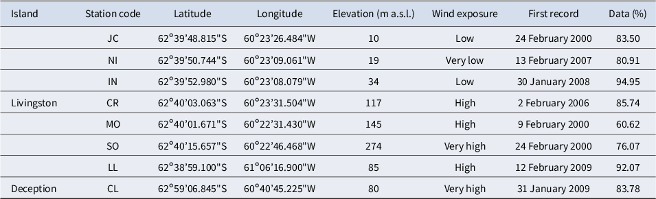
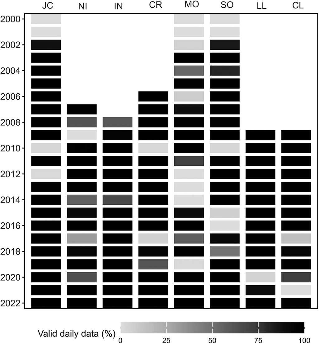
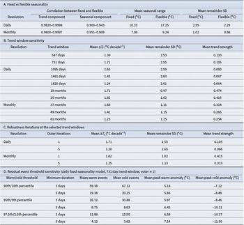

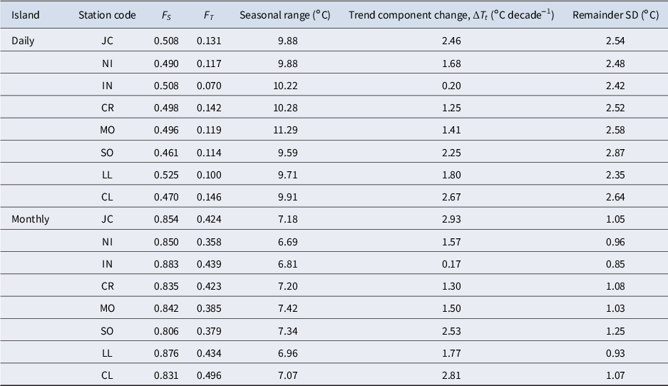


 Open access

