The Development of the Manufacturing Belt

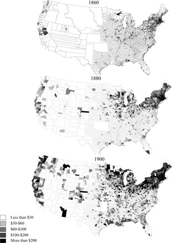
Popularized by Sten DeGreer (Reference DeGeer1927), the concept of the Manufacturing Belt describes a geographic region that became the heart of American industrial activity. Historians illustrate the Belt as a parallelogram with points at Milwaukee, St. Louis, Baltimore, and Boston. As seen in Figure 1, the description is a useful approximation, but ignores the large within-region variation. For example, the agricultural areas of western Indiana and southern Illinois are included in the region, yet the industrial areas south of Baltimore are not included. Pockets of manufacturing developed in western North Carolina and California, yet the Manufacturing Belt still produced over 50 percent of the country's industrial goods through 1970.

Early manufacturing was often determined by the location and size of demand. Due to high transportation costs, manufacturers could not operate far from natural resources or produce significantly more than the local market was willing to consume. Most entrepreneurs, therefore, did not have the incentive to greatly expand production. Despite these constraints, entrepreneurs in key industries developed new production techniques, leading to a buildup of information over time. Meyer (Reference Meyer2006) shows that machinists created a network to share technology, whereas Ross Thomson (Reference Thomson2009) describes how technological progress in one industry carried over to the machines of another. The last decades of the antebellum period, in particular, were a time of innovation that set the stage for the rise of factories (North Reference North1961; Field Reference Field1978). The Manufacturing Belt took shape after the Civil War. First, postbellum firms tended to locate in the Midwest. While manufacturing was expanding in every region of the country, the Northeast states’ shares of U.S. manufacturing output and capital declined from over three-fifths in 1850 to just over half in 1900, whereas the Midwest's shares grew from 12 percent to almost 25 percent over the same period (Haines Reference Haines2004). While these data suffer from inconsistent measurement over time, they still provide evidence of a tremendous shift of production.Footnote ⁴ Second, firms across the Belt invested more heavily in capital goods. The ratio of depreciable capital to net income in current prices remained the same from 1840 to 1860, but grew 11 percent during the 1860s, 20 percent in the 1870s, 8 percent in the 1880s, and 15 percent in the 1890s (Davis and Gallman Reference Davis, Gallman, Mathias and Postan1978, Table 4). Atack, Bateman, and Margo (Reference Atack, Bateman and Margo2003, Reference Atack, Bateman and Margo2008) argue that the capital deepening was due to the adoption of steam engines. The engines allowed establishments to shift away from running water, operate year-round, and increase their total factor productivity.Footnote ⁵ Third, establishments increased their scale of production after Civil War (O'Brien Reference O'Brien1988). Alfred Chandler (Reference Chandler1977) also highlights the growing importance of multi-unit firms and salaried managers.

FIGURE 1

EVOLUTION OF THE MANUFACTURING OUTPUT PER CAPITA (1860–1900)

Notes: Displays county-level value of output per capita. Counties with fewer than 2,000 people or more than 6,500 square miles are given zero values to provide a better comparison. Sources: County boundaries are from Minnesota Population Center (2004). Output per capita are from Haines (2004).

Urbanization and railroad development help explain why the scale of production and capital investment could expand, but they cannot explain why factories were established in some counties but not in others. Because of the scale of investment, I focus my attention on the nation's banking system. Joseph Schumpeter (Reference Schumpeter1912) and Ronald McKinnon (Reference McKinnon1973) posit that banking spurs innovation by attracting deposits and funding entrepreneurs with the best chance of successfully implementing technology. Unlike today, postbellum banks subscribed to the Real Bills Doctrine, issuing short-term self-liquidating loans. Banks provided de facto long-term funds to their regular customers by rolling over debt, but the majority of loans provided operational liquidity, bridged seasonal needs, and helped purchase small capital improvements. They thus were more likely to fund the purchase of steam engines rather than the construction of large factories. Maybe more important for the period, however, the availability of working capital loans would have freed up an establishment's own funds for investment.

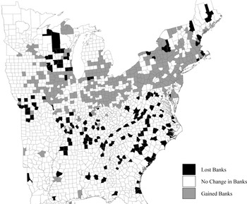
Howard Bodenhorn and David Cuberes (Reference Bodenhorn and Cuberes2010) and Scott Fulford (Reference Fulford2012) show that a bank's presence (or lack thereof) influenced the speed of local economic growth, but no study to date has examined the effect of the National Banking Acts of 1863 and 1864. Between 1863 and 1866 the banking system increased by over 350 banks and $40 million in capital and the geographic distribution of banks shifted towards the Manufacturing Belt. Figure 2 shows that Midwest and Middle Atlantic counties gained banks, New England counties largely kept the same number of banks, and Southern counties lost a large number of banks. The rest of the article looks at these specific changes and whether they contributed to the postbellum's distribution of manufacturing.

FIGURE 2

GERMANY'S TERRITORIAL LOSSES, 1919–1945

Notes: Figure contains the aggregate change in the total number of national and state banks between December 1862 and December 1866. Bank branches are treated as separate banks. Sources: See Data Section for banking sources. County boundaries are from Minnesota Population Center (2004).

Finance and Growth Data

To provide a comprehensive examination of U.S. manufacturing and banking, I assemble a nationwide bank database from 1850 to 1900. The majority of the data come from the Merchants and Bankers’ Directory (1860–1880) and Rand McNally Bankers’ Directory (1890–1900). The bank directories (1881, p. vi) reportedly provide “full lists, carefully constructed, of The National Banks, State Banks, and Private Bankers of every city and town in the United States.” The directories include the name and location of each bank, as well as whether they were chartered by a state legislature (called a state bank), the Comptroller of the Currency (called a national bank), or had no formal charter (called a private banker).Footnote ⁶ I construct the county-level database by counting national and state banks that were in operation and their capital from the directory containing information closest to the end of the specified year.Footnote ⁷ I also separately count the number of private bankers in 1860, but lack of consistent data prevents me from extending the count further in either direction. Due to data availability, I link the database to Weber's antebellum databases (Reference Weber2005, Reference Weber2008) to measure the number of banks and value of bank capital in 1850. The resulting database is the most extensive source of bank information available for the period.

I link the banking census to two separate manufacturing databases. The first is the county-census database assembled by Michael Haines (Reference Haines2004). The database contains the number of manufacturing establishments as well as their aggregate capital and output. In order to construct a consistent panel from 1850 to 1900, I aggregate counties to their 1850 borders and drop out any county group whose data was not reported or had missing values.Footnote ⁸ I also drop out Confederate states so that there is no chance to misconstrue the effect of the National Banking Acts with the destruction in the South during the Civil War. The resulting panel contains decennial observations for 758 county units (representing 864 counties) in 22 states.

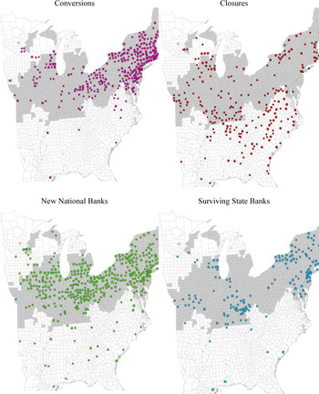
As seen in Figure 3, the sample covers every county in the Northeast and Midwest. The few missing Midwest states were not able to be included because their data were not reported in 1850, where the few missing counties were typically sparsely populated areas that had not yet been formed into a county. The analysis is thus conducted on variation within the Manufacturing Belt itself. The effect of banks within the core region, where the financial system was more developed, should arguably set a lower bound on the effect of banks in the periphery, where the financial system was less developed.

FIGURE 3

LOCATIONS OF CONVERSIONS, CLOSURES, ENTRY, AND SURVIVING BANKS (1860–1866)

Notes: Displays the changes in national and state banks across the period where the size of the dot denotes the number of banks. Bank branches are treated as separate banks. Shaded areas denote counties in the sample. Sources: See Data Section for banking sources. County boundaries are from Minnesota Population Center (2004).

The second is the establishment-level database collected by Atack and Bateman (Reference Atack and Bateman1999). The authors formed the database by drawing representative samples of establishments from the 1850, 1860, 1870, and 1880 Census of Manufacturing. The database contains the base information for the variables in the county-level data, as well as other characteristics that were not tabulated at the county level, such as value of inputs, number of workers, and type of power. I follow Atack, Bateman, and Margo (Reference Atack, Bateman and Margo2008) and drop establishments with (1) no adult employees, (2) non-positive inputs, capital, or valued added, (3) extreme rates of return, (4) mixed power sources, or (5) a Standard Industrial Classification code of 351 (Steam engines), 492 (Gas works), or 999 (Miscellaneous). While many of these are due to potential reporting errors, restrictions (4) and (5) are necessary in order to test whether banking helped the adoption of steam engines.Footnote ⁹ After dropping Confederate states, the sample contains 5,871 establishments in 1850, 5,725 in 1860, 6,266 in 1870, and 8,042 in 1880.

Bank Growth and the National Banking Acts

The antebellum banking system was infamously unstable: nearly 25 percent of state banks closed and did not fully repay their noteholders before 1863. Despite the volatility, financial reform was politically feasible only after the beginning of the Civil War had induced the departure of Southern congressmen and drained the Union's resources. Secretary of the Treasury Salmon Chase initially raised war funds by issuing greenbacks, but after debt issues caused a specie suspension, he pushed for the National Banking Acts. The legislation was crafted to create a market for government debt by requiring the use of U.S. Treasury bonds to back notes at 90 percent of their value, mitigate the default risk of the previous system by prohibiting loans secured by real estate and buying equity in firms, and introduce a more uniform bank currency by centralizing note printing and backing. Congress also passed a 10 percent tax on state bank notes in 1865 to raise revenue from them or force them to convert to a national charter.

Even though the new rules applied only to national banks, the writers of the Acts argued that most state banks would convert to the higher requirements and few new banks would enter the market.Footnote ¹⁰ Despite this, 729 national banks were created with new capital, 934 state banks converted to a national charter, and 364 other state banks were driven out of the market by the end of 1866 (Jaremski Reference Jaremski2013). Figure 3 shows converted banks were typically in the Northeast, closed banks were in rural areas of the Midwest and South, and new national banks were spread across the center of the nation in states such as Indiana, Ohio, and Pennsylvania.

The pattern of bank entry was a deviation from the antebellum period. First, while bank growth had been rapid during the early 1850s (about 5 percent per year), it had slowed by 1860 as over 85 percent of counties had a railroad and most states had already liberalized their bank entry requirements. In fact, those states that did not pass free banking laws generally received the least number of new banks. Second, national banks were larger, held more reserves, received more deposits, and were more stable then state banks. Subsequent state banks also had to specialize in deposit banking due to the note tax. Finally, the growth did not correspond to bank closures or financial underdevelopment. About 130 of the 232 counties that had a bank close between 1856 and 1863 gained a new bank by 1866, and about 60 of those that did receive another bank were in the Northeast. Banks also did not enter frontier areas where they would have been expected based on population growth. Therefore, to the extent that the sudden growth was the result of latent demand, the legislation altered where those banks were to be located.Footnote ¹¹

While the Civil War paved the way for the passage of the National Banking Acts, it was not directly responsible for the change in banks.Footnote ¹² If the fighting and economic uncertainty influenced the banking system, then it would have caused banks to close during the war and new banks to have sprung up after the war. However, more than 175 Northern banks closed after 1865, and more than 450 Northern banks entered before 1865.Footnote ¹³ Therefore, while the war was responsible for the Southern bank closures during 1863 and 1864, it did not cause the geographic changes in and about the Manufacturing Belt.Footnote ¹⁴

Andrew Davis (Reference Davis1910) shows that the legislation as a whole was not intended to greatly expand the banking system, and if anything, the high capital requirements and ceiling on note issue were intended to prevent bankers from entering the market. Instead, the new banks seem to have been created by small note and security traders (known as private bankers) who had been operating without a state charter. These bankers tended to concentrate around the large note issues of free banks but were spread out throughout most of the North (Jaremski Reference Jaremski2013, Figure 3). Because the legislation reduced the need for discounting and trading bank notes, many private bankers had to start a national bank or close. David Gische (Reference Gische1979) cites several private bankers turned national bankers including Jay Cooke, who was the sole subscription agent of federal war bonds, and John Thompson of Thompson Bank Note Detector. Based on the Merchant and Banker's Directory, around 155 (or 20 percent) of the presidents and cashiers of new national banks before 1868 had the same name as a private banker that had been operating in 1860.Footnote ¹⁵

The sudden growth of the banking system occurred during a narrow window when inflation was high due to the Civil War and national bank startup costs were low. Once deflation occurred and the note ceiling was reached, bank entry slowed and only 466 new national banks entered between 1866 and 1880. The state note tax also prevented state banks from taking advantage of the opportunity. It was not until the growth in deposits and declines in state minimum capital requirements during the mid-1880s that state banks returned en masse.Footnote ¹⁶

The National Banking Acts and state bank note tax would have influenced growth in two ways. First, the sudden bank entry during the mid-1860s expanded the size of loanable funds and lowered their cost in certain locations. Sylla (Reference Sylla1969) and James (Reference James1976) argue that the entry of state and national banks was the main cause of the regional interest rates convergence during the late National Banking Period. At the same time, the rise in entry costs during the 1870s and 1880s likely allowed counties that had gained a bank to have had a substantial advantage over other locations until the rise of state banking. This direct effect would have increased growth, but would have had its largest effect on the distribution.

Second, the high capital and reserve requirements of the Acts might have strengthened the connection between finance and industrial growth. Sylla (Reference Sylla1969, p. 685) argues that national banking “promoted industrial investment and growth with a ruthless efficiency.” Despite the large financial system established before 1863, Jaremski and Peter Rousseau (Reference Jaremski2013) show that many of the antebellum banks did not have a significant impact on economic growth.Footnote ¹⁷ They argue that individuals would not place deposits in risky banks and those banks would not properly invest funds. Indeed, the legislation marks the beginning of a rise in deposits across all banks, and by extension, an increase the amount of loanable funds per bank.Footnote ¹⁸ Therefore even though states would have adjusted their banking laws, the resulting financial system might not have been able to affect the same level of investment. This indirect effect would have primarily increased the rate of manufacturing growth, and would have had less of an effect on the distribution of manufacturing.

Identification of Banking's Effect on Manufacturing

The challenge encountered when testing the impact of financial development on manufacturing growth is that the relationship is bidirectional. Economic growth is accelerated through bank lending, and additional banks are needed to support locations that have experienced growth. This relationship would positively bias the measured effect of one factor on the other. Therefore to identify the true causal effect of banks on manufacturing growth, one must examine an exogenous source of variation in banking. This is particularly complicated for this study as National Banking Acts and the state bank note tax could have affected manufacturing directly through the increase of banks during the 1860s and indirectly through the establishment of more stable banks after 1863. Because these factors would require separate exogenous variation and I am more interested in the geographic distribution of manufacturing, I have chosen to focus on identifying the direct effect of the legislation using a dose response model.

The National Banking Acts changed the rules of banking in all areas, but its direct and immediate effect would have been through the destruction and creation of banks. Therefore, the model examines how different changes in the number of banks from 1862 through 1866 (the dose) affected manufacturing going forward. The narrow window was chosen to capture the immediate effect of the legislation and limit the effect of other factors.Footnote ¹⁹ Beginning in December of 1862 starts before the passage of the first act and does not include the banks that closed due to the Civil War during 1860 and 1861. Ending in December 1866 gives banks time to convert to a national charter after the note tax and does not include any economic recovery after the war. Taking advantage of time prior to the dose and controlling for preconditions, the model is similar to a difference-in-difference model with a continuous variable instead of a dummy variable.Footnote ²⁰ As such, the dose response approach will plausibly identify the causal effect of the legislation on manufacturing as long as the timing of the Acts and their resulting changes were exogenous.

Based on the debate and letters from the period, the authors of the legislation were focused on raising funds for the Civil War and stabilizing the money supply rather than causing geographic changes to the banking system. Legislators took steps to prevent new banks from entering the market, and voiced their concerns over the sudden changes in the banking system. Only the creation of reserve cities might have encouraged the expansion of banks, but even they were intended to provide a location for bank reserves and protect existing banks in those cities (Gische Reference Gische1979). At the same time, the resulting geographic changes were likely influenced by county-level characteristics. This is clearly evident in Figure 2 where there were few bank gains and many losses in rural areas. The change in banks was also less pronounced in New England where a stable and mature banking system was already in place. Because these existing characteristics could have caused subsequent manufacturing growth, I start by testing what factors influenced the change in the number of banks between 1863 and 1866.

The model is

(1) \begin{equation} \Delta Banks_i _{,1863 - 66} = \alpha + \beta _1 {\rm state}_{{\rm i,1860}} + \beta _2 {\rm priv}_{i{\rm, 1860}} + \beta _3 X_{i,1860} + S_s + e_i \end{equation}

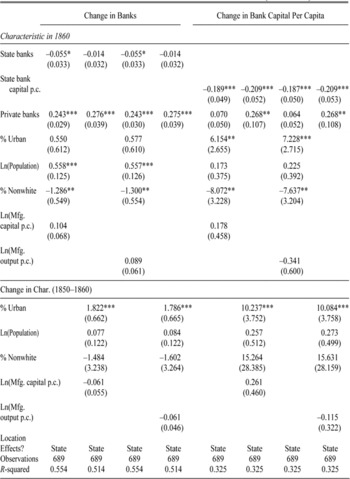
where the number of the initial number of private bankers (Priv_i,1860 ) measures the extent that the new national banks were formed by private bankers, and initial number of the state banks (State_i,1860 ) measures crowding out. X_i,1860 is the vector of county characteristics: the logarithm of county population and the fraction of population living in an urban area account for the demand for banking services, the fraction of nonwhite residents accounts for potential discrimination and racial conflict after the Civil War, manufacturing capital and output per capita account for industrial composition.Footnote ²¹ S_s denotes state-fixed effects that control for differential laws and regulations and e_i denotes the error term. In separate regressions, I include the change in the county-level variables over the 1850s instead of their level in 1860 to examine whether previous growth affects the change in banks.

Private bankers are treated as nonbanks for several reasons.Footnote ²² First, they were too small to have a large effect on manufacturing. A few private bankers took deposits and made loans, but most had little paid in capital and could not issue bank notes.Footnote ²³ When private bankers are included in place of ΔBanks_i,1863–66 , they are not significantly correlated with manufacturing activity. Second, they were not correlated with financial underdevelopment. Indeed, the highest ratios of private bankers to state banks were in free banking states. Finally, they started a sizeable portion of new national banks. By negating these “new banks,” much of the variation in the change in banks would be lost and the model would identify the coefficient on those places without private bankers. Moreover, as private bankers had already developed information capital and relationships in the local community, the effect of legislation might come from its ability to pull these individuals into the formal banking system.

The change in banks caused by the legislation was not correlated with manufacturing (Table 1). Neither the coefficients on manufacturing in 1860 nor the coefficients on growth during the 1850s are statistically or economically significant. For instance, a one-standard-deviation increase in manufacturing capital per capita (about 0.96) in 1860 would lead to about 0.01 new banks whereas a standard deviation higher in growth (about 0.61) during the 1850s would actually decrease the number of banks by 0.04. The shock to the banking system caused by the legislation thus was plausibly exogenous to manufacturing after controlling for the other county-level factors.

On the other hand, the number of private bankers in 1860 was a key factor for the sudden change in the number of banks. The more private bankers within a county the more new banks were established there during the mid-1860s, whereas more state banks almost seem to have a negative effect on bank entry. The rise in new national banks thus was driven by private bankers, and if anything, counties that did not have a bank in 1862 did not gain one by 1866.

Counties that started with larger populations gained banks, but not those counties that were growing fastest during the 1850s. For instance, a one-standard-deviation increase in population (about 0.81) in 1860 led to 0.45 more banks, but one-standard-deviation higher population growth (about 0.42) during the 1850s only led to about 0.032 additional banks. Counties that urbanized during the 1850s also seem to have attracted new banks. A one-standard-deviation increase in urbanization (about 0.077) would lead to 0.14 new banks. The difference is likely driven by the restrictive national bank capital requirements, as new banks could be established only in areas that had reached some population threshold. Because state and national banks had different required levels of capital, it is possible that some counties traded two small banks for one large bank. The rest of the table, therefore, replaces the change in the number of banks with the change in bank capital per person. The change is still not related to the 1860 level of manufacturing or the 1850–1860 growth in manufacturing, nor is it always statistically and significantly related to the number of private bankers either, suggesting that small private bankers did not create large national banks.

National Banking and County-Level Growth: 1860–1900

The identifying assumption of the dose model is that the treatment (i.e., the change in number of banks between 1863 and 1866) was exogenous. Table 1 indicates that the change in the number of banks was not correlated with manufacturing after controlling for the observable county-level characteristics, but in order for the causal effect to be plausibly identified there also must be no remaining correlation between omitted factors and the change in banks after controlling for the other variables. In the models that follow, I, therefore, include the previously tested characteristics, and also control for time-invariant factors that could have been driving both bank and manufacturing growth using county-fixed effects and county-specific linear time trends. While not available for 1850, the census tabulated the number of manufacturing establishments starting in 1860. I can normalize manufacturing capital and output by population and separately by the number of establishments. This additional normalization is important because the structural change in manufacturing after the Civil War was the result of a capital deepening.

TABLE 1

COUNTY-LEVEL DETERMINANTS OF BANK GROWTH (1863–1866)

* denotes significance at the 10 percent level.

** denotes significance at the 5 percent level.

*** denotes significance at the 1 percent level.

Notes:

The table presents the results of an ordinary least squares regression. The dependent variable is described in the column heading. Dollar values are deflated to 1860 using Officer (Reference Officer2008). Standard errors are provided in parentheses and clustered by state.

Sources:

See Data Section.

Each measure is modeled from 1860 to 1900 as a linear function of financial development and other county-level characteristics. The full model is as follows

(2) \begin{equation} Y_{i,t} = \alpha + \beta _1 \Delta Banks_i _{,1863 - 66} *post{\rm 1860}_t + \beta _2 nat_{i{\rm,}t - 1} + \beta _3 state_{i{\rm,}t - {\rm 1}} + \beta _4 X_{i,t - 1} + \tau _t + u_i + Trend_{i,t} + e_{i,t} \end{equation}

where post1860_t denotes an indicator variable that takes the value one when t is greater than 1860, Nat_{i,t − 1} denotes the number of national banks in the previous decade, X _{i,t − 1} denotes a vector that contains the logarithm of population, fraction urban, and fraction nonwhite, as well as an indicator variable that denotes whether the county had a reserve city, u_i denotes county-level fixed effects, τ_t denotes decade fixed effects, Trend_i,t denotes a vector of county-specific linear trends, and e_i,t denotes the error term which is clustered by county.Footnote ²⁴ Because the dose response model controls only for the endogeneity of banks entering during the 1860s, I follow studies such as Robert King and Ross Levine (Reference King and Levine1993) and use the initial number of banks rather than the contemporaneous value. The approach will reduce endogeneity, and any remaining bias should affect both bank types. The model can thus examine whether the effect of the two bank types differed but cannot measure the exact size of their causal effect on manufacturing.

TABLE 2

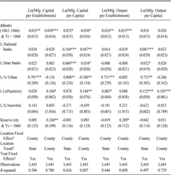
MEASURING NATIONAL BANKING'S EFFECT ON COUNTY-LEVEL MANUFACTURING (1860–1900)

* denotes significance at the 10 percent level.

** denotes significance at the 5 percent level.

*** denotes significance at the 1 percent level.

Notes:

The table presents the results of an OLS regression. The dependent variable is described in the column heading. The sample consists of decadal county-level observations from 1860 through 1900. Dollar values are deflated to 1860 using Officer (Reference Officer2008). Standard errors are provided in parentheses and are clustered by county.

Sources:

See Data Section.

The regression results in Table 2 indicate that the change in banking immediately after the National Banking Acts had a positive effect on manufacturing growth. The coefficient on is statistically significant for most of the manufacturing variables, but more so for the per establishment measures. A county gaining a bank between 1863 and 1866 is expected to have gained 3 percent more capital per capita, but 5 percent more capital per establishment. Alternatively, an extra initial bank would lead to an (insignificant) 2 percent more output per capita, but 3.5 percent more output per establishment. Putting these results into the context of the average growth between 1860 and 1900, the effect of gaining one bank during the period represented around 13 percent of per establishment growth and about 6 percent of per capita growth.Footnote ²⁵ Therefore, even without controlling for the positive influence that banking had through urbanization, the legislation accounts for a nontrivial portion of the period's growth and was particularly related to the structural changes taking place in the Manufacturing Belt.

While positively biased by endogeneity, banks after 1870 influenced manufacturing differently than the new banks in the 1860s. State and national banks generally have a positive and significant relationship with manufacturing capital and output per capita, but an insignificant negative relationship with the per establishment variables when a county-trend is included. The initial rise in banks thus might have accelerated the expansion of existing establishments while later banks helped new establishments enter the market. There is also weak evidence that the switch from state to national banks increased manufacturing growth. The coefficients on national banks are larger than those on state banks for the per capita measures, but are not consistently positively or negatively different for the per establishment measures.

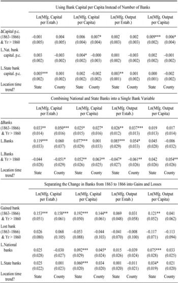
Seeking to clarify and expand on the analysis, I examine the data in four different ways in Table 3. The top panel replaces the number of banks with bank capital per capita. As state banks were often smaller than national banks, using the number of banks rather than bank capital could be one reason why the coefficients on state banks are smaller than national banks. While coefficient on the change in capital during the 1860s remains significant for the per capita measures, the coefficients on the capital of both national and state banks are generally insignificant. The pattern suggests that having access to banks is important regardless of the size of the bank during the postbellum period. This finding is not too surprising as the National Banking Acts and tax on state bank notes prevented entry in many rural areas. A county receiving its first bank regardless of how small would thus represent a tremendous boon to local industry, whereas additional banks would have less of an effect.

TABLE 3

ADDITIONAL TESTS OF NATIONAL BANKING'S EFFECT ON COUNTY-LEVEL MANUFACTURING (1860–1900)

* denotes significance at the 10 percent level.

** denotes significance at the 5 percent level.

*** denotes significance at the 1 percent level.

Notes:

The table presents the results of an OLS regression. The dependent variable is described in the column heading. The sample consists of decadal county-level observations from 1860 through 1900. Every regression includes county- and decade-fixed effects as well as the defined location trend and the county-level characteristics in all previous regression. Dollar values are deflated to 1860 using Officer (Reference Officer2008). Standard errors are provided in parentheses and are clustered by county.

Sources:

See Data Section.

The second panel tests whether the change in banking structure brought about by the National Banking Acts and the state bank note tax strengthened the connection between finance and growth. To do this, I aggregate state and national banks and test whether postbellum banks had a larger effect than antebellum banks. The coefficients show that banks had a stronger positive connection with per capita growth after 1870, but also a stronger negative one with per establishment growth. At the same time, the change in the number of banks in the 1860s remains positive and significant. In this way, the National Banking Acts and the state bank note tax may have enabled more growth than the previous banking system could have.

The third panel uses dummy variables to test whether bank losses during the 1860s hurt a county as much as gains helped it. The panel presents a more nuanced result: initial bank losses were not generally statistically or economically important and bank gains were much more important. Counties gaining a bank immediately after the Acts had 14.4 percent more manufacturing capital per capita than those that did not gain a bank, but a county losing a bank had (an insignificant) 0.4 percent less capital. The linear assumption of the model thus biased the coefficients on the change in banks towards zero. The final panel tests whether New England's developed financial system biased the coefficients by dropping the region out. Because the region's financial system was already composed of larger banks with high requirements, fewer changes occurred after the legislation passed. The coefficient on the change in banks remains generally positive and significant, but the coefficients on the number of state and national banks become less significant. The results suggest that the change in banks immediately around the legislation was responsible for the distribution of manufacturing growth and that the model is identified on the variation across the entire Manufacturing Belt instead of New England.Footnote ²⁶

Decomposing the County-Level Effect by Decade

The panel approach is helpful to control for unobserved heterogeneity, but only estimates the average effect of the change in the number of banks over the entire period. As the effect most likely varied over time, it is informative to run separate regressions for each decade. Because the repeated cross-section approach cannot include county-fixed effects, I have chosen to use the values of manufacturing, population, urbanization, and banks in 1860, effectively testing which initial characteristics best predicted manufacturing in each subsequent decade. Estimated separately for each decade, the regressions have the form

(3) \begin{equation} Y_{i,t} = \alpha + \beta _1 \Delta Banks_i _{,1863 - 66} + \beta _2 state_{i{\rm,1860}} + \beta _4 X_{i,1860} \beta _5 Y_{i,1860} + \beta _5 Y_{i,1860} + S_s + ei,t \end{equation}

where e_i,t is a vector of Huber-White standard errors and the other variables retain their previous definitions.

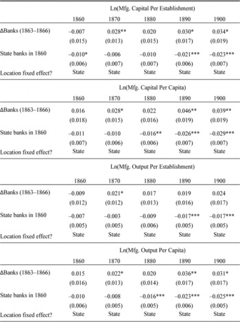
Table 4 illustrates that the effect of the change in the number of banks between 1863 and 1866 had a significant and generally increasing effect on manufacturing after 1870. The effect is strongest on manufacturing capital per capita and per establishment, but is also statistically significant for output per capita. A new bank gained between 1863 and 1866 increased manufacturing capital per capita 2.8 percent in 1870, 2.2 percent in 1880, 4.6 percent in 1890, and 3.9 percent in 1900, and manufacturing output per capita by 2.2 percent in 1870, 2 percent in 1880, 3.6 percent in 1890, and 3.1 percent in 1900. The effects account for about 8 percent of the period's average decennial growth. Alternatively, the number of state banks in 1860 was not significantly correlated with any measure of manufacturing in 1870 and the coefficients actually become more negative over time. The data thus indicate that the immediate changes brought about by the National Banking Acts had a larger and more persistent effect than the existing antebellum banking system.

TABLE 4

EXAMINING THE EFFECT OF THE CHANGE IN BANKING BY DECADE

* denotes significance at the 10 percent level.

** denotes significance at the 5 percent level.

*** denotes significance at the 1 percent level.

Notes:

The table presents the results of an OLS regression. The sample consists of county-level observations for the year specified by the column. The regression also contains the value of population, urbanization, and percent black in 1860. Starting in 1870 the model also controls for manufacturing in 1860 and whether the county contained a reserve city. Dollar values are deflated to 1860 using Officer (Reference Officer2008). Robust standard errors are provided in parentheses.

Sources:

See Data Section.

National Banking and Establishment-Level Growth: 1850–1880

The previous analysis suggests that the National Banking Acts drove manufacturing growth, but the county-level data only include certain aggregate measures. For instance, they contain the value of manufacturing capital, but not what type of capital it was or in which industry it was employed.Footnote ²⁷ I, therefore, use Atack and Bateman's establishment-level manufacturing sample (Reference Atack and Bateman1999) to pinpoint banking's effect on those characteristics (physical capital, steam power, and value added) that are associated with modern manufacturing. There are two drawbacks with the establishment-level data. First, the data do not contain the same establishments or counties each year so a fixed-effects estimator cannot be used. I thus include the level of ΔBanks _i,1863–66 in the regression to capture initial differences between areas.Footnote ²⁸ Second, the data do not contain each establishment's city and so establishments and banks must be matched by county. While the model cannot account for this type of measurement error, it should bias against finding a significant relationship between banks and manufacturing.

The full model is

(4) \begin{equation} Y_{j,i,t} = \alpha + \beta _1 \Delta Banks_i _{,1863 - 66} + \beta _2 \Delta Banks_{i{\rm,1863} - {\rm 66}} *Post1860t + \beta _3 Nat_{i,t - 1} + \beta _4 StateY_{i,t - 1} + \beta _5 X_{i,t - 1} + \beta _6 Z_{j,i,t} + \tau _t + S_s + I_j + S_s \times \tau _t + I_j \times \tau _t + e_{j,i,t} \end{equation}

where j denotes establishment, the vector Z_j,i,t contains a dummy if the establishment is in a city and dummy variables for its number of employees, I_j is fixed effects for three-digit industry codes, and all other variables retain their previous meanings.Footnote ²⁹ The interaction of state-fixed effects with decade effects capture location-specific institutional development, and the interaction of the industry-fixed effects with decade effects capture industrial development. It is helpful to point out that the model provides a lower-bound estimate of the effect of the National Banking Acts. First, some establishments might have been far away for the bank in their county. Second, any impact the legislation had on all the firms in an industry will be captured by the industry-year fixed effects. Third, the legislation's estimated effect grows over time in Table 4, but the establishment-level sample ends in 1880.

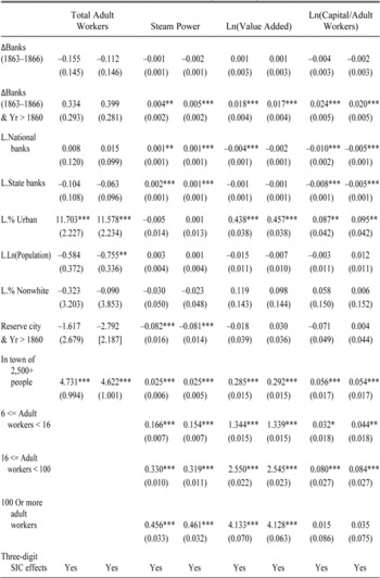
The sudden growth of banks during the 1860s assisted the structural and technological shifts associated with the establishment of the Manufacturing Belt. In Table 5, the change is positively and significantly correlated with capital per worker, the adoption of steam engines, and value added. An extra bank during the mid-1860s increased an establishment's capital to labor ratio by 2 percent, the probability of having steam power by 0.5 percent, and value added by 1.7 percent. The coefficients are small, but correspond to large proportions of the actual growth rates. For instance, the percent of firms with steam engines in the sample grew from 15 percent to 18 percent between 1860 and 1880. Therefore, the estimated effect of a new bank represented 17 percent of steam engine growth, 16 percent of the growth in value added, and nearly all of the growth in the capital to labor ratio over the period.

The change in banks was not statistically significantly correlated with the number of workers. For every extra bank gained during the 1860s, a firm would have 0.4 more workers. The fact the coefficient is not statistically significant or large is due to some banks following the Real Bills Doctrine which advocated short-term lending. Those banks that followed the tenants would not have provided long-term loans to construct a factory, and instead, were more likely to have helped firms mechanize their production processes through the purchase of smaller capital goods such as steam engines.

TABLE 5

MEASURING NATIONAL BANKING'S EFFECT ON ESTABLISHMENT-LEVEL MANUFACTURING (1850–1880)

* denotes significance at 10 percent level.

** denotes significance at 5 percent level.

*** denotes significance at 1 percent level.

Notes:

The table presents the results of an OLS regression. The sample consists of decadal firm-level observations from 1850 through 1880. The dependent variable is defined by the column heading. Dollar values are deflated to 1860 using Officer (Reference Officer2008). Robust standard errors are provided in parentheses.

Sources:

See Data Section.

The rest of the banking system does not have a consistently positive effect on manufacturers. Both state and national banks are significantly positively correlated with the adoption of steam power and significantly negatively correlated with capital per worker. The insignificant and often negative coefficients for national banks are the result of the limited number of postbellum observations, whereas those for state banks are the result of unstable banking during the antebellum period. The finding indicates that the changes brought about by the legislation had a new effect on the manufacturing sector.