Introduction
Modern communication requires smart antenna arrays with adaptive radiation characteristics. The synthesis of fourth-dimensional (4D) time-modulated antenna arrays have drawn an abundance of attention from the scientific community lately for its adaptive nature [Reference Rocca, Yang, Poli and Yang1]. To add a further degree of control to the already existing classic antenna arrays, fourth dimension “time” had been proposed for pattern synthesis [Reference Shanks and Bickmore2]. Excitation, phase, and the distance between elements used to be the three dimensions to control the radiation pattern of traditional array. This fourth dimension provided an advantage when the idea of regulating the array patterns by rapid switches had been introduced for electronic scanning [Reference Shanks3]. Due to its simple control by switching ON and OFF the antennas, the 4D arrays have emerged as an alternate to tapered phased arrays for achieving ultra-low sidelobe levels (SLLs) [Reference Kummer, Villeneuve, Fong and Terrio4]. However, the benefit comes with an intrinsic limitation of sideband pattern generation at infinite number of harmonic frequencies, typically thought of as power loss [Reference Bregains, Fondevila-Gomez, Franceschetti and Ares5]. Since then, so many efforts have been made to synthesize adequate average patterns at antenna operating frequency to reduce the spurious harmonic or sidebandradiation (SR) [Reference Yang, Gan and Qing6–Reference Zhu, Yang, Zheng and Nie8]. To further improve the efficiency of the array, simultaneous suppression of SLL and minimization of all higher-order sideband levels (SBLs) have been addressed [Reference Chakraborty, Ram and Mandal9, Reference Chakraborty, Ram and Mandal10]. An alternative strategy for direction finding has also emerged, one that utilizes the SBLs rather than suppressing them [Reference Tennant and Chambers11]. In addition, a novel electronic steering technique was put forth in [Reference Li, Yang, Chen and Nie12] by controlling the SRs. The 4D arrays had further been investigated to estimate the directions of arrival of target signal [Reference Gang, Yang and Nie13] by exploiting the beamforming capabilities of the harmonics [Reference Poli, Rocca, Oliveri and Massa14]. The harmonics have also been controlled by moving the phase center of the linear 4D arrays with suitable time schemes [Reference Chakraborty, Ram and Mandal15, Reference Chakraborty, Ram and Mandal16]. Novel methods to regulate the beam patterns have been made feasible by the design of proficient switching mechanisms utilizing pulse shifting [Reference Poli, Rocca, Manica and Massa17] and pulse splitting [Reference Poli, Moriyama and Rocca18]. Pattern generation of 4D arrays by attenuating [Reference Poddar, Paul, Chakraborty, Ram and Mandal19] or exploiting [Reference Chakraborty, Ram and Mandal20] the SRs has been reported for multifunction radars [Reference Chakraborty, Saxena, Verma, Juyal, Gupta, Singh, Ram and Mandal21, Reference Chakraborty, Ram and Mandal22]. Controlling a sideband by progressive phase shifted switching [Reference Tong and Tennant23], or multiple higher-order sidebands by optimal phase shifting [Reference Chakraborty, Ram and Mandal24, Reference Chakraborty, Ram and Mandal25] have opened up the possibilities for multipoint communication. Due to its adaptiveness, 4D arrays exhibit multifold prospect compared to its traditional counterparts if the sideband power is properly controlled [Reference Chakraborty, Singh, Gupta, Ram and Mandal26]. Automatic beam steerable 4D arrays with single and multiple steered beams have also come into the picture by channelizing the sideband power in desired directions [Reference Maneiro-Catoira, Brégains, García-Naya and Castedo27, Reference Ram and Mandal28]. The 4D planar arrays have further been proposed for harmonic beamforming [Reference Ma, Miao, Li and Wu29], and for directional modulation purposes by controlling its phase time sequences [Reference Li, Chen and Yang30]. For more advanced applications like monopulse radars, sum-difference beams have also been generated using convex optimization methods [Reference Dong, Li, Tan, Hu and Jiang31]. Due to its efficient beamforming capabilities, 4D arrays have also been extensively investigated for physical secure communication [Reference Chen, Yang, Chen, Qu and Hu32, Reference Qu, Chen, Long, Chen, Qu, Hu and Yang33]. Multi-tone harmonics of 4D arrays have also been explored for Wireless Information and Power Transfer (WIPT) [Reference Suneel Varma, Ram and Arun Kumar34]. The harmonics have been used advantageously for steerable energy patterns [Reference Reyna, Panduro, Romero, Villanueva, Rivera and Méndez35]. Different structures and combinations such as spiral [Reference Reyna, Panduro, Méndez and Romero36], circular and concentric circular [Reference Medina, Reyna, Panduro and Elizarraras37, Reference Ram, Kar and Mandal38] and concentric ring shaped 4D antenna arrays [Reference Reyna Maldonado, Panduro, Del Rio Bocio and Mendez39] have also been tested. Further, the concept had also been applied for Unmanned aerial vehicles and 5 G communications [Reference Jiménez, Reyna, Panduro, Del Rio, Ram and Balderas40, Reference Maldonado, Maldonado, Balderas and Panduro41]. In this way, time-modulation has become a serious research interest for the modern-world communication [Reference Varma, Ram and Arun Kumar42].
This article contributes to the competitive world of antenna array research by aiming to design an efficient beamforming array with optimal radiation properties. The efficient analysis of 4D linear arrays is discussed in this study to generate less-attenuating radiation patterns with sequentially suppressed sidelobe and sidebands. In this regard, an idea of splitting pulses while maintaining an optimal total switch ON duration is designed as an additional level of freedom for beamforming. In order to improve the overall radiation efficiencies of the array, the SLL and SBLs at the fundamental and harmonic frequencies are minimized. A set of linear arrays containing 16, 24, and 30 elements are investigated by proposing unique splitting pulse switching sequences for each array. Pulse splitting in between optimal modulation period provides an extra edge of control over the undesired radiations and power wasted in higher-order harmonics. The optimal pulse splitting schemes are designed by a wavelet-mutation based heuristic method by taking multiple objectives in a single-objective cost function as minimization problem. The outcomes are compared with other state of the art works, and a detailed statistical analysis is also reported to show the efficacies of the method.
The idea and methods proposed here have numerous benefits over other contemporary methods pertaining to antenna arrays employed for complex beamforming applications. The methodologies proposed in this research, stands out from other contemporary research works, and the advantages or benefits of the proposed methodologies are as follows:
Methodologies: First of all, optimal splitting pulse sequences are designed for efficient beamforming purposes. Second, ultra-low SLLs have been targeted by channelizing maximum power to the main beams. Then, unwanted SBLs have been suppressed to reduce the power wastage and improve efficiencies. This automatically mitigates the unwanted interferences coming from non-desired directions. In addition to that, all the higher sidebands are also lowered and up to 20 SBLs have been reported. For the overall optimization process, wavelet mutation is implemented to balance the exploration and exploitation stages. It is further compared with other hybrid and traditional mutation processes in terms of outcomes of the problem in hand. Finally, simultaneous mitigation of SLLs and SBLs have been proposed by implementing a single beamforming network (BFN).
Benefits: The array is targeted to perform both SLL and SBL reduction simultaneously compared to only SLL reduction or only SBL reduction aimed in most of the other research works. The modulation periods are managed and controlled with optimally splitting pulses in comparison to optimized time duration only reported in most other literature. The splitting pulse concept is also beneficial for BFNs as the optimal radiation properties can be implemented with only one BFN instead of different BFNs used to control the main beam and side beams separately reported in other works. Thus, only one BFN is sufficient here for both SLL and SBL reduction and simplifies the implementational task compared to its counterparts. As the proposed work is free from BFN related implementational complexities, it also provides an adaptive, robust, and efficient method of beamforming compared to the conventional ones. The performance of the beamforming arrays has also improved to a large extent due to wavelet mutation-based heuristic optimization methods employed to determine the optimal duration and ON-time instants.
The sequence of the remaining material is as follows: The design insights and the switching concept of 4D arrays are outlined in Section 2. Section 3 briefly describes a wavelet-based heuristic method. In Section 4, the results are examined with comparative and comprehensive analysis. The concluding remarks are laid out in Section 5.
Theory and design equations
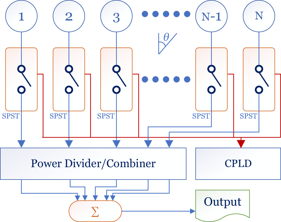
The simplified beamforming network (BFN) of a 4D linear array consists of N isotropic radiators attached through rapid radio-frequency (RF) switches, is shown in Fig. 1. The corresponding array factor (AF) without any loss of generality can be given as [Reference Rocca, Yang, Poli and Yang1]
 \begin{equation}AF(\theta ,t) = e^{j(2\pi {f_0})t}\sum\limits_{n = 1}^{N} {I_n}{U_n}(t){e\,^{jk(n - 1)dcos\theta }}\end{equation}
N-element fourth-dimensional (4D) linear antenna array with beamforming network (BFN).

where,  ${I_n}$ represents the excitation of the nth antenna,
 $k$ is the propagation constant,
 $d$ is considered as uniform element spacing,
 $\theta $ is the angle of impinging signals,
 ${f_0}$ is the central frequency with
 ${T_0}$ being the fundamental period, and
 ${U_n}\left( t \right)$ is the time modulation function.
Due to the periodic nature,  ${U_n}\left( t \right)$ may be given as [Reference Rocca, Yang, Poli and Yang1]
 \begin{equation}{U_n}\left( t \right) = \mathop \sum \limits_{m = - \infty }^\infty {a_{mn}}{e^{jm\left( {2\pi {f_p}} \right)t}}{ }\end{equation}
The Fourier term of excitation ( ${a_{mn}}$) for a particular radiating antenna (nth) at pre-defined harmonic frequencies (mth), automatically created due to modulation, can be given as [Reference Rocca, Yang, Poli and Yang1]
 \begin{equation}{a_{mn}} = \frac{1}{{{T_p}}} \int \limits_0^{{T_p}} {U_n}\left( t \right){e^{ - jm\left( {2\pi {f_p}} \right)t}}{ }dt\end{equation}
Thus, the AF for uniformly excited ( ${{\text{I}}_{\text{n}}}{\text{ = 1}}$) 4D linear array may be expressed as [Reference Chakraborty, Ram and Mandal9]
 \begin{equation}AF\left( {\theta ,t} \right) = \mathop \sum \limits_{m = - \infty }^\infty \mathop \sum \limits_{n = 1}^N {a_{mn}}\left\{ {{e^{jk\left( {n - 1} \right)dcos\theta }}} \right\}{e^{j2\pi \left( {{f_0} + m{f_p}} \right)t}}\end{equation}
The corresponding AF for mth order frequencies may be simplified as [Reference Chakraborty, Ram and Mandal9]
 \begin{equation}A{F_m}\left( {\theta ,t} \right) = {e^{j2\pi \left( {{f_0} + m{f_p}} \right)t}}\mathop \sum \limits_{n = 1}^N {a_{mn}}{e^{jk\left( {n - 1} \right)dcos\theta }}\end{equation}
The central pattern is generated at m = 0, and SRs are placed at multiple of modulation frequencies such as m = ± 1, ± 2, ± 3, …, ±∞. The directivity of the 4D array is [Reference Chakraborty, Ram and Mandal10]
 \begin{equation}Dir = \frac{{{{\left| {A{F_0}\left( {{\theta _0},{\phi _0}} \right)} \right|}^2}}}{{\frac{1}{{4\pi }}\mathop \sum \nolimits_{m = - \infty }^\infty \mathop \int \nolimits_0^{2\pi } \mathop \int \nolimits_0^\pi {{\left| {A{F_m}\left( {\theta ,\phi } \right)} \right|}^2}sin\theta d\theta d\phi }}\end{equation}
where the central pattern  $\left( {m = 0} \right)$ has placed at
 $\theta = {\theta _0}$,
 $\phi = {\phi _0}$ in a three-dimensional plane, and
 $A{F_m}\left( {\theta ,\phi } \right)$ denotes the AF pattern at
 $m$th harmonics.
Basic time modulation scheme
Considering its periodic character, the switching module  ${U_n}\left( t \right)$ may be derived in different ways for different switching sequences. In order to achieve beamforming patterns, the method suggested here involves splitting and shifting of each separable pulses within a modulation period (
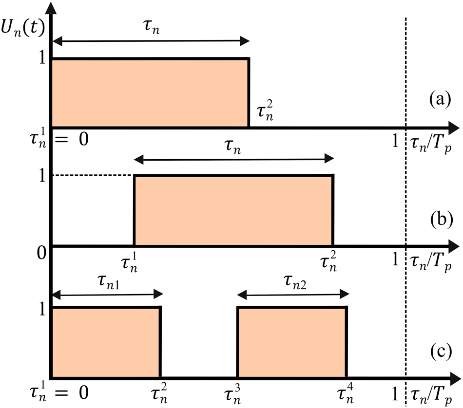
 ${T_p}$). Pulse splitting and shifted pulse, along with a general ON-OFF rectangular time scheme is shown in Fig. 2.
 ${U_n}\left( t \right)$ for the general one is expressed as [Reference Chakraborty, Ram and Mandal9]:
 \begin{equation}{U_n}\left( t \right) = \left\{ {\begin{array}{lc}
1,& 0 \leq \tau _n^1 \leq t \leq \tau _n^2 \leq {T_p} \\
0,& otherwise
\end{array}} \right.\end{equation}
(a) simple pulse, (b) shifted pulse, (c) sub-sectioned pulse (pulse splitting).

The ON-time for nth element is specified as  ${\tau _n}$ within the modulation time
 ${T_p}$
 $\left( {0 \leq {\tau _n} \leq {T_p}} \right)$, and normalized ON-time is
 $\left\{ {{\tau _n}/{T_p}} \right\}$. The element is turned ON initially (without shifting) as shown in Fig. 2(a) and the shifted pulse is given in Fig. 2(b). The shifted pulse starts at
 $\tau _n^1$ and closes at
 $\tau _n^2$ with a normalized ON-time
 $\left\{ {\left( {\tau _n^2 - \tau _n^1} \right)/{T_p}} \right\}$. Taking uniform excitations
 $\left( {{I_n} = 1} \right)$ for each element of the array
 $\left( {n = 1,2,3,\ldots N} \right)$,
 ${a_{mn}}$ can be determined as [Reference Chakraborty, Ram and Mandal9]
 \begin{align}
{a_{mn}} &= \frac{1}{{{T_p}}}\mathop \int \limits_{\tau _n^1}^{\tau _n^2} {U_n}\left( t \right){e^{ - jm\left( {2{{\pi }}{f_p}} \right)t}}\,dt \nonumber\\
& = \frac{1}{{{T_p}}}\frac{1}{{\left\{ { - jm\left( {2\pi {f_p}} \right)} \right\}}}\left[ {{e^{ - jm\left( {2\pi {f_p}} \right)t}}} \right]_{\tau _n^1}^{\tau _n^2} \nonumber\\
& = \frac{1}{{{T_p}}}\frac{1}{{\left\{ { - jm\left( {2\pi {f_p}} \right)} \right\}}}\left[ {{e^{ - jm\left( {2\pi {f_p}} \right)\tau _n^2}} - {e^{ - jm\left( {2\pi {f_p}} \right)\tau _n^1}}} \right] \nonumber\\
& = \frac{1}{{{T_p}}}\frac{j}{{\left\{ {m\left( {2\pi {f_p}} \right)} \right\}}}\left[ {{e^{ - jm\left( {2\pi {f_p}} \right)\tau _n^1}}\left\{ {{e^{ - jm\left( {2\pi {f_p}} \right)\left( {\tau _n^2 - \tau _n^1} \right)}} - 1} \right\}} \right] \nonumber\\
& = \frac{1}{{(1/{f_p})}}\frac{j}{{\left\{ {m\left( {2\pi {f_p}} \right)} \right\}}} \left[ {e^{ - jm\left( {2\pi {f_p}} \right){{\tau }}_n^1}} \right.\nonumber\\
&\quad \left. \times \left\{ {{e^{ - jm\pi {f_p}\left( {{{\tau }}_n^2 - {{\tau }}_n^1} \right)}}\left( {{e^{ - jm\pi {f_p}\left( {\tau _n^2 - \tau _n^1} \right)}} - {e^{jm\pi {f_p}\left( {\tau _n^2 - \tau _n^1} \right)}}} \right)} \right\} \right] \nonumber\\
& = \frac{j}{{2\pi m}}{e^{ - jm\left( {2\pi {f_p}} \right)\tau _n^1}}\,{e^{ - jm\pi {f_p}\left( {\tau _n^2 - \tau _n^1} \right)}}\left[ { - 2jsin\left\{ {m{{\pi }}{f_p}\left( {\tau _n^2 - \tau _n^1} \right)} \right\}} \right] \nonumber\\
& = \frac{{j\left( { - 2j} \right)}}{{2\pi m}}{e^{ - jm\pi {f_p}\left( {2\tau _n^1 + \tau _n^2 - \tau _n^1} \right)}}\left[ {sin\left\{ {m\pi {f_p}\left( {\tau _n^2 - \tau _n^1} \right)} \right\}} \right] \nonumber\\
& = \frac{1}{{m\pi }}\left[ {sin\left\{ {m\pi {f_p}\left( {\tau _n^2 - \tau _n^1} \right)} \right\}} \right]\,{e^{ - jm\pi {f_p}\left( {\tau _n^1 + \tau _n^2} \right)}} \nonumber\\
& = {f_p}\left( {\tau _n^2 - \tau _n^1} \right)\frac{{\left[ {sin\left\{ {m\pi {f_p}\left( {\tau _n^2 - \tau _n^1} \right)} \right\}} \right]}}{{\left[ {m\pi {f_p}\left( {\tau _n^2 - \tau _n^1} \right)} \right]}}{e^{ - jm\pi {f_p}\left( {\tau _n^1 + \tau _n^2} \right)}}
\end{align}
 \begin{equation} = \frac{{\left( {\tau _n^2 - \tau _n^1} \right)}}{{{T_p}}}{ }\left[ {sinc\left\{ {m\pi {f_p}\left( {\tau _n^2 - \tau _n^1} \right)} \right\}} \right]\,{e^{ - jm\pi {f_p}\left( {\tau _n^1 + \tau _n^2} \right)}}\end{equation}
Equation (9) represents the pulse shifted scheme of Fig. 2(b).
Switching with splitting pulses
To address a wide range of purposes, various switching mechanisms may be devised. Towards this purpose, a sub-sectioned splitting pulse scheme for nth element is given in Fig. 2(c), where the ON-time of each antenna is split up into sub-sections having an OFF-time in between. The nth element is turned ON at  $\tau _n^1$ (
 $\tau _n^1 = 0$) and stays ON up to
 $\tau _n^2$ creating an ON-duration of
 ${\tau _{n1}}$ (
 $ = \tau _n^2 - \tau _n^1$). Then, the antenna is turned OFF and stays OFF from
 $\tau _n^2$ to
 $\tau _n^3$ before going into the ON-state again for a duration of
 ${\tau _{n2}}$ (
 $ = \tau _n^4 - \tau _n^3$). The modulation function
 ${U_n}\left( t \right)$ of the sub-pulse can be given as
 \begin{equation}{U_n}(t) = \left\{ \begin{gathered}
1,\,\tau _n^1 \leq t \leq \tau _n^2 \leq {T_p}\,{\text{where}}\,\tau _n^1 = 0 \hfill \\
1,\,\,\tau _n^3 \leq t \leq \tau _n^4 \leq {T_p}{\text{ where }}\tau _n^1 \lt \tau _n^3 \hfill \\
0,\,{\text{otherwise }} \hfill \\
\end{gathered} \right.\end{equation}
The  ${a_{mn}}$ for the sub-sectioned pulses may be expressed as
 \begin{align}
{a_{mn}} &= \frac{{\left( {\tau _n^2 - \tau _n^1} \right)}}{{{T_p}}}\left[ {sinc\left\{ {m\pi {f_p}\left( {\tau _n^2 - \tau _n^1} \right)} \right\}} \right]{e^{ - jm\pi {f_p}\left( {\tau _n^1 + \tau _n^2} \right)}} \nonumber\\
&\quad + \frac{{\left( {\tau _n^4 - \tau _n^3} \right)}}{{{T_p}}}\,\left[ {sinc\left\{ {m\pi {f_p}\left( {\tau _n^4 - \tau _n^3} \right)} \right\}} \right]\,{e^{ - jm\pi {f_p}\left( {\tau _n^3 + \tau _n^4} \right)}}\end{align}
These derivations indicate that modified switching schemes offer higher degrees of freedom (DoF) than the standard ON-OFF sequence. This added DoF can be effectively utilized by manipulating the harmonics without altering the central beam pattern. Splitting each time period into multiple time steps with different switch-ON instants, optimized switch-ON and switch-OFF intervals can be summarized from equation (11) as follows:
 \begin{align}a_{mn}^r = \mathop \sum \limits_{r = 1}^s \frac{{\left( {\tau _n^{r + 1} - \tau _n^r} \right)}}{{{T_p}}}{ }\left[ {sinc\left\{ {m\pi {f_p}\left( {\tau _n^{r + 1} - \tau _n^r} \right)} \right\}} \right]\,{e^{ - jm\pi {f_p}\left( {\tau _n^r + \tau _n^{r + 1}} \right)}}\nonumber\\
\end{align}
Equation (12) represents splitting pulse shown in Fig. 2(c). Here,  $r = 1$ represents only the shifting of pulses for each antenna, and
 $r \gt 1$ can be accounted for splitting of pulses into sub sections and shifting them with optimal time intervals between each sub-sectioned pulse. By taking
 $r = 0$, the generalized expression of
 ${a_{mn}}$ for the mth harmonic at
 $m = 0$ can also be found from eqn. (12) as:
 \begin{equation}{a_{mn}} = \frac{{{\tau _n}}}{{{T_p}}}\left\{ {sinc\left( {m\pi {f_p}{\tau _n}} \right)} \right\}\,{e^{ - jm\pi {f_p}\left( {{\tau _n}} \right)}}\end{equation}
where,  ${\tau _n} = \left( {\tau _n^2 - \tau _n^1} \right)$ and the excitation coefficient of central pattern (
 $m = 0$) is given as:
 ${a_{mn}} = \{ {\tau _n}/{T_p}\} $. This indicates that the central beam is not altered with splitting and shifted pulse, as it is mathematically related only to the switch-ON time of the antennas. But the SR patterns depend on switch-ON instants as well as the switch-ON time periods for beamforming.
Design equation for optimization
Therefore, it turns out that the sideband power losses can be suppressed by properly adjusting the values of the static excitations, as well as the durations and starting instants of the ON-time pulses. To further reduce the optimization burden and the control parameters, uniform amplitude is taken in to account. Then, using an iterative heuristic optimization approach, the switch-ON instants and the switch-ON time periods are tuned with the goal of minimizing the SLLs and SBLs of a specific cost function. Reduction in sideband power losses and interference rejection of the central pattern for beamforming may be targeted as a minimization problem. By optimizing the normalized ON-time periods of each antenna, the SLL of the main beam can be lowered. Sideband radiation power may be is averaged over the whole angular region by optimally shifting and splitting the ON-time pulses. The CF for the overall optimization process is designed as
 \begin{align}{\text{CF}} &= {\left. {\{ {\psi ^{SLL\left( i \right)}}\left( {{\tau _n}} \right)\} } \right|_{{f_0} \pm m{f_p}\,\left( {m = 0} \right)}} \nonumber\\
&\quad + {\left. {\{ {\psi ^{SBL\left( i \right)}}\left( {{\tau _n},\tau _n^r} \right)\} } \right|_{{f_0} \pm m{f_p}\,\left( {m = 1,2,\,3,...,\infty } \right)}}\end{align}
where,  ${{{\psi }}^{{\text{SLL}}\left( i \right)}} = {\text{H}}\left[ {{\text{SL}}{{\text{L}}_{{\text{REF}}}} - {\text{SL}}{{\text{L}}_{{\text{OBS}}}}} \right]\left( {{\left| {{\text{SL}}{{\text{L}}_{{\text{REF}}}} - {\text{SL}}{{\text{L}}_{{\text{OBS}}}}} \right|}^2}/\right.$
 $ \left. {{\left| {{\text{SL}}{{\text{L}}_{{\text{REF}}}}} \right|}^2} \right)$,
 ${\text{SL}}{{\text{L}}_{{\text{REF}}}}$ and
 ${\text{SL}}{{\text{L}}_{{\text{OBS}}}}$ are the reference and observed SLLs respectively,
 ${\psi ^{SBL\left( i \right)}}$ represents the minimization of all the higher SBLs, H[.] is the Heaviside unit step function, and
 $i$ denotes the number of evolutions performed for the optimization process.
Heuristic optimization technique
Heuristic optimization algorithms are robust and adaptive in nature, and combines the exploration and exploitation strategies to investigate a solution space for optimum solutions [Reference Del Ser, Osaba, Molina, Yang, Salcedo-Sanz, Camacho, Das, PN, CA and Herrera43]. Evolutionary optimizations have evolved as population-based metaheuristic search method motivated by natural phenomena for solving various real-world engineering problems, especially in the area of antenna array synthesis [Reference Sharaqa and Dib44–Reference Ram, Mandal, Kar and Ghoshal46].
Standard particle swarm optimization
Particle swarm optimization (PSO) is a well-known, robust, and stochastic optimization tool based on the movement and intelligence of swarms [Reference Robinson and Rahmat-Samii47]. Standard PSO (SPSO) has been demonstrated to be beneficial for a number of fields for optimizing challenging multidimensional discontinuous problems especially antenna design and pattern synthesis in electromagnetics [Reference Robinson and Rahmat-Samii47]. SPSO models the sociological behaviour of bird flocking and fish schooling in multi-dimensional space. It takes into account a number of particles that collectively constitute a swarm. Each particle in the swarm traverses the solution space looking for the global best ( ${g_{best}}$) while considering their individual or personal best (
 ${p_{best}}$) also at each iteration. The process continues by minimizing the distance between the present position of the particle and its personal best (
 ${p_{best}}$), as well as, the distance between the present position of a particle and the global best (
 ${g_{best}}$) as per the following equations:
 \begin{align} v_j^p\left( {i + 1} \right) &= {C_F}.\left\{ w.v_j^p\left( i \right) + {\varphi _1}.ran{d_1}.\left( {{p_{best}}_j^p - s_j^p\left( i \right)} \right) \right. \nonumber\\
&\quad \left.+ {\varphi _2}.ran{d_2}.\left( {{g_{best}}_j - s_j^p\left( i \right)} \right) \right\}\end{align}
 \begin{equation}s_j^p\left( {i + 1} \right) = s_j^p\left( i \right) + v_j^p\left( {i + 1} \right)\end{equation}
Here, eqn. (15) and (16) are the velocity updating and position updating equations, respectively. The  $v_j^p\left( i \right)$ is the velocity at ith iteration, with
 $p = 1,2, \ldots ,\gamma $ being the number of particles in the swarm and
 $j = 1,2, \ldots ,\kappa $ being the dimension of the particle. The
 ${\varphi _1}$ and
 ${\varphi _2}$ in eqn. (15) represents the social and cognitive acceleration constants;
 $w$ is the inertia weight factor;
 $s_j^p\left( i \right)$ is the present position of a particle in the search space;
 $ran{d_1}$ and
 $ran{d_2}$ are the random numbers in between 0 and 1. The
 ${C_F}$ stands for the constriction factor which affects the stability analysis by ensuring no premature convergence, and mathematically represented in terms of acceleration constants as [Reference Ling, Iu, Chan, Lam, Yeung and Leung48]:
 \begin{equation}{C_F} = \frac{2}{{\left| {2 - \varphi - \sqrt {{\varphi ^2} - 4\varphi } } \right|}}\end{equation}
Here,  $\varphi = {\varphi _1} + {\varphi _2}$ and
 $\varphi \gt 4$.
Hybrid PSO with wavelet mutation
Towards the near-optimal solution, SPSO typically encounters issues related to velocity updating despite working effectively in the beginning. If the particle’s present state is coinciding with global best position, the particle will only move from its present state if its inertia weight and velocity are different from zero. The particles will stop moving if their velocities are near to zero, and they will catch up with the  ${g_{best}}$, which may result in an early convergence and prevent future development by being stagnant at a particular position. To balance the global and local explorations, the inertia weight factor
 $w$ may be chosen dynamically as [Reference Ling, Iu, Chan, Lam, Yeung and Leung48]:
 \begin{equation}w = \left[ {{w_{max}} - \left\{ {\left( {\frac{{{w_{max}} - {w_{min}}}}{{{i_{max}}}}} \right)*i} \right\}} \right]\end{equation}
Here,  ${i_{max}}$ presents the maximum iterations; and
 $w$ is varied between the upper (
 ${w_{max}}$) and lower (
 ${w_{min}}$) limits in a range of [1,0.4]. The hybrid PSO (HPSO) is proposed by integrating the mutation operation of genetic algorithms [Reference Weile and Michielssen49] to break through the stagnation stages of SPSO as following:
 \begin{equation}mut\left( {{s_j}} \right) = \left\{ {\begin{array}{*{20}{c}}
{({s_j} - k),\,r \lt 0} \\
{({s_j} + k),\,r \geq 0}
\end{array}} \right.\end{equation}
Here,  ${s_j}$ is the randomly chosen element of the particle from the swarm; r is a random number in between—1 and 1;
 $k$ is randomly generated within
 $\left[ {{\text{0,0}}{\text{.1}}*\left( {par_{max}^j - par_{min}^j} \right)} \right]$; where
 $par_{min}^j$ and
 $par_{max}^j$ are the lower and upper limits of each particle, respectively. However, the mutation space in HPSO is limited by
 $k$. It might not be the best approach to always fix the size of the mutation space during the search. Rather, a dynamic mutation process that dynamically shrinks the mutation space along the search may be integrated. To implement this, a wavelet mutation (WM) approach is integrated with HPSO.
Basic wavelet theory
The translating and dilating oscillatory properties of some specific seismic signal may be modelled in to a continuous function  $\psi \left( x \right)$ generally called as “Morlet” or “mother wavelet” if it satisfies the following properties [Reference Ling, Iu, Chan, Lam, Yeung and Leung48]:
 \begin{equation}{\text{Property 1}}:\mathop \int \limits_{ - \infty }^{ + \infty } \psi \left( x \right)dx = 0\end{equation}
 \begin{equation}{\text{Property 2:}}\mathop \int \limits_{ - \infty }^{ + \infty } {\left| {\psi \left( x \right)} \right|^2} \lt \infty \end{equation}
It means that the total momentum of  $\psi \left( x \right)$ is equal to zero, or the positive and negative momentum of
 $\psi \left( x \right)$ is equal to each other. Also, the continuous function
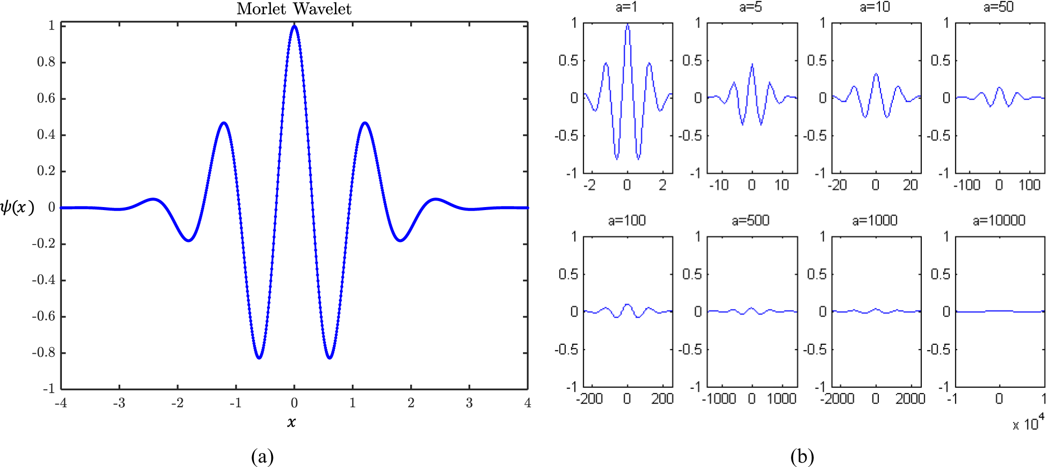
 $\psi \left( x \right)$ can be said finite and bounded. A typical “Morlet wavelet” is shown in Fig. 3(a), and may be represented mathematically as [Reference Ling, Iu, Chan, Lam, Yeung and Leung48]
 \begin{equation}\psi \left( x \right) = {e^{ - {x^2}/2}}\,{\text{cos}}\left( {5x} \right)\end{equation}
(a) morlet wavelet, (b) characteristics of morlet wavelet for different dilating parameter values [Reference Ling, Iu, Chan, Lam, Yeung and Leung48].

For controlling the magnitude and position of the “Morlet wavelet”, the continuous function  $\psi \left( x \right)$ is extended as [Reference Ling, Iu, Chan, Lam, Yeung and Leung48]
 \begin{equation}{\psi _{a,b}}\left( x \right) = \frac{1}{{\sqrt a }}\psi \left( {\frac{{x - b}}{a}} \right)\end{equation}
Here,  $a$ and
 $b$ are the dilating and translating parameters, respectively. With
 $b = 0$, the amplitude scaled version of
 $\psi \left( x \right)$ can be derived. The scaled
 ${\psi _{a,0}}\left( x \right)$ for the different dilation properties are shown in Fig. 3(b), and can be represented mathematically as [Reference Ling, Iu, Chan, Lam, Yeung and Leung48]
 \begin{equation}{\psi _{a,0}}\left( x \right) = \frac{1}{{\sqrt a }}\psi \left( {\frac{x}{a}} \right)\end{equation}
The amplitude can be scaled down by increasing the value of dilating parameter, and this property is utilized in the mutation process to enhance the search performance of the algorithm [Reference Ling, Iu, Chan, Lam, Yeung and Leung48].
Operation of the WM
The wavelet-based mutation exhibits fine tuning by giving every element particle of the swarm a chance to mutate within a user-defined mutation probability  ${P_m} \in {\text{[0,1]}}$. Thus, if the pth particle is chosen and the element particle of the swarm
 $x_j^p\left( i \right)$ is selected randomly for mutation, the resultant particle can be given as [Reference Ling, Iu, Chan, Lam, Yeung and Leung48]
 \begin{equation}\bar x_j^p(i) = \left\{ {\begin{array}{*{20}{c}}
{x_j^p\left( i \right) + \sigma .\left[ {par_{max}^j - x_j^p\left( i \right)} \right]\,if\,\sigma \gt 0} \\
{x_j^p\left( i \right) + \sigma .\left[ {x_j^p\left( i \right) - par_{min}^j} \right]\,if\,\sigma \leq 0}
\end{array}} \right.\end{equation}
Here,  $\sigma = {\psi _{a,0}}\left( x \right) = \frac{1}{{\sqrt a }}\psi \left( {\frac{x}{a}} \right)$ and
 $\psi \left( x \right) = {e^{\left( { - \frac{{{x^2}}}{2}} \right)}}cos\left( {5x} \right)$. So, dilating parameter (
 $\sigma $) becomes
 \begin{equation}\sigma = \frac{1}{{\sqrt a }}{e^{\left\{ {{{\left( { - \frac{x}{a}} \right)}^2}/2} \right\}}}cos\left\{ {5\left( {\frac{x}{a}} \right)} \right\}\end{equation}
When  $\sigma $ is positive (
 $\sigma \gt 0$) and approaching to + 1, the mutated particle element tends to have the maximum of
 $x_j^p\left( i \right)$. On the other hand, when
 $\sigma $ is negative (
 $\sigma \leq 0$) and approaching to—1, it has the minimum value of
 $x_j^p\left( i \right)$. The larger the value of
 $\left| \sigma \right|$, the searching space for fine tuning is large and vice-versa. According to the properties of mother wavelet, the sum of the positive and negative
 $\sigma $ are equal when the sample is large. Thus, the positive and negative mutation is equal which provides a better solution stability. Further, the dilating parameter (
 $a$) can be expressed as
 \begin{equation}a = {e^{ - ln\left( g \right)*{{\left( {1 - \frac{i}{K}} \right)}^{{\xi _{wm}}}} + ln\left( g \right)}}\end{equation}
The dilating parameter ( $a$) varies with
 $\left( {\frac{i}{K}} \right)$, where
 $i$ stands for current evolution and
 $K$ is the total number of evolutions. The monotonically increasing shape parameter is denoted by
 ${\xi _{wm}}$ and
 $g$ is the upper limit of the dilating parameter
 $a$ [1,10000]. In HPSOWM, an optimal balance is projected between the exploitation of previously sampled regions in the search space and the exploration of new regions. An updated swarm is created after the WM operation, and the swarm will follow the same process over and over again until the termination criteria is reached.
Numerical data and analysis
This upcoming section discusses the numerical outcomes by a thorough examination of 16, 24, 30-element 4D linear arrays that have been developed, where the required objectives are achieved by combining a soft computing method with pulse control methodologies. The operational frequency (f0) of the 4D linear arrays is 3 GHz with a modulation frequency (fp) of 1 MHz. The properties of isophoric (In = 1) 16, 24, 30-element 4D linear arrays are: Peak SLLs = —13.15 dB,—13.21 dB,—13.24 dB; 3 dB beamwidths (HPBWs) = 6.48˚, 4.32˚, 3.60˚; beamwidth within the first nulls (FNBWs) = 14.4˚, 9.72˚, 7.56˚; and directivities = 12.04 dB, 13.80 dB, 14.77 dB; respectively. All the simulations are performed with MATLAB.
Beamforming with splitting pulses
An analysis of 4D linear arrays is investigated here in order to produce less-attenuating radiating beam patterns with sequentially lowered SLLs and SBLs. First, high-directive beamforming arrays with ultra-low SLLs are targeted, and then all the higher SBLs are minimized to reduce unwanted power loss. The aim is to design the optimal switching schemes by splitting the pulses within the pre-specified modulation period such that the SLL and the SBLs can be minimized to reduce the unwanted interference and the undesired power radiation in higher harmonics, respectively. The possible application of beamforming array is for directive point-to-point communication systems.
Beamforming with 16-element array
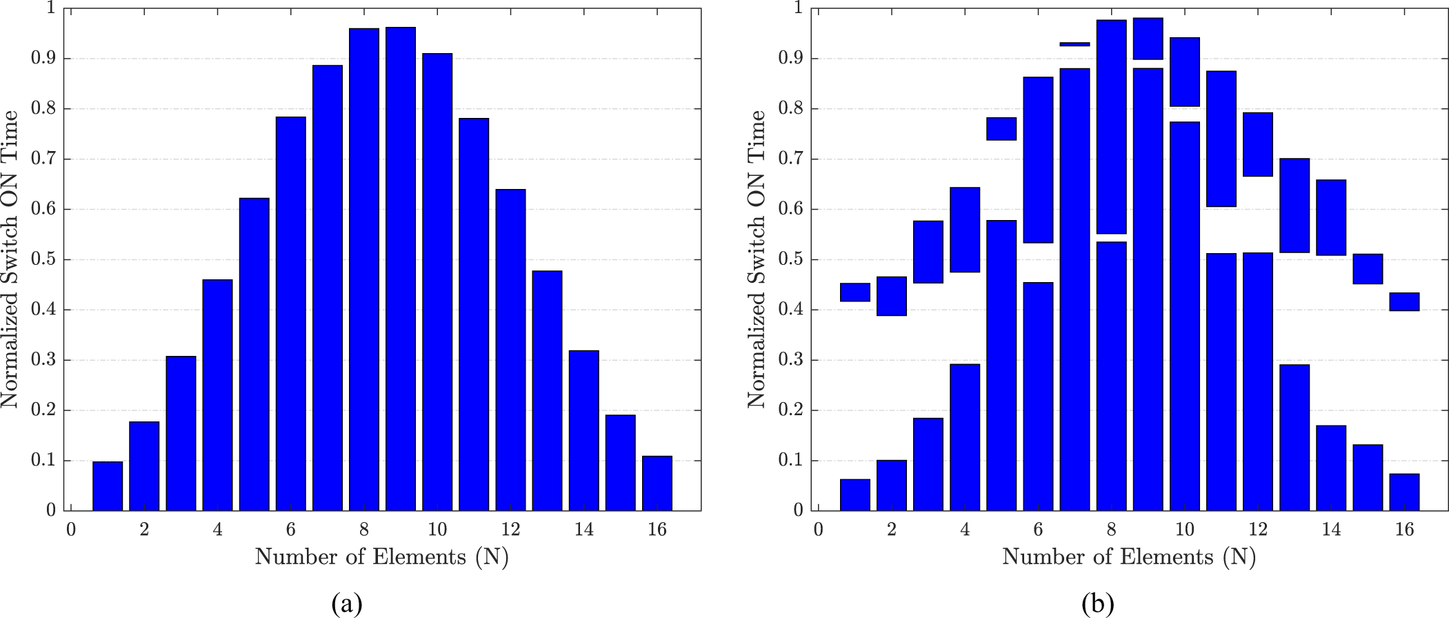
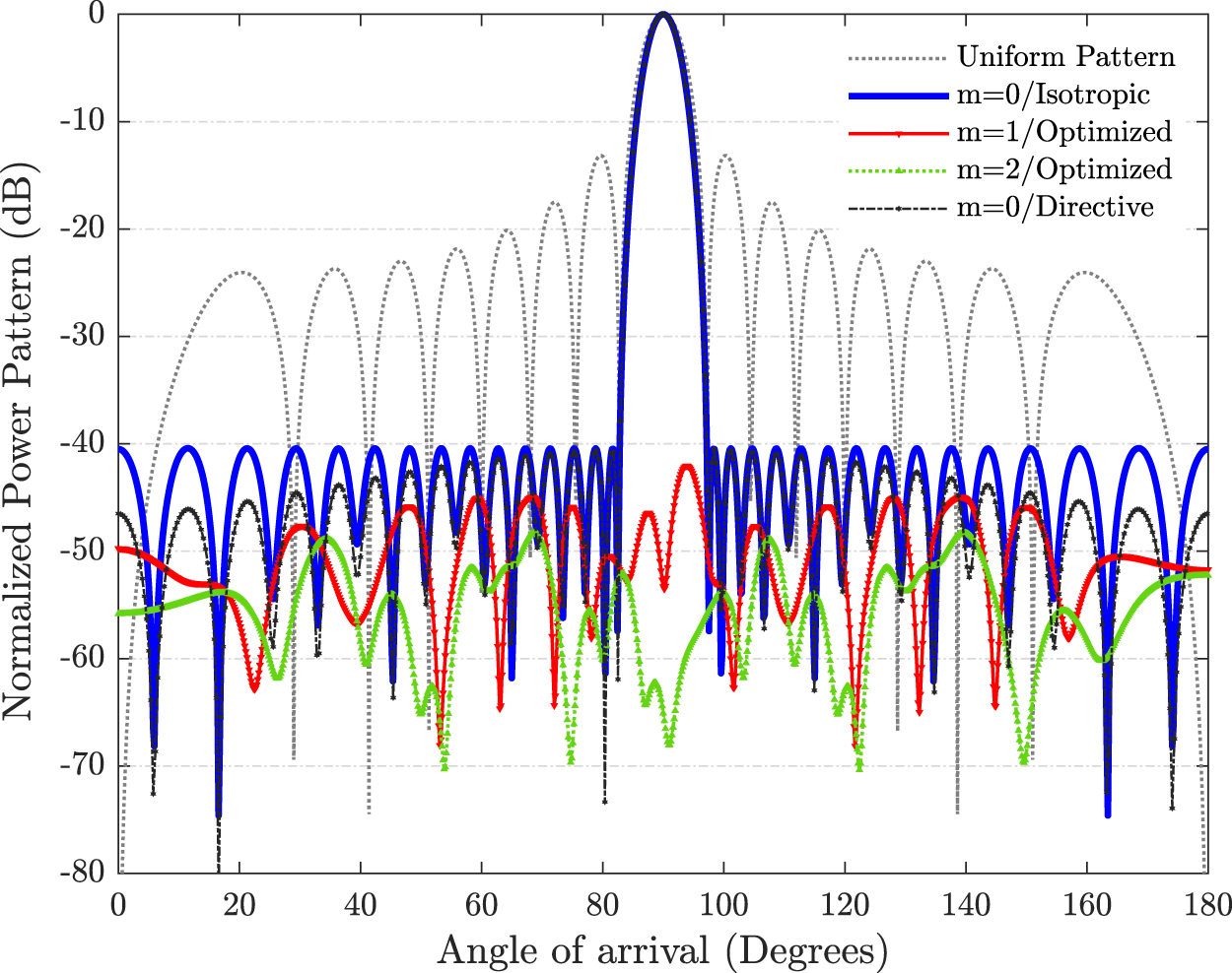
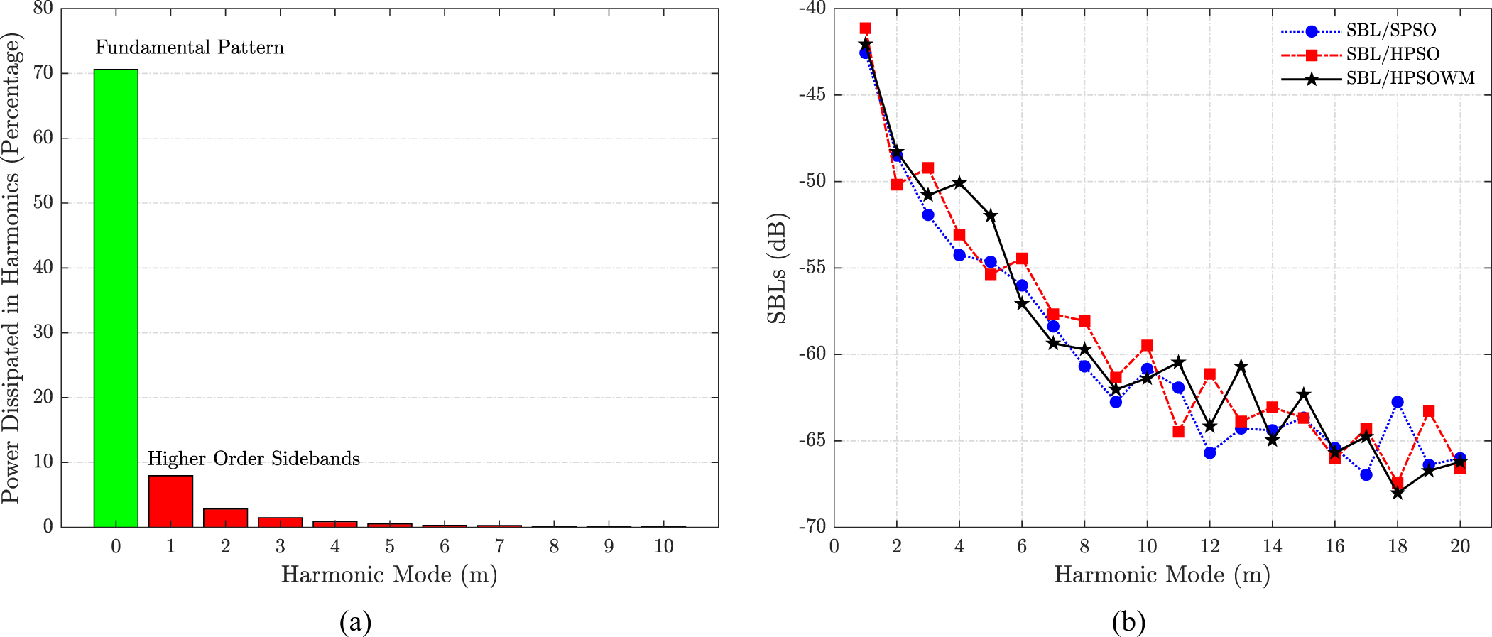
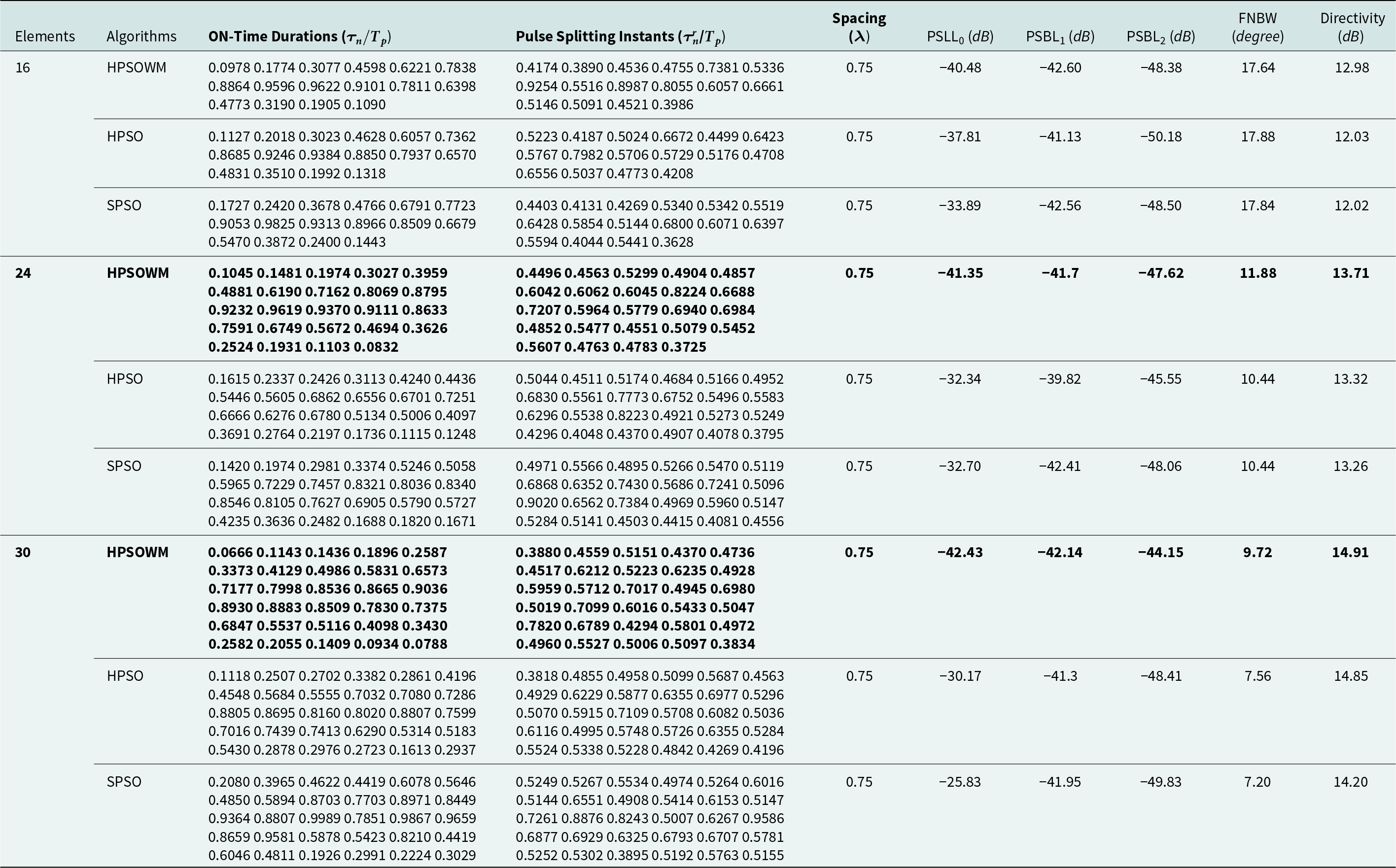
The 16-element beamforming 4D linear array is developed by aiming the objective of simultaneous SLL and SBLs reduction using pulse splitting. The ON-time and the pulse splitting instants of each array element are optimized, along with the uniform distance between each of them. The optimal outcomes are targeted by the proposed HPSOWM algorithm. The HPSOWM-based outcomes are also compared with HPSO and SPSO-based outcomes. To minimize the SBLs, the optimized ON-times of each antenna splits in two halves and shifted, so that the unwanted SRs can be outspread in a uniform way. The ON-times of the first pulse and the splitting instants of the second pulse are taken into account for optimization. Pulse splitting and shifting do not affect the central pattern, as central beam depends only upon the ON-time period. Thus, the central beam kept unchanged. The optimized beamforming switch schemes without and with pulse splitting derived by HPSOWM are presented in Fig. 4(a) and (b). The radiation pattern for point-to-point beamforming array is given in Fig. 5. Here, the uniform pattern, as well as the optimized main beam pattern ( ${f_0}$ at m = 0) with isotropic and directive elements are shown. The fixed inter-element spacing between each antenna is kept as 0.75λ. The radiation patterns obtained with HPSO and SPSO are also presented in Fig. 6(a) and (b), respectively. The proposed HPSOWM-based array is reported with a reduced PSLL of—40.48 dB compared to—13.15 dB PSLL of isophoric 4D array. HPSOWM-based pulse splitting approach also produces low SBLs, and the first two SBLs are reported as—42.6 dB and—48.38 dB. The FNBW and directivity reported for the proposed 4D array are 17.64º and 12.98 dB compared to 14.4º and 12.04 dB of isophoric array, respectively. The WM method is superior over the HPSO and SPSO methods as—37.81 dB and—33.89 dB PSLLs are obtained against—42.6 dB. The power at sideband is directly proportional to the nature of higher-order SBLs. The power generated at the main beam and first ten higher-order harmonics is shown in Fig. 7(a). In addition to that, the first twenty higher SBLs are also reported in Fig. 7(b) shows that the target objective of SLL and SBLs reduction are achieved simultaneously with the proposed 4D arrays. In the proposed beamforming array with HPSOWM, 70.61% power is utilized and 29.39% is wasted in higher-order harmonics compared to 70.01%, 29.99% and 68.72%, 31.28% obtained with HPSO and SPSO, respectively. The optimized numerical outcomes are shown in Table 1. The possible application of the proposed work is high-directive point-to-point communication system.
Optimal beamforming switch schemes (a) without and (b) with pulse splitting for 16-element array.

Optimal beamforming radiation patterns with reduced PSLL and sbls for 16-element array.

Beamforming radiation patterns 16-element array using (a) HPSO and (b) spso-based schemes.

(a) power dissipated in main beam and sidebands with HPSOWM, (b) optimized higher-order sbls.

Numerical results for the proposed beamforming 4D array with optimized time schemes

Beamforming with 24-element array
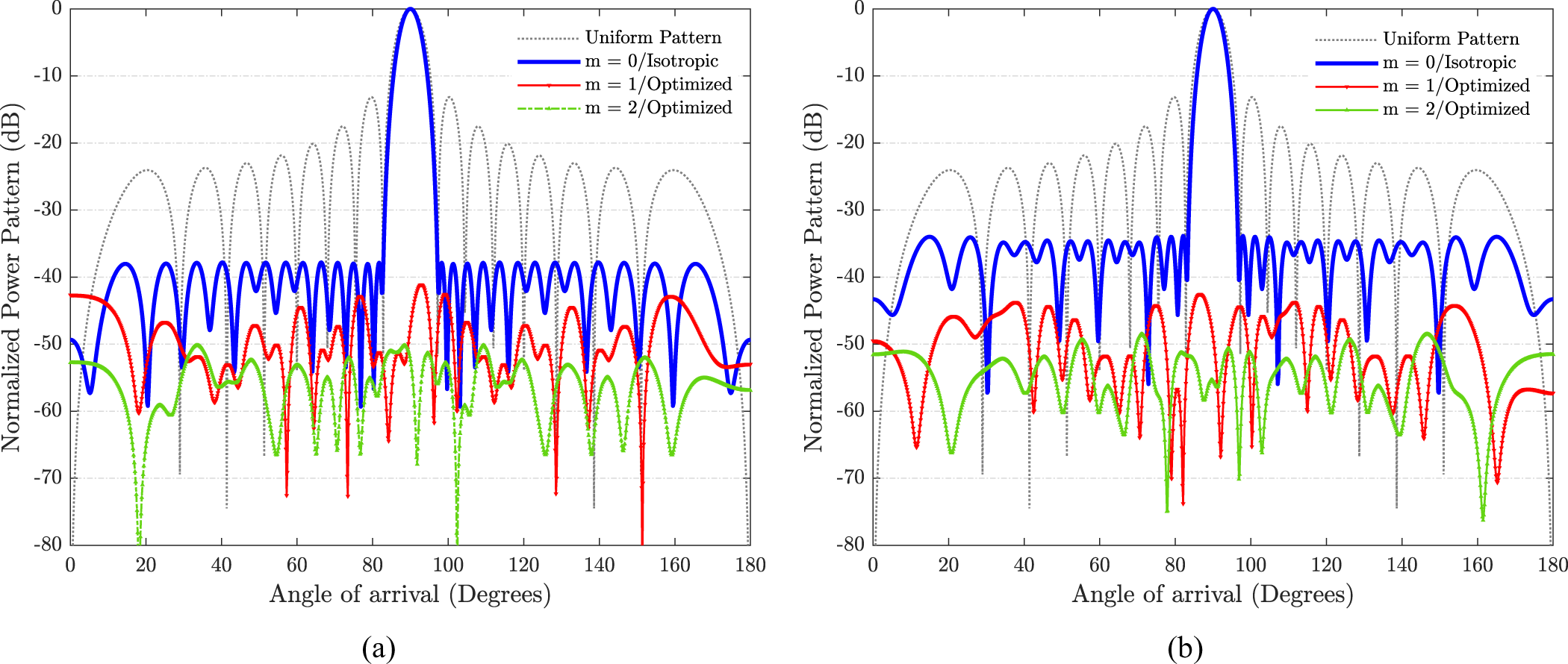
The 24-element beamforming 4D linear array is proposed here by aiming SLL and SBLs reduction simultaneously through pulse splitting. The ON-time and the pulse splitting instants of each array element are optimized. The optimal results are targeted by HPSOWM algorithm. The HPSOWM-based results are then compared with HPSO-based, SPSO-based and uniform 4D linear arrays. The optimized beamforming switch schemes without and with pulse splitting derived by HPSOWM are presented in Fig. 8(a) and (b). The radiation pattern for point-to-point beamforming array is given in Fig. 9. The fixed inter-element spacing of the array is kept as 0.75λ. The radiation patterns obtained with HPSO and SPSO are also shown in Fig. 10(a) and (b), respectively. The proposed HPSOWM-based array has a reduced PSLL of—41.35 dB compared to—13.21 dB of isophoric 4D array. HPSOWM-based pulse splitting approach also produces low SBLs, and the first two SBLs are reported as—41.7 dB and—47.62 dB. The FNBW and directivity reported for the proposed 4D array are 11.88º and 13.72 dB compared to 9.72º and 13.80 dB of the isophoric array, respectively. The WM method exhibits superiority over the HPSO and SPSO methods as—32.34 dB and—32.70 dB PSLLs are obtained against—41.35 dB. The power generated at the central beam and first ten higher-order harmonics is presented in Fig. 11(a). In addition to that, the first twenty higher SBLs are also reported in Fig. 11(b) shows that the objective of SLL and SBLs reduction are achieved simultaneously with the proposed 4D arrays. In the proposed beamforming array with HPSOWM, 70.16% power is utilized and 29.84% is wasted in higher-order harmonics compared to 63.38%, 36.62% and 52.43%, 47.57% obtained with HPSO and SPSO, respectively. The optimal numerical outcomes are shown in Table 1.
Optimal beamforming switch schemes (a) without and (b) with pulse splitting for 24-element array.

Optimal beamforming radiation patterns with reduced PSLL and sbls for 24-element array.

Beamforming radiation patterns 24-element array using (a) HPSO and (b) spso-based schemes.

(a) power dissipated in main beam and sidebands with HPSOWM, (b) optimized higher-order sbls.

Beamforming with 30-element array
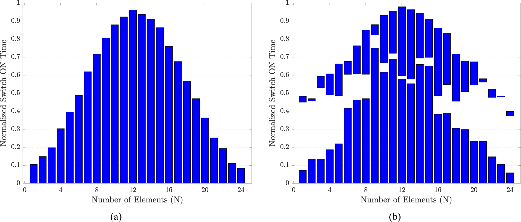
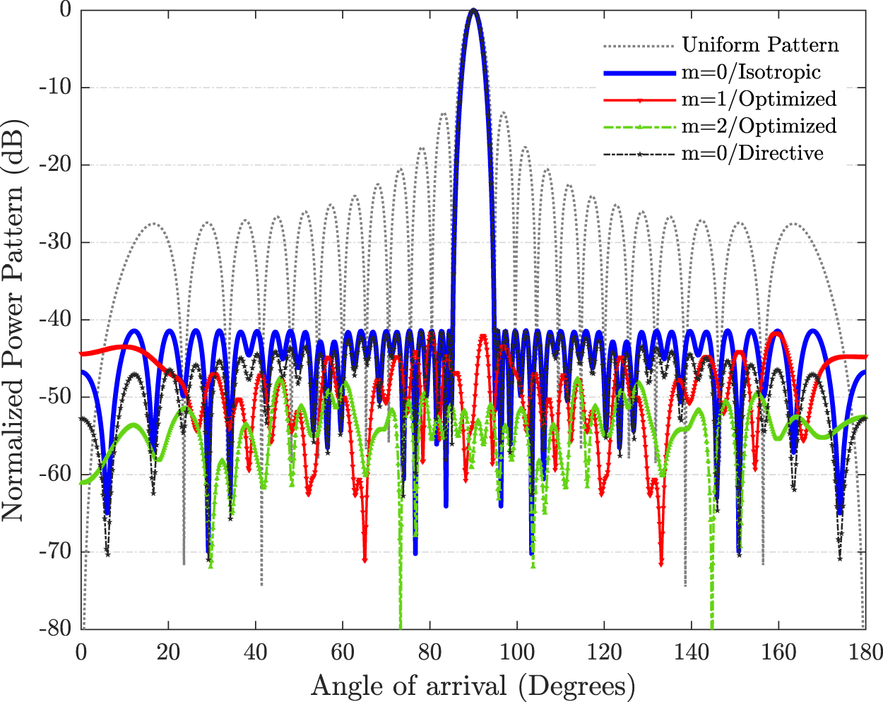
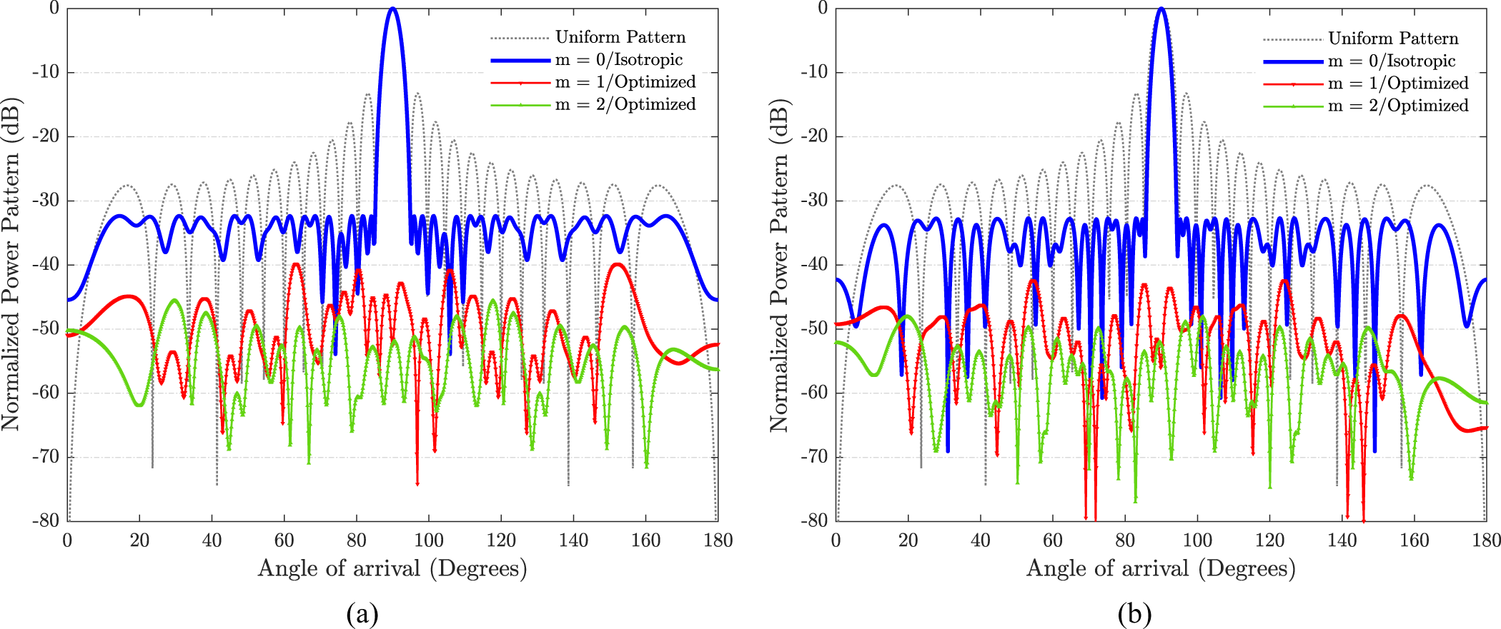
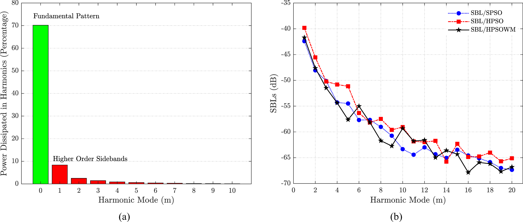
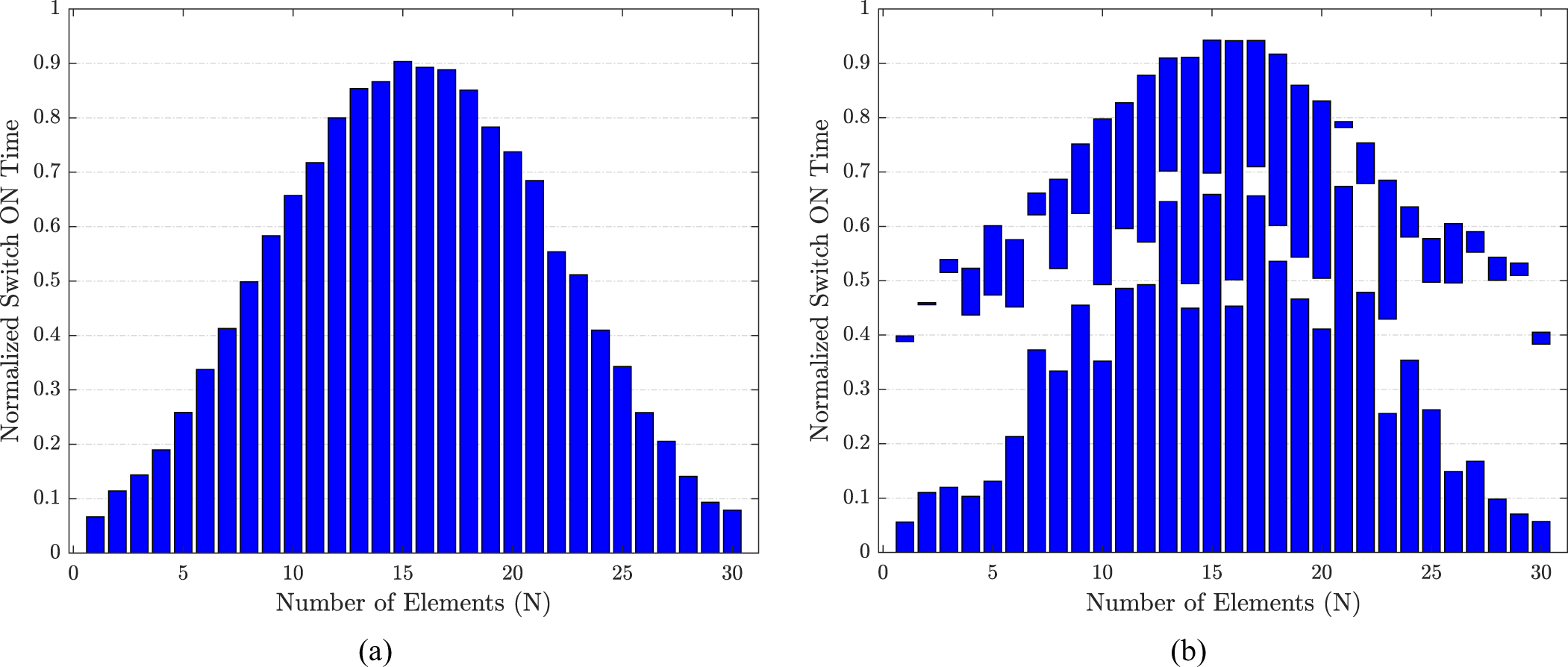
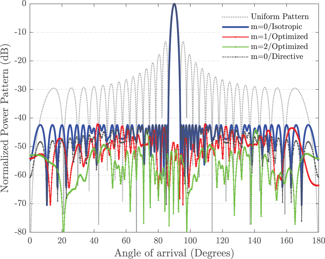
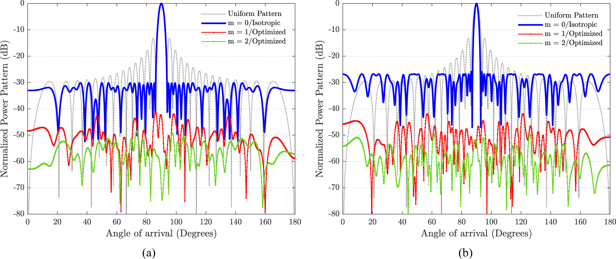
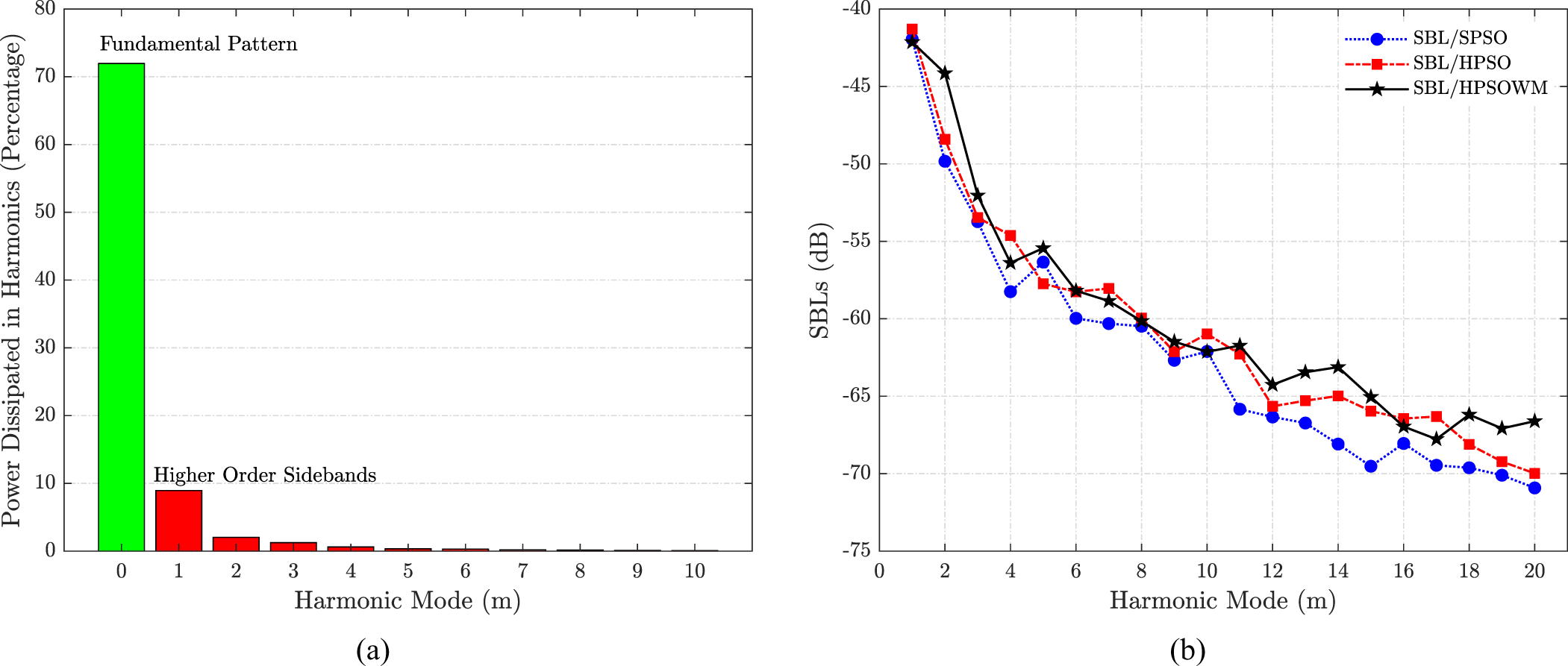
The 30-element beamforming 4D linear array is also proposed for the simultaneous SLL and SBLs reduction with pulse splitting. The optimal results are targeted by optimizing the ON-time and the pulse splitting instants of each antenna element using HPSOWM. The HPSOWM-based outcomes are compared with HPSO-based, SPSO-based and uniform 4D arrays. The optimized beamforming switch schemes without and with pulse splitting derived by HPSOWM are presented in Fig. 12(a) and (b). The radiation pattern for point-to-point beamforming array is given in Fig. 13. The fixed inter-element spacing of the array is kept as 0.75λ. The radiation patterns obtained with HPSO and SPSO are also shown in Fig. 14(a) and (b), respectively. The proposed HPSOWM-based array has a reduced PSLL of—42.43 dB compared to—13.24 dB of isophoric 4D array. HPSOWM-based pulse splitting approach also produces low SBLs and the first two SBLs are reported as—42.14 dB and—44.15 dB. The FNBW and directivity reported for the proposed 4D array are 9.72º and 14.91 dB compared to 7.56º and 14.77 dB of the isophoric array, respectively. The WM method exhibits superiority over the HPSO and SPSO methods as—30.17 dB and—25.83 dB PSLLs are obtained against—42.43 dB. The power generated at the central beam and first ten higher-order harmonics is presented in Fig. 15(a). In addition to that, the first twenty higher SBLs are also reported in Fig. 15(b) shows that the objective of SLL and SBLs reduction are achieved simultaneously with the proposed 4D arrays. In the proposed beamforming array with HPSOWM, 71.96% power is utilized and 28.04% is dissipated in higher-order harmonics compared to 63.54%, 36.46% and 61.96%, 28.04% obtained with HPSO and SPSO, respectively. The optimal numerical outcomes are shown in Table 1.
Optimal beamforming switch schemes (a) without and (b) with pulse splitting for 30-element array.

Optimal beamforming radiation patterns with reduced PSLL and sbls for 30-element array.

Beamforming radiation patterns 30-element array using (a) HPSO and (b) spso-based schemes.

(a) power dissipated in main beam and sidebands with HPSOWM, (b) optimized higher-order sbls.

Statistical test and comparison
To confirm the superiority of the WM method over HPSO and SPSO, two independents statistical  $t\_test$ analysis is performed for the optimization problem in hand. Assuming unequal variances or standard deviations (
 $\sigma _1^2 \ne \sigma _2^2$) for a population, the test statistics may be calculated as [Reference Scott, Walpole and Myers50]
 \begin{equation}{t_{test}} = \frac{{{{\bar \alpha }_{22}} - {{\bar \alpha }_{11}}}}{{\sqrt {\left( {\frac{{\sigma _1^2}}{{{n_A}}}} \right) + \left( {\frac{{\sigma _2^2}}{{{n_B}}}} \right)} }}\end{equation}
The degree of freedom (DoF) may be calculated as [Reference Scott, Walpole and Myers50]
 \begin{equation}\beta = \frac{{{{\left( {\frac{{\sigma _1^2}}{{{n_A}}} + \frac{{\sigma _2^2}}{{{n_B}}}} \right)}^2}}}{{\left\{ {\frac{{{{\left( {\frac{{\sigma _1^2}}{{{n_A}}}} \right)}^2}}}{{\left( {{n_A} - 1} \right)}} + \frac{{{{\left( {\frac{{\sigma _2^2}}{{{n_B}}}} \right)}^2}}}{{\left( {{n_B} - 1} \right)}}} \right\}}}\end{equation}
where,  ${\bar \alpha _{11}}$ and
 ${\bar \alpha _{22}}$ are the means;
 ${\sigma _1}$ and
 ${\sigma _2}$ are the standard deviations; and
 ${n_A}$,
 ${n_B}$ are the number of sample sizes considered for comparing the proposed algorithm with others. By considering
 ${n_A} = {n_B}$ for the 16-element 4D linear array, the
 $t\_test$ values obtained for different DoFs (
 $\beta $) comparing HPSOWM with HPSO and SPSO are presented in Table 2. The
 $t\_test$ values obtained are greater than the critical value [Reference Scott, Walpole and Myers50], and that ensures the existence of an indicative deviation in HPSOWM’s performance over HPSO and SPSO with 99.9% confidence.
Statistical  $t\_test$ comparisons for the proposed HPSOWM with HPSO and SPSO for 16-element array

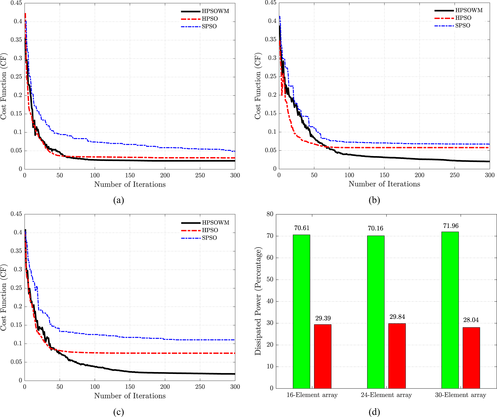
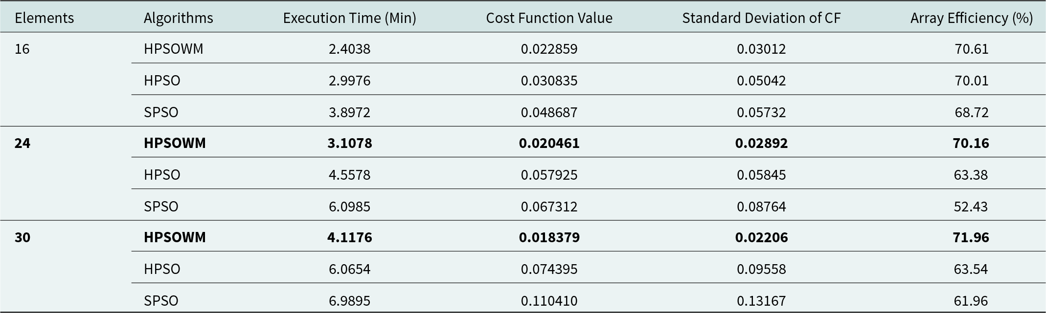
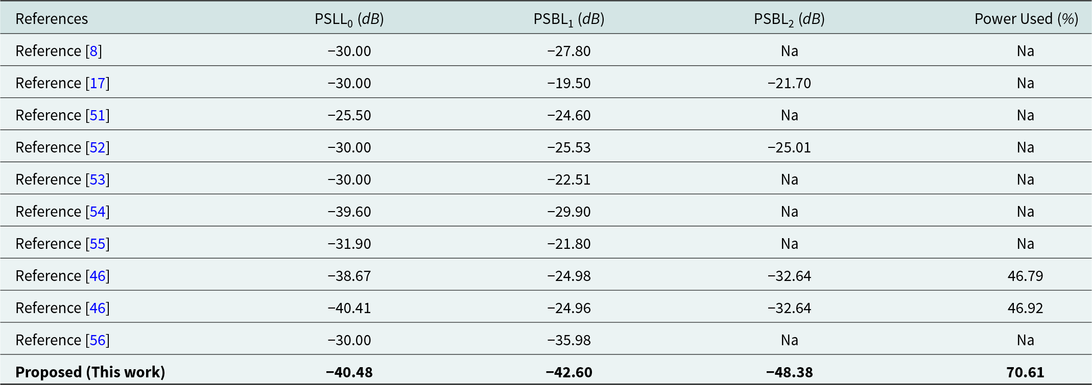
The convergence plots of each method for the proposed 16, 24, and 30-element 4D linear arrays are shown in Fig. 16(a), (b), and (c), respectively. A comparison of used and wasted power for the HPSOWM-based proposed arrays is reported in Fig. 16(d). Comparison of efficiencies of the proposed arrays with execution time and optimized cost function values are reported in Table 3. Apart from all these statistical comparisons, the proposed array is also compared with other state of the art results, and presented in Table 4. The WM-based results show better performance in terms of array radiation properties compared to all the already reported works. Hence, a conclusion can be drawn that the proposed method is very well-suited for high-directive, secure point-to-point communication systems.
Convergence plots for (a) 16-element, (b) 24-element, (c), 30-element 4D array, and (d) comparison of used and unused power for hpsowm-based proposed 4D arrays.

Comparison of efficiency of proposed array with execution time and optimized cost function values

Comparison of the proposed hpsowm-based outcomes with other works for 16-element array

Conclusion
The adaptive radiation characteristics of fourth-dimensional (4D) linear antenna arrays have been explored in this article for beamforming applications. The point-to-point wireless communication system requires efficient, well-controlled, and optimized radiations patterns in specific directions. Contributions: The proposed array has achieved the target of ultra-low sidelobes beneficial for highly directive wireless transmission and reception. Simultaneously, the sideband levels (SBLs) have been reduced to minimize power distortion. The optimality of the array has further enhanced by introducing a hybrid particle swarm optimizer with wavelet-based mutation approach. The problems in hand are formulated in a single-objective cost function (CF) to optimize the beamforming network (BFN) consists of optimal ON-time duration and ON-time instances of the splitting pulses. The optimal switching sequences have been derived for three sets of linear 4D arrays by considering the target sidelobe below—40 dB. The inherent limitation of time-modulation, i.e., the formation of sidelobes at the multiple of harmonic frequencies have also been taken care of by proposing efficient pulse splitting techniques for all the arrays. The detailed comparison of the proposed array with simple PSO and hybrid PSO-based 4D arrays have also been reported which shows the effectiveness of the newly adopted mutation technique inspired by Morlet wavelets. Benefits: The targets have been attained with a reduction in SLL and SBLs below—40.48,—42.6 and—48.38 dB. The optimally splitting pulses-based single BFN also eliminates the implementational complexities. The power calculation has also shown that the arrays utilized more than 70% power in the main beam which indicates good beamforming performances for all three sets of arrays. Furthermore, the investigation of other reported works in this domain have also been carried over to compare the proposed array antenna. The comparison shown for 16-element array establishes the superiority of the proposed research as more than—40 dB SLL and SBLs compared to around—35 dB SLL and SBLs of the best-reported literature. Finally, it can be concluded that all the three sets of arrays with reduced sidelobes and sidebands are applicable for directive wireless signal transmission or reception, and can further be explored in near future for more advanced applications.
Data Availability Statement
No new data were created or analyzed during this study. Data sharing is not applicable to this article.
Competing interests
The authors declare that they have no known competing financial interests or personal relationships that could have appeared to influence the work reported in this paper.