1 Introduction
Many geophysical and astrophysical objects can be looked upon as rotating spherical shells. A prime example would be the fluid outer core of the Earth harbouring the geodynamo. Other examples are dynamo regions of other terrestrial and gas planets, planetary atmospheres as well as convection zones of stars. The dynamics in these shells is commonly thought to be driven by convection, with an important role played by the Coriolis force. However, differential rotation could also have a significant impact and is discussed as an alternative driving mechanism in stellar radiative zones (Spruit Reference Spruit2002; Potter, Chitre & Tout Reference Potter, Chitre and Tout2012). Here we study the role of differential rotation in a rotating system with a simple spherical Couette set-up.
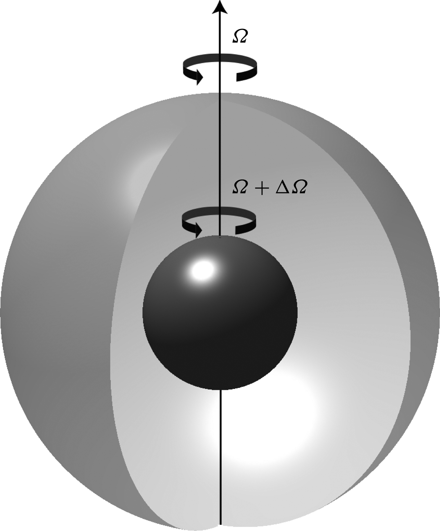
The spherical Couette system consists of a viscous fluid filling the gap between two concentric spheres, as shown in figure 1. The flow is driven by the differential rotation of the two boundaries. This relatively simple system demonstrates multiple fluid dynamic phenomena, including free shear layers, transition to turbulence, Coriolis-restored oscillations and a lot more. Besides having potential applications to astrophysical objects, it is also an interesting fundamental fluid dynamical system.
The spherical Couette system. The outer boundary rotates at a rate
 $\unicode[STIX]{x1D6FA}$
while the inner one rotates at a rate
 $\unicode[STIX]{x1D6FA}+\unicode[STIX]{x0394}\unicode[STIX]{x1D6FA}$
.

Though in principle very similar to the better known cylindrical Couette–Taylor system, for the wide-gap spherical Couette set-up studied here, even the primary instabilities are already different (Egbers & Rath Reference Egbers and Rath1995). It has been studied in the past analytically (e.g. Proudman Reference Proudman1956; Bratukhin Reference Bratukhin1961; Stewartson Reference Stewartson1966; Munson & Joseph Reference Munson and Joseph1971a ,Reference Munson and Joseph b ), experimentally (e.g. Sorokin, Khlebutin & Shaidurov Reference Sorokin, Khlebutin and Shaidurov1966; Munson & Menguturk Reference Munson and Menguturk1975; Egbers & Rath Reference Egbers and Rath1995; Kelley et al. Reference Kelley, Triana, Zimmerman, Tilgner and Lathrop2007, Reference Kelley, Triana, Zimmerman and Lathrop2010; Zimmerman Reference Zimmerman2010; Triana Reference Triana2011; Schmitt et al. Reference Schmitt, Cardin, Rizza and Nataf2013; Hoff, Harlander & Triana Reference Hoff, Harlander and Triana2016b ) as well as numerically (e.g. Hollerbach Reference Hollerbach2003; Hollerbach et al. Reference Hollerbach, Futterer, More and Egbers2004; Matsui et al. Reference Matsui, Adams, Kelley, Triana, Zimmerman, Buffett and Lathrop2011; Wicht Reference Wicht2014). These studies have shown that the spherical Couette system is host to a lot of different types of instabilities depending on the parameter space explored.
We focus here on the more geo- and astrophysically relevant regime of rapid outer boundary rotation. In this regime, the cylinder tangent to the inner sphere at the equator, also known as the tangent cylinder (TC) forms an important boundary. The fluid in the region outside the TC is in solid-body rotation with the outer boundary, while that in the region inside the TC rotates at approximately half the differential rotation rate. A complex free Stewartson shear layer (Proudman Reference Proudman1956; Stewartson Reference Stewartson1966) develops on the boundary between these two regions. The first instabilities in the system in this regime are nearly geostrophic Stewartson layer instabilities (SI), with the critical wavenumber and differential rotation being dependent on whether the inner sphere rotates faster (positive differential rotation) or slower (negative differential rotation) with respect to the outer one (Hollerbach Reference Hollerbach2003). For example, in the former case, wavenumbers are typically large; while in the latter case, the first instability has wavenumber one for not too fast outer boundary rotations (e.g. Hollerbach Reference Hollerbach2003; Wicht Reference Wicht2014).
One of the most interesting instabilities seen in this system are inertial modes which are oscillations in a rotating fluid restored by the Coriolis force. These modes have been observed only for negative differential rotation in the spherical Couette experiments (Kelley et al. Reference Kelley, Triana, Zimmerman, Tilgner and Lathrop2007, Reference Kelley, Triana, Zimmerman and Lathrop2010; Kelley Reference Kelley2009; Triana Reference Triana2011; Rieutord et al. Reference Rieutord, Triana, Zimmerman and Lathrop2012; Hoff et al. Reference Hoff, Harlander and Triana2016b ) as well as in the direct numerical simulations (Matsui et al. Reference Matsui, Adams, Kelley, Triana, Zimmerman, Buffett and Lathrop2011; Wicht Reference Wicht2014). Inertial modes are expected to be observed in systems with rapid rotation and low viscosity, as observed in a rapidly rotating B3 star (Pápics et al. Reference Pápics, Briquet, Baglin, Poretti, Aerts, Degroote, Tkachenko, Morel, Zima and Niemczura2012) and in a hot Be star (Neiner et al. Reference Neiner, Floquet, Samadi, Espinosa Lara, Frémat, Mathis, Leroy, de Batz, Rainer and Poretti2012) in the form of gravito-inertial modes. The linear eigenvalue problem of inertial modes in a spherical shell has been extensively studied (e.g. Rieutord Reference Rieutord1991; Rieutord & Valdettaro Reference Rieutord and Valdettaro1997; Tilgner Reference Tilgner1999; Rieutord, Georgeot & Valdettaro Reference Rieutord, Georgeot and Valdettaro2001; Rieutord et al. Reference Rieutord, Triana, Zimmerman and Lathrop2012; Baruteau & Rieutord Reference Baruteau and Rieutord2013).
However, despite all the above studies on both the spherical Couette system as well as the linear inertial mode problem, several open questions remain. First and foremost, it remains unclear why specific modes are excited at certain critical differential rotation rates in the absence of periodic exciting mechanisms like libration, precession or tidal forcing (Le Bars, Cébron & Le Gal Reference Le Bars, Cébron and Le Gal2015). Secondly, some of these modes show departures from the eigenmodes of a spherical shell or a full sphere in terms of drift frequency and structure. Thirdly, the most dominant modes observed are ‘fast’ (explained in § 2.2) and antisymmetric with respect to the equator. This is a surprise because the driving mechanism of the whole system is symmetric. Moreover, the fast outer boundary rotation generally enforces geostrophic solutions and these inertial modes are clearly an exception. Lastly, these modes are more prominent for ‘negative’ differential rotation.
Past studies have tried to explain the onset and selection of modes using the theory of over-reflection (Kelley et al. Reference Kelley, Triana, Zimmerman and Lathrop2010) or being excited due to a critical layer at the TC (Rieutord et al. Reference Rieutord, Triana, Zimmerman and Lathrop2012). The theory of over-reflection by Kelley et al. (Reference Kelley, Triana, Zimmerman and Lathrop2010) is based on the theory applied to sound waves, and thus requires a more detailed investigation of its applicability to inertial waves. In addition, it does not fully explain all the mode selections observed in the experiment. The critical layer is an alternative theory proposed by Rieutord et al. (Reference Rieutord, Triana, Zimmerman and Lathrop2012), and requires further investigation to clarify its applicability.
In the present study, we first compare experimental results from spherical Couette experiments at BTU Cottbus-Senftenberg (Hoff et al. Reference Hoff, Harlander, Egbers, Triana, Egbers, Ruck, Leder and Dopheide2016a ,Reference Hoff, Harlander and Triana b ), henceforth referred to as ‘BTU C-S’, with results from numerical simulations of two different codes. Having established the applicability of the numerical schemes, we then proceed to perform numerical experiments to provide further insight into the system and answer some of the open questions mentioned above.
The rest of the paper is arranged as follows. Section 2 gives a short theoretical background on the spherical Couette system and inertial modes. Section 3 provides a brief overview of experimental methods and the main results. Sections 4 and 5 present the numerical methods and simulation results while comparing them with those from the experiment. Section 6 explores the effect of the background flow on an inertial mode. Section 7 discusses triadic resonances observed in the system. Section 8 discusses numerical experiments performed to understand the onset of inertial modes. Lastly, the paper ends with a summary of the main results and their conclusions.
2 Theoretical background
2.1 The spherical Couette system
The spherical Couette system is illustrated in figure 1. It consists of concentric inner and outer spheres with radii
 $r_{i}$
and
 $r_{o}$
, respectively, with a viscous fluid in between. We use a frame of reference rotating with the outer boundary. The time evolution of the flow in this system can be expressed in terms of the Navier–Stokes and continuity equations,
 $$\begin{eqnarray}\displaystyle & \displaystyle \frac{\unicode[STIX]{x2202}\boldsymbol{u}}{\unicode[STIX]{x2202}t}=-\frac{1}{\unicode[STIX]{x1D70C}}\unicode[STIX]{x1D735}p-\boldsymbol{u}\boldsymbol{\cdot }\unicode[STIX]{x1D735}\boldsymbol{u}-2\unicode[STIX]{x1D6FA}_{o}\hat{\boldsymbol{z}}\times \boldsymbol{u}+\unicode[STIX]{x1D708}\unicode[STIX]{x1D6FB}^{2}\boldsymbol{u}, & \displaystyle\end{eqnarray}$$
 $$\begin{eqnarray}\displaystyle & \displaystyle \unicode[STIX]{x1D735}\boldsymbol{\cdot }\boldsymbol{u}=0. & \displaystyle\end{eqnarray}$$
Here,
 $\boldsymbol{u}$
,
 $\unicode[STIX]{x1D70C}$
and
 $\unicode[STIX]{x1D6FA}_{o}$
represent the velocity of the fluid, the density of the fluid and rotation rate of the outer boundary, respectively. The unit vector in the direction of rotation is denoted by
 $\hat{\boldsymbol{z}}$
, while
 $p$
denotes an effective pressure, which includes the contribution of gravity and centrifugal forces.
Using the shell width,
 $L=r_{o}-r_{i}$
, as a length scale and the viscous diffusion time,
 $L^{2}/\unicode[STIX]{x1D708}$
, as a time scale, we define the Ekman number as
 $$\begin{eqnarray}\displaystyle & \displaystyle E=\unicode[STIX]{x1D708}/\unicode[STIX]{x1D6FA}_{o}L^{2}=1/\unicode[STIX]{x1D6FA}, & \displaystyle\end{eqnarray}$$
where
 $\unicode[STIX]{x1D6FA}_{o}$
and
 $\unicode[STIX]{x1D6FA}$
are the dimensional and non-dimensional outer boundary rotation rates respectively, and
 $\unicode[STIX]{x1D708}$
is the kinematic viscosity.
The differential rotation is quantified using
 $$\begin{eqnarray}\displaystyle & \displaystyle \unicode[STIX]{x0394}\unicode[STIX]{x1D6FA}/\unicode[STIX]{x1D6FA}=(\unicode[STIX]{x1D6FA}_{i}-\unicode[STIX]{x1D6FA}_{o})/\unicode[STIX]{x1D6FA}_{o}, & \displaystyle\end{eqnarray}$$
where
 $\unicode[STIX]{x1D6FA}_{i}$
is the dimensional inner boundary rotation rate and
 $\unicode[STIX]{x0394}\unicode[STIX]{x1D6FA}$
is the non-dimensional differential rotation rate of the inner boundary with respect to the outer. Thus,
 $\unicode[STIX]{x0394}\unicode[STIX]{x1D6FA}<0$
would imply that the inner sphere rotates slower or in the opposite direction with respect to the outer sphere, while
 $\unicode[STIX]{x0394}\unicode[STIX]{x1D6FA}>0$
would mean that the inner sphere rotates faster than the outer sphere in the same direction.
The equations are completed with the impenetrable and no-slip boundary conditions:
 $$\begin{eqnarray}\displaystyle \left.\begin{array}{@{}c@{}}\displaystyle \boldsymbol{u}(r_{o})=\mathbf{0},\\ \displaystyle \boldsymbol{u}(r_{i})=(u_{r},u_{\unicode[STIX]{x1D703}},u_{\unicode[STIX]{x1D719}})=(0,0,(\unicode[STIX]{x1D6FA}_{i}-\unicode[STIX]{x1D6FA}_{o})r_{i}).\end{array}\right\} & & \displaystyle\end{eqnarray}$$
2.2 Inertial modes
Inertial modes are eigenmodes of the linear inviscid Navier–Stokes equation,
 $$\begin{eqnarray}\displaystyle & \displaystyle \frac{\unicode[STIX]{x2202}\boldsymbol{u}}{\unicode[STIX]{x2202}t}=-\displaystyle \frac{1}{\unicode[STIX]{x1D70C}}\unicode[STIX]{x1D735}p-2\unicode[STIX]{x1D6FA}\hat{\boldsymbol{z}}\times \boldsymbol{u}, & \displaystyle\end{eqnarray}$$
in a bounded container subject to the impenetrable boundary condition
 $\boldsymbol{u}\boldsymbol{\cdot }\hat{\boldsymbol{n}}=0$
, where
 $\unicode[STIX]{x1D6FA}$
represents the rotation rate of the container, and
 $\hat{\boldsymbol{n}}$
is the unit vector normal to the surface of the container.
Taking the curl of (2.6) twice and performing some algebra yields
 $$\begin{eqnarray}\displaystyle & \displaystyle \frac{\unicode[STIX]{x2202}^{2}\unicode[STIX]{x1D6FB}^{2}\boldsymbol{u}}{\unicode[STIX]{x2202}t^{2}}+4\unicode[STIX]{x1D6FA}^{2}\frac{\unicode[STIX]{x2202}^{2}\boldsymbol{u}}{\unicode[STIX]{x2202}z^{2}}=0, & \displaystyle\end{eqnarray}$$
where
 $z$
denotes the coordinate along the axis of rotation. This equation supports wave-like modes
 $$\begin{eqnarray}\displaystyle & \displaystyle \boldsymbol{u}(r,\unicode[STIX]{x1D703},\unicode[STIX]{x1D719})=\boldsymbol{Q}(r,\unicode[STIX]{x1D703})\text{e}^{\text{i}(m\unicode[STIX]{x1D719}-\unicode[STIX]{x1D714}t)}=\boldsymbol{Q}(r,\unicode[STIX]{x1D703})\text{e}^{\text{i}m(\unicode[STIX]{x1D719}-c_{d}t)}, & \displaystyle\end{eqnarray}$$
where we have used spherical coordinates. Here,
 $m$
represents the azimuthal wavenumber,
 $\unicode[STIX]{x1D714}$
is the drift frequency and
 $c_{d}=\unicode[STIX]{x1D714}/m$
is the drift speed. The eigenvalues
 $\unicode[STIX]{x1D714}$
are real and
 $|\unicode[STIX]{x1D714}|\leqslant 2\unicode[STIX]{x1D6FA}$
(Greenspan Reference Greenspan1968). We use the convention of denoting retrograde (prograde) modes with positive (negative) frequencies. The inertial mode problem is mathematically ill-posed in general (Stewartson & Rickard Reference Stewartson and Rickard1969), but smooth solutions can be obtained for certain containers, like cylinders and spheres. These modes are also known to exist in slightly modified form in viscous systems when rotational effects dominate viscous effects (e.g. Kelley et al.
Reference Kelley, Triana, Zimmerman, Tilgner and Lathrop2007; Triana Reference Triana2011; Wicht Reference Wicht2014).
In the following, we shall compare the observed inertial modes with those of a sphere whose modes have been studied for a long time (Bryan Reference Bryan1889) and for which explicit analytical solutions have been found by Zhang et al. (Reference Zhang, Earnshaw, Liao and Busse2001). For a spherical shell, in the absence of analytical solutions (Stewartson & Rickard Reference Stewartson and Rickard1969), one turns towards numerical eigenmode computations (e.g. Rieutord Reference Rieutord1991). For the present study we shall be using the eigenmodes computed using the code SINGE (Vidal & Schaeffer Reference Vidal and Schaeffer2015) for comparisons.
The inertial modes of a sphere can be characterised using three indices
 $(l,m,n)$
(indices
 $(n,k,m)$
of Greenspan (Reference Greenspan1968)), where
 $l$
and
 $m$
have the same meaning as the degree and order, respectively, of a spherical harmonic, and the third index denotes the
 $n$
th eigenmode corresponding to the combination
 $(l,m)$
. However, in our present study we identify a mode by using the indices
 $(l,m)$
and its frequency
 $\unicode[STIX]{x1D714}/\unicode[STIX]{x1D6FA}$
. The indices refer to the spherical harmonic structure at the surface,
 $r=r_{o}$
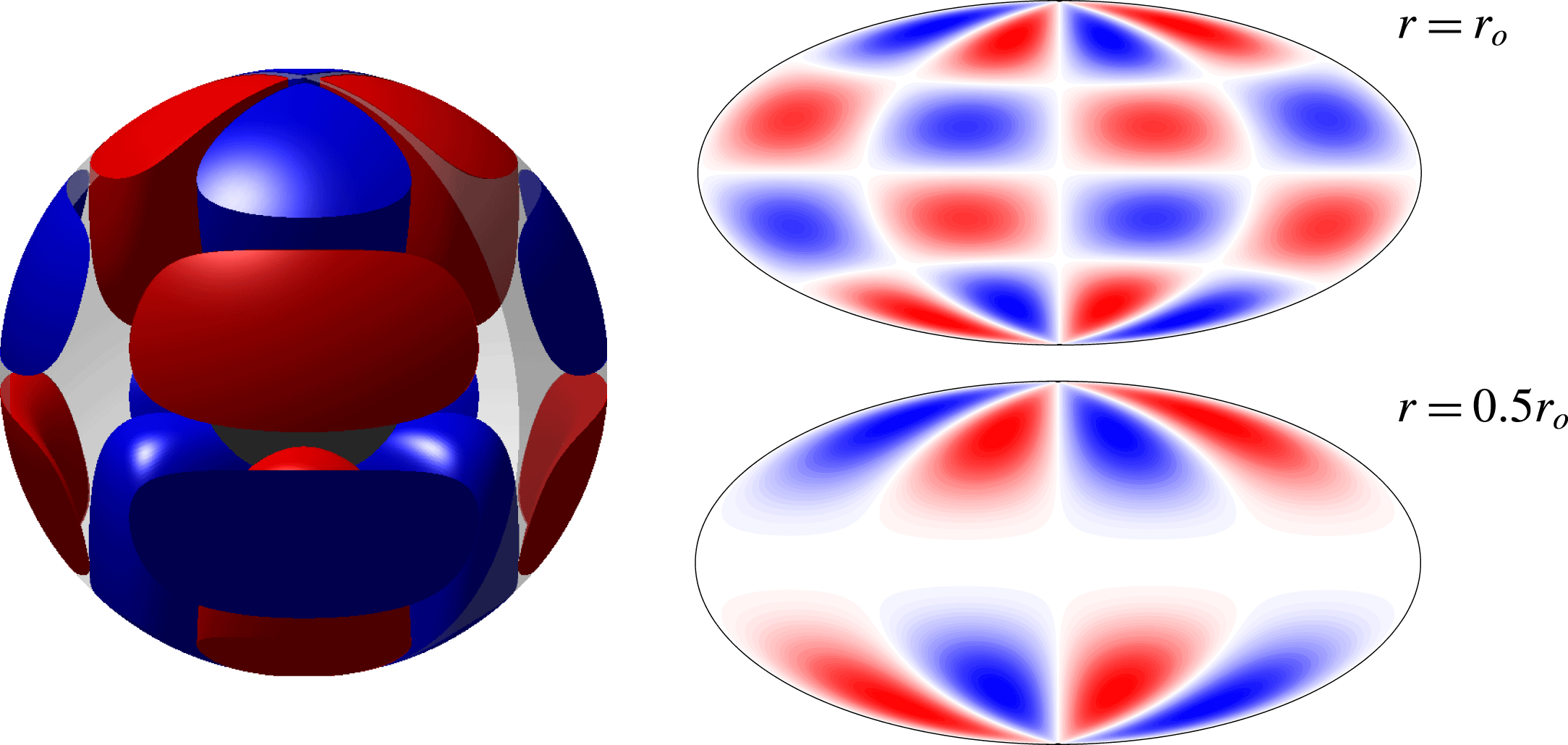
. At depth, the structure and thus the spherical harmonic contribution changes, as is illustrated in figure 2 for the mode
 $(5,2,0.467)$
.
The
 $(5,2,0.467)$
mode of a full sphere. The mode has the structure of the spherical harmonic
 $Y_{52}$
at the surface while that of
 $Y_{32}$
at mid-depth. Colours represent cylindrical radial velocity
 $u_{s}$
, with red (blue) being away from (towards) the rotation axis. The two-dimensional maps are hammer projections of the same quantity.

Inertial modes in a full sphere can be equatorially symmetric or antisymmetric. The equatorially symmetric modes that we find in simulations are the slow inertial modes described by Zhang et al. (Reference Zhang, Earnshaw, Liao and Busse2001) which are ‘nearly geostrophic’. This implies that they satisfy the Taylor–Proudman constraint to a large extent, i.e. the pressure gradient and Coriolis forces roughly balance each other,
 $$\begin{eqnarray}\displaystyle & \displaystyle -\text{i}\unicode[STIX]{x1D714}\boldsymbol{u}=-\unicode[STIX]{x1D735}p/\unicode[STIX]{x1D70C}-2\unicode[STIX]{x1D6FA}\hat{\boldsymbol{z}}\times \boldsymbol{u}\approx 0. & \displaystyle\end{eqnarray}$$
In such a scenario, the frequencies of these modes,
 $\unicode[STIX]{x1D714}$
, are ‘small’ in magnitude as compared to the boundary rotation
 $\unicode[STIX]{x1D6FA}$
and can thus change by a large fraction even for a small mismatch between pressure gradient and the Coriolis force. This is in contrast to the equatorially antisymmetric modes for which no such slow modes are found and which completely defy the Taylor–Proudman constraint and have larger magnitudes of frequencies as compared to the slow, nearly geostrophic, modes. Owing to this clear distinction between the frequencies of these two classes of modes, the equatorially antisymmetric modes were referred to as ‘fast inertial modes’ by Wicht (Reference Wicht2014). Thus, while the fast modes are easily identified by their frequencies, the same cannot be said of the slow columnar modes whose frequencies are susceptible to the slightest of changes in the force balance.
3 Experiments at BTU Cottbus-Senftenberg
The set-up for the spherical Couette experiments at BTU C-S, Germany, consists of two concentric rotating spheres with radii
 $r_{i}=40~\text{mm}$
and
 $r_{o}=120~\text{mm}$
, which translates to an aspect ratio of
 $r_{i}/r_{o}=1/3$
. The fluid in the gap is a silicone oil of viscosity
 $\unicode[STIX]{x1D708}=(0.65\pm 0.07)~\text{mm}^{2}~\text{s}^{-1}$
. Two ramps in differential rotation were performed at Ekman numbers of
 $E=3.04\times 10^{-5}$
and
 $1.52\times 10^{-5}$
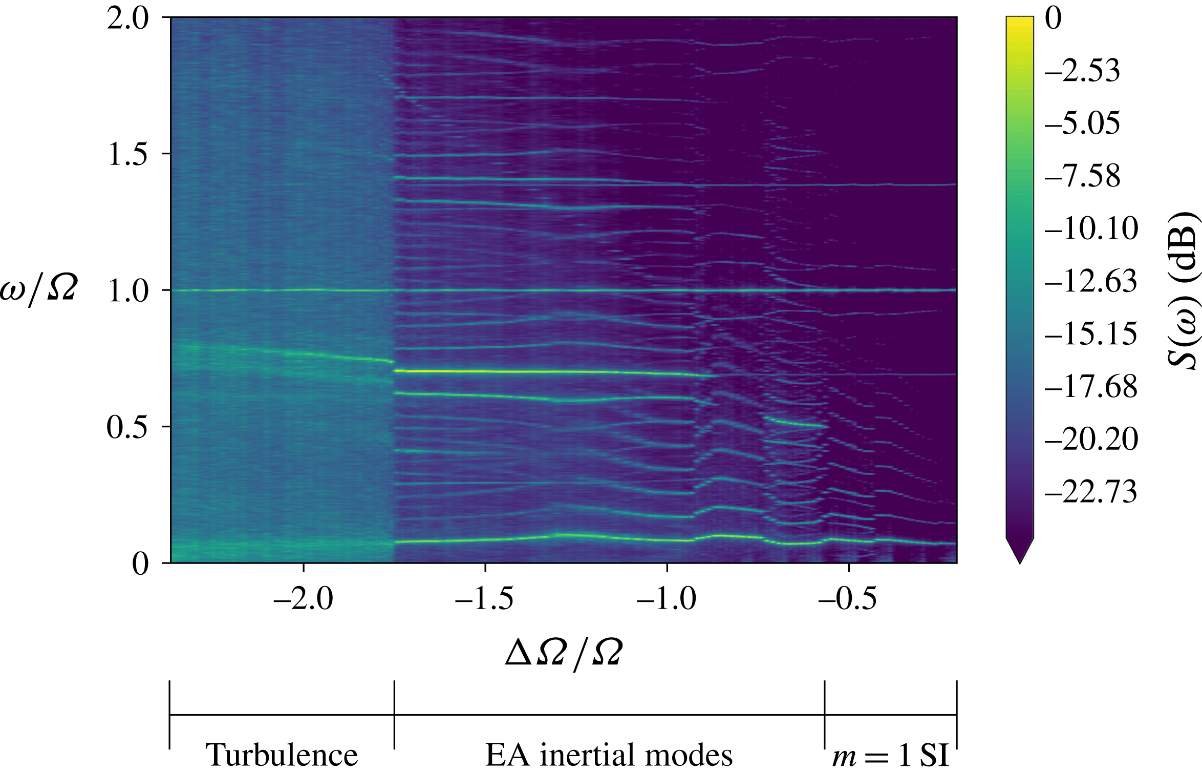
. The flow is visualised in the meridional plane using Kalliroscope particles and a vertical laser sheet. In the horizontal plane, the flow was characterised using particle image velocimetry (PIV), using hollow spherical glass spheres as tracers and a horizontal laser sheet. A Fourier analysis of the horizontal flow components gave spectrograms which were used to identify hydrodynamic regimes (figure 3 shows an example). Further details of the experimental set-up and analysis techniques can be found in Koch et al. (Reference Koch, Harlander, Egbers and Hollerbach2013) and Hoff et al. (Reference Hoff, Harlander, Egbers, Triana, Egbers, Ruck, Leder and Dopheide2016a
,Reference Hoff, Harlander and Triana
b
).
Spectrogram from PIV measurements of azimuthal velocity from experiments at BTU C-S,
 $u_{\unicode[STIX]{x1D719}}$
at
 $E=1.52\times 10^{-5}$
. One can see three distinct hydrodynamic regimes described by Hoff et al. (Reference Hoff, Harlander and Triana2016b
). Abbreviations: SI = Stewartson layer instability, EA = equatorially antisymmetric.

Hoff et al. (Reference Hoff, Harlander and Triana2016b
) describe the following three distinct hydrodynamic regimes encountered while increasing the magnitude of differential rotation (
 $|\unicode[STIX]{x0394}\unicode[STIX]{x1D6FA}/\unicode[STIX]{x1D6FA}|$
) from small to large values for a fixed outer boundary rotation rate (
 $\unicode[STIX]{x1D6FA}=1/E$
).
(i) Fundamental instability: At a critical differential rotation rate,
 $(\unicode[STIX]{x0394}\unicode[STIX]{x1D6FA}/\unicode[STIX]{x1D6FA})_{c}$
, the flow changes its state from a purely axisymmetric configuration to a non-axisymmetric one, with a well-defined azimuthal symmetry, having wavenumber
$m_{c}=1$
, which remains the dominant large-scale feature.
(ii) Inertial modes: As one keeps increasing the differential rotation rate, at a critical value of
$\unicode[STIX]{x0394}\unicode[STIX]{x1D6FA}/\unicode[STIX]{x1D6FA}=-0.6$
, one finds an onset of inertial modes that are ‘fast’ and equatorially antisymmetric. They always occur in the form of one dominant mode accompanied by side branches that form triadic resonances with the fundamental
$m=1$
mode.(iii) Turbulence: Further increasing the differential rotation beyond
$\unicode[STIX]{x0394}\unicode[STIX]{x1D6FA}/\unicode[STIX]{x1D6FA}=-1.73$
leads the system to transition into a turbulent regime, seen as the regime of broadband peaks in the spectrograms. The triadic resonance that existed in the regime above is still seen to exist here.


The above critical values of
 $\unicode[STIX]{x0394}\unicode[STIX]{x1D6FA}/\unicode[STIX]{x1D6FA}$
have been cited corresponding to the spectrogram in figure 3 for
 $E=1.52\times 10^{-5}$
. These critical values of
 $\unicode[STIX]{x0394}\unicode[STIX]{x1D6FA}/\unicode[STIX]{x1D6FA}$
for the different regimes vary with the Ekman number.
4 Numerical methods
4.1 The numerical set-up
Equations (2.1) and (2.2) with the boundary conditions (2.5) are solved using two independent codes: MagIC (Wicht Reference Wicht2002) (see https://github.com/magic-sph/magic) and XSHELLS (Figueroa et al. Reference Figueroa, Schaeffer, Nataf and Schmitt2013) (see https://bitbucket.org/nschaeff/xshells). All quantities are non-dimensionalised using the scheme mentioned in § 2. Both codes use a poloidal/toroidal decomposition of the velocity field,
 $$\begin{eqnarray}\displaystyle & \displaystyle \boldsymbol{u}=\unicode[STIX]{x1D735}\times \unicode[STIX]{x1D735}\times \hat{\boldsymbol{r}}W+\unicode[STIX]{x1D735}\times \hat{\boldsymbol{r}}Z, & \displaystyle\end{eqnarray}$$
where
 $W$
and
 $Z$
are the poloidal and toroidal potentials, respectively. Spherical harmonics are used for the spectral representation of these scalar potentials and pressure in latitude and longitude; for example,
 $$\begin{eqnarray}\displaystyle & \displaystyle W(r,\unicode[STIX]{x1D703},\unicode[STIX]{x1D719},t)=\mathop{\sum }_{l=0}^{l_{max}}\mathop{\sum }_{m=0}^{l}W_{lm}(r,t)Y_{lm}(\unicode[STIX]{x1D703},\unicode[STIX]{x1D719}). & \displaystyle\end{eqnarray}$$
The codes differ in the radial representation of the variables
 $W$
,
 $Z$
and
 $p$
. In MagIC, they are expanded in terms of Chebyshev polynomials and the radial grid consists of Gauss–Lobatto nodes. XSHELLS uses second-order finite differences in radius.
The reader is encouraged to have a look at Christensen & Wicht (Reference Christensen, Wicht and Schubert2007) and Figueroa et al. (Reference Figueroa, Schaeffer, Nataf and Schmitt2013) for further details on the numerical methods. Some of the simulations using MagIC and all the simulations using XSHELLS presented in this paper used the SHTns library (Schaeffer Reference Schaeffer2013) for spherical harmonic transforms.
The reason for presenting complementing results from two different codes using slightly different parameters is purely historical. The MagIC simulations were performed for a radius ratio describing the Earth’s core geometry while the XSHELLS simulations used the ratio appropriate for the BTU C-S experiment. The decision to publish a joint paper only came later. Both codes have been shown to give identical results for benchmark simulations (Matsui et al. Reference Matsui, Heien, Aubert, Aurnou, Avery, Brown, Buffett, Busse, Christensen and Davies2016).
4.2 Identifying inertial modes
The identified inertial modes in experiments and simulations of the spherical Couette system are fast modes. Their well-defined frequencies and structures help to identify them in experiments and make them suitable for comparisons between simulations and experiments.
One of the advantages of pseudo-spectral simulations is the direct access to the individual poloidal and toroidal coefficients,
 $W_{lm}$
and
 $Z_{lm}$
. A careful study of the behaviour of these coefficients provides an easy way of identifying the presence of fast inertial modes in the system. The equatorial symmetry of the flow field can easily be related to that of these coefficients, as shown in table 1. An equatorially antisymmetric (EA) inertial mode of azimuthal wavenumber
 $m_{0}$
would manifest itself as oscillations of spherical harmonic coefficients of the corresponding symmetry, i.e.
 $W_{l_{1}m_{0}}$
and
 $Z_{l_{2}m_{0}}$
, where
 $l_{1}+m_{0}=\text{odd}$
and
 $l_{2}+m_{0}=\text{even}$
. A Fourier analysis of the oscillations of these coefficients would provide the drift frequency of the inertial mode.
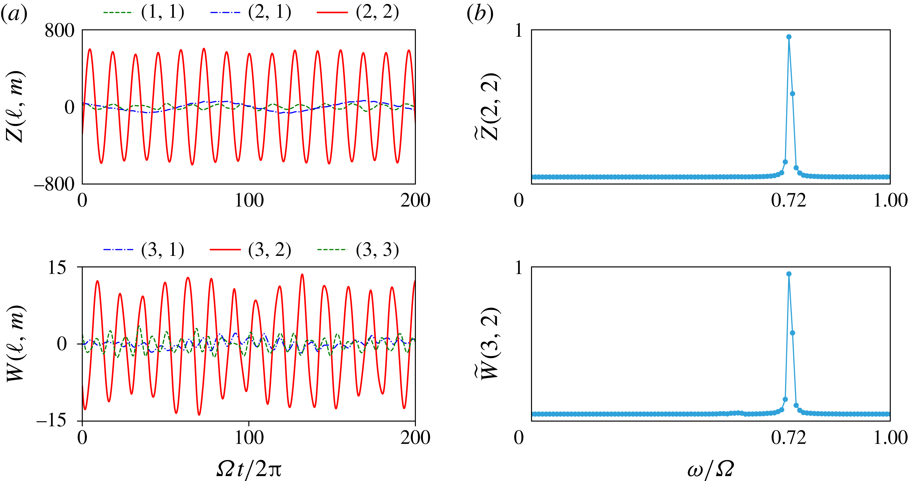
(a) Oscillations of spherical harmonic coefficients of toroidal (
 $Z(\ell ,m)$
) and poloidal (
 $W(\ell ,m)$
) potentials;
 $Z(2,2)$
and
 $W(3,2)$
are the dominant oscillatory coefficients. (b) Fourier transform of time series of coefficients
 $Z(2,2)$
and
 $W(3,2)$
, denoted by tilde, showing a peak in frequency at the same position,
 $\unicode[STIX]{x1D714}/\unicode[STIX]{x1D6FA}=0.72$
. The parameters are
 $E=10^{-4}$
and
 $\unicode[STIX]{x0394}\unicode[STIX]{x1D6FA}/\unicode[STIX]{x1D6FA}=-2$
.

Symmetry of flow field and the corresponding conditions on degree and order of spherical harmonics of poloidal and toroidal potentials.

As an example, let us take the
 $(3,2,0.666)$
inertial mode identified by Wicht (Reference Wicht2014). Figure 4 shows that the toroidal coefficient,
 $Z_{22}$
(
 $l+m=\text{even}$
) is the dominant oscillatory coefficient, while the same is true for the poloidal coefficient
 $W_{32}$
(
 $l+m=\text{odd}$
). The Fourier analyses of the coefficients
 $Z_{22}$
and
 $W_{32}$
show a single strong peak at the same frequency of
 $\unicode[STIX]{x1D714}/\unicode[STIX]{x1D6FA}=0.72$
, where
 $\unicode[STIX]{x1D714}$
is the angular frequency of the Fourier transform. This is shown in figure 4(b).
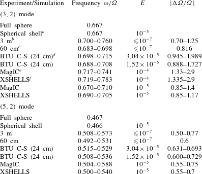
List of the most dominant inertial modes observed and identified, and comparisons with experiments. For simulations at
 $E=10^{-5}$
, the modes seem to occur at similar ranges of
 $|\unicode[STIX]{x0394}\unicode[STIX]{x1D6FA}/\unicode[STIX]{x1D6FA}|$
as all the experiments spanning a huge range of Ekman numbers.

a Using SINGE (Vidal & Schaeffer Reference Vidal and Schaeffer2015).
b From Triana (Reference Triana2011).
c
Frequency ranges from Kelley et al. (Reference Kelley, Triana, Zimmerman, Tilgner and Lathrop2007);
 $\unicode[STIX]{x0394}\unicode[STIX]{x1D6FA}/\unicode[STIX]{x1D6FA}$
values are single representative values from S. Triana.
d From Hoff et al. (Reference Hoff, Harlander, Egbers, Triana, Egbers, Ruck, Leder and Dopheide2016a ,Reference Hoff, Harlander and Triana b ).
e Frequencies determined using spherical harmonics.
f Frequencies determined from spectrograms.
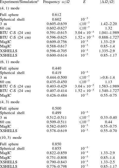
List of less dominant inertial modes and comparisons with experiments and theory. The modes have been identified based on frequency and structures.

a Sources of data same as in table 2.
Tables 2 and 3 give a list of the ‘fast’ inertial modes identified in our simulations and compare it with experimental data as well as data obtained from analytical predictions for a full sphere (e.g. Greenspan Reference Greenspan1968; Zhang et al.
Reference Zhang, Earnshaw, Liao and Busse2001) and eigenmode computations using SINGE. The frequency ranges provided in the tables reflect the fact that the drift frequencies of the modes are not constant but change with differential rotation (
 $\unicode[STIX]{x0394}\unicode[STIX]{x1D6FA}/\unicode[STIX]{x1D6FA}$
) and outer boundary rotation (
 $\unicode[STIX]{x1D6FA}=1/E$
). Differences between MagIC and XSHELLS can be traced back to the slightly different parameters. In some instances the numerical results report an earlier onset of inertial modes, which reflects the easier mode identification using spherical harmonic coefficients.
5 Simulations
To explore the parameter space, we typically keep the rotation rate of the outer boundary constant (constant
 $E$
) and vary the differential rotation (
 $\unicode[STIX]{x0394}\unicode[STIX]{x1D6FA}/\unicode[STIX]{x1D6FA}$
). Simulations at two different Ekman numbers
 $E=10^{-5}$
and
 $10^{-4}$
are performed. We use the results at
 $E=10^{-5}$
to compare directly with those of the experiment, while the
 $E=10^{-4}$
simulations are used to explore a larger range of
 $\unicode[STIX]{x0394}\unicode[STIX]{x1D6FA}/\unicode[STIX]{x1D6FA}$
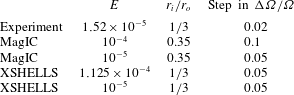
, whose numerical exploration would have been too costly at the lower Ekman number. The details of parameters of the different simulations as well as the experiments are given in table 4.
Parameters for simulations and experiments. The experiments at BTU C-S were run at other Ekman numbers as well; here we provide the one with which we closely compare the simulations.

To reproduce the experimental results and directly compare with them, we produce spectrograms using data from the numerical simulations. For MagIC, time series for the non-axisymmetric part of
 $u_{\unicode[STIX]{x1D719}}$
are stored for eight different points spread out symmetrically in latitude and longitude (
 $\unicode[STIX]{x1D703}=\unicode[STIX]{x03C0}/4,~3\unicode[STIX]{x03C0}/4$
and
 $\unicode[STIX]{x1D719}=0,~\unicode[STIX]{x03C0}/2,~\unicode[STIX]{x03C0},~3\unicode[STIX]{x03C0}/2$
) at
 $r=0.7r_{o}$
. These are stacked after correcting for a phase shift in time. This phase shift has been determined by searching for the time lag providing the highest cross-correlation value. A Fourier transform of the stack yields a spectrum of
 $u_{\unicode[STIX]{x1D719}}$
giving the power in different frequencies. Combining the spectra at different
 $\unicode[STIX]{x0394}\unicode[STIX]{x1D6FA}/\unicode[STIX]{x1D6FA}$
finally provides the spectrogram. For XSHELLS, time-series data are collected for three components of velocity,
 $u_{x}$
,
 $u_{y}$
and
 $u_{z}$
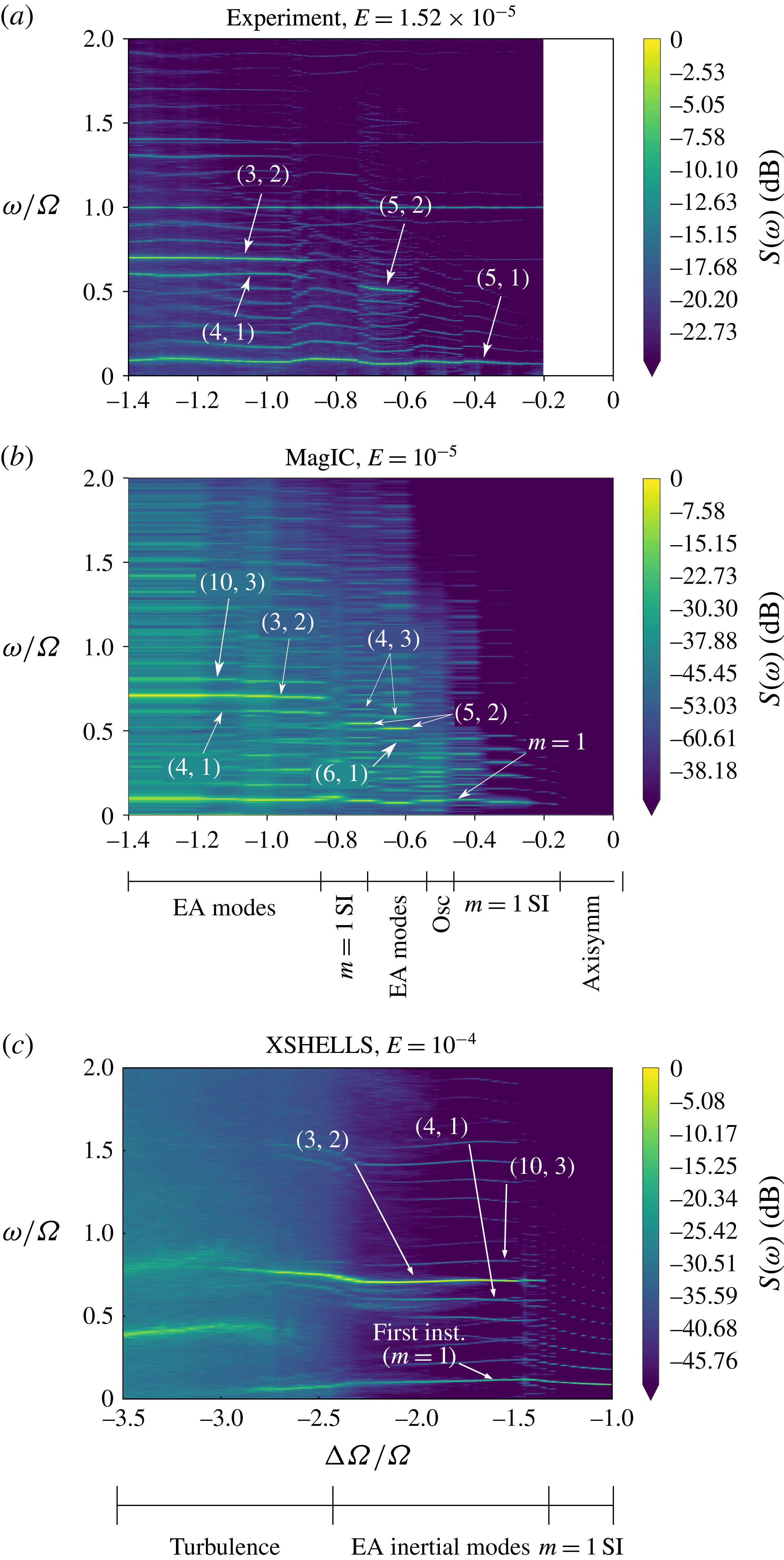
, at eight different points symmetrically spread out in latitude and azimuth. The Fourier transforms of the time series from all points are then averaged to build a spectrogram. The results from the two numerical codes agree with each other, and the spectrograms (figure 5) reproduce the main features observed in the experiment.
Velocity spectrograms obtained from (a) experiments at BTU C-S at
 $E=1.52\times 10^{-5}$
, (b) MagIC at
 $E=10^{-5}$
and (c) XSHELLS at
 $E=10^{-4}$
. The major inertial modes observed have been marked. Note the similar regimes observed in panels (a) and (b). (c) All three regimes observed in the experiments are recovered. Abbreviations: SI
 $=$
Stewartson layer instability, EA
 $=$
equatorially antisymmetric.

The spectrograms and the Fourier analysis of numerical spherical harmonic coefficients (§ 4.2) help us identify the major modes in the solution based on their time dependence. We complement this with an analysis of the spatial structure of the solution, projecting snapshots of the velocity components onto inertial modes of a full sphere. Since inertial modes form an orthogonal system (Greenspan Reference Greenspan1968), one can expand a given velocity field as
 $$\begin{eqnarray}\displaystyle & \displaystyle \boldsymbol{u}=\mathop{\sum }_{j}c_{j}\boldsymbol{Q}_{j}\text{e}^{\text{i}(m_{j}\unicode[STIX]{x1D719}-\unicode[STIX]{x1D714}_{j}t)}, & \displaystyle\end{eqnarray}$$
where
 $\boldsymbol{Q}_{j}\text{e}^{\text{i}(m_{j}\unicode[STIX]{x1D719}-\unicode[STIX]{x1D714}_{j}t)}$
is an inertial mode of the sphere and the coefficients
 $c_{j}$
are given by
 $$\begin{eqnarray}\displaystyle & \displaystyle c_{j}={\displaystyle \frac{\displaystyle \int \boldsymbol{Q}_{j}^{\dagger }\boldsymbol{\cdot }\boldsymbol{u}\,\text{d}V}{\left[\left(\displaystyle \int \boldsymbol{Q}_{j}^{\dagger }\boldsymbol{\cdot }\boldsymbol{Q}_{j}\,\text{d}V\right)\left(\displaystyle \int \boldsymbol{u}\boldsymbol{\cdot }\boldsymbol{u}\,\text{d}V\right)\right]^{1/2}}}, & \displaystyle\end{eqnarray}$$
where
 $^{\dagger }$
represents the complex conjugate and the integrals are performed over the whole spherical shell. We perform such projections for a few different velocity snapshots and then average to obtain the dominant modes over time. To get a better idea of mode contributions to the non-axisymmetric part of the flow, we also project velocity snapshots with the axisymmetric part removed and denote the corresponding coefficients as
 $c_{j}^{\prime }$
. Since the inertial modes are heavily modified by the background flow (§ 6), we cannot expect a perfect representation of the solution by the analytical modes of a sphere. Thus the projection coefficients will never reach one and we would find non-negligible projections on other spurious modes. However, the combination of spatial and temporal analyses yields a clear identification.
We use the methods described above to analyse the different hydrodynamic regimes observed in our simulations, as described below.
5.1 Fundamental
$m=1$
instability

The first instability in the system is a Stewartson layer instability (SI) (e.g. Hollerbach Reference Hollerbach2003) with a well-defined critical
 $(\unicode[STIX]{x0394}\unicode[STIX]{x1D6FA}/\unicode[STIX]{x1D6FA})_{c}$
and azimuthal symmetry
 $m_{c}$
. At
 $E=10^{-4}$
, the first instability has an
 $m=1$
and drifts in azimuth with a frequency
 $\unicode[STIX]{x1D714}/\unicode[STIX]{x1D6FA}=0.086$
(Wicht Reference Wicht2014). This fundamental instability is nearly geostrophic and thus drifts with a very low drift frequency (see § 2.2).
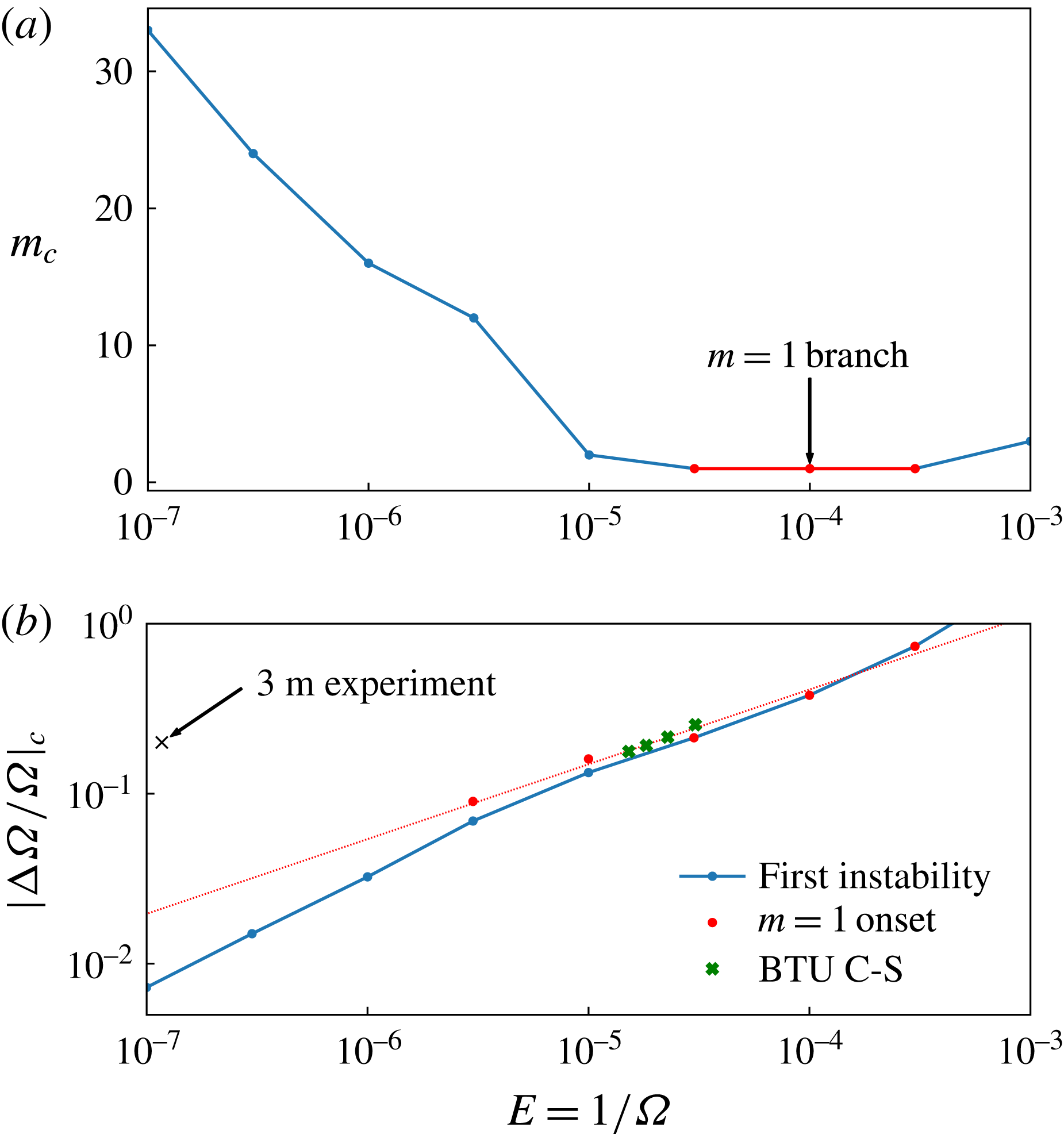
Critical values for onset of first non-axisymmetric instability at different Ekman numbers: (a) the critical wavenumber
 $m$
; (b) the critical differential rotation. Red circles in (b) mark the onset of the fundamental
 $m=1$
mode seen as a secondary instability at low Ekman numbers. A linear extrapolation shows that the 3 m experiment was always supercritical to the
 $m=1$
onset. Green crosses mark the critical
 $|\unicode[STIX]{x0394}\unicode[STIX]{x1D6FA}/\unicode[STIX]{x1D6FA}|$
values determined in experiments at BTU C-S.

The
 $m=1$
fundamental mode at (a)
 $E=10^{-4}$
, (b)
 $E=10^{-5}$
and (c)
 $E=3\times 10^{-6}$
. At
 $E=10^{-4}$
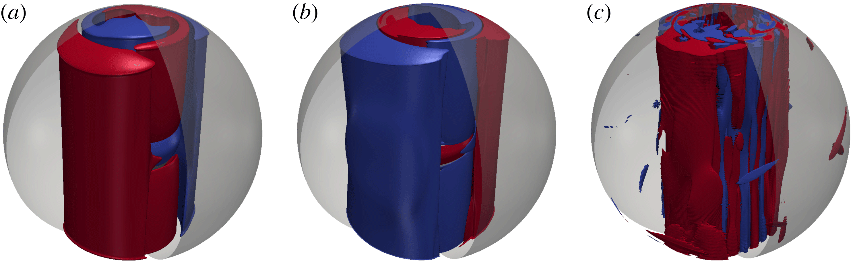
, the mode is the first non-axisymmetric instability to set in. At lower Ekman numbers, it comes in as a secondary instability. Shown here are isosurfaces of non-axisymmetric zonal velocity,
 $u_{\unicode[STIX]{x1D719}}$
, with red (blue) being positive (negative).

At
 $E=10^{-5}$
, even though the first SI has an
 $m_{c}=2$
and
 $(\unicode[STIX]{x0394}\unicode[STIX]{x1D6FA}/\unicode[STIX]{x1D6FA})_{c}=-0.133$
, the same fundamental
 $m=1$
instability sets in as a secondary instability already at
 $\unicode[STIX]{x0394}\unicode[STIX]{x1D6FA}/\unicode[STIX]{x1D6FA}=-0.16$
. Numerical exploration at a lower Ekman number of
 $3\times 10^{-6}$
and the experimental results of Triana (Reference Triana2011) confirm that this mode continues to set in as a secondary instability for smaller Ekman numbers and negative differential rotation. Figure 6(a) shows the critical wavenumber and figure 6(b) the critical differential rotation at onset of the first non-axisymmetric instability for different Ekman numbers for
 $\unicode[STIX]{x0394}\unicode[STIX]{x1D6FA}/\unicode[STIX]{x1D6FA}<0$
. In addition, the onset of the secondary
 $m=1$
instability has also been shown. A linear fit has been used to extrapolate the onset of this instability to lower Ekman numbers. For example, at
 $E=3\times 10^{-6}$
, the first instability sets in for
 $\unicode[STIX]{x0394}\unicode[STIX]{x1D6FA}/\unicode[STIX]{x1D6FA}=-0.0213$
and has a wavenumber of
 $m_{c}=12$
while a secondary
 $m=1$
instability dominates at
 $\unicode[STIX]{x0394}\unicode[STIX]{x1D6FA}/\unicode[STIX]{x1D6FA}=-0.09$
. Figure 7 shows the non-axisymmetric solution at these parameters and clearly illustrates the dominance of the
 $m=1$
but with additional complexity due to the background flow. The dominance of the
 $m=1$
mode was confirmed by a spherical harmonic analysis (§ 4.2). The experimental parameters of the 3 m experiment are clearly located beyond the extrapolated
 $m=1$
onset, which may explain the prominence of this instability in their data (Triana Reference Triana2011). The switchover between
 $m_{c}=1$
and
 $m_{c}=2$
takes place between
 $E=3\times 10^{-5}$
and
 $E=10^{-5}$
. At the parameters of the experiments at BTU C-S,
 $m_{c}=1$
may indeed be the primary instability.
Wicht (Reference Wicht2014) and Hoff et al. (Reference Hoff, Harlander and Triana2016b
) identified the
 $(5,1,-0.068)$
mode as being the most probable candidate for this
 $m=1$
instability, based on a qualitative visual comparison of the spatial structure. However, the observed frequency has an opposite sign (opposite drift direction), which can probably be attributed to the fact that this
 $m=1$
mode is mostly confined to the region inside the TC where the height decreases towards the rotation axis, leading to a negative ‘
 $\unicode[STIX]{x1D6FD}$
effect’ (Schaeffer & Cardin Reference Schaeffer and Cardin2005; Wicht Reference Wicht2014).
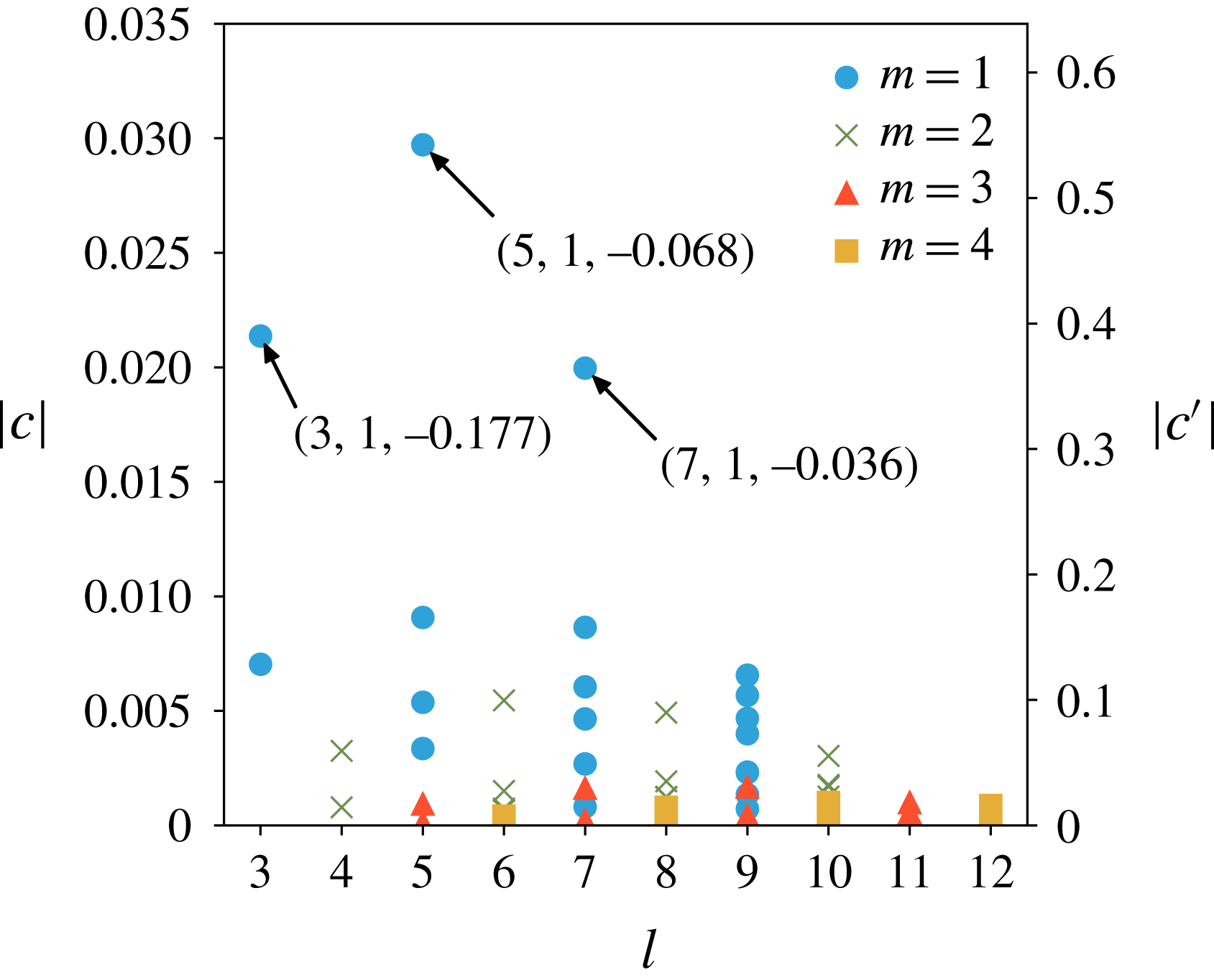
We have calculated the projection coefficients
 $c$
(equation (5.2)) for a wide selection of equatorially symmetric (ES) inertial modes for a more quantitative classification. For this purpose we used a single snapshot at
 $E=10^{-4},\unicode[STIX]{x0394}\unicode[STIX]{x1D6FA}/\unicode[STIX]{x1D6FA}=-0.4$
where the
 $m=1$
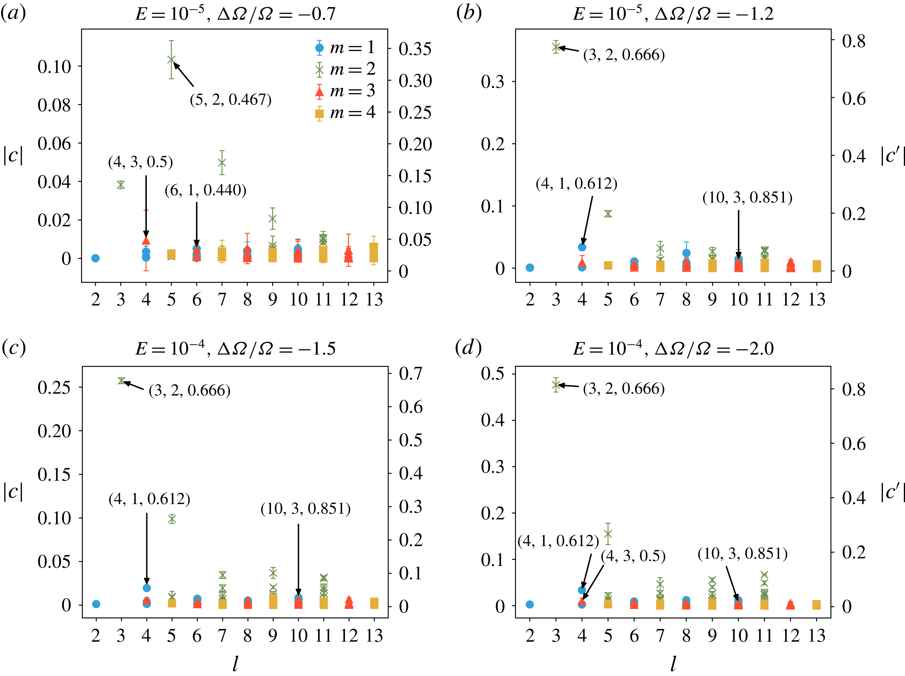
SI mode is simply drifting in azimuth. Since the dynamics is clearly dominated by a simple drift of the different modes, the projection analysis will not depend on the time of the snapshot. Figure 8 summarises the results and illustrates that
 $(5,1,-0.068)$
mode has the largest coefficient
 $c^{\prime }$
between 0.5 and 0.6, considering only the non-axisymmetric flow contribution. The next nearest contenders are the
 $(3,1,-0.177)$
and
 $(7,1,-0.036)$
with not much smaller coefficients between 0.3 and 0.4. In addition to the mismatch in drift direction, this shows that the identification in terms of a single inertial mode remains ambiguous. Therefore, we will refer to it as the
 $m=1$
SI (Stewartson layer instability).
Projection on equatorially symmetric (ES) inertial modes of a velocity snapshot at
 $E=10^{-4},~\unicode[STIX]{x0394}\unicode[STIX]{x1D6FA}/\unicode[STIX]{x1D6FA}=-0.4$
. Here
 $|\cdots |$
represents absolute value and
 $c^{\prime }$
represents the coefficient when the axisymmetric part of the solution has been removed. Different colours and symbols denote different wavenumbers
 $m$
. The dominant modes have been annotated with
 $(l,m,\unicode[STIX]{x1D714}/\unicode[STIX]{x1D6FA})$
. The different points for the same
 $l$
and same colour and symbol (
 $m$
) represent different mode frequencies and structures for the same
 $(l,m)$
combination.

5.2 Inertial modes
As the magnitude of differential rotation is increased, at a certain critical value, ‘fast’ equatorially antisymmetric (EA) inertial modes are excited. However, depending on the Ekman number, one obtains a different set of modes and a slightly different behaviour of the kinetic energy at onset.
Analysing the MagIC results shows that, at
 $E=10^{-5}$
, the equatorial symmetry is broken at
 $\unicode[STIX]{x0394}\unicode[STIX]{x1D6FA}/\unicode[STIX]{x1D6FA}=-0.35$
, but the EA kinetic energy remains too low to identify any underlying mode. A larger differential rotation leads to oscillations in the kinetic energy, attributable to nonlinear interactions between different modes. At
 $\unicode[STIX]{x0394}\unicode[STIX]{x1D6FA}/\unicode[STIX]{x1D6FA}=-0.55$
, the first clear onset of EA inertial modes takes place. The dominant mode is the
 $(5,2,0.467)$
mode seen as a clear ‘bright’ line in the spectrograms of the experiment as well as the simulations (figure 5
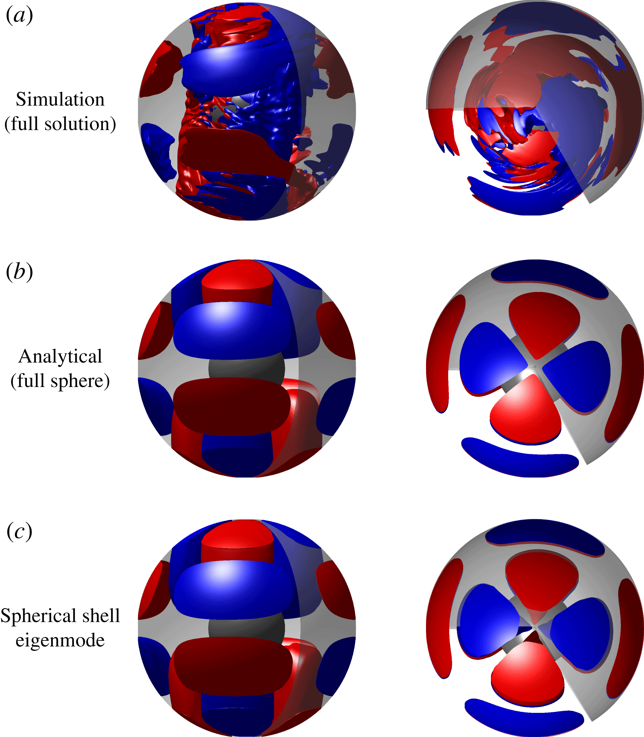
a,b). Figure 9 compares a velocity snapshot at
 $\unicode[STIX]{x0394}\unicode[STIX]{x1D6FA}/\unicode[STIX]{x1D6FA}=-0.6$
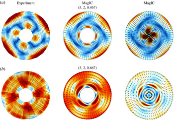
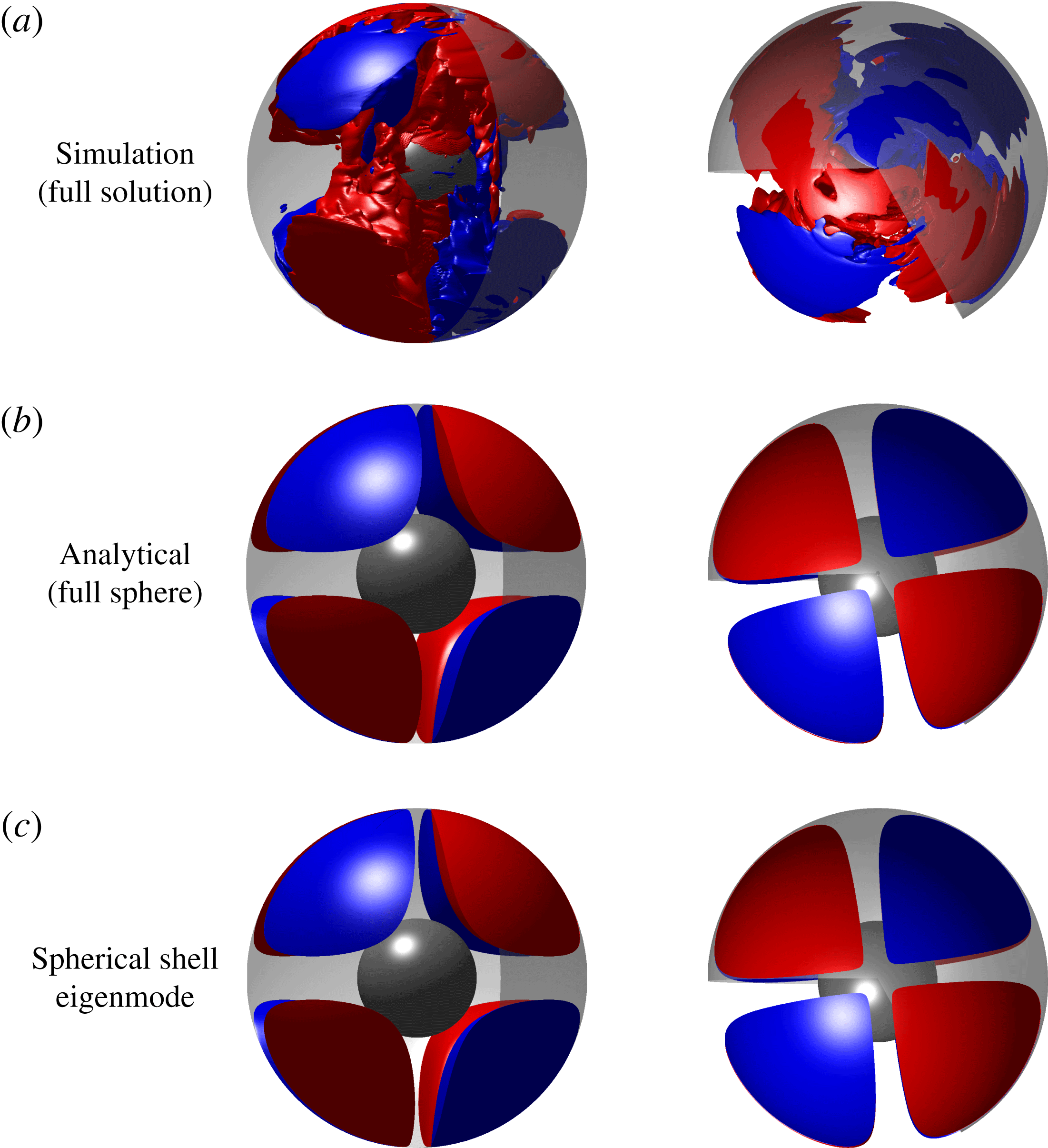
with eigenmodes of a sphere and a spherical shell. While the full numerical solution looks similar to the eigenmodes, it has also been evidently modified by the background flow due to the shear on and inside the TC. Figure 10(a) compares the
 $m=2$
equatorially antisymmetric contribution of the MagIC simulations to that of the reconstructed velocity from PIV measurements in the experiments. The PIV data have been filtered to retain only a narrow frequency band and cover only part of the planar circle (see figure 2(b) in Hoff et al. (Reference Hoff, Harlander, Egbers, Triana, Egbers, Ruck, Leder and Dopheide2016a
)). The filtering process of the numerical solution and the experiments guarantees that both screen out everything else but the
 $(5,2,0.467)$
mode. The full circle view of the experimental results shown in figure 10 had to be reconstructed from several measurements, leaving a gap in the centre. The experimental flow reconstruction errors are estimated to be up to 15 % in the centre of the field of view and up to 25 % near corners and edges (Hoff et al.
Reference Hoff, Harlander, Egbers, Triana, Egbers, Ruck, Leder and Dopheide2016a
). These limitations along with the different scaling used in the numerical simulation complicates a direct comparison. However, both agree on a qualitative level. The dominance of the
 $(5,2,0.467)$
mode is also testified by its relatively large projection coefficient, as illustrated in figure 12(a).
Comparison of flow structures between simulation (a), analytical prediction for a full sphere (b) based on Zhang et al. (Reference Zhang, Earnshaw, Liao and Busse2001) and spherical shell eigenmode computed using SINGE (c) for the
 $(5,2)$
mode at
 $E=10^{-5}$
,
 $\unicode[STIX]{x0394}\unicode[STIX]{x1D6FA}/\unicode[STIX]{x1D6FA}=-0.6$
. Shown here are isosurfaces of non-axisymmetric cylindrically radial velocity (
 $u_{s}$
) of a snapshot of the solution. Red is positive (outwards) while blue is negative (inwards). Note that no filtering has been performed on the solution. The whole solution is dominated by this mode at these parameters. The similarities are self-evident.

Comparison of
 $z$
-slices of velocity magnitudes from experiments and simulations for (a) the
 $(5,2,0.467)$
mode and (b) the
 $(3,2,0.667)$
mode. The experimental data have been taken at
 $z/r_{o}=1/3$
, while the simulation data have been shown at
 $z/r_{o}=0.35$
with the centre of the spheres as the origin. The second column shows a slice from a MagIC simulation without a central part and saturated colours so as to bring out the similarities better. The third column shows the full slice from the simulation. The structures look very similar for both modes. For the
 $(5,2,0.467)$
mode the data have been taken at
 $\unicode[STIX]{x0394}\unicode[STIX]{x1D6FA}/\unicode[STIX]{x1D6FA}=-0.68$
for the experiment and at
 $\unicode[STIX]{x0394}\unicode[STIX]{x1D6FA}/\unicode[STIX]{x1D6FA}=-0.7$
for the simulation. For the
 $(3,2)$
mode, the corresponding numbers are
 $\unicode[STIX]{x0394}\unicode[STIX]{x1D6FA}/\unicode[STIX]{x1D6FA}=-1.11$
and
 $\unicode[STIX]{x0394}\unicode[STIX]{x1D6FA}/\unicode[STIX]{x1D6FA}=-1.1$
, respectively. Colours and arrow lengths represent velocity magnitudes – horizontal velocity for experiments and total velocity for simulations. The arrows also indicate velocity direction.

Same as figure 9 for the
 $(3,2)$
mode at
 $E=10^{-5}$
,
 $\unicode[STIX]{x0394}\unicode[STIX]{x1D6FA}/\unicode[STIX]{x1D6FA}=-1$
.

Projection of velocity snapshots on equatorially antisymmetric (EA) inertial modes of a sphere at different parameters. The major modes have been annotated using
 $(l,m,\unicode[STIX]{x1D714}/\unicode[STIX]{x1D6FA})$
. Here
 $c^{\prime }$
represents the projection coefficient of the snapshot with the axisymmetric part removed. Error bars show the temporal standard deviation in
 $|c^{\prime }|$
. We used the following number of snapshots for computing the time average: (a) five, (b) five, (c) seven and (d) six.

Table 2 compares the frequencies of the
 $(5,2,0.467)$
mode found in different experimental set-ups as well as the two numerical simulations presented here and the eigenvalues for a full sphere and a spherical shell. The two eigenvalues agree perfectly. Numerical and experimental values are nearly in agreement with each other but show a slightly larger frequency than the eigenvalue predictions. A possible reason is the effect of the background flow, which is completely ignored in eigenmode computations. The dependence on differential rotation will be discussed in § 6. Since the values in table 2 span four decades in Ekman number, the dependence of the frequency on Ekman number can only be weak.
Besides the two most dominant lines in the spectrogram for the
 $m=1$
SI and the
 $(5,2,0.467)$
modes, there are several other lines which are less dominant but nevertheless clearly visible against the background. Prominent among these are two ‘side branches’ around
 $\unicode[STIX]{x1D714}/\unicode[STIX]{x1D6FA}=0.5$
and
 $\unicode[STIX]{x1D714}/\unicode[STIX]{x1D6FA}=0.44$
, identified as the
 $(4,3,0.5)$
and an
 $m=1$
EA mode, respectively. The latter is difficult to identify unambiguously as a single inertial mode due to its complex structure. However, we identify it as the
 $(6,1,0.44)$
since the frequency is close (as seen in table 3) and the respective projection coefficient is the largest of all
 $m=1$
EA modes (figure 12
a). Since the time behaviour is more complex, the calculation of the projection coefficients now relies on several snapshots. Figure 12 shows mean coefficients and illustrates the standard deviation with error bars. Note that table 3 also shows a strong influence of the background flow on the frequency, as will be discussed in § 6. Furthermore, MagIC results suggest an earlier onset at around
 $\unicode[STIX]{x0394}\unicode[STIX]{x1D6FA}/\unicode[STIX]{x1D6FA}=-0.55$
, while in the BTU C-S experiments, the mode was not detected before
 $\unicode[STIX]{x0394}\unicode[STIX]{x1D6FA}/\unicode[STIX]{x1D6FA}=-1.54$
. A possible explanation for this discrepancy is the fact that the mode is difficult to identify in the experiment because of its complex structure and low amplitude.
However, at
 $\unicode[STIX]{x0394}\unicode[STIX]{x1D6FA}/\unicode[STIX]{x1D6FA}=-0.8$
these modes disappear, the EA kinetic energy decreases significantly and the
 $m=1$
SI mode again becomes the dominant large-scale structure. This regime is followed by an onset of a different set of EA modes at
 $\unicode[STIX]{x0394}\unicode[STIX]{x1D6FA}/\unicode[STIX]{x1D6FA}=-0.85$
consisting of the dominant
 $(3,2,0.667)$
mode with ‘side branches’ of
 $(4,1,0.612)$
and
 $(10,3,0.851)$
modes, as seen in the spectrograms in figures 5(a) and 5(b). The visual comparison of a numerical snapshot at
 $\unicode[STIX]{x0394}\unicode[STIX]{x1D6FA}/\unicode[STIX]{x1D6FA}=-1$
with eigenmodes of a full sphere and a spherical shell in figure 11 clearly attests to the large
 $(3,2,0.667)$
contribution. Figure 10(b) shows the similarity of the respective mode in the simulation and experiment. The projection coefficients shown in figure 12(b) quantify the dominance of the
 $(3,2,0.667)$
mode. The projection coefficients substantiate that the
 $(3,2,0.667)$
contribution amounts to about 80 % of the non-axisymmetric solution. Once again the mode identification is challenging for the subdominant modes, but a combined analysis of projection coefficients and frequency matching helps us single out these modes as the best candidates. Table 2 lists the frequencies of the
 $(3,2,0.667)$
mode eigenmodes for a sphere and a spherical shell as well as for the solutions observed in simulations and experiments. The deviations from the eigenvalues are probably due to the effect of background flow, as will be discussed in § 6. These EA modes along with the
 $m=1$
SI remain the dominant modes till the largest differential rotation magnitude that could be afforded using existing computational resources. The limits were
 $\unicode[STIX]{x0394}\unicode[STIX]{x1D6FA}/\unicode[STIX]{x1D6FA}=-1.4$
for MagIC and
 $\unicode[STIX]{x0394}\unicode[STIX]{x1D6FA}/\unicode[STIX]{x1D6FA}=-1.17$
for XSHELLS.
However, at an Ekman number of
 $E=10^{-4}$
we could run simulations with larger differential rotation magnitudes and consequently venture into the turbulent regime. At this higher Ekman number, a similar onset of EA inertial modes is observed. However, unlike at
 $E=10^{-5}$
, these modes remain dominant right up to the onset of turbulence. After the onset of the
 $m=1$
SI mode at
 $\unicode[STIX]{x0394}\unicode[STIX]{x1D6FA}/\unicode[STIX]{x1D6FA}=-0.379$
, we find kinetic energy oscillations due to nonlinear mode interactions starting at
 $\unicode[STIX]{x0394}\unicode[STIX]{x1D6FA}/\unicode[STIX]{x1D6FA}=1.25$
. These give way to EA inertial modes at
 $\unicode[STIX]{x0394}\unicode[STIX]{x1D6FA}/\unicode[STIX]{x1D6FA}=-1.33$
, determined using lower steps in
 $\unicode[STIX]{x0394}\unicode[STIX]{x1D6FA}/\unicode[STIX]{x1D6FA}$
. The
 $(3,2,0.667)$
mode is the most dominant mode accompanied by ‘side branches’ of
 $(4,1,0.612)$
and
 $(10,3,0.851)$
modes. They can be seen as three ‘bright’ lines in the spectrogram (figure 5
c) around
 $\unicode[STIX]{x1D714}/\unicode[STIX]{x1D6FA}=0.7,~0.6,~0.85$
, respectively. In the projections shown in figures 12(c) and 12(d), the
 $(3,2,0.667)$
,
 $(4,1,0.612)$
and
 $(10,3,0.851)$
modes are seen to be dominant. The modes mentioned above will hereafter be referred to using only the indices
 $(l,m)$
, as only a single mode for an
 $(l,m)$
combination is observed.
Tables 2 and 3 compare the frequencies and
 $\unicode[STIX]{x0394}\unicode[STIX]{x1D6FA}/\unicode[STIX]{x1D6FA}$
ranges of the observed inertial modes in our simulations with those observed in past experiments. It is evident that the observations of these modes are very robust and similar modes are seen across several orders of magnitudes in Ekman number.
At
 $E=10^{-4}$
, the transition to turbulence takes place around
 $\unicode[STIX]{x0394}\unicode[STIX]{x1D6FA}/\unicode[STIX]{x1D6FA}=-2.3$
, which is larger in magnitude as compared to the value of
 $\unicode[STIX]{x0394}\unicode[STIX]{x1D6FA}/\unicode[STIX]{x1D6FA}=-1.73$
at
 $E=1.52\times 10^{-5}$
, as found by Hoff et al. (Reference Hoff, Harlander and Triana2016b
).
The frequencies of the dominant
 $(3,2)$
and the
 $m=1$
SI modes are more strongly influenced by the background flow, including a sudden jump in the frequency of the
 $(3,2)$
mode, similar to observations by Hoff et al. (Reference Hoff, Harlander and Triana2016b
). At around
 $\unicode[STIX]{x0394}\unicode[STIX]{x1D6FA}/\unicode[STIX]{x1D6FA}=-2.7$
, a new equatorially symmetric mode with
 $m=2$
sets in but the corresponding inertial mode has not yet been determined. The turbulent regime, though very interesting, is beyond the scope of the present study and will not be discussed further.
6 Effect of background flow on inertial modes
Tables 2 and 3 show that for some cases the frequencies of the inertial modes in the simulations as well as in the experiments (BTU C-S, 3 m, 60 cm) match the theoretical predictions very closely, while for other cases, like for the
 $(4,3)$
mode, the difference can be as large as 40 %. The comparison of eigenvalues for a spherical shell and a full sphere in tables 2 and 3 show that the presence of an inner sphere has a relatively small effect, at most 5 % seen for the
 $(6,1)$
mode. However, the simulations show that the modes are distorted inside and close to the TC, which probably goes along with the change in eigenfrequency. Another possible cause for the frequency difference is advection due to the background flow (Schaeffer & Cardin Reference Schaeffer and Cardin2005; Wicht Reference Wicht2014; Hoff et al.
Reference Hoff, Harlander and Triana2016b
).
To explore this, we artificially excite inertial modes at different
 $\unicode[STIX]{x0394}\unicode[STIX]{x1D6FA}/\unicode[STIX]{x1D6FA}$
using MagIC. Following Rieutord et al. (Reference Rieutord, Triana, Zimmerman and Lathrop2012), we impose an artificial outer boundary forcing with a velocity
 $$\begin{eqnarray}\displaystyle & \displaystyle \boldsymbol{u}(\unicode[STIX]{x1D703},\unicode[STIX]{x1D719})=\left(\displaystyle \frac{1}{\sin \unicode[STIX]{x1D703}}\displaystyle \frac{\unicode[STIX]{x2202}Y_{m}^{m}}{\unicode[STIX]{x2202}\unicode[STIX]{x1D719}}\hat{\boldsymbol{e}}_{\unicode[STIX]{x1D703}}-\displaystyle \frac{\unicode[STIX]{x2202}Y_{m}^{m}}{\unicode[STIX]{x2202}\unicode[STIX]{x1D703}}\hat{\boldsymbol{e}}_{\unicode[STIX]{x1D719}}\right)\text{e}^{-\text{i}\unicode[STIX]{x1D714}t}, & \displaystyle\end{eqnarray}$$
where
 $\hat{\boldsymbol{e}}$
represent unit vectors in
 $\unicode[STIX]{x1D703}$
and
 $\unicode[STIX]{x1D719}$
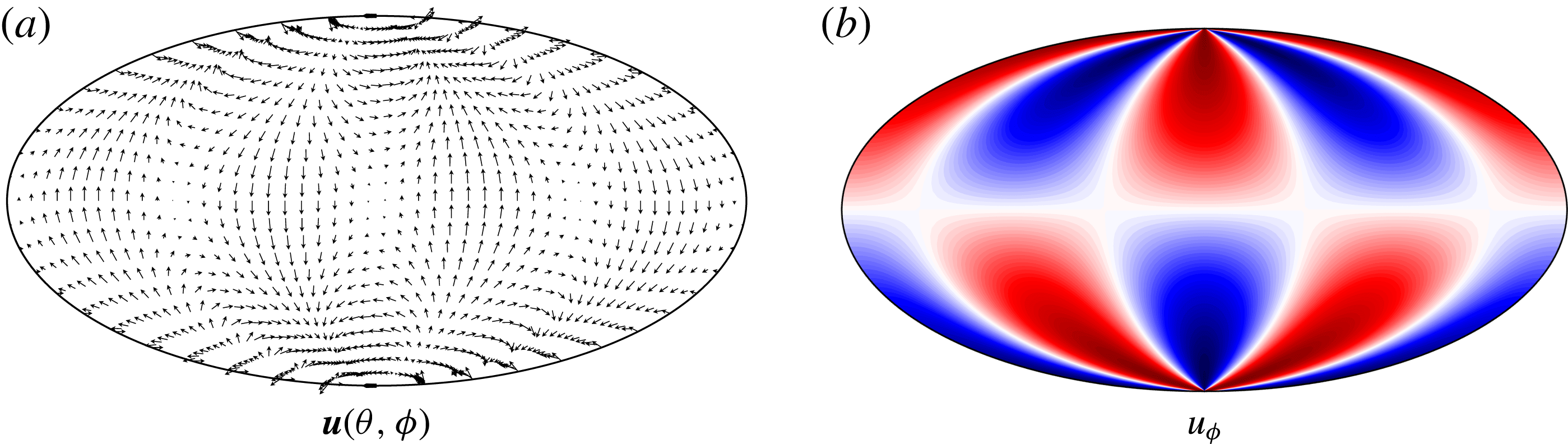
directions. The forcing velocity field for
 $m=2$
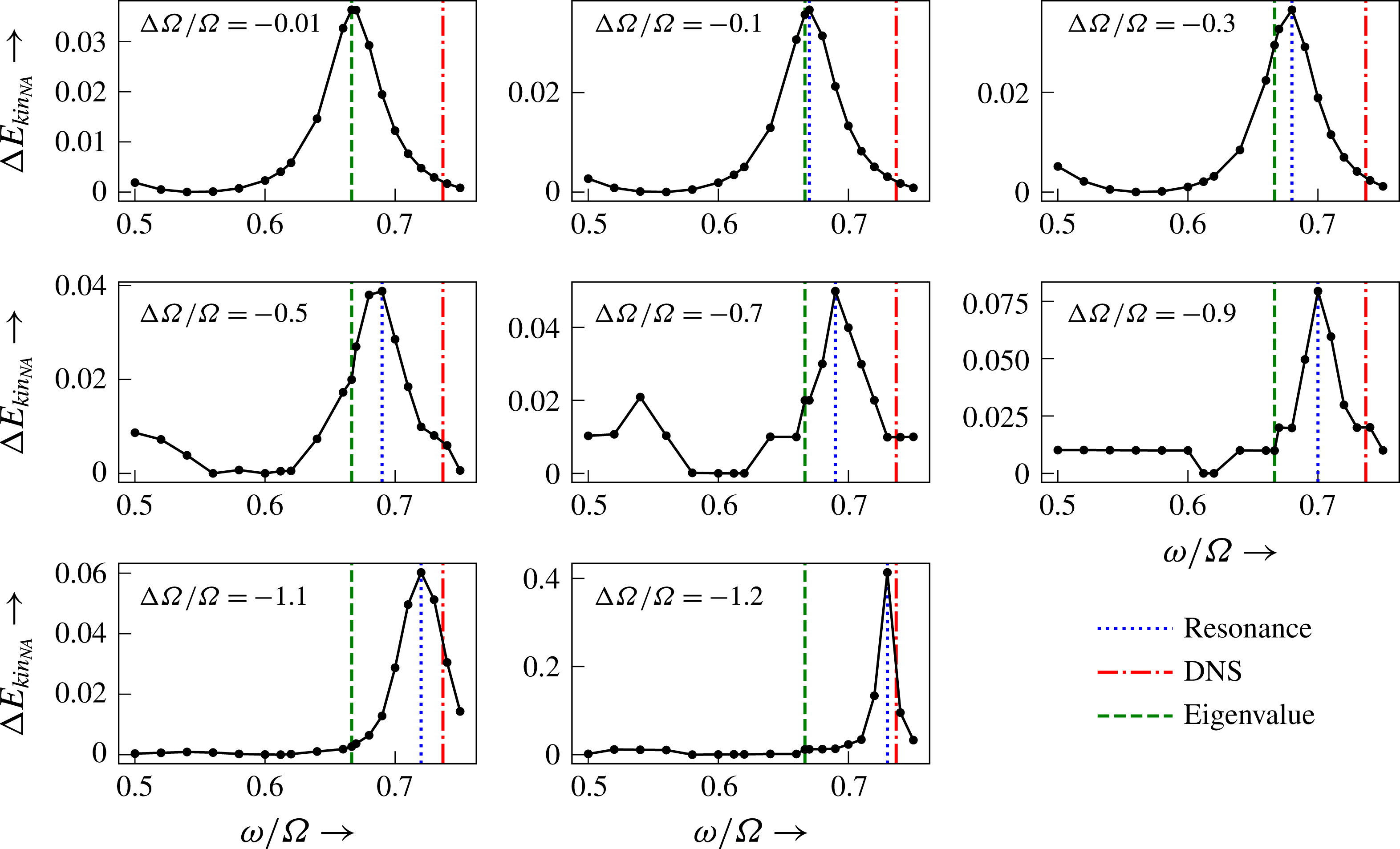
is shown in figure 13, where the equatorially antisymmetric nature of the forcing is clearly visible. For a fixed
 $\unicode[STIX]{x0394}\unicode[STIX]{x1D6FA}/\unicode[STIX]{x1D6FA}$
, we artificially excite an
 $m=2$
mode at different frequencies and determine the normal mode resonance.
Boundary forcing
 $\boldsymbol{u}(\unicode[STIX]{x1D703},\unicode[STIX]{x1D719})$
for
 $m=2$
: (a) the vector
 $\boldsymbol{u}$
on the outer boundary, and (b) the zonal component, red being prograde and blue retrograde.

Figure 14 shows the resonant
 $(3,2)$
mode excitation at eight different
 $\unicode[STIX]{x0394}\unicode[STIX]{x1D6FA}/\unicode[STIX]{x1D6FA}$
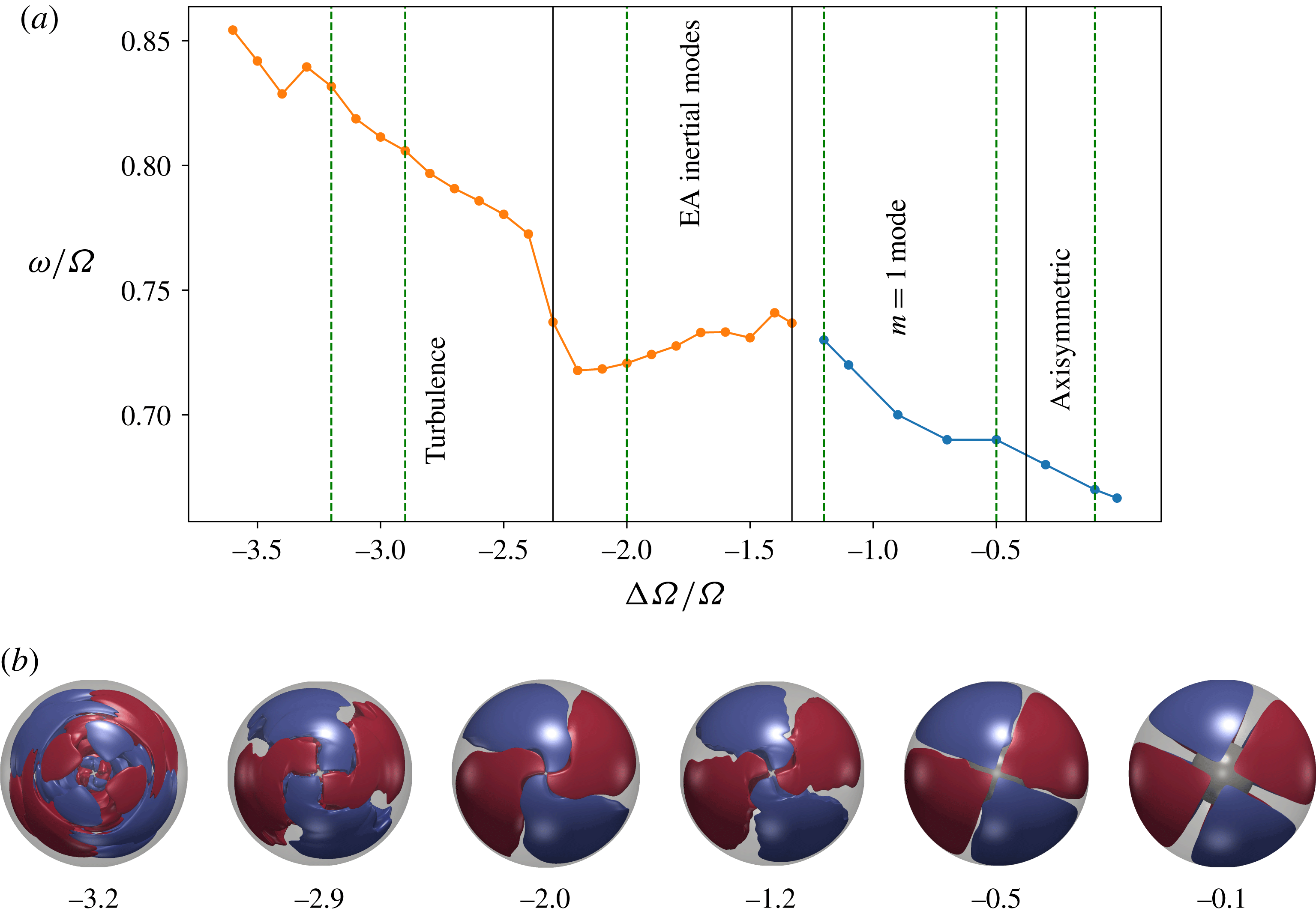
. The dependence of the resonance frequency on
 $\unicode[STIX]{x0394}\unicode[STIX]{x1D6FA}/\unicode[STIX]{x1D6FA}$
is compiled in figure 15. For vanishingly small
 $\unicode[STIX]{x0394}\unicode[STIX]{x1D6FA}/\unicode[STIX]{x1D6FA}$
, we recover the sphere/shell eigenvalues. Increasing
 $|\unicode[STIX]{x0394}\unicode[STIX]{x1D6FA}/\unicode[STIX]{x1D6FA}|$
, the frequency rises and gradually approaches that of the
 $(3,2)$
mode found at its natural onset at
 $\unicode[STIX]{x0394}\unicode[STIX]{x1D6FA}/\unicode[STIX]{x1D6FA}=-1.33$
. Figure 15 also illustrates how the frequency changes with
 $\unicode[STIX]{x0394}\unicode[STIX]{x1D6FA}/\unicode[STIX]{x1D6FA}$
after the mode naturally onsets (orange line, no artificial excitation). We find that the frequency of the mode has a small decrease with increasing
 $|\unicode[STIX]{x0394}\unicode[STIX]{x1D6FA}/\unicode[STIX]{x1D6FA}|$
with a sudden jump at the onset of turbulence. Hoff et al. (Reference Hoff, Harlander and Triana2016b
) speculate that this sudden jump is caused by a Doppler effect since the turbulence causes an increase of the background flow velocity outside the TC where the
 $(3,2)$
mode mostly lives. However, a Doppler effect cannot explain the much weaker changes for other
 $\unicode[STIX]{x0394}\unicode[STIX]{x1D6FA}/\unicode[STIX]{x1D6FA}$
, and in particular the decrease in frequency before the onset of the turbulence, since the background flow and the mode drift are in the same direction. Here, the change in eigenfrequency is a more likely explanation. The small gap in between the two lines is due to the onset of the kinetic energy oscillations at
 $\unicode[STIX]{x0394}\unicode[STIX]{x1D6FA}/\unicode[STIX]{x1D6FA}=-1.25$
, which prevented us from going closer to the onset value of the inertial mode.
Influence of background rotation on inertial mode frequency for mode
 $(3,2)$
in Greenspan notation, at
 $E=10^{-4}$
. For very small differential rotation, we recover the analytical prediction for a full sphere. Increase of
 $\unicode[STIX]{x0394}\unicode[STIX]{x1D6FA}/\unicode[STIX]{x1D6FA}$
to more negative values changes the normal mode frequency and shifts it towards the value we observe in simulations. The onset of inertial modes for simulations at this Ekman number is at
 $\unicode[STIX]{x0394}\unicode[STIX]{x1D6FA}/\unicode[STIX]{x1D6FA}=-1.33$
.

(a) Shows change in normal mode frequency versus
 $\unicode[STIX]{x0394}\unicode[STIX]{x1D6FA}/\unicode[STIX]{x1D6FA}$
for the
 $(3,2)$
mode at
 $E=10^{-4}$
. The blue line denotes artificially excited mode while the orange line shows the mode frequency after it has naturally onset. The frequency changes from the analytical value for a full sphere to the one found in our simulations. (b) Shows top views (
 $+z$
view) of
 $m=2$
equatorially antisymmetric cylindrically radial velocity illustrating the filtered
 $(3,2)$
mode for different
 $\unicode[STIX]{x0394}\unicode[STIX]{x1D6FA}/\unicode[STIX]{x1D6FA}$
.

The lower panel of figure 15 illustrates the effect of background flow on the structure of the
 $(3,2)$
inertial mode. Until
 $\unicode[STIX]{x0394}\unicode[STIX]{x1D6FA}/\unicode[STIX]{x1D6FA}=-1.2$
, the mode is artificially excited while the other panels illustrate the naturally excited mode. With increase in differential rotation magnitude, the mode is progressively distorted. Beyond
 $\unicode[STIX]{x0394}\unicode[STIX]{x1D6FA}/\unicode[STIX]{x1D6FA}=-0.5$
, the regions inside and outside the TC appear twisted against each other due to the background shear flow. For
 $\unicode[STIX]{x0394}\unicode[STIX]{x1D6FA}/\unicode[STIX]{x1D6FA}<0$
, the region inside the TC rotates retrograde with respect to the region outside. In the turbulent regime, the background flow is modified (Hoff et al.
Reference Hoff, Harlander and Triana2016b
), leading to a more complex structure.
Internal shear layers are a characteristic feature of inertial modes (e.g. Stewartson & Rickard Reference Stewartson and Rickard1969). In an inviscid system without background flow, they emanate from critical latitudes for which
 $\cos \unicode[STIX]{x1D703}=\unicode[STIX]{x1D714}/2\unicode[STIX]{x1D6FA}$
, are oriented along the characteristics of the inertial wave equation, and always maintain the same angle of
 $\cos ^{-1}(\unicode[STIX]{x1D714}/2\unicode[STIX]{x1D6FA})$
with respect to the rotation axis. Since they are so thin, they have only been detected once in spherical Couette experiments (Triana Reference Triana2011) and only for the ‘spin-over’ mode, which is not present in our system.
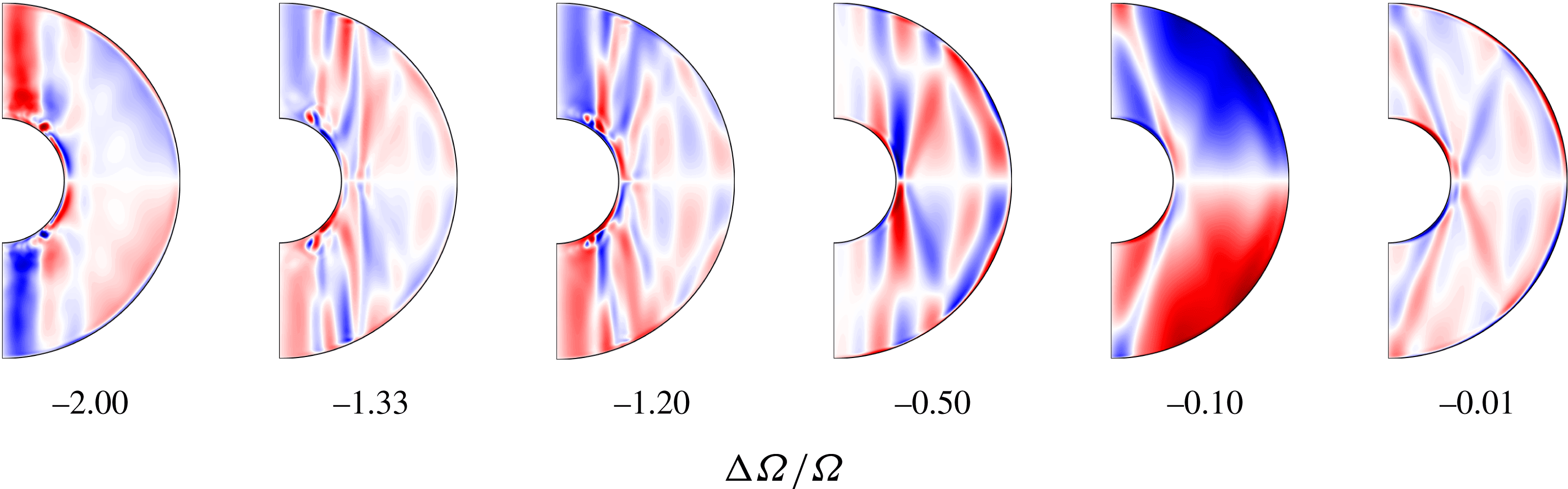
Meridional slices of zonal velocity
 $u_{\unicode[STIX]{x1D719}}$
of the filtered
 $(3,2)$
mode as
 $\unicode[STIX]{x0394}\unicode[STIX]{x1D6FA}/\unicode[STIX]{x1D6FA}$
changes. The internal shear layers seen initially seem to get aligned more and more with the rotation axis as the magnitude of differential rotation increases.

To illustrate how the shear layers change with differential rotation, we filter out the
 $(3,2)$
mode and compare meridional sections of zonal velocity
 $u_{\unicode[STIX]{x1D719}}$
in figure 16. With no differential rotation, the internal shear layers emanate as straight lines from the predicted critical latitudes at the expected critical angle. However, as one increases the differential rotation magnitude, the shear layers that overlap with the Stewartson shear layer are modified and get aligned with the Stewartson layer. At large differential rotation magnitudes, the internal shear layers are further modified and become weaker. For
 $\unicode[STIX]{x0394}\unicode[STIX]{x1D6FA}/\unicode[STIX]{x1D6FA}=-2$
, they seem to have vanished further away from the TC.
7 Triadic interactions
7.1 Theoretical background
The phenomenon of triadic resonance may appear in any physical problem involving nonlinear wave interactions. Coupled harmonic oscillators, photon decay and waves in plasma (see e.g Bellan Reference Bellan2008) are just a few examples. In a geophysical context, they have been studied in relation to internal waves in the oceans (McComas & Bretherton Reference McComas and Bretherton1977) and resonant interactions of Rossby waves (Pedlosky Reference Pedlosky1987) and their instability (Zhang & Pedlosky Reference Zhang and Pedlosky2007). Triadic resonances are also observed when a flow becomes unstable to inertial modes. Examples of such instabilities are the elliptical and shear instabilities in precession (Kerswell Reference Kerswell1993).
It can be shown (see appendix A) that the nonlinear interaction of two inertial modes
 $\boldsymbol{Q}_{1}\text{e}^{\text{i}(m_{1}\unicode[STIX]{x1D719}-\unicode[STIX]{x1D714}_{1}t)}$
and
 $\boldsymbol{Q}_{2}\text{e}^{\text{i}(m_{2}\unicode[STIX]{x1D719}-\unicode[STIX]{x1D714}_{2}t)}$
can resonantly excite a third mode
 $\boldsymbol{Q}_{k}\text{e}^{\text{i}(m_{k}\unicode[STIX]{x1D719}-\unicode[STIX]{x1D714}_{k}t)}$
if the following conditions are met:
(i) The wavenumbers have to match
(7.1)$$\begin{eqnarray}\displaystyle & \displaystyle m_{k}=m_{1}\pm m_{2}. & \displaystyle\end{eqnarray}$$
(ii) The frequencies have to fulfil
(7.2)$$\begin{eqnarray}\displaystyle & \displaystyle \unicode[STIX]{x1D714}_{k}=\unicode[STIX]{x1D714}_{1}\pm \unicode[STIX]{x1D714}_{2}. & \displaystyle\end{eqnarray}$$
(iii) The integral over
$\text{d}\unicode[STIX]{x1D70F}=r^{2}\sin \unicode[STIX]{x1D703}\,\text{d}r\,\text{d}\unicode[STIX]{x1D703}$
provides additional selection rules. An obvious one concerns the equatorial symmetry. The product of two vector fields of opposite equatorial symmetry vanishes when integrated over volume. Thus, the integral over
$\text{d}\unicode[STIX]{x1D70F}$
is non-zero only when
$\boldsymbol{Q}_{k}^{\dagger }$
and hence
$\boldsymbol{Q}_{k}$
has the same equatorial symmetry as the nonlinear terms involving
$\boldsymbol{Q}_{1}$
and
$\boldsymbol{Q}_{2}$
. If
$\boldsymbol{Q}_{1}$
and
$\boldsymbol{Q}_{2}$
have opposite equatorial symmetries, then
$\boldsymbol{Q}_{k}$
has to be equatorially antisymmetric. If both of them possess the same equatorial symmetry,
$\boldsymbol{Q}_{k}$
has to be equatorially symmetric.(iv) The
$\text{d}\unicode[STIX]{x1D70F}$
integral may also define additional constraints for the radial and latitudinal structure that are not explored here.





7.2 Triadic resonances in the inertial mode regime
All the identified ‘fast’ inertial modes form pairwise triadic resonances with the fundamental
 $m=1$
SI mode. For example, at
 $E=10^{-4}$
, we identify the triads
 $[m=1\;\text{SI},(3,2),(4,1)]$
and
 $[m=1\;\text{SI},(10,3),(3,2)]$
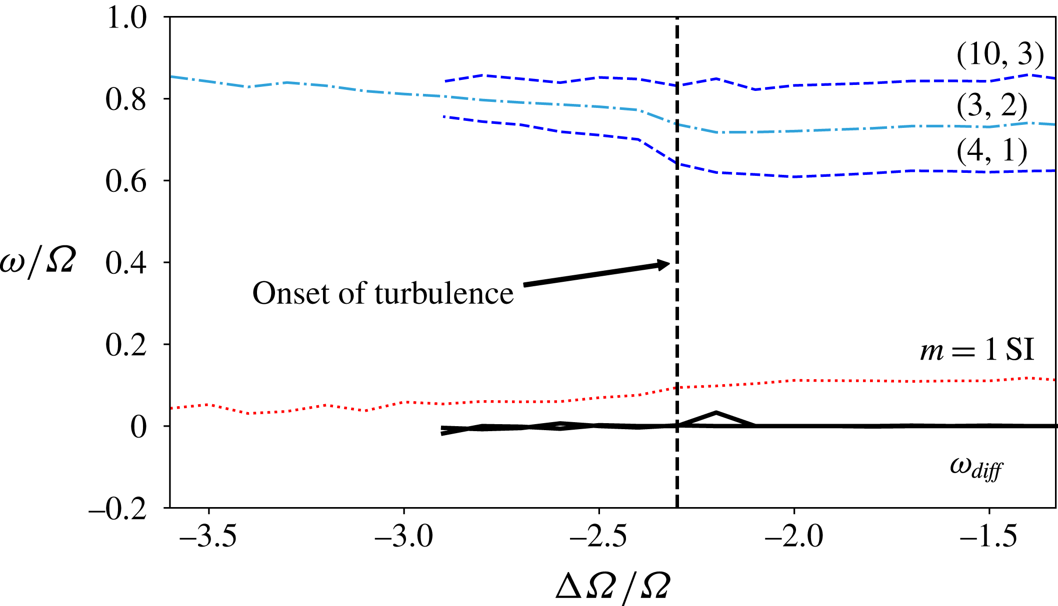
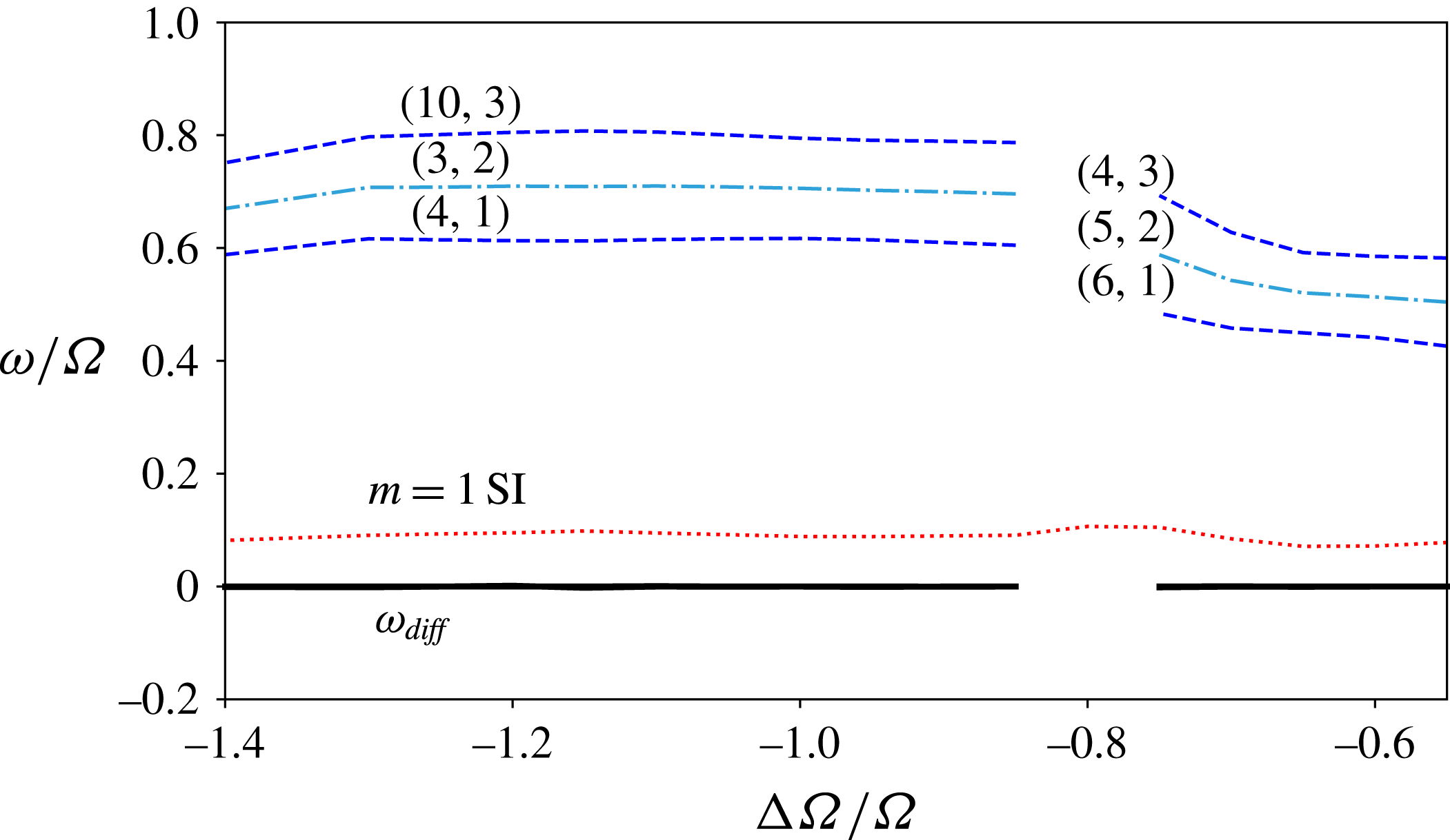
. The triads obviously fulfil the wavenumber criterion and figure 17 confirms that their frequencies indeed add up to nearly zero. As for spherical harmonics, inertial modes are equatorially symmetric (antisymmetric) when the difference
 $l-m$
is even (odd). The equatorial symmetry criterion is thus also fulfilled.
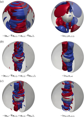
Figure 18 shows the three-dimensional structure of the nonlinear advective acceleration of the triad
 $[(3,2),(4,1),m=1\;\text{SI}]$
in the left column. This is compared with the effective acceleration of the mode with the respective wavenumber, frequency and equatorial symmetry on the right. While the driving has a richer radial and latitudinal structure, only the simpler modes are resonantly driven.
Triadic resonances at
 $E=10^{-4}$
. Here
 $\unicode[STIX]{x1D714}_{diff}$
refers to the lines of the differences:
 $\unicode[STIX]{x1D714}_{(3,2)}-\unicode[STIX]{x1D714}_{(4,1)}-\unicode[STIX]{x1D714}_{m=1\,\text{SI}}$
and
 $\unicode[STIX]{x1D714}_{(10,3)}-\unicode[STIX]{x1D714}_{(3,2)}-\unicode[STIX]{x1D714}_{m=1\,\text{SI}}$
;
 $\unicode[STIX]{x1D714}_{diff}$
is close to zero at all times.

Comparison of the three-dimensional structure of the advective acceleration due to the nonlinear interaction of two modes on the left with the structure of the effective acceleration of the third mode of the triad on the right, at
 $E=10^{-4}$
and
 $\unicode[STIX]{x0394}\unicode[STIX]{x1D6FA}/\unicode[STIX]{x1D6FA}=-2$
. Shown here are isosurfaces of cylindrically radial (
 $s$
) components. Red denotes outwards (positive), while blue denotes inwards (negative).

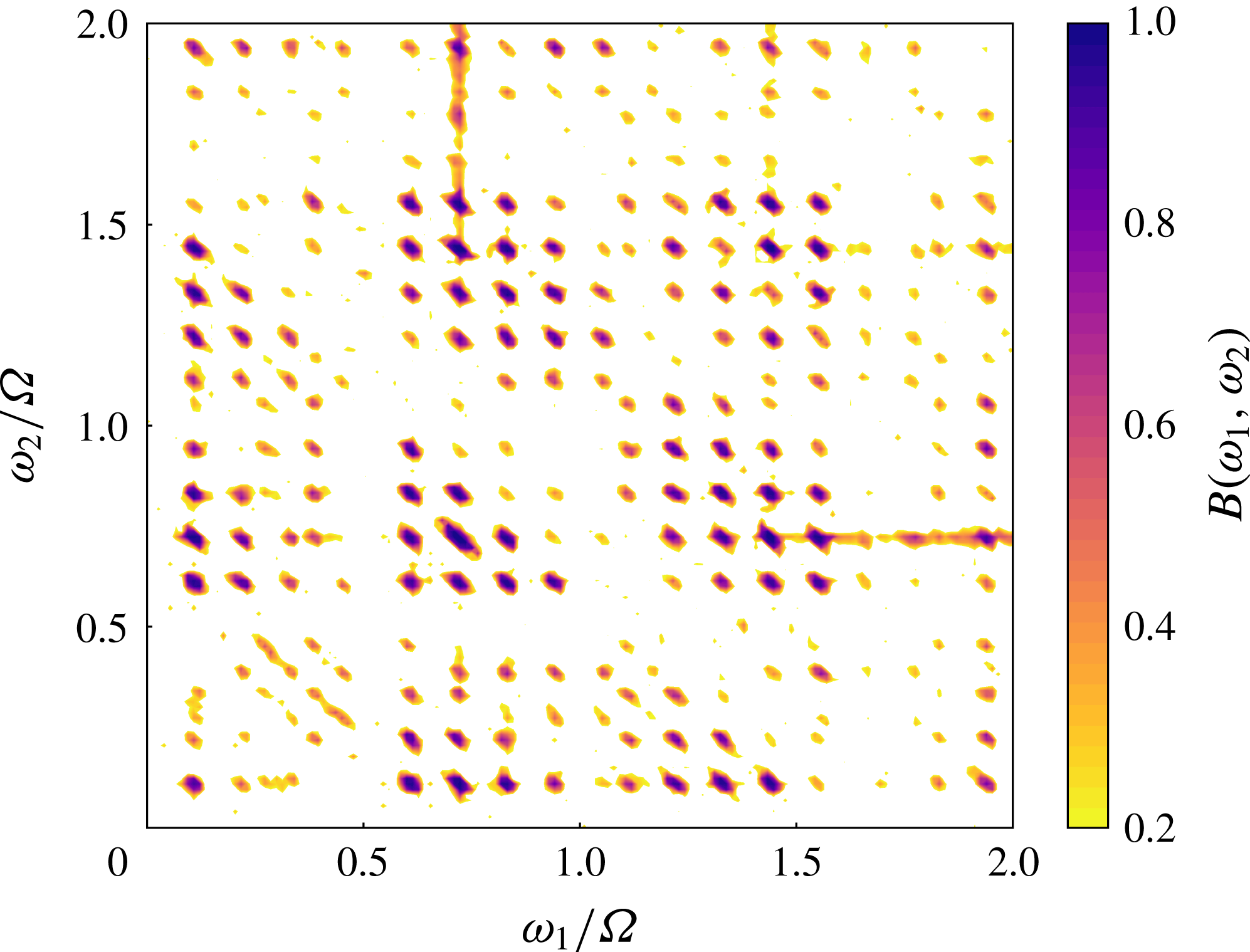
To check that the triads also preserve a consistent phase locking, we compute the bicoherence, defined as
 $$\begin{eqnarray}\displaystyle & \displaystyle B(\unicode[STIX]{x1D714}_{1},\unicode[STIX]{x1D714}_{2})=\frac{\displaystyle \left|\mathop{\sum }_{n}F_{n}(\unicode[STIX]{x1D714}_{1})F_{n}(\unicode[STIX]{x1D714}_{2})F_{n}^{\dagger }(\unicode[STIX]{x1D714}_{1}+\unicode[STIX]{x1D714}_{2})\right|^{2}}{|F_{n}(\unicode[STIX]{x1D714}_{1})F_{n}(\unicode[STIX]{x1D714}_{2})|^{2}|F_{n}(\unicode[STIX]{x1D714}_{1}+\unicode[STIX]{x1D714}_{2})|^{2}}, & \displaystyle\end{eqnarray}$$
where
 $F(\unicode[STIX]{x1D714})$
represents the Fourier transform of a signal at frequency
 $\unicode[STIX]{x1D714}$
and
 $^{\dagger }$
denotes a complex conjugate. This is a statistical measure of the quadratic phase coupling (Nikias & Raghuveer Reference Nikias and Raghuveer1987) determined by splitting a signal into several parts, computing the ‘bispectrum’ (one of the terms in the numerator) of individual parts and eventually summing them up. Wave interactions that preserve the same phase relation over the different parts of the time series result in a particularly strong
 $B(\unicode[STIX]{x1D714}_{1},\unicode[STIX]{x1D714}_{2})$
.
We compute the bicoherence for a time series of zonal velocity,
 $u_{\unicode[STIX]{x1D719}}$
, that we split into 16 segments overlapping by 50 % using the HOSA Matlab toolbox (Swami, Mendel & Nikias Reference Swami, Mendel and Nikias1998). For each segment, 4096 points are used for the fast Fourier transform. The bicoherence
 $B(\unicode[STIX]{x1D714}_{1},\unicode[STIX]{x1D714}_{2})$
attains a high value for all identified triadic resonances, as shown in figure 19. For example, take the peak of
 $(\unicode[STIX]{x1D714}_{1},\unicode[STIX]{x1D714}_{2})=(0.61,0.11)$
representing the coupling for the
 $(4,1)$
mode and
 $m=1$
SI mode seen in this regime. In this case
 $B(0.61,0.11)$
has a very high value, as these modes are phase coupled to the
 $(3,2)$
mode, having a frequency of
 $0.61+0.11=0.72$
. The couplings with higher frequencies denote triadic resonances between pairs of higher harmonics of the
 $(3,2)$
,
 $(4,1)$
and
 $(10,3)$
modes and the higher harmonics of the
 $m=1$
SI mode. Strong self-interactions along the main diagonal can also be seen, especially for the dominant
 $(3,2)$
mode.
Bicoherence of
 $u_{\unicode[STIX]{x1D719}}$
time series taken at
 $r=0.7r_{o}$
, computed for
 $E=10^{-4}$
and
 $\unicode[STIX]{x0394}\unicode[STIX]{x1D6FA}/\unicode[STIX]{x1D6FA}=-2$
. All frequencies are non-dimensionalised by
 $\unicode[STIX]{x1D6FA}$
. Compare with figure 6 from Hoff et al. (Reference Hoff, Harlander and Triana2016b
).

The major modes forming triadic resonances at
 $E=10^{-5}$
and the degree to which they satisfy the frequency criterion are shown in figure 20. The pairs forming triads with the
 $m=1$
SI mode are
 $[(5,2),(6,1)]$
,
 $[(4,3),(5,2)]$
,
 $[(3,2),(6,1)]$
and
 $[(10,3),(3,2)]$
. These triads have also been found in experiments at BTU C-S (Hoff et al.
Reference Hoff, Harlander, Egbers, Triana, Egbers, Ruck, Leder and Dopheide2016a
,Reference Hoff, Harlander and Triana
b
).
Triadic resonances at
 $E=10^{-5}$
. Here
 $\unicode[STIX]{x1D714}_{diff}$
refers to the lines of various frequency differences which form triadic resonances;
 $\unicode[STIX]{x1D714}_{diff}$
is close to zero at all times.

8 Onset of inertial modes
Since pairs of the ‘fast’ inertial EA modes form triadic resonances with the
 $m=1$
SI mode, there are two possible onset scenarios:
(i) The EA modes are secondary instabilities of the ES modes – the
$m=1$
SI and its higher harmonics. This mechanism would be similar to that of the shear and elliptical instabilities of precessing flow (Kerswell Reference Kerswell1993), where a background flow becomes unstable to two inertial modes and the three form a triadic resonance. For the present system, this would mean that the pairs of EA modes are to be interpreted as an instability of the
$m=1$
SI and could only appear together and always at the same time.(ii) The EA modes are instabilities of the background flow. If the background flow (
$m=0$
) becomes unstable, it would give rise to not two but a single EA mode, which would then dominate the solution. The nonlinear interaction of this dominant mode with the
$m=1$
SI mode would excite a third member of the triad.


To determine whether the
 $m=1$
SI mode is essential for the appearance of fast inertial modes, we suppress its onset by restricting the symmetry in numerical experiments. We choose the onset of the EA modes at
 $E=10^{-4}$
as a test case since it is computationally less demanding. We initiate our simulations from an axisymmetric state and add an initial random noise perturbation to all spherical harmonic coefficients. Thereafter, we allow only all axisymmetric
 $m=0$
modes and all EA modes to grow.
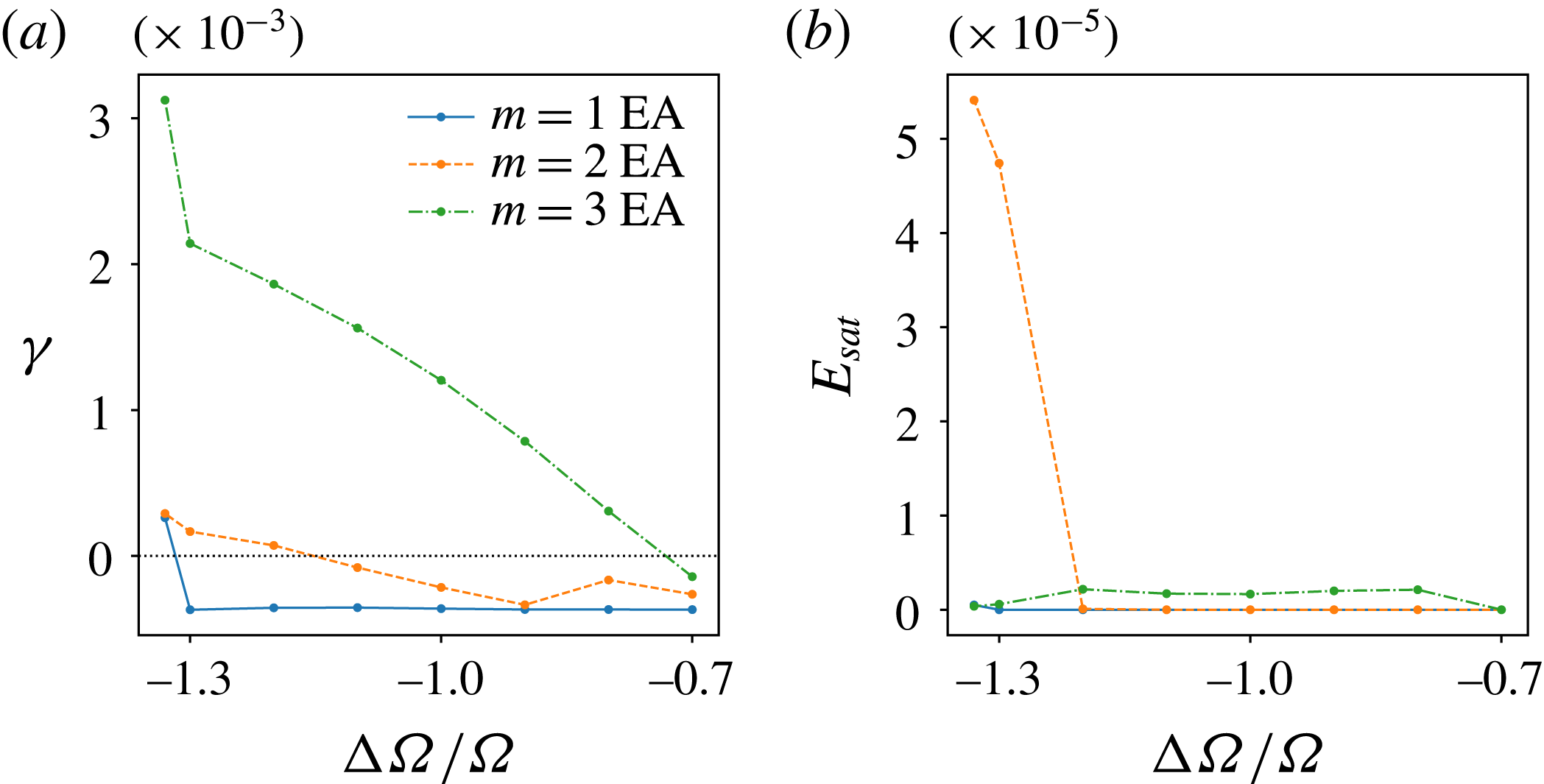
The first instability is the
 $(4,3)$
mode, which sets in at around
 $\unicode[STIX]{x0394}\unicode[STIX]{x1D6FA}/\unicode[STIX]{x1D6FA}=-0.75$
, as shown in figure 21(a). The
 $(3,2)$
mode sets in as a secondary instability at around
 $\unicode[STIX]{x0394}\unicode[STIX]{x1D6FA}/\unicode[STIX]{x1D6FA}=-1.2$
. As figure 21(b) shows, the
 $(4,3)$
mode remains rather weak while the
 $(3,2)$
mode saturates at a much higher energy. Finally, at
 $\unicode[STIX]{x0394}\unicode[STIX]{x1D6FA}/\unicode[STIX]{x1D6FA}=-1.33$
, where the onset of EA modes takes place for the full system, we find the emergence of an
 $m=1$
EA mode, which could not be identified owing to its twisted structure. In the absence of any equatorially symmetric mode, there are no triads in the system.
(a) Growth rates
 $\unicode[STIX]{x1D6FE}$
and (b) saturation energies
 $E_{max}$
of EA modes at different
 $\unicode[STIX]{x0394}\unicode[STIX]{x1D6FA}/\unicode[STIX]{x1D6FA}$
. The horizontal line in (a) marks zero growth rate.

The above observations show that the fast inertial modes are secondary instabilities of the background flow. Even though the equatorially symmetric instabilities of the system are not essential to their onset, they play a key role in the mode selection. For example, the onset of the
 $(4,3)$
instability is suppressed while the critical
 $\unicode[STIX]{x0394}\unicode[STIX]{x1D6FA}/\unicode[STIX]{x1D6FA}$
for the onset of the
 $(3,2)$
mode is slightly shifted as compared to the full system. The resonant triads are not a prerequisite for the appearance of the EA modes but a consequence of the fact that the
 $m=1$
SI mode is already present when these modes set in.
9 Conclusion
The experiments at BTU C-S allowed the spherical Couette system to be explored in a parameter regime also accessible to numerical simulations. We have used the two codes MagIC and XSHELLS for a detailed study at Ekman numbers
 $E=10^{-4}$
and
 $10^{-5}$
and a close comparison to the experiment for the latter parameter. All the principal regimes and modes discovered in the experiment are recovered by the numerics. The complete access to the full solution in the simulations not only confirmed the sometimes challenging mode identifications in the laboratory but also revealed additional instabilities. Projection of the velocity solution onto inertial modes was an additional tool complementing visual characterisation of inertial modes and frequency matching using temporal analyses.
At
 $E=10^{-4}$
, the first instability is a Stewartson layer instability with
 $m=1$
, which shows dominant contributions from the
 $(3,1)$
,
 $(5,1)$
and
 $(7,1)$
modes. We are thus not able to identify it as a single inertial mode and refer to it as the
 $m=1$
SI. For
 $E\leqslant 10^{-5}$
, this mode becomes an important secondary instability, which is, for example, slightly preceded by an
 $m=2$
instability at
 $E=10^{-5}$
. This is followed by a regime characterised by ‘fast’ equatorially antisymmetric (EA) inertial modes.
At
 $E=10^{-4}$
, the
 $(3,2)$
mode dominates while at
 $E=10^{-5}$
the more complex
 $(5,2)$
mode is initially more prominent, most likely due to a smaller viscous dissipation. The EA inertial modes are modified by the presence of the background flow and therefore differ from the respective eigenmodes of a sphere or a spherical shell in frequency and structure. However, the modifications are small enough to still allow a clear identification in most cases. Not surprisingly, their shape is mostly modified at the Stewartson layer and inside the TC where the shear exerted by the background flow is strongest. By artificially exciting the inertial mode
 $(3,2)$
at
 $E=10^{-4}$
at various differential rotation rates, we could trace how its frequency increases from a perfect match with the eigenmode prediction at
 $\unicode[STIX]{x0394}\unicode[STIX]{x1D6FA}/\unicode[STIX]{x1D6FA}=0$
to the value found for the full simulations at
 $\unicode[STIX]{x0394}\unicode[STIX]{x1D6FA}/\unicode[STIX]{x1D6FA}=-1.33$
. Numerical simulations and experiments span four decades in Ekman number but the frequency changes by only about 10 %. We speculate this frequency change goes along with a change in critical differential rotation, which decreases in magnitude with Ekman number.
A striking feature of the EA inertial modes is that they always come in pairs that form resonant triads with the
 $m=1$
SI mode. Triads are found for many wave phenomena and require that the nonlinear interaction between two modes matches the wavenumber, frequency and equatorial symmetry of a third mode and that the three modes are coupled in phase. This was already previously suggested by Hoff et al. (Reference Hoff, Harlander and Triana2016b
); our mode projections substantiate this inference.
To explore whether the triads with the
 $m=1$
SI are essential for facilitating the onset for the EA modes, we conducted numerical experiments where this fundamental mode was suppressed. Since fast inertial modes were still excited and could exist as the only non-axisymmetric instability in the system, we conclude that the triads are mostly a consequence of an EA mode onset and not a condition. Once, for example, the
 $(3,2)$
mode has set in, the triadic resonance with the
 $m=1$
SI immediately feeds energy into the
 $(4,1)$
EA mode. The existence of the triads certainly changes the system behaviour in the sense that the EA mode onset is shifted and that EA modes set in other than the ones preferred for a pure axisymmetric background flow. The resonance more easily allows the system to drain energy from the imposed differential rotation. The system therefore seems to prefer the resonances and manages to maintain them over a larger range of differential rotation.
At
 $E=10^{-5}$
we find a cessation of triads at intermediate differential rotation rates. The background flow and nonlinear interaction may have modified the modes to such an extent that resonance becomes infeasible. However, at a larger
 $|\unicode[STIX]{x0394}\unicode[STIX]{x1D6FA}/\unicode[STIX]{x1D6FA}|$
value, another triad with the
 $m=1$
SI becomes possible and the respective new EA modes set in. A succession of several EA inertial modes has been reported for the 3 m experiment (Triana Reference Triana2011), when
 $\unicode[STIX]{x0394}\unicode[STIX]{x1D6FA}/\unicode[STIX]{x1D6FA}$
is decreased to more negative values. We speculate that this has a similar origin, though the triadic pairs have not been clearly identified for this experiment. For a very high magnitude of differential rotation, however, the
 $(4,1)$
mode clearly dominates the flow without any other strong mode being present. This confirms that triads are not required to support EA modes but are preferred under certain conditions. More exploration is certainly required to clarify this point.
Finally, we note that the critical magnitude of differential rotation needed to excite the fundamental
 $m=1$
SI mode or the EA modes seems to decrease with Ekman number. Further investigations at lower Ekman numbers are necessary to understand the scaling of these regime boundaries. A scaling of
 $E^{1/5}$
for the transition to the turbulent regime has already been found in the experiments by Hoff et al. (Reference Hoff, Harlander and Triana2016b
). Such scaling laws would also allow further insight into the experiments of Triana (Reference Triana2011) as well as into the hydrodynamics of astrophysical objects which are at parameter regimes beyond the reach of numerical investigations.
In the introduction we mentioned some key open questions surrounding the EA inertial modes in a wide-gap spherical Couette system. We have shown that the background flow and the presence of the
 $m=1$
SI mode influences the inertial modes and modifies their influence and structure. Also, triadic resonances with this fundamental mode seem to play an important role in the mode selection. Since ‘fast’ inertial modes are not strongly rotationally restricted due to the Taylor–Proudman theorem, both equatorially symmetric and antisymmetric modes can, in principle, occur. Rieutord et al. (Reference Rieutord, Triana, Zimmerman and Lathrop2012) suggest that a critical shear layer is responsible for the excitation. This could explain the preference for retrograde drifting modes at negative differential rotation where a certain region of the Stewartson layer would co-rotate with the drifting mode. This selection criterion only allows modes to be excited where
 $\unicode[STIX]{x1D714}/m\unicode[STIX]{x0394}\unicode[STIX]{x1D6FA}\leqslant 0.5$
(Wicht Reference Wicht2014). This criterion does not explain why only EA modes are excited because equatorially antisymmetric modes, like equatorially symmetric modes, can drift either way. Viscosity may also play a role in the mode selection process, but the influence may be rather limited, as suggested by the very similar critical
 $\unicode[STIX]{x0394}\unicode[STIX]{x1D6FA}/\unicode[STIX]{x1D6FA}$
for specific modes, which remain very similar over four decades in Ekman number. Fully answering these questions needs further exploration; in particular also of the equatorially symmetric inertial modes and positive differential rotation regime.
Acknowledgements
A.B. would like to thank the IMPRS for Solar System Science for funding him and the North-German Supercomputing Alliance (HLRN), Max Planck Computing and Data Facility (MPCDF) and the Gesellschaft für wissenschaftliche Datenverarbeitung mbH Göttingen (GWDG) for generously letting him use their supercomputing facilities. S.A.T. would like to acknowledge support from the European Research Council (ERC Advanced grant 670874 ROTANUT) and from the infrastructure program EuHIT of the European Commission. M.H. gratefully acknowledges support from the German Research Foundation (DFG grant no. HA 2932/7-1). We thank A. Tilgner whose insight and expertise greatly improved the quality of this work. We gratefully acknowledge A. Mazilu from the Transylvania University of Brasov (Romania) for performing most of the experiments in the frame of a Traineeship ERASMUS+ programme.
Appendix A. Condition for triadic resonances
Consider a fluid velocity field
 $\boldsymbol{u}$
being governed by the Navier–Stokes equation (2.1):
 $$\begin{eqnarray}\displaystyle & \displaystyle \displaystyle \frac{\unicode[STIX]{x2202}\boldsymbol{u}}{\unicode[STIX]{x2202}t}+\boldsymbol{u}\boldsymbol{\cdot }\unicode[STIX]{x1D735}\boldsymbol{u}+2\unicode[STIX]{x1D6FA}_{o}\hat{\boldsymbol{z}}\times \boldsymbol{u}+\unicode[STIX]{x1D735}p/\unicode[STIX]{x1D70C}+\unicode[STIX]{x1D6FB}^{2}\boldsymbol{u}=0. & \displaystyle\end{eqnarray}$$
Using the rotational time scale
 $\unicode[STIX]{x1D6FA}_{o}^{-1}$
as time scale, the shell thickness
 $L$
as length scale, and a characteristic velocity scale
 $U$
as velocity scale (similar to Greenspan Reference Greenspan1968), we obtain the following non-dimensional form of the equation:
 $$\begin{eqnarray}\displaystyle & \displaystyle \displaystyle \frac{\unicode[STIX]{x2202}\boldsymbol{u}}{\unicode[STIX]{x2202}t}+Ro(\boldsymbol{u}\boldsymbol{\cdot }\unicode[STIX]{x1D735}\boldsymbol{u})+2\hat{\boldsymbol{z}}\times \boldsymbol{u}+\unicode[STIX]{x1D735}p+E\unicode[STIX]{x1D6FB}^{2}\boldsymbol{u}=0, & \displaystyle\end{eqnarray}$$
where
 $Ro=(UL)/\unicode[STIX]{x1D6FA}_{o}$
is the Rossby number. Expanding
 $\boldsymbol{u}$
and
 $p$
in terms of
 $Ro$
, we obtain
 $$\begin{eqnarray}\displaystyle & \displaystyle \boldsymbol{u}=\boldsymbol{u}_{0}+Ro\,\boldsymbol{u}_{1}+Ro^{2}\boldsymbol{u}_{2}+\cdots \,,\quad p=p_{0}+Ro\,p_{1}+Ro^{2}p_{2}+\cdots \,. & \displaystyle\end{eqnarray}$$
For low Ekman numbers, one can ignore the dissipation term and we recover the inertial mode equation at zeroth order:
 $$\begin{eqnarray}\displaystyle & \displaystyle \displaystyle \frac{\unicode[STIX]{x2202}\boldsymbol{u}_{0}}{\unicode[STIX]{x2202}t}+2\hat{\boldsymbol{z}}\times \boldsymbol{u}_{0}+\unicode[STIX]{x1D735}p_{0}=0. & \displaystyle\end{eqnarray}$$
Thus,
 $$\begin{eqnarray}\displaystyle & \displaystyle \boldsymbol{u}_{0}=\mathop{\sum }_{j}c_{j}(t)\boldsymbol{Q}_{j}\text{e}^{\text{i}(m_{j}\unicode[STIX]{x1D719}-\unicode[STIX]{x1D714}_{j}t)}+\text{c.c.},\quad p_{0}=\mathop{\sum }_{j}c_{j}(t)\unicode[STIX]{x1D6F7}_{j}\text{e}^{\text{i}(m_{j}\unicode[STIX]{x1D719}-\unicode[STIX]{x1D714}_{j}t)}+\text{c.c.}, & \displaystyle\end{eqnarray}$$
where
 $\boldsymbol{Q}$
and
 $\unicode[STIX]{x1D6F7}$
denote inertial modes. At order 1, we obtain
 $$\begin{eqnarray}\displaystyle & \displaystyle \displaystyle \frac{\unicode[STIX]{x2202}\boldsymbol{u}_{1}}{\unicode[STIX]{x2202}t}+2\hat{\boldsymbol{z}}\times \boldsymbol{u}_{1}+\unicode[STIX]{x1D735}p_{1}=-(\boldsymbol{u}_{0}\boldsymbol{\cdot }\unicode[STIX]{x1D735}\boldsymbol{u}_{0}). & \displaystyle\end{eqnarray}$$
Let us examine the right-hand side. Consider that
 $\boldsymbol{u}_{0}$
has dominant inertial mode contributions from two modes
 $\boldsymbol{Q}_{1}$
and
 $\boldsymbol{Q}_{2}$
. We would get
 $$\begin{eqnarray}\displaystyle \displaystyle \mathbf{u}_{0}\boldsymbol{\cdot }\,\unicode[STIX]{x1D735}\mathbf{u}_{0} & = & \displaystyle (c_{1}\mathbf{Q}_{1}\text{e}^{\text{i}(m_{1}\unicode[STIX]{x1D719}-\unicode[STIX]{x1D714}_{1}t)}+c_{2}\mathbf{Q}_{2}\text{e}^{\text{i}(m_{2}\unicode[STIX]{x1D719}-\unicode[STIX]{x1D714}_{2}t)}+\text{c.c.})\nonumber\\ \displaystyle & & \displaystyle \displaystyle \boldsymbol{\cdot }\,\unicode[STIX]{x1D735}(c_{1}\mathbf{Q}_{1}\text{e}^{\text{i}(m_{1}\unicode[STIX]{x1D719}-\unicode[STIX]{x1D714}_{1}t)}+c_{2}\mathbf{Q}_{2}\text{e}^{\text{i}(m_{2}\unicode[STIX]{x1D719}-\unicode[STIX]{x1D714}_{2}t)}+\text{c.c.})\nonumber\\ \displaystyle & & \displaystyle \displaystyle =c_{1}^{2}\left[\left(\mathbf{Q}_{1}\boldsymbol{\cdot }\,\unicode[STIX]{x1D735}\mathbf{Q}_{1}+{\displaystyle \frac{\text{i}m_{1}}{r\sin \unicode[STIX]{x1D703}}}Q_{1\unicode[STIX]{x1D719}}\mathbf{Q}_{1}\right)\text{e}^{2\text{i}(m_{1}\unicode[STIX]{x1D719}-\unicode[STIX]{x1D714}_{1}t)}+\text{c.c.}\right]\nonumber\\ \displaystyle & & \displaystyle \displaystyle +\,c_{2}^{2}\left[\left(\mathbf{Q}_{2}\boldsymbol{\cdot }\,\unicode[STIX]{x1D735}\mathbf{Q}_{2}+{\displaystyle \frac{\text{i}m_{2}}{r\sin \unicode[STIX]{x1D703}}}Q_{2\unicode[STIX]{x1D719}}\mathbf{Q}_{2}\right)\text{e}^{2\text{i}(m_{2}\unicode[STIX]{x1D719}-\unicode[STIX]{x1D714}_{2}t)}+\text{c.c.}\right]\nonumber\\ \displaystyle & & \displaystyle \displaystyle +\,2c_{1}^{2}\mathbf{Q}_{1}\boldsymbol{\cdot }\unicode[STIX]{x1D735}\mathbf{Q}_{1}+2c_{2}^{2}\mathbf{Q}_{2}\boldsymbol{\cdot }\,\unicode[STIX]{x1D735}\mathbf{Q}_{2}\nonumber\\ \displaystyle & & \displaystyle \displaystyle +\,c_{1}c_{2}\left[\left(\mathbf{Q}_{1}\boldsymbol{\cdot }\,\unicode[STIX]{x1D735}\mathbf{Q}_{2}+\mathbf{Q}_{2}\boldsymbol{\cdot }\,\unicode[STIX]{x1D735}\mathbf{Q}_{1}+{\displaystyle \frac{\text{i}m_{1}}{r\sin \unicode[STIX]{x1D703}}}Q_{2\unicode[STIX]{x1D719}}\mathbf{Q}_{1}+{\displaystyle \frac{\text{i}m_{2}}{r\sin \unicode[STIX]{x1D703}}}Q_{1\unicode[STIX]{x1D719}}\mathbf{Q}_{2}\right)\right.\nonumber\\ \displaystyle & & \displaystyle \displaystyle \quad \times \left.\exp [\text{i}((m_{1}+m_{2})\unicode[STIX]{x1D719}-(\unicode[STIX]{x1D714}_{1}+\unicode[STIX]{x1D714}_{2})t)]+\text{c.c.}\right]\nonumber\\ \displaystyle & & \displaystyle \displaystyle +\,c_{1}c_{2}\left[\left(\mathbf{Q}_{1}\boldsymbol{\cdot }\unicode[STIX]{x1D735}\mathbf{Q}_{2}+\mathbf{Q}_{2}\boldsymbol{\cdot }\,\unicode[STIX]{x1D735}\mathbf{Q}_{1}+{\displaystyle \frac{\text{i}m_{1}}{r\sin \unicode[STIX]{x1D703}}}Q_{2\unicode[STIX]{x1D719}}\mathbf{Q}_{1}-{\displaystyle \frac{\text{i}m_{2}}{r\sin \unicode[STIX]{x1D703}}}Q_{1\unicode[STIX]{x1D719}}\mathbf{Q}_{2}\right)\right.\nonumber\\ \displaystyle & & \displaystyle \displaystyle \quad \times \left.\exp [\text{i}((m_{1}-m_{2})\unicode[STIX]{x1D719}-(\unicode[STIX]{x1D714}_{1}-\unicode[STIX]{x1D714}_{2})t)]+\text{c.c.}\right],\end{eqnarray}$$
Let us project
 $\boldsymbol{u}_{1}$
and
 $p_{1}$
from (A 6) onto the inertial mode basis,
 $$\begin{eqnarray}\displaystyle & \displaystyle \boldsymbol{u}_{1}=\mathop{\sum }_{j}a_{j}(t)\boldsymbol{Q}_{j}\text{e}^{\text{i}(m_{j}\unicode[STIX]{x1D719}-\unicode[STIX]{x1D714}_{j}t)}+\text{c.c.},\quad p_{2}=\mathop{\sum }_{j}a_{j}(t)\unicode[STIX]{x1D6F7}_{j}\text{e}^{\text{i}(m_{j}\unicode[STIX]{x1D719}-\unicode[STIX]{x1D714}_{j}t)}+\text{c.c.} & \displaystyle\end{eqnarray}$$
Substituting this in (A 6), we get
 $$\begin{eqnarray}\displaystyle & \displaystyle \mathop{\sum }_{j}\left(\boldsymbol{Q}_{j}{\displaystyle \frac{\text{d}}{\text{d}t}}a_{j}+a_{j}(-\text{i}\unicode[STIX]{x1D714}_{j}\boldsymbol{Q}_{j}+2\hat{\boldsymbol{z}}\times \boldsymbol{Q}_{j}+\unicode[STIX]{x1D735}\unicode[STIX]{x1D6F7}_{j})\right)\text{e}^{\text{i}(m_{j}\unicode[STIX]{x1D719}-\unicode[STIX]{x1D714}_{j}t)}+\text{c.c.}=-(\boldsymbol{u}_{0}\boldsymbol{\cdot }\unicode[STIX]{x1D735}\boldsymbol{u}_{0}).\qquad & \displaystyle\end{eqnarray}$$
By definition,
 $-\text{i}\unicode[STIX]{x1D714}_{j}\boldsymbol{Q}_{j}+2\hat{\boldsymbol{z}}\times \boldsymbol{Q}_{j}+\unicode[STIX]{x1D735}\unicode[STIX]{x1D6F7}_{j}=0$
for all
 $j$
. Thus, we are left with
 $$\begin{eqnarray}\displaystyle & \displaystyle \mathop{\sum }_{j}{\displaystyle \frac{\text{d}}{\text{d}t}}a_{j}(\boldsymbol{Q}_{j}\text{e}^{\text{i}(m_{j}\unicode[STIX]{x1D719}-\unicode[STIX]{x1D714}_{j}t)})+{\displaystyle \frac{\text{d}}{\text{d}t}}a_{j}^{\dagger }(\boldsymbol{Q}_{j}^{\dagger }\text{e}^{\text{i}(-m_{j}\unicode[STIX]{x1D719}+\unicode[STIX]{x1D714}_{j}t)})=-(\boldsymbol{u}_{0}\boldsymbol{\cdot }\unicode[STIX]{x1D735}\boldsymbol{u}_{0}). & \displaystyle\end{eqnarray}$$
Now, we substitute the expression (A 7) that we found for the nonlinear term and project both sides onto a single mode
 $\boldsymbol{Q}_{k}$
:
 $$\begin{eqnarray}\displaystyle \displaystyle -{\displaystyle \frac{\text{d}}{\text{d}t}}a_{k} & = & \displaystyle c_{1}^{2}\int _{0}^{2\unicode[STIX]{x1D70B}}\text{e}^{\text{i}(-m_{k}\unicode[STIX]{x1D719}+\unicode[STIX]{x1D714}_{k}t)}\cos (2(m_{1}\unicode[STIX]{x1D719}-\unicode[STIX]{x1D714}_{1}t))\,\text{d}\unicode[STIX]{x1D719}\int \left(\mathbf{Q}_{1}\boldsymbol{\cdot }\unicode[STIX]{x1D735}\mathbf{Q}_{1}\right)\boldsymbol{\cdot }\mathbf{Q}_{k}^{\dagger }\,\text{d}\unicode[STIX]{x1D70F}\nonumber\\ \displaystyle & & \displaystyle \displaystyle +\,c_{2}^{2}\int _{0}^{2\unicode[STIX]{x1D70B}}\text{e}^{\text{i}(-m_{k}\unicode[STIX]{x1D719}+\unicode[STIX]{x1D714}_{k}t)}\cos (2(m_{2}\unicode[STIX]{x1D719}-\unicode[STIX]{x1D714}_{2}t))\,\text{d}\unicode[STIX]{x1D719}\int \left(\mathbf{Q}_{2}\boldsymbol{\cdot }\unicode[STIX]{x1D735}\mathbf{Q}_{2}\right)\boldsymbol{\cdot }\mathbf{Q}_{k}^{\dagger }\,\text{d}\unicode[STIX]{x1D70F}\nonumber\\ \displaystyle & & \displaystyle \displaystyle +\,2\int _{0}^{2\unicode[STIX]{x1D70B}}\text{e}^{\text{i}(-m_{k}\unicode[STIX]{x1D719}+\unicode[STIX]{x1D714}_{k}t)}\,\text{d}\unicode[STIX]{x1D719}\int \left(c_{1}^{2}\mathbf{Q}_{1}\boldsymbol{\cdot }\unicode[STIX]{x1D735}\mathbf{Q}_{1}+c_{2}^{2}\mathbf{Q}_{2}\boldsymbol{\cdot }\unicode[STIX]{x1D735}\mathbf{Q}_{2}\right)\boldsymbol{\cdot }\mathbf{Q}_{k}^{\dagger }\,\text{d}\unicode[STIX]{x1D70F}\nonumber\\ \displaystyle & & \displaystyle \displaystyle +\,c_{1}c_{2}\int _{0}^{2\unicode[STIX]{x1D70B}}\text{e}^{\text{i}(-m_{k}\unicode[STIX]{x1D719}+\unicode[STIX]{x1D714}_{k}t)}\left[\cos ((m_{1}+m_{2})\unicode[STIX]{x1D719}-(\unicode[STIX]{x1D714}_{1}+\unicode[STIX]{x1D714}_{2})t)\right.\nonumber\\ \displaystyle & & \displaystyle \displaystyle \left.+\,\cos \left((m_{1}-m_{2})\unicode[STIX]{x1D719}-(\unicode[STIX]{x1D714}_{1}-\unicode[STIX]{x1D714}_{2})t\right)\right]\,\text{d}\unicode[STIX]{x1D719}\nonumber\\ \displaystyle & & \displaystyle \displaystyle \quad \times \int \left(\mathbf{Q}_{1}\boldsymbol{\cdot }\unicode[STIX]{x1D735}\mathbf{Q}_{2}+\mathbf{Q}_{2}\boldsymbol{\cdot }\unicode[STIX]{x1D735}\mathbf{Q}_{1}\right)\boldsymbol{\cdot }\mathbf{Q}_{k}^{\dagger }\,\text{d}\unicode[STIX]{x1D70F}\nonumber\\ \displaystyle & = & \displaystyle \displaystyle T_{1}+T_{2}+T_{3}+T_{4},\end{eqnarray}$$
where
 $\text{d}\unicode[STIX]{x1D70F}=r^{2}\sin \unicode[STIX]{x1D703}\,\text{d}r\,\text{d}\unicode[STIX]{x1D703}$
. In the case of each of the terms, for the
 $\unicode[STIX]{x1D719}$
integral to be non-zero and for a resonant excitation, the factors in front of
 $\unicode[STIX]{x1D719}$
and
 $t$
in the exponentials must vanish. This would lead to the following conditions from the different terms:
(i)
$T_{1}$
and
$T_{2}~\Rightarrow ~m_{k}=2m_{1}$
or
$2m_{2}$
and
$\unicode[STIX]{x1D714}_{k}=2\unicode[STIX]{x1D714}_{1}$
or
$2\unicode[STIX]{x1D714}_{2}$
. This is the case when the mode being excited is just a higher harmonic of the existing modes.(ii)
$T_{3}~\Rightarrow ~m_{k}=0$
and
$\unicode[STIX]{x1D714}_{k}=0$
. This is the case of self-interactions giving rise to a geostrophic mode (as already shown by Tilgner Reference Tilgner2007).(iii)
$T_{4}~\Rightarrow ~m_{k}=m_{1}\pm m_{2}$
and
$\unicode[STIX]{x1D714}_{k}=\unicode[STIX]{x1D714}_{1}\pm \unicode[STIX]{x1D714}_{2}$
. This is the case of a triadic resonance of the three modes
$\boldsymbol{Q}_{1}$
,
$\boldsymbol{Q}_{2}$
and
$\boldsymbol{Q}_{k}$
.