











1 Introduction
Hardy space theory takes on many forms and appears in many aspects of mathematics such as harmonic analysis, PDE’s, functional analysis, probability theory, and many others. Interpolation spaces between Hardy spaces in various contexts have a long history. We refer to the articles [Reference Fefferman and Stein13, Reference Jones23, Reference Pisier35] for some background on interpolations between classical Hardy spaces from harmonic analysis and [Reference Janson and Jones18, Reference Weisz47] for interpolations between Hardy spaces from martingale theory. On the other hand, the theory of noncommutative martingales has seen rapid development in many directions. Indeed, since the establishment of the noncommutative Burkholder–Gundy inequalities in [Reference Pisier and Xu37], many classical inequalities are now understood for this context. We refer to the book [Reference Pisier36, Chapter 14] for a summary of some of the main inequalities from noncommutative martingale theory. Further references relevant to our purpose are [Reference Bekjan, Chen, Perrin and Yin1, Reference Chen, Randrianantoanina and Xu7, Reference Junge24, Reference Junge and Xu26, Reference Musat32, Reference Randrianantoanina, Wu and Zhou44]. The main focus of the present article is on Hardy spaces arising from noncommutative martingale theory. More specifically, column/row Hardy spaces defined from column/row conditioned square functions initiated by Junge and Xu in [Reference Junge and Xu26] in connection with the noncommutative Burkholder/Rosenthal inequalities. These spaces are generally referred to as conditioned Hardy spaces and its column (resp. row) version is usually denoted by
 $\mathsf {h}_p^c$
(resp.
 $\mathsf {h}_p^r$
). We would like to emphasize that this particular class of martingale Hardy spaces is instrumental in classical theory. We refer to the monograph [Reference Weisz47] for more in depth treatment of the classical setting. Likewise, the Hardy spaces
 $\mathsf {h}_p^c$
and
 $\mathsf {h}_p^r$
are proven to be fundamental objects in various aspects of the new progress made in the noncommutative martingale theory during the last several years. For instance, the formulation of the noncommutative Burkholder inequality for the case
 $1<p<2$
was mainly due to a reformulation of the case
 $2\leq p<\infty $
as equivalence of norms involving the spaces
 $\mathsf {h}_p^c$
and
 $\mathsf {h}_p^r$
. The asymmetric Doob maximal inequalities in [Reference Hong, Junge and Parcet17] were derived from properties of
 $\mathsf {h}_p^c$
and
 $\mathsf {h}_p^r$
where
 $1\leq p<2$
. The general theme of the present article is on interpolation spaces for the quasi-Banach space couple
 $(\mathsf {h}_p^c, \mathsf {h}_q^c)$
when
 $0<p<q<\infty $
.
To motivate our consideration, let us review some interpolation results from classical martingale theory. Let
 $(\Omega , \mathcal {F},\mathbb {P})$
be a probability space and
 $(\mathcal {F}_n)_{n\geq 1}$
be an increasing sequence of
 $\sigma $
-subfields of
 $\mathcal {F}$
satisfying the condition
 $\mathcal {F}=\sigma (\bigcup _{n\geq 1} \mathcal {F}_n)$
. For
 $0<p \leq \infty $
, denote by
 $\mathcal {H}_p(\Omega )$
(resp.
 $\mathsf {h}_p(\Omega )$
) the martingale Hardy space defined by square functions (resp. conditioned square functions) and
 ${\mathcal {BMO}}(\Omega )$
(resp.
 $\mathsf {bmo}(\Omega )$
) the martingale BMO (resp. martingale little BMO) space associated with the filtration
 $(\mathcal {F}_n)_{n\geq 1}$
. We refer to [Reference Garsia14, Reference Weisz47] for precise definitions and properties of these spaces along with discussions on their importance for the classical theory. It is well established in the literature that the spaces
 ${\mathcal {BMO}}(\Omega )$
and
 $\mathsf {bmo}(\Omega )$
play important role in interpolation theory as they may be used as natural substitutes for
 $L_\infty (\Omega )$
. Our motivation comes from the following three classical results that involved martingale BMO spaces as one of the endpoints of interpolations:
 $$ \begin{align} \big[\mathcal{H}_1(\Omega) , {\mathcal {BMO}}(\Omega)\big]_{\theta} = \mathcal{H}_r(\Omega), \quad 0<\theta<1 \ \text{and}\ \frac{1}{r}= 1-\theta; \end{align} $$
 $$ \begin{align} \big[\mathcal{H}_p(\Omega) , {\mathcal {BMO}}(\Omega) \big]_{\theta} \subsetneq \mathcal{H}_r(\Omega), \quad 0<p<1,\ 0<\theta<1,\ \text{and} \ \frac{1}{r}= \frac{1-\theta}{p}<1; \end{align} $$
 $$ \begin{align} \big(\mathsf{h}_p(\Omega) , \mathsf{bmo}(\Omega) \big)_{\theta, r} = \mathsf{h}_r(\Omega), \quad 0<p<\infty, \ 0<\theta<1, \ \text{and}\ \frac{1}{r}= \frac{1-\theta}{p}, \end{align} $$
where
 $[\cdot ,\cdot ]_\theta $
(resp.
 $(\cdot ,\cdot )_{\theta , r}$
) denotes the complex (resp. real) interpolation method. The identity (1.1) and the inclusion (1.2) were obtained by Janson and Jones in [Reference Janson and Jones18], whereas (1.3) was established in its present form by Weisz in [Reference Weisz46]. It is a natural question to consider if the three assertions stated above still hold for the noncommutative setting. The first result in this direction is due to Musat in [Reference Musat32] who proved a noncommutative analogue of (1.1) where as introduced in [Reference Pisier and Xu37], the noncommutative Hardy space
 $\mathcal {H}_1$
is the sum of the column version and the row version and the BMO space is defined as the intersection of column BMO and the row BMO. Later, Bekjan et al. established in [Reference Bekjan, Chen, Perrin and Yin1] that the noncommutative analogue of (1.3) holds for the Banach space range. That is, (1.3) remains valid for the interpolation couple
 $(\mathsf {h}_1^c, \mathsf {bmo}^c)$
. To the best of our knowledge, [Reference Bekjan, Chen, Perrin and Yin1] and [Reference Musat32] are the only articles available in the literature that contain substantial advances in the study of interpolation spaces of noncommutative martingale Hardy spaces to date. The present paper extends the interpolation results from [Reference Bekjan, Chen, Perrin and Yin1] to the case
 $0<p<1$
thus providing a full noncommutative generalization of (1.3) for column/row spaces. We refer to Theorem 3.5 for detailed formulation. We also obtained interpolation spaces between spaces of adapted sequences which may be viewed as the right substitute for (1.1) when
 $0<p<1$
. This is stated in Theorem 3.13. We should point out that the result on the spaces of adapted sequences appears to be new even for the classical setting. Moreover, the noncommutative analogue of (1.2) can be easily deduced from the result on adapted sequences.
Our method of proof is very different from [Reference Bekjan, Chen, Perrin and Yin1, Reference Musat32]. In fact, the techniques used in both [Reference Bekjan, Chen, Perrin and Yin1] and [Reference Musat32] appear to work only for Banach couples. Our main objective is to compare K-functionals for the couple
 $(\mathsf {h}_p^c, \mathsf {h}_q^c)$
where
 $0<p<q<\infty $
to those associated to the well-known couple
 $(L_p, L_q)$
associated with appropriate amplified von Neumann algebras. In the classical setting, this type of reduction is usually achieved through some strategic use of stopped martingales. We note that a the time of this writing there is no direct analogue of stopping times available for the noncommutative setting but the so-called Cuculescu projections [Reference Cuculescu8] are often used as a substitute for stopping times. However, Cuculescu projections do not appear to be efficient enough to provide the desired truncations. This makes our approach very different from the classical setting as found in [Reference Janson and Jones18, Reference Weisz46]. Our method is based on the so-called algebraic atomic decompositions. The notion of algebraic atoms were introduced by Perrin in [Reference Perrin34] for Junge’s noncommutative conditioned
 $L_p$
spaces and the Hardy spaces
 $\mathsf {h}_p^c$
for
 $1\leq p<2$
and found to be instrumental in the study of Doob’s maximal inequality for martingale in noncommutative Hardy spaces [Reference Hong, Junge and Parcet17]. Algebraic atomic decompositions for the Hardy space
 $\mathsf {h}_p^c$
with
 $0<p<1$
was recently studied in [Reference Chen, Randrianantoanina and Xu7] by constructive approach. Another recent development in this direction is that the noncommutative Orlicz–Hardy space
 $\mathsf {h}_\Phi ^c$
admits algebraic atomic decomposition for convex function
 $\Phi $
satisfying some natural conditions. Using insights from the constructive approach used in [Reference Chen, Randrianantoanina and Xu7, Reference Randrianantoanina, Wu and Zhou44], we established that noncommutative conditioned Orlicz–Hardy spaces admit version of algebraic atomic decompositions when the Orlicz function is p-convex and q-concave for
 $0<p<q<2$
(see Theorem 2.8 for details). These more general atomic decompositions turn out to be one of the decisive tools we used for our results on K-functionals for the couple
 $(\mathsf {h}_p^c, \mathsf {h}_q^c)$
when the distance between p and q is sufficiently small. The results on K-functionals coupled with the well-known Wolff’s interpolation theorem provide the full noncommutative generalization of (1.3). The case of spaces of adapted sequences is handle with the same techniques. That is, estimating the K-functionals through some version of algebraic atomic decompositions.
The paper is organized as follows. In the next section, we review the basics of noncommutative symmetric quasi-Banach spaces following the formulation of [Reference Kalton and Sukochev28, Reference Xu50] and give full detailed accounts of the construction of noncommutative martingale conditioned Hardy spaces associated with symmetric quasi-Banach spaces. We also formulate and prove the algebraic decomposition for noncommutative conditioned spaces associated with Orlicz function spaces and for spaces of adapted sequences.
Section 3 contains formulations and proofs of our principal results: noncommutative generalization of (1.2), noncommutative generalization of (1.3), and an extension of (1.1) to the full range when spaces of adapted sequences are used.
In Section 4, we explore some further applications of our results and methods from Sections 2 and 3 to various inequalities involving noncommutative martingale Hardy spaces in the context of general symmetric spaces of measurable operators.
2 Definitions and preliminary results
Throughout, we adopt the notation
 $A\lesssim _\alpha B$
to indicate that there is a constant
 $C_\alpha $
depending only on the parameter
 $\alpha $
such that the inequality
 $A \leq C_\alpha B$
is satisfied. Similarly,
 $A\approx _\alpha B$
is used if both
 $A\lesssim _\alpha B$
and
 $B \lesssim _\alpha A$
hold.
2.1 Noncommutative symmetric spaces
Throughout,
 $\mathcal {M}$
denotes a semifinite von Neumann algebra equipped with a faithful normal semifinite trace
 $\tau $
. Let
 $\widetilde {\mathcal {M}}$
denote the associated topological
 $*$
-algebra of
 $\tau $
-measurable operators in the sense of [Reference Fack and Kosaki12]. For
 $x \in \widetilde {\mathcal {M}}$
, we recall that its generalized singular number
 $\mu (x)$
is the real-valued function defined by
 $$ \begin{align*} \mu_t(x)= \inf\big\{ s>0 : \tau\big(\chi_{(s,\infty)}(|x|)\big)\leq t\big\}, \quad t>0, \end{align*} $$
where
 $\chi _{(s,\infty )}(|x|)$
is the spectral projection of
 $|x|$
associated with the interval
 $(s,\infty )$
. We observe that if
 $\mathcal {M}$
is the abelian von Neumann algebra
 $L_\infty (0,\infty )$
with the trace given by integration with respect to the Lebesgue measure, then
 $\widetilde {\mathcal {M}}$
becomes the space of measurable complex functions on
 $(0,\infty )$
which are bounded except on a set of finite measure and for
 $f\in \widetilde {\mathcal {M}}$
,
 $\mu (f)$
is precisely the usual decreasing rearrangement of the function
 $|f|$
. We refer to [Reference Pisier and Xu38] for more information on noncommutative integration.
We denote by
 $L_0$
, the space of measurable functions on the interval
 $(0,\infty )$
. Recall that a quasi-Banach function space
 $(E,\|\cdot \|_E)$
of measurable functions on the interval
 $(0,\infty )$
is called symmetric if for any
 $g \in E$
and any
 $f \in L_0$
with
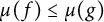 $\mu (f) \leq \mu (g)$
, we have
 $f \in E$
and
 $\|f\|_E \leq \|g\|_E$
. Throughout, all function spaces are assumed to be defined on the interval
 $(0,\infty )$
.
Let E be a symmetric quasi-Banach function space. We define the corresponding noncommutative space by setting:
 $$ \begin{align*} E(\mathcal{M}, \tau) = \big\{ x \in \widetilde{\mathcal{M}}\ : \ \mu(x) \in E \big\}. \end{align*} $$
Equipped with the quasi-norm
 $\|x\|_{E(\mathcal {M},\tau )} := \| \mu (x)\|_E$
, the linear space
 $E(\mathcal {M},\tau )$
becomes a complex quasi-Banach space [Reference Kalton and Sukochev28, Reference Xu50] and is usually referred to as the noncommutative symmetric space associated with
 $(\mathcal {M},\tau )$
corresponding to E. We remark that if
 $0< p<\infty $
and
 $E=L_p$
, then
 $E(\mathcal {M}, \tau )$
is exactly the usual noncommutative
 $L_p$
-space
 $L_p(\mathcal {M},\tau )$
associated with
 $(\mathcal {M},\tau )$
. In the sequel,
 $E(\mathcal {M},\tau )$
will be abbreviated to
 $E(\mathcal {M})$
.
Other classes of examples that are relevant for our purpose are the class of Orlicz spaces and the class of Lorentz spaces. We review these two classes for convenience.
A function
 $\Phi : [0,\infty ) \to [0,\infty )$
is called an Orlicz function whenever it is strictly increasing, continuous,
 $\Phi (0)=0$
, and
 $\lim _{u\to \infty }\Phi (u)=\infty $
. The Orlicz space
 $L_\Phi $
is the collection of all
 $f\in L_0$
for which there exists a constant c such that
 $I_\Phi (|f|/c)<\infty $
where the modular functional
 $I_\Phi (\cdot )$
is defined by:
 $$ \begin{align*} I_\Phi(|g|)=\int_0^\infty \Phi(|g(t)|)\ dt, \quad g \in L_0. \end{align*} $$
The space
 $L_\Phi $
is equipped with the Luxemburg quasi-norm:
 $$ \begin{align*} \big\|f \big\|_{L_\Phi}= \inf\big\{ c>0 : I_\Phi(|f|/c) \leq 1\big\}. \end{align*} $$
If
 $\Phi $
is convex then
 $L_\Phi $
is a symmetric Banach function space. However, we do not restrict ourselves to just the case of normed spaces. We refer to [Reference Turpin45] for Orlicz spaces associated with non necessarily convex functions.
We recall that for
 $0<p \leq q<\infty $
,
 $\Phi $
is called p-convex (resp., q-concave) if the function
 $t\mapsto \Phi (t^{1/p})$
(resp.,
 $t\mapsto \Phi (t^{1/q})$
) is convex (resp., concave). Below, we only consider Orlicz spaces associated with Orlicz functions that are p-convex and q-concave for some
 $0<p\leq q<2$
.
For the next relevant example, assume that
 $0<p,q\leq \infty $
. The Lorentz space
 $L_{p,q}$
is the space of all
 $f \in L_0$
for which
 $\|f\|_{p,q}<\infty $
where
 $$ \begin{align*} \big\|f \big\|_{p,q} =\begin{cases} \left(\displaystyle{\int_{0}^\infty \mu_{t}^{q}(f)\ d(t^{q/p})}\right)^{1/q}, &0< q < \infty; \\ \displaystyle{\mathop{\mathrm{sup}}_{t>0} t^{1/p} \mu_t(f)}, &q= \infty. \end{cases} \end{align*} $$
If
 $1\leq q\leq p <\infty $
or
 $p=q=\infty $
, then
 $L_{p,q}$
is a symmetric Banach function space. If
 $1<p<\infty $
and
 $p\leq q\leq \infty $
, then
 $L_{p,q}$
can be equivalently renormed to become a symmetric Banach function [Reference Bennett and Sharpley2, Theorem 4.6]. In general,
 $L_{p,q}$
is only a symmetric quasi-Banach function space.
Both noncommutative Orlicz spaces and noncommutative Lorentz spaces will be heavily involved throughout the paper.
2.2 Martingale Hardy spaces and conditioned spaces
In the sequel, we always denote by
 $(\mathcal {M}_n)_{n \geq 1}$
an increasing sequence of von Neumann subalgebras of
 ${\mathcal {M}}$
whose union is w*-dense in
 $\mathcal {M}$
. For every
 $n\geq 1$
, we assume that there is a trace preserving conditional expectation
 $\mathcal {E}_n$
from
 ${\mathcal {M}}$
onto
 ${\mathcal {M}}_n$
.
Definition 2.1 A sequence
 $x = (x_n)_{n\geq 1}$
in
 $L_1(\mathcal {M})+\mathcal {M}$
is called a noncommutative martingale with respect to
 $({\mathcal {M}}_n)_{n \geq 1}$
if
 $\mathcal {E}_n (x_{n+1}) = x_n$
for every
 $n \geq 1$
.
Let E be a symmetric quasi-Banach function space and
 $x=(x_n)_{n\geq 1}$
be a martingale. If for every
 $n\geq 1$
,
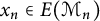 $x_n \in E(\mathcal {M}_n)$
, then we say that
 $(x_n)_{n\geq 1}$
is an
 $E(\mathcal {M})$
-martingale. In this case, we set
 $$ \begin{align*}\| x \|_{E(\mathcal{M})}= \mathop{\mathrm{sup}}_{n \geq 1} \| x_n \|_{E(\mathcal{M})}. \end{align*} $$
If
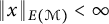 $\| x \|_{E(\mathcal {M})} < \infty $
, then x will be called a bounded
 $E(\mathcal {M})$
-martingale.
For a martingale
 $x=(x_n)_{n\geq 1}$
, we set
 $dx_n=x_n-x_{n-1}$
for
 $n\geq 1$
with the usual convention that
 $x_0=0$
. The sequence
 $dx=(dx_n)_{n\geq 1}$
is called the martingale difference sequence of x. A martingale x is called a finite martingale if there exists N such that
 $dx_n=0$
for all
 $n\geq N$
.
Let us now review some basic definitions related to martingale Hardy spaces associated to noncommutative symmetric spaces.
Following [Reference Pisier and Xu37], we define the column square functions of a given martingale
 $x = (x_k)$
by setting:
 $$ \begin{align*} S_{c,n} (x) = \left ( \sum^n_{k = 1} |dx_k |^2 \right )^{1/2}, \quad S_c (x) = \left ( \sum^{\infty}_{k = 1} |dx_k |^2 \right )^{1/2}. \end{align*} $$
The conditioned versions were introduced in [Reference Junge and Xu26]. For a given
 $L_2(\mathcal {M}) +\mathcal {M}$
-martingale
 $(x_k)_{k\geq 1}$
, we set
 $$ \begin{align*} s_{c,n} (x) = \left ( \sum^n_{k = 1} \mathcal{E}_{k-1}|dx_k |^2 \right )^{1/2}, \quad s_c (x) = \left ( \sum^{\infty}_{k = 1} \mathcal{E}_{k-1}|dx_k |^2 \right )^{1/2}. \end{align*} $$
The operator
 $s_c(x)$
is called the column conditioned square function of x. For convenience, we will use the notation
 $$ \begin{align*} \mathcal{S}_{c,n}(a)= \left ( \sum^n_{k = 1} |a_k |^2 \right )^{1/2}, \quad \mathcal{S}_c (a) = \left ( \sum^{\infty}_{k = 1} |a_k |^2 \right )^{1/2}\, \end{align*} $$
and
 $$ \begin{align*} \sigma_{c,n} (b) = \left ( \sum^{n}_{k = 1} \mathcal{E}_{k-1}|b_k |^2 \right )^{1/2}, \quad \sigma_c (b) = \left ( \sum^{\infty}_{k = 1} \mathcal{E}_{k-1}|b_k |^2 \right )^{1/2} \end{align*} $$
for sequences
 $a=(a_k)_{k\geq 1}$
in
 $L_1(\mathcal {M})+\mathcal {M}$
and
 $b=(b_k)_{k\geq 1}$
in
 $L_2(\mathcal {M}) +\mathcal {M}$
that are not necessarily martingale difference sequences. It is worth pointing out that the infinite sums of positive operators stated above may not always make sense as operators, but we only consider below the special cases where they do converge in the sense of the measure topology.
We will now describe various noncommutative martingale Hardy spaces associated with symmetric quasi-Banach function spaces.
Assume that E is a symmetric quasi-Banach function space. We denote by
 $\mathcal {F}_E$
the collection of all finite martingales in
 $E(\mathcal {M})$
. For
 $x=(x_k)_{k\geq 1} \in \mathcal {F}_E$
, we set:
 $$ \begin{align*} \| x \|_{\mathcal{H}_E^c}= \| S_c(x)\|_{E(\mathcal{M})}. \end{align*} $$
Then
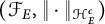 $(\mathcal {F}_E, \|\cdot \|_{\mathcal {H}_E^c})$
is a quasi-normed space. If we denote by
 $(e_{i,j})_{i,j \geq 1}$
the family of unit matrices in
 $B(\ell _2(\mathbb {N}))$
, then the correspondence
 $x\mapsto \sum _{k\geq 1} dx_k \otimes e_{k,1}$
maps
 $\mathcal {F}_E$
isometrically into a (not necessarily closed) linear subspace of
 $E(\mathcal {M}\overline {\otimes } B(\ell _2(\mathbb {N})))$
. We define the column Hardy space
 $\mathcal {H}_E^c (\mathcal {M})$
to be the completion of
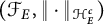 $(\mathcal {F}_E, \|\cdot \|_{\mathcal {H}_E^c})$
. It then follows that
 $\mathcal {H}_E^c(\mathcal {M})$
embeds isometrically into a closed subspace of the quasi-Banach space
 $E(\mathcal {M}\overline {\otimes } B(\ell _2(\mathbb {N})))$
.
In the sequel, we will also make use of the more general space
 $E(\mathcal {M};\ell _2^c)$
which is defined as the set of all sequences
 $a=(a_k)$
in
 $E(\mathcal {M})$
for which
 $\mathcal {S}_c(a) \in E(\mathcal {M})$
. In this case, we set
 $$ \begin{align*} \big\|a \big\|_{E(\mathcal{M};\ell_2^c)} = \|\mathcal{S}_c(a) \|_{E(\mathcal{M})}. \end{align*} $$
Under the above quasi-norm, one can easily see that
 $E(\mathcal {M};\ell _2^c)$
is a quasi-Banach space. The closed subspace of
 $E(\mathcal {M};\ell _2^c)$
consisting of adapted sequences will be denoted by
 $E^{\text {ad}}(\mathcal {M};\ell _2^c)$
. That is,
 $$ \begin{align*} E^{\text{ad}}(\mathcal{M};\ell_2^c)=\big\{ (a_n)_{n\geq 1} \in E(\mathcal{M};\ell_2^c) : \forall n\geq 1, a_n \in E(\mathcal{M}_n) \big\}. \end{align*} $$
Note that for
 $1<p<\infty $
, it follows from the noncommutative Stein inequality that
 $L_p^{\text {ad}}(\mathcal {M};\ell _2^c)$
is a complemented subspace of
 $L_p(\mathcal {M};\ell _2^c)$
. One should not expect such complementation if one merely assume that E is a quasi-Banach symmetric function space.
Next, we will discuss conditioned versions of the spaces defined earlier. Consider the linear space
 $\mathcal {FS}$
consisting of all
 $x \in \mathcal {M}$
such that there exists a projection
 $e\in \mathcal {M}_1$
,
 $\tau (e)<\infty $
, and
 $x=exe$
. We should note that if
 $\mathcal {M}$
is finite, then
 $\mathcal {FS}=\mathcal {M}$
. For every
 $n\geq 1$
and
 $0<p \leq \infty $
, we define the space
 $L_p^c(\mathcal {M},\mathcal {E}_n)$
to be the completion of
 $\mathcal {FS}$
with respect to the quasi-norm:
 $$ \begin{align*} \big\|x\big\|_{L_p^c(\mathcal{M},\mathcal{E}_n)} =\big\|\mathcal{E}_n(x^*x) \big\|_{p/2}^{1/2}. \end{align*} $$
We would like to emphasize here that if
 $x=exe \in \mathcal {FS}$
is as described above, then
 $\mathcal {E}_n(x^*x)=e\mathcal {E}_n(x^*x)e$
is a well-defined operator in
 $\mathcal {M}$
and since
 $\tau (e)<\infty $
, it follows that
 $\mathcal {E}_n(x^*x) \in L_{p/2}(\mathcal {M})$
.
According to [Reference Junge24], for every
 $0<p\leq \infty $
, there exists an isometric right
 $\mathcal {M}_n$
-module map
 $u_{n,p}: L_p^c(\mathcal {M}, \mathcal {E}_n) \to L_p(\mathcal {M}_n;\ell _2^c)$
such that
 $$ \begin{align} u_{n,p}(x)^* u_{n,q}(y)=\mathcal{E}_n(x^*y) \otimes e_{1,1}, \end{align} $$
whenever
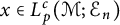 $x\in L_p^c(\mathcal {M};\mathcal {E}_n)$
,
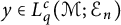 $y \in L_q^c(\mathcal {M};\mathcal {E}_n)$
, and
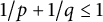 $1/p +1/q \leq 1$
. An important fact about these maps is that they are independent of p as the index p in the presentation of [Reference Junge24] was only needed to accommodate the nontracial case. Below, we will simply use
 $u_n$
for
 $u_{n,p}$
.
For
 $0<p\leq \infty $
, the range of
 $u_n$
is complemented in
 $L_p(\mathcal {M}_n,\ell _2^c)$
. In fact, as proved in [Reference Junge24, Proposition 2.8(iii)], there exists a contractive projection
 $\mathcal {Q}_{n}$
from
 $L_p(\mathcal {M}_n; \ell _2^c)$
onto the range of
 $u_{n}$
such that for every
 $\xi \in L_p(\mathcal {M}_n;\ell _2^c)$
,
 $$ \begin{align*} \mathcal{Q}_{n}(\xi)^*\mathcal{Q}_{n}(\xi)\leq \xi^*\xi. \end{align*} $$
This fact will be used in the sequel.
Let
 $\mathfrak {F}$
be the collection of all finite sequences
 $a=(a_n)_{n\geq 1}$
in
 $\mathcal {FS}$
. For
 $0<p<\infty $
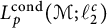
, we defined the conditioned space
 $L_p^{\text {cond}}(\mathcal {M}; \ell _2^c)$
to be the completion of the linear space
 $\mathfrak {F}$
with respect to the quasi-norm:
 $$ \begin{align} \big\| a \big\|_{L_p^{\text{cond}}(\mathcal{M}; \ell_2^c)} = \big\| \sigma_c(a)\big\|_p \end{align} $$
(here, we take
 $\mathcal {E}_0=\mathcal {E}_1$
). According to [Reference Junge24],
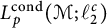 $L_p^{\text {cond}}(\mathcal {M};\ell _2^c)$
can be isometrically embedded into an
 $L_p$
-space associated to a semifinite von Neumann algebra by means of the following map:
 $$ \begin{align*} U : L_p^{\text{cond}}(\mathcal{M}; \ell_2^c) \to L_p(\mathcal{M} \overline{\otimes} B(\ell_2(\mathbb{N}^2)))\end{align*} $$
defined by setting:
 $$ \begin{align*} U((a_n)_{n\geq 1}) = \sum_{n\geq 1} u_{n-1}(a_n) \otimes e_{n,1}, \quad (a_n)_{n\geq 1} \in \mathfrak{F}. \end{align*} $$
The range of U may be viewed as a double indexed sequences
 $(x_{n,k})$
such that
 $x_{n,k} \in L_p(\mathcal {M}_n)$
for all
 $k\geq 1$
. As an operator affiliated with
 $\mathcal {M} \overline {\otimes } B(\ell _2(\mathbb {N}^2))$
, this may be expressed as
 $\sum _{n,k} x_{n,k} \otimes e_{k,1} \otimes e_{n,1}$
. It is immediate from (2.1) that if
 $(a_n)_{n\geq 1} \in \mathfrak {F}$
and
 $(b_n)_{n\geq 1} \in \mathfrak {F}$
, then
 $$ \begin{align} U( (a_n))^* U((b_n)) =\Big(\sum_{n\geq 1} \mathcal{E}_{n-1}(a_n^* b_n)\Big) \otimes e_{1,1} \otimes e_{1,1}. \end{align} $$
In particular, if
 $(a_n)_{n\geq 1} \in \mathfrak {F}$
then
 $\| (a_n) \|_{L_p^{\text {cond}}(\mathcal {M}; \ell _2^c)}=\|U( (a_n))\|_p$
and hence U is indeed an isometry.
Now, we generalize the notion of conditioned spaces to the setting of symmetric spaces of operators. This is done in steps.
 $\bullet $
Assume first that E is a symmetric quasi-Banach function space satisfying
 $L_p \cap L_\infty \subseteq E\subseteq L_p +L_\infty $
for some
 $0<p<\infty $
and
 $L_p \cap L_\infty $
is dense in E. This is the case for instance when E is a separable fully symmetric quasi-Banach function space. For a given sequence
 $a=(a_n)_{n\geq 1} \in \mathfrak {F}$
, we set:
 $$ \begin{align*} \big\| (a_n) \big\|_{E^{\text{cond}}(\mathcal{M}; \ell_2^c)} = \big\| \sigma_c(a)\big\|_{E(\mathcal{M})}=\big\| U( (a_n))\big\|_{E(\mathcal{M} \overline{\otimes} B(\ell_2(\mathbb{N}^2)))}. \end{align*} $$
This is well-defined and induces a quasi-norm on the linear space
 $\mathfrak {F}$
. We define the quasi-Banach space
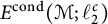 $E^{\text {cond}}(\mathcal {M}; \ell _2^c)$
to be the completion of the quasi normed space
 $(\mathfrak {F}, \|\cdot \|_{E^{\text {cond}}(\mathcal {M}; \ell _2^c)} )$
. The space
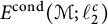 $E^{\text {cond}}(\mathcal {M};\ell _2^c)$
will be called the column conditioned space associated with E. It is clear that U extends to an isometry from
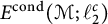 $E^{\text {cond}}(\mathcal {M};\ell _2^c)$
into
 $E(\mathcal {M} \overline {\otimes } B(\ell _2(\mathbb {N}^2)))$
which we will still denote by U.
Below, we use the notation
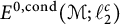 $E^{0, \textrm {cond}}(\mathcal {M}; \ell _2^c)$
for the closure of the linear space
 $\mathfrak {F}^0=\{a=(a_n) \in \mathfrak {F}: a_1=0\}$
in
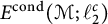 $E^{\text {cond}}(\mathcal {M}; \ell _2^c)$
. One can easily see that for
 $a=(a_n)_{n\geq 1} \in \mathfrak {F}$
, we have
 $$ \begin{align*} \max\Big\{ \big\| \mathcal{E}_1(|a_1|^2)^{1/2} \big\|_{E(\mathcal{M}_1)}, \big\| (a_n)_{n\geq 2}\big\|_{E^{\text{cond}}(\mathcal{M};\ell_2^c)} \Big\} \leq \big\| (a_n)_{n\geq 1}\big\|_{E^{\text{cond}}(\mathcal{M};\ell_2^c)}. \end{align*} $$
This shows that we have the direct sum
 $$ \begin{align} E^{\text{cond}}(\mathcal{M};\ell_2^c)= E^c(\mathcal{M};\mathcal{E}_1) \oplus E^{0, \textrm{cond}}(\mathcal{M};\ell_2^c). \end{align} $$
 $\bullet $
Assume now that
 $E\subseteq L_p +L_q$
for some
 $0<p,q<\infty $
that is not necessarily separable. We set
 $$ \begin{align*} E^{\text{cond}}(\mathcal{M}; \ell_2^c)=\big\{ x \in (L_p +L_q)^{\text{cond}}(\mathcal{M};\ell_2^c) : U(x) \in E(\mathcal{M} \overline{\otimes} B(\ell_2(\mathbb N^2)) )\big\} \end{align*} $$
equipped with the quasi-norm:
 $$ \begin{align*} \big\|x \big\|_{E^{\text{cond}}(\mathcal{M}; \ell_2^c)} =\big\| U(x) \big\|_{E(\mathcal{M} \overline{\otimes} B(\ell_2(\mathbb{N}^2)))}. \end{align*} $$
It is clear that
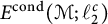 $E^{\text {cond}}(\mathcal {M}; \ell _2^c)$
as defined is a linear quasi-normed space. We claim that it is complete. Indeed, if
 $(x_\nu )_{\nu \geq 1}$
is a Cauchy sequence in
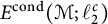 $E^{\text {cond}}(\mathcal {M}; \ell _2^c)$
, then it converges to some
 $x \in (L_p +L_q)^{\text {cond}}(\mathcal {M};\ell _2^c)$
. Since
 $( U(x_\nu ))_{\nu \geq 1}$
is also a Cauchy sequence in the quasi-Banach space
 $E(\mathcal {M} \overline {\otimes } B(\ell _2(\mathbb {N}^2)))$
and
 $E(\mathcal {M} \overline {\otimes } B(\ell _2(\mathbb {N}^2))) \subseteq (L_p +L_q)(\mathcal {M} \overline {\otimes } B(\ell _2(\mathbb {N}^2)))$
, it follows that
 $x \in E^{\text { cond}}(\mathcal {M}; \ell _2^c)$
and
 $(x_\nu )_{\nu \geq 1}$
converges to x in
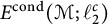 $E^{\text {cond}}(\mathcal {M}; \ell _2^c)$
. We should note here that if
 $L_p \cap L_\infty $
is dense in E then the above definition coincides with the one described in the previous bullet. We also define
 $$ \begin{align*} E^{0, \textrm{cond}}(\mathcal{M}; \ell_2^c)=(L_p +L_q)^{0, \textrm{cond}}(\mathcal{M}; \ell_2^c) \cap E^{\text{cond}}(\mathcal{M}; \ell_2^c). \end{align*} $$
The direct sum stated in (2.4) still applies.
Remark 2.2 At the time of this writing, we do not know of any suitable definition for conditioned space associated with
 $L_p + L_\infty $
when
 $0<p<2$
. It is also unclear if our definition of
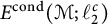 $E^{\text {cond}}(\mathcal {M};\ell _2^c)$
for non separable space
 $E\subset L_p + L_q$
when
 $0<p<2$
is independent of the isometry U.
We now recall the construction of column conditioned martingale Hardy spaces. As in the conditioned spaces, we describe the noncommutative conditioned Hardy spaces in steps. Let
 $\mathfrak {F}(M)$
be the collection of all finite martingale
 $(x_n)_{1\leq n \leq N}$
for which
 $ x_N \in \mathcal {FS}$
. We can easily see that for every
 $0<p\leq \infty $
,
 $\mathfrak {F}(M) \subseteq \mathsf {h}_p^c(\mathcal {M})$
. As in the case of conditioned spaces,
 $\mathfrak {F}(M)$
is dense in
 $\mathsf {h}_p^c(\mathcal {M})$
when
 $0<p<\infty $
.
 $\bullet $
First, assume that
 $E\subseteq L_2 + L_\infty $
. In this case, column conditioned square functions are well-defined for bounded martingales in
 $E(\mathcal {M})$
. We define
 $\mathsf {h}_E^c(\mathcal {M})$
to be the collection of all bounded martingale x in
 $E(\mathcal {M})$
for which
 $s_c(x) \in E(\mathcal {M})$
. We equip
 $\mathsf {h}_E^c(\mathcal {M})$
with the norm:
 $$ \begin{align*} \big\|x \big\|_{\mathsf{h}_E^c} = \big\|s_c(x)\big\|_{E(\mathcal{M})}. \end{align*} $$
One can easily verify that
 $(\mathsf {h}_E^c(\mathcal {M}), \|\cdot \|_{\mathsf {h}_E^c})$
is complete.
 $\bullet $
Next, we consider quasi-Banach space E such that
 $L_p\cap L_\infty $
is dense in E for some
 $0<p<\infty $
. This is the case if E is separable. Let
 $x \in \mathfrak {F}(M)$
. As noted above,
 $s_c(x) \in L_p(\mathcal {M}) \cap \mathcal {M}$
. In particular,
 $s_c(x) \in E(\mathcal {M})$
. We equip
 $\mathfrak {F}(M)$
with the quasi-norm
 $$ \begin{align*} \big\|x \big\|_{\mathsf{h}_E^c} = \big\|s_c(x)\big\|_{E(\mathcal{M})}=\big\|(dx_n)\big\|_{E^{\mathrm{cond}}(\mathcal{M};\ell_2^c)}. \end{align*} $$
The column conditioned Hardy space
 $\mathsf {h}_E^c(\mathcal {M})$
is the completion of
 $(\mathfrak {F}(M), \|\cdot \|_{\mathsf {h}_E^c})$
. Clearly, the map
 $x\mapsto (dx_n)$
(from
 $\mathfrak {F}(M)$
into
 $\mathfrak {F}$
) extends to an isometry from
 $\mathsf {h}_E^c(\mathcal {M})$
into
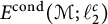 $E^{\mathrm {cond}}(\mathcal {M};\ell _2^c)$
which we denote by
 $\mathcal {D}_c$
. In particular,
 $\mathsf {h}_E^c(\mathcal {M})$
is isometrically isomorphic to a subspace of
 $E(\mathcal {M}\overline {\otimes }B(\ell _2(\mathbb {N}^2)))$
via the isometry
 $U\mathcal {D}_c$
. We should note here that if
 $L_2 \cap L_\infty $
is dense in E and
 $E\subseteq L_2 +L_\infty $
, then the two definitions provide the same space.
 $\bullet $
Assume now that
 $E \subset L_q + L_q$
for
 $0<p,q<\infty $
. As in the case of conditioned spaces, we set
 $$ \begin{align*} \mathsf{h}_E^c(\mathcal{M})=\big\{ x \in \mathsf{h}_{L_p +L_q}^c(\mathcal{M}) : U\mathcal{D}_c(x) \in E(\mathcal{M} \overline{\otimes} B(\ell_2(\mathbb N^2)) )\big\} \end{align*} $$
equipped with the quasi-norm:
 $$ \begin{align*} \big\|x \big\|_{\mathsf{h}_E^c} =\big\| U\mathcal{D}_c(x) \big\|_{E(\mathcal{M} \overline{\otimes} B(\ell_2(\mathbb{N}^2)))}. \end{align*} $$
Since the operator U is independent of the index, one can easily see that the space
 $\mathsf {h}_E^c(\mathcal {M})$
is independent of p and q. Moreover, one can verify as in the case of conditioned spaces that the quasi-normed space
 $(\mathsf {h}_E^c(\mathcal {M}), \|\cdot \|_{\mathsf {h}_E^c})$
is complete. Furthermore, if E is such that
 $L_2 \cap L_\infty $
is dense in E then
 $\mathsf {h}_E^c(\mathcal {M})$
coincides with the one defined through completion considered in the second bullet.
The following fact will be used in the sequel.
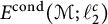
Lemma 2.3 Let
 $0<p<q<\infty $
and assume that
 $E\subseteq L_p +L_q$
. The Hardy space
 $\mathsf {h}_E^c(\mathcal {M})$
is
 $1$
-complemented in
 $E^{\mathrm {cond}}(\mathcal {M};\ell _2^c)$
. More precisely, there is an onto map
 $\Pi : E^{\mathrm {cond}}(\mathcal {M};\ell _2^c) \to \mathsf {h}_E^c(\mathcal {M})$
with
 $\|\Pi \|=1$
and
 $\Pi {\mathcal D}_c $
is the identity map in
 $\mathsf {h}_E^c(\mathcal {M})$
.
Proof Let
 $n\geq 1$
and
 $b \in \mathcal {FS}$
. Using the Kadison–Schwarz inequality for conditional expectations, we have
 $$ \begin{align} \mathcal{E}_{n-1}(|\mathcal{E}_n(b)-\mathcal{E}_{n-1}(b)|^2) \leq \mathcal{E}_{n-1}(|b|^2). \end{align} $$
We define
 $\Pi : \mathfrak {F} \to \mathsf {h}_E^c(\mathcal {M})$
by setting:
 $$ \begin{align*} a=(a_n)_{n\geq 1} \mapsto \sum_{n\geq 1} \mathcal{E}_n(a_n)- \mathcal{E}_{n-1}(a_n). \end{align*} $$
It follows from (2.5) that
 $s_c(\Pi (a)) \leq \sigma _c(a)$
for every
 $a\in \mathfrak {F}$
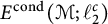
. If
 $\mathfrak {F}$
is dense in
 $E^{\mathrm {cond}}(\mathcal {M};\ell _2^c)$
, then
 $\Pi $
extends to a bounded linear map from
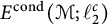 $E^{\mathrm {cond}}(\mathcal {M};\ell _2^c)$
onto
 $\mathsf {h}_E^c(\mathcal {M})$
with
 $\|\Pi : E^{\mathrm {cond}}(\mathcal {M};\ell _2^c) \to \mathsf {h}_E^c(\mathcal {M})\| \leq 1$
. Clearly, if
 $x \in \mathsf {h}_E^c(\mathcal {M})$
, we have
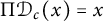 $\Pi {\mathcal D}_c (x)=x$
. This verifies the lemma for the case where E is separable.
For the general case, we observe that from the fact that
 $\mathfrak {F}$
is dense in
 $(L_p +L_q)^{\mathrm {cond}}(\mathcal {M};\ell _2^c)$
, the inequality on conditioned square functions above can be restated as:
 $$ \begin{align} \big| U{\mathcal D}_c(\Pi( y)) \big| \leq \big| U( y)\big|, \quad y\in (L_p + L_q)^{\mathrm{cond}}(\mathcal{M};\ell_2^c). \end{align} $$
If
 $y \in E^{\mathrm {cond}}(\mathcal {M};\ell _2^c)$
, then by definition
 $y \in (L_p +L_q)^{\mathrm {cond}}(\mathcal {M};\ell _2^c)$
and
 $U(y) \in E(\mathcal {M} \overline {\otimes } B(\ell _2(\mathbb {N}^2)))$
. By the separable case,
 $\Pi (y) \in \mathsf {h}_{L_p +L_q}^c(\mathcal {M})$
. Moreover, it follows from (2.6) that
 $U{\mathcal D}(\Pi (y)) \in E(\mathcal {M} \overline {\otimes } B(\ell _2(\mathbb {N}^2)))$
. This means,
 $\Pi (y)\in \mathsf {h}_E^c(\mathcal {M})$
with
 $\|\Pi (y)\|_{\mathsf {h}_E^c}\leq \| y\|_{E^{\mathrm {cond}}(\mathcal {M};\ell _2^c)}$
. ▪
We refer to [Reference Cadilhac and Ricard6, Reference Dirksen11, Reference Jiao19, Reference Jiao, Sukochev, Zanin and Zhou22, Reference Junge and Xu26, Reference Randrianantoanina and Wu42, Reference Randrianantoanina, Wu and Xu43] for more information on noncommutative Hardy spaces associated with symmetric spaces of measurable operators. In the sequel, noncommutative column Hardy spaces associated with Orlicz space
 $L_\Phi $
will be denoted by
 $\mathcal {H}_\Phi ^c(\mathcal {M})$
and
 $\mathsf {h}_\Phi ^c(\mathcal {M})$
while those associated with the Lorentz space
 $L_{p,q}$
will be denoted by
 $\mathcal {H}_{p,q}^c(\mathcal {M})$
and
 $\mathsf {h}_{p,q}^c(\mathcal {M})$
.
We conclude this subsection with a description of the dual space of the Hardy space
 $\mathsf {h}_1^c(\mathcal {M})$
. A martingale x belongs to the column little bmo space denoted by
 $\mathsf {bmo}^c(\mathcal {M})$
if
 $$ \begin{align*} \big\| x \big\|_{\mathsf{bmo}^c}= \max\Big\{ \big\|x_1\big\|_\infty; \mathop{\mathrm{sup}}_{m} \mathop{\mathrm{sup}}_{1\leq n\leq m }\big\| \mathcal{E}_n(|x_m-x_n|^2) \big\|_\infty^{1/2} \Big\} <\infty. \end{align*} $$
The Banach space
 $(\mathsf {bmo}^c(\mathcal {M}), \|\cdot \|_{\mathsf {bmo}^c})$
was introduced in [Reference Perrin33] for finite case where it was shown that it coincides with the dual of the Hardy space
 $\mathsf {h}_1^c(\mathcal {M})$
. The proof given there can be easily generalized to the semifinite case. We record this for further use:
 $$ \begin{align} (\mathsf{h}_1^c(\mathcal{M}))^* =\mathsf{bmo}^c(\mathcal{M}) \end{align} $$
with equivalent norms.
2.3 Atomic decompositions for martingale Orlicz–Hardy spaces
In this subsection, we will analyze conditioned spaces and conditioned Hardy spaces associated with Orlicz spaces. More specifically, we will describe a type of atomic decomposition in the context of Orlicz spaces. Results from this subsection play key role in the next section. Toward this end, we will start from setting up some notations.
Throughout this subsection, we always assume that
 $0<p \leq q <2$
and
 $\Phi $
is an Orlicz function that is p-convex and q-concave. First, we fix a positive Borel measure
 $\mu $
on the interval
 $[0,\infty )$
so that:
 $$ \begin{align} \Phi(t)\approx_{p,q}\int_0^\infty \min\{(ts)^p, (ts)^q\} \ d\mu(s). \end{align} $$
The existence of such integral representation was proved for convex functions (see the proof of [Reference Jiao, Sukochev and Zanin21, Lemma 6.2]). The argument given in [Reference Jiao, Sukochev and Zanin21] can be readily adjusted to include the more general case of p-convex functions when
 $0<p<1$
.
Next, we fix an Orlicz function
 $\Theta $
so that
 $L_\Phi $
admits the factorization:
 $$ \begin{align} L_\Phi=L_2 \odot L_\Theta, \end{align} $$
where the product
 $L_2 \odot L_\Theta $
is the collection of all function f that admit factorization
 $f=gh$
with
 $g\in L_2$
and
 $h\in L_{\Theta }$
. The quasi-norm on
 $L_2\odot L_\Theta $
is given by:
 $$ \begin{align*} \big\|f\big\|_{L_2 \odot L_\Theta} :=\inf\left\{\big\|g\big\|_{L_2}\big\|h \big\|_{L_\Theta}: g\in L_2, h\in L_\Theta, f=gh\right\}. \end{align*} $$
We note that the Orlicz function
 $\Theta $
can be taken to be the inverse of the function
 $t\mapsto t^{-1/2}\Phi ^{-1}(t)$
for
 $t>0$
. We refer to [Reference Maligranda31] for more details.
We will also make use of the following function:
 $$ \begin{align} \Psi(t)= \int_0^\infty (t^{2-p}s^{-p} + t^{2-q}s^{-q})^{-1}\ d\mu(s), \end{align} $$
where
 $\mu $
is the positive Borel measure from the representation of
 $\Phi $
in (2.8). The reason for the consideration of
 $\Psi $
is summarized in the next lemma. The first three items are straightforward generalizations of [Reference Randrianantoanina, Wu and Zhou44, Proposition 3.3], whereas the last item can be deduced as in [Reference Randrianantoanina, Wu and Zhou44, Lemma 3.4].
Lemma 2.4
-
(i)
 $\Psi (t) \approx _{p,q} t^{-2} \Phi (t)$
;
-
(ii)
$\Theta \big ( \Psi (t)^{-1/2}\big ) \approx _{p,q} \Phi (t)$
; -
(iii)
$t \mapsto \Psi (t^{1/2})$
is operator monotone decreasing; and -
(iv) for any increasing sequence of positive operators
$a_n \uparrow a$
, we have:
$$ \begin{align*} \sum_{n\geq 1} \tau\big( (a_{n+1}^2-a_n^2) \Psi(a_{n+1})\big) \lesssim_{p,q} \tau\big(\Phi(a)\big). \end{align*} $$




We now introduce a concept of atoms for conditioned space constructed from the Orlicz function space
 $L_\Phi $
.
Definition 2.5 A sequence
 $x \in L_\Phi (\mathcal {M};\ell _2^c)$
is called an algebraic
 $L_\Phi ^{c, \textrm {cond}}$
-atom if it admits a factorization
 $x=\alpha \ .\ \beta $
where
-
(i)
$\alpha = \sum _{j<n} \alpha _{n,j} \otimes e_{n,j}$
is a strictly lower triangular matrix in
$L_2(\mathcal {M} \overline {\otimes } B(\ell _2(\mathbb N)))$
with
$$ \begin{align*} \big\|\alpha\big\|_2 =\left( \sum_{j<n} \|\alpha_{n,j}\|_2^2 \right)^{1/2} \leq 1. \end{align*} $$
-
(ii)
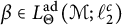
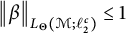
$\beta \in L_{\Theta }^{\mathrm {ad}}(\mathcal {M};\ell _2^c)$
with
$\big \| \beta \big \|_{L_\Theta (\mathcal {M};\ell _2^c)}\leq 1$
.



The above definition was motivated by the case of
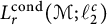 $L_r^{\mathrm {cond}}(\mathcal {M};\ell _2^c)$
for
 $1\leq r<2$
introduced for the first time in [Reference Perrin34] and explored further in [Reference Hong, Junge and Parcet17]. We also refer to [Reference Chen, Randrianantoanina and Xu7] where the same concept was considered for the case of conditioned Hardy space
 $\mathsf {h}_r^c(\mathcal {M})$
for the range
 $0<r\leq 1$
. More recently, the case of Orlicz-conditioned Hardy space
 $\mathsf {h}_\varphi ^c(\mathcal {M})$
associated with convex Orlicz function
 $\varphi $
was formulated in [Reference Randrianantoanina, Wu and Zhou44] in the context of
 $\varphi $
-moments.
We should note that since strictly lower triangular matrices were used in the definition of algebraic atoms, it follows that if
 $x=(x_n)_{n\geq 1}$
is an algebraic
 $L_\Phi ^{c, \textrm {cond}}$
-atom then
 $x_1=0$
.
The next lemma can be deduced as in the first part of [Reference Perrin34, Theorem 3.6.10] using the factorization
 $L_\Phi =L_2 \odot L_\Theta $
. We include the argument for the sake of completeness.
Lemma 2.6 Every algebraic
 $L_\Phi ^{c, \textrm {cond}}$
-atom belongs to
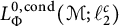 $L_\Phi ^{0, \textrm {cond}}(\mathcal {M};\ell _2^c)$
. More precisely, if x is an algebraic
 $L_\Phi ^{c, \textrm {cond}}$
-atom then
 $\displaystyle { \|x \|_{L_{\Phi }^{\mathrm {cond}}(\mathcal {M};\ell _2^c)} \leq 1}$
.
Proof Let
 $x=\alpha \ .\ \beta $
be an algebraic
 $L_\Phi ^{c, \textrm {cond}}$
-atom. As observed earlier,
 $x_1=0$
and for
 $n\geq 2$
,
 $x_n= \sum _{j<n} \alpha _{n,j} \beta _j$
. Since
 $\beta $
is adapted, it follows that
 $$ \begin{align*} \mathcal{E}_{n-1}|x_n|^2 =\sum_{m,j<n} \beta_m^* \mathcal{E}_{n-1}(\alpha_{n,m}^* \alpha_{n,j}) \beta_j. \end{align*} $$
From the property of the module map
 $u_{n-1}$
, we have
 $$ \begin{align*} \mathcal{E}_{n-1}|x_n|^2 \otimes e_{1,1} &= \sum_{m,j <n} (\beta_m^* \otimes e_{1,1}). u_{n-1}(\alpha_{n,m})^* u_{n-1}(\alpha_{n,j}). (\beta_j \otimes e_{1,1}) \\ &=| \sum_{j<n} u_{n-1}(\alpha_{n,j}).(\beta_j \otimes e_{1,1})|^2. \end{align*} $$
This implies that
 $$ \begin{align*} \sigma_c^2(x) \otimes e_{1,1} =\sum_{n\geq 2} | \sum_{j<n} u_{n-1}(\alpha_{n,j}).(\beta_j \otimes e_{1,1})|^2. \end{align*} $$
We write further that
 $$ \begin{align*} \sigma_c^2(x) \otimes e_{1,1} \otimes e_{1,1} =| \sum_{n\geq 2} \sum_{j<n} [u_{n-1}(\alpha_{n,j}).(\beta_j \otimes e_{1,1})] \otimes e_{n,1} |^2. \end{align*} $$
This allows us to deduce that
 $$ \begin{align*} \sigma_c(x) \otimes e_{1,1} \otimes e_{1,1} = \big|\big(u_{n-1}(\alpha_{n,j}) \big)_{j<n}. \ \sum_{k\geq 1} \beta_k \otimes e_{1,1} \otimes e_{k,1} \big|, \end{align*} $$
where the strictly lower triangular matrix
 $\widehat {\alpha }=(\big (u_{n-1}(\alpha _{n,j}) )_{j<n}$
takes its values in
 $L_2(\mathcal {M} \overline {\otimes } B(\ell _2(\mathbb {N})))$
. We may view
 $\widehat {\alpha }$
as an operator affiliated with
 $\mathfrak {M}=\mathcal {M} \overline {\otimes } B(\ell _2(\mathbb {N}))) \overline {\otimes } B(\ell _2(\mathbb {N})))$
. If
 $\mu (\cdot )$
denote the generalized singular number relative to
 $\mathfrak {M}$
equipped with its natural trace, then
 $$ \begin{align*} \big\| \sigma_c(x)\big\|_{L_\Phi(\mathcal{M})} = \|\mu(\sigma_c(x) \otimes e_{1,1} \otimes e_{1,1}) \big\|_{L_\Phi}. \end{align*} $$
It follows from [Reference Fack and Kosaki12, Theorem 4.2] that
 $$ \begin{align*} \big\| \sigma_c(x)\big\|_{L_\Phi(\mathcal{M})} &\leq \|\mu(\widehat{\alpha}) \big\|_{2} .\big\| \mu\big( \sum_{k\geq 1} \beta_k \otimes e_{1,1} \otimes e_{k,1}\big) \big\|_{L_\Theta}\\ &= \big\| \widehat{\alpha}\big\|_{2}. \big\| \big(\sum_{k\geq 1} |\beta_k|^2\big)^{1/2} \big\|_{L_\Theta}\\ &\leq \big(\sum_{j<n} \| \alpha_{n,j}\|_2^2 \big)^{1/2}. \big\| \big(\sum_{k\geq 1} |\beta_k|^2\big)^{1/2} \big\|_{L_\Theta}. \end{align*} $$
This proves that
 $\| x \|_{L_\Phi ^{\mathrm {cond}}(\mathcal {M};\ell _2^c)}\leq 1$
. ▪
Using the above notion of atoms, we may naturally consider the following concept of atomic decompositions:
Definition 2.7 A sequence
 $x \in L_\Phi (\mathcal {M};\ell _2^c)$
is said to admit an algebraic
 $L_\Phi ^{c, \textrm {cond}}$
-atomic decomposition if
 $$ \begin{align*} x =\sum_{k} \lambda_k a^{(k)}, \end{align*} $$
where for each k,
 $a^{(k)}$
is either an algebraic
 $L_\Phi ^{c, \textrm {cond}}$
-atom or
 $a^{(k)}$
belongs to the unit ball of the conditioned space
 $L_\Phi ^c(\mathcal {M};\mathcal {E}_1)$
and
 $\lambda _k \in \mathbb {C}$
satisfying
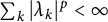 $\sum _k|\lambda _k|^p <\infty $
for
 $0<p<1$
and
 $\sum _k|\lambda _k| <\infty $
for
 $1\leq p<2$
. Since
 $\Phi $
is p-convex and algebraic
 $L_\Phi ^{c, \textrm {cond}}$
-atoms belong to the unit ball of
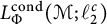 $L_\Phi ^{\mathrm {cond}}(\mathcal {M};\ell _2^c)$
, it follows that if x admits an algebraic
 $L_\Phi ^{c, \textrm {cond}}$
-atomic decomposition then it belongs to
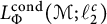 $L_\Phi ^{\mathrm {cond}}(\mathcal {M};\ell _2^c)$
.
Following [Reference Perrin34], the corresponding algebraic atomic column conditioned space
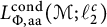 $L_{\Phi ,\mathrm {aa}}^{ \textrm {cond}}(\mathcal {M};\ell _2^c)$
is defined to be the completion of the space of all x that admit algebraic
 $L_\Phi ^{c, \textrm {cond}}$
-atomic decompositions in the space
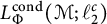 $L_\Phi ^{\mathrm {cond}}(\mathcal {M};\ell _2^c)$
. If x admits an algebraic
 $L_\Phi ^{c, \textrm {cond}}$
-atomic decomposition, we set:
 $$ \begin{align*} \|x\|_{L_{\Phi,\mathrm{aa}}^{\mathrm{cond}}(\mathcal{M};\ell_2^c)}=\inf\Big(\sum_k |\lambda_k|^p\Big)^{1/p} \quad \text{for} \ 0<p\leq 1\end{align*} $$
and
 $$ \begin{align*} \|x\|_{L_{\Phi,\mathrm{aa}}^{\mathrm{cond}}(\mathcal{M};\ell_2^c)}=\inf\sum_k |\lambda_k| \quad \text{for} \ 1<p<2,\end{align*} $$
where the infimum is taken over all decompositions of x as described above. We refer the reader to [Reference Chen, Randrianantoanina and Xu7] for a more in-depth discussion on the need to separate the two cases.
The following result generalizes the atomic decomposition of conditioned
 $L_p$
-spaces from [Reference Perrin34] in two directions: it is valid for Orlicz spaces and also cover the quasi-Banach space range. This will play a crucial role in the next section. The approach of [Reference Perrin34] was by duality which is not applicable to the present situation since we are dealing with not necessarily convex functions. Our constructive proof given below combined ideas from [Reference Chen, Randrianantoanina and Xu7] and the case of Hardy spaces associated with convex Orlicz functions considered in [Reference Randrianantoanina, Wu and Zhou44]. This may be of independent interest.
Theorem 2.8 Let
 $\Phi $
be p-convex and q-concave for
 $0<p\leq q<2$
. Then the two spaces
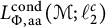 $ L_{\Phi ,\mathrm {aa}}^{ \textrm {cond}}(\mathcal {M};\ell _2^c)$
and
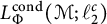 $ L_\Phi ^{\mathrm {cond}}(\mathcal {M};\ell _2^c)$
coincide (with constant of isomorphism depending only on p and q).
More precisely, every
 $ x \in \mathfrak {F}^0$
admits a factorization
 $x= \alpha \, .\, \beta $
where
 $\alpha $
is a strictly lower triangular matrix in
 $L_2(\mathcal {M} \overline {\otimes } B(\ell _2(\mathbb {N})))$
and
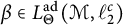 $\beta \in L_\Theta ^{\mathrm {ad}}(\mathcal {M},\ell _2^c)$
satisfying:
 $$ \begin{align*} \big\| \alpha\big\|_2 \, .\, \big\| \beta\big\|_{L_\Theta(\mathcal{M};\ell_2^c)} \lesssim_{p,q} \big\| x \big\|_{L_\Phi^{\mathrm{cond}}(\mathcal{M};\ell_2^c)}. \end{align*} $$
Proof First, we recall from earlier discussion that
 $L_{\Phi ,\mathrm {aa}}^{ \textrm {cond}}(\mathcal {M};\ell _2^c) \subseteq L_\Phi ^{\mathrm {cond}}(\mathcal {M};\ell _2^c)$
. Thus, we only need to verify one inclusion. This will be deduced from the second part of the theorem.
Let
 $ x=(x_n)_{n=1}^N \in \mathfrak {F}^0$
. The construction below is an adaptation of the argument used in [Reference Randrianantoanina, Wu and Zhou44]. By definition,
 $x_1=0$
and there exists a projection
 $e\in \mathcal {M}_1$
with
 $\tau (e)<\infty $
such that for
 $2\leq n\leq N$
,
 $x_n=ex_n e$
.
First, we note that for
 $j\geq 2$
, we have
 $\sigma _{c,j}(x) \in e\mathcal {M}_{j-1}e$
. By approximation, we may assume that each of the
 $\sigma _{c,j}(x)$
s is invertible with bounded inverse in
 $e\mathcal {M} e$
. Below, we simply write
 $\sigma _j$
for
 $\sigma _{c,j}(x)$
and the function
 $\Psi $
is as defined in (2.10). Let
 $\lambda>0$
to be determined later. For
 $n\geq 2$
, we write
 $$ \begin{align*} x_n &=x_n \Psi(\lambda\sigma_n)\Psi(\lambda\sigma_n)^{-1}\\ &=x_n\Psi(\lambda\sigma_n)\big[ \Psi(\lambda\sigma_2)^{-1} + \sum_{3\leq m\leq n} \Psi(\lambda\sigma_m)^{-1}-\Psi(\lambda\sigma_{m-1})^{-1}\big]\\ &=x_n \Psi(\lambda\sigma_n)\Psi(\lambda\sigma_2)^{-1} + \sum_{2\leq j<n} x_n \Psi(\lambda\sigma_n)\big(\Psi(\lambda\sigma_{j+1})^{-1} -\Psi(\lambda\sigma_j)^{-1}\big). \end{align*} $$
We define the strictly lower triangular matrix
 $\alpha $
by setting:
 $$ \begin{align} \begin{cases} \alpha_{n,1} &:=x_n\Psi(\lambda\sigma_n)\Psi(\lambda\sigma_2)^{-1/2};\\ \alpha_{n,j}&:=\displaystyle{x_n\Psi(\lambda\sigma_n)\left(\Psi(\lambda\sigma_{j+1})^{-1}-\Psi(\lambda\sigma_{j})^{-1}\right)^{1/2},\quad\text{for }2 \leq j<n.} \end{cases} \end{align} $$
We should point out here that since the function
 $t\mapsto \Psi (t^{1/2})$
is operator monotone decreasing and
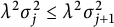 $\lambda ^2\sigma _{j}^2 \leq \lambda ^2 \sigma _{j+1}^2$
, we have
 $\Psi (\lambda \sigma _{j+1}) \leq \Psi (\lambda \sigma _{j})$
. Taking inverses,
 $\Psi (\lambda \sigma _{j+1})^{-1}-\Psi (\lambda \sigma _{j})^{-1}\geq 0$
. Thus, taking
 $1/2$
-power in the expression above is justified.
The column sequence is defined by setting:
 $$ \begin{align} \begin{cases} \beta_{1,1} &:=\displaystyle{\Psi(\lambda\sigma_2)^{-1/2};}\\ \beta_{m,1}&:=\displaystyle{\left(\Psi(\lambda\sigma_{m+1})^{-1}-\Psi(\lambda\sigma_{m})^{-1}\right)^{1/2}, \quad \text{for }m\geq 2}. \end{cases} \end{align} $$
Then
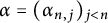 $\alpha =(\alpha _{n,j})_{j<n}$
is a strictly lower triangular matrix and
 $\beta =(\beta _{m,1})_{m\geq 1}$
is an adapted sequence. Moreover, for every
 $n\geq 2$
, it clearly follows from the definition that
 $$ \begin{align*} (\alpha.\beta)_{n,1}= \sum_{j\geq 1} \alpha_{n,j}. \beta_{j,1}=x_n. \end{align*} $$
That is, we have the factorization
 $x= \alpha \, .\, \beta $
. We claim that the product
 $\alpha \,. \, \beta $
satisfies the desired norm estimate. We begin with the
 $L_2$
-norm of
 $\alpha $
.
 $$ \begin{align*} \big\|\alpha\big\|_2^2 &=\sum_{n\geq 2} \sum_{1\leq j<n} \big\|\alpha_{n,j}\big\|_2^2\\ &=\sum_{n\geq 2} \tau\big(\Psi(\lambda\sigma_n) |x_n|^2 \Psi(\lambda\sigma_n) \big[ \Psi(\lambda\sigma_2)^{-1} +\sum_{2\leq j<n} \Psi(\lambda\sigma_{j+1})^{-1}-\Psi(\lambda\sigma_j)^{-1}\big]\big)\\ &=\sum_{n\geq 2}\tau\big(|x_n|^2\Psi(\lambda\sigma_n)\big). \end{align*} $$
Since
 $(\Psi (\lambda \sigma _n))$
is a predictable sequence, we have
 $$ \begin{align*} \big\|\alpha\big\|_2^2&=\sum_{n\geq 2} \tau\big(\mathcal{E}_{n-1}(|x_n|^2) \Psi(\lambda\sigma_n) \big)\\ &=\sum_{n\geq 2} \tau\big( (\sigma_n^2- \sigma_{n-1}^2)\Psi(\lambda\sigma_n)\big)\\ &=\lambda^{-2}\sum_{n\geq 2} \tau\big( ((\lambda\sigma_n)^2-(\lambda \sigma_{n-1})^2)\Psi(\lambda\sigma_n)\big). \end{align*} $$
We may deduce from Lemma 2.4(iv) that there is a constant
 $C_{p,q}$
so that
 $$ \begin{align} \big\|\alpha\big\|_2^2 \leq C_{p,q} \lambda^{-2} \tau\big(\Phi(\lambda\sigma_c(x))\big). \end{align} $$
On the other hand, Lemma 2.4(ii) implies that there exists a constant
 $C_{p,q}'$
so that
 $$ \begin{align} \tau\Big[ \Theta\Big( \big(\sum_{m\geq 1} |\beta_{m,1}|^2\big)^{1/2} \Big)\Big] =\tau \Big[ \Theta\Big( \Psi (\lambda\sigma_c(x))^{-1/2} \Big)\Big] \leq C_{p,q}'\tau\big(\Phi(\lambda\sigma_c(x))\big). \end{align} $$
Let
 $K_{p,q}=\max \{C_{p,q}, C_{p,q}'\} +1$
. Since
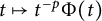 $t\mapsto t^{-p}\Phi (t)$
is nondecreasing, one can easily verify that
 $\Phi (t)\leq K_{p,q}^{-1} \Phi (K_{p,q}^{1/p}t)$
. Using this fact, we get from (2.13) and (2.14) that
 $$ \begin{align*} \big\|\alpha\big\|_2^2 \leq \lambda^{-2} \tau\big(\Phi( K_{p,q}^{1/p}\lambda\sigma_c(x))\big) \end{align*} $$
and
 $$ \begin{align*} \tau\left[ \Theta\left( \left(\sum_{m\geq 1} |\beta_{m,1}|^2\right)^{1/2} \right)\right] \leq \tau\big(\Phi( K_{p,q}^{1/p}\lambda\sigma_c(x))\big). \end{align*} $$
Choose
 $\lambda $
so that
 $\tau \big (\Phi ( K_{p,q}^{1/p}\lambda \sigma _c(x))\big )\leq 1$
. This can be achieved with
 $\lambda ^{-1}= K_{p,q}^{1/p} \big \|\sigma _c(x) \big \|_{L_\Phi (\mathcal {M})}$
. With the above choice of
 $\lambda $
, we clearly have
 $ \big \| \alpha \big \|_2 \leq K_{p,q}^{1/p} \big \| x \big \|_{L_\Phi ^{\mathrm {cond}}(\mathcal {M};\ell _2^c)}$
and
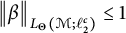 $\big \|\beta \big \|_{L_\Theta (\mathcal {M};\ell _2^c)} \leq 1$
. This proves the desired estimate and therefore the second part of the theorem.
To conclude the proof, we apply the case of
 $\mathfrak {F}^0$
with the direct sum (2.4). We see that every
 $y \in \mathfrak {F}$
admits an algebraic
 $L_\Phi ^{c, \textrm {cond}}$
-atomic decomposition with
 $\|y\|_{L_{\Phi ,\mathrm {aa}}^{\mathrm {cond}}(\mathcal {M};\ell _2^c)} \lesssim _{p,q} \|y\|_{L_\Phi ^{\mathrm {cond}}(\mathcal {M};\ell _2^c)}$
. Since
 $\mathfrak {F}$
is dense in
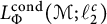 $L_\Phi ^{\mathrm {cond}}(\mathcal {M};\ell _2^c)$
, it follows that
 $L_{\Phi ,\mathrm {aa}}^{\mathrm {cond}}(\mathcal {M};\ell _2^c)=L_\Phi ^{\mathrm {cond}}(\mathcal {M};\ell _2^c)$
. ▪
Remark 2.9 Using
 $\lambda =1$
in the proof above, we also obtain a moment version of the preceding theorem: given a sequence
 $x=(x_n)_{n\geq 1} \in \mathfrak {F}^0$
, the column matrix
 $\overline {x}=\sum _{n\geq 1} x_n \otimes e_{n,1}$
admits a factorization
 $\overline {x}=\alpha \ .\ \beta $
with
 $\alpha $
is a strictly lower triangular in
 $L_2(\mathcal {M} \overline {\otimes } B(\ell _2(\mathbb N)))$
and
 $\beta $
is an adapted column matrix satisfying
 $$ \begin{align*} \big\|\alpha\big\|_2 + \tau\left[\Theta\left( \left(\sum_{n\geq 1} |\beta_{n,1}|^2 \right)^{1/2}\right)\right] \lesssim_{p,q} \tau\big[\Phi\big( \sigma_c(x)\big)\big]. \end{align*} $$
We consider now the version of algebraic atomic decomposition for martingale Hardy spaces. The next consideration generalizes notions from [Reference Chen, Randrianantoanina and Xu7, Reference Randrianantoanina, Wu and Zhou44] for non-necessarily convex Orlicz functions.
Definition 2.10 Let
 $0<p< q<2$
and
 $\Phi $
be an Orlicz function that is p-convex and q-concave. An operator
 $x \in L_\Phi (\mathcal {M})$
is called an algebraic
 $\mathsf {h}_\Phi ^c$
-atom, whenever it can be written in the form
 $x=\sum _{n\geq 1} y_nb_n$
, with
 $y_n$
and
 $b_n$
satisfying the following conditions:
-
(i)
$\mathcal {E}_n (y_n) =0$
and
$b_n \in L_\Theta (\mathcal {M}_n)$
for all
$n\geq 1$
and -
(ii)
$\displaystyle {\sum _{n\geq 1} \big \|y_n\big \|_2^2 \leq 1}$
and
$\displaystyle {\Big \| \Big ( \sum _{n\geq 1} |b_n|^2 \Big )^{1/2}\Big \|_{L_\Theta (\mathcal {M})} \leq 1}$
.



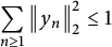
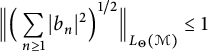
Following [Reference Chen, Randrianantoanina and Xu7, Reference Randrianantoanina, Wu and Zhou44], this concept of atoms naturally leads to the consideration of the corresponding atomic decomposition for conditioned Orlicz–Hardy spaces: we say that an operator
 $x \in L_\Phi (\mathcal {M})$
admits an algebraic
 $\mathsf {h}_\Phi ^c$
-atomic decomposition if
 $$ \begin{align*} x =\sum_{k} \lambda_k a_k, \end{align*} $$
where for each k,
 $a_k$
is an algebraic
 $\mathsf {h}_\Phi ^c$
-atom or an element of the unit ball of
 $L_\Phi (\mathcal {M}_1)$
, and
 $\lambda _k \in \mathbb {C}$
satisfying
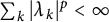 $\sum _k|\lambda _k|^p <\infty $
for
 $0<p \leq 1$
and
 $\sum _k|\lambda _k|<\infty $
for
 $1<p<2$
. The corresponding algebraic atomic column martingale Hardy space
 $\mathsf {h}_{\Phi ,\mathrm {aa}}^c(\mathcal {M})$
is defined to be the space of all x which admit a algebraic
 $\mathsf {h}_\Phi ^c$
-atomic decomposition and is equipped with
 $$ \begin{align*} \|x\|_{\mathsf{h}_{\Phi,\mathrm{aa}}^c}=\inf\Big(\sum_k |\lambda_k|^p\Big)^{1/p} \quad \text{for }0<p\le1 \end{align*} $$
and
 $$ \begin{align*} \|x\|_{\mathsf{h}_{\Phi,\mathrm{aa}}^c}=\inf\,\sum_k |\lambda_k| \quad \text{for }1< p<2, \end{align*} $$
where the infimum are taken over all decompositions of x as described above.
We note that the above concepts were introduced in [Reference Randrianantoanina, Wu and Zhou44] for the case where
 $\Phi $
is a convex function. Our main focus here is the case where
 $\Phi $
is p-convex with
 $0<p<1$
.
The next result is an extension of [Reference Chen, Randrianantoanina and Xu7, Theorem 3.10] to the case of Orlicz function spaces. It follows immediately from Theorem 2.8 and the complementation result stated in Lemma 2.3.
Corollary 2.11 Let
 $0<p<q<2$
and
 $\Phi $
is an Orlicz function that is p-convex and q-concave. Then
 $$ \begin{align*} \mathsf{h}_\Phi^{c}(\mathcal{M})= \mathsf{h}_{\Phi,\mathrm{aa}}^c(\mathcal{M}). \end{align*} $$
More precisely, if
 $ x \in \mathsf {h}_\Phi ^c(\mathcal {M})$
, then x admits a unique decomposition
 $x=x_1 +y$
where
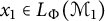 $x_1 \in L_\Phi (\mathcal {M}_1)$
and y is a scalar multiple of an algebraic
 $\mathsf {h}_{\Phi }^c$
-atom.
Indeed, if
 $\Pi : L_\Phi ^{\mathrm {cond}}(\mathcal {M};\ell _2^c) \to \mathsf {h}_\Phi ^c(\mathcal {M})$
denotes the norm one projection described in Lemma 2.3 and
 $x=\alpha \,. \, \beta $
is a algebraic
 $L_\Phi ^{c,{ \textrm {cond}}}$
-atom with
 $\alpha $
being a strictly lower triangular matrix in
 $L_2(\mathcal {M} \overline {\otimes } B(\ell _2(\mathbb N)))$
and
 $\beta $
is an adapted column matrix in
 $L_{\Theta }(\mathcal {M};\ell _2^c)$
, then we have
 $$ \begin{align*} \Pi(x) &= \sum_n \sum_{n>k} d_n(\alpha_{n,k}) \beta_{k,1}\\ &=\sum_k \left(\sum_{n>k} d_n(\alpha_{n,k}) \right) \beta_{k,1}\\ &=\sum_k a_k \beta_{k,1}. \end{align*} $$
Clearly, we have for every
 $ k\geq 1$
,
 $\mathcal {E}_k(a_k)=0$
. Moreover,
 $\sum _{k\geq 1} \|a_k\|_2^2 \leq \|\alpha \|_2^2$
. This shows in particular that
 $\Pi (x)$
is an algebraic
 $\mathsf {h}_\Phi ^c$
-atom. The assertions in the corollary follow from combining this fact with Theorem 2.8 and direct sum. ▪
We conclude this section with a companion of Theorem 2.8 for spaces of adapted sequences. It may be viewed as the algebraic atomic decompositions for spaces of adapted sequences. This will be used in the next section.
Proposition 2.12 Let
 $\Phi $
be a p-convex and q-concave Orlicz function for
 $0<p<q<2$
. If
 $x=(x_n)_{n\geq 1}$
is a sequence in
 $L_\Phi ^{\mathrm {ad}}(\mathcal {M};\ell _2^c)$
then there exists a sequence
 $\beta =(\beta _n)_{n\geq 1}$
in
 $L_\Theta ^{\mathrm {ad}}(\mathcal {M};\ell _2^c)$
and a lower triangular matrix
 $\alpha $
with the following properties:
-
(i)
$\alpha \in L_2(\mathcal {M}\overline {\otimes } B(\ell _2(\mathbb N)))$
; -
(ii) for every
$1\leq j\leq n$
,
$\alpha _{n,j} \in L_2(\mathcal {M}_n)$
; -
(iii)
$x=\alpha \,. \, \beta $
; and -
(iv)
$\big \|\alpha \big \|_2 \,. \, \big \|\beta \big \|_{L_\Theta (\mathcal {M};\ell _2^c)} \lesssim _{p,q} \big \| x\big \|_{L_\Phi (\mathcal {M};\ell _2^c)}$
.





Conversely, any sequence x admitting a factorization as above belongs to
 $L_\Phi ^{\mathrm {ad}}(\mathcal {M};\ell _2^c)$
with
 $$ \begin{align*} \big\| x\big\|_{L_\Phi(\mathcal{M};\ell_2^c)} \leq \big\|\alpha \big\|_2 \,. \, \big \|\beta \big\|_{L_\Theta(\mathcal{M};\ell_2^c)}. \end{align*} $$
First, we note that since square functions are well-defined for elements of
 $L_\Phi ^{\mathrm {ad}}(\mathcal {M}; \ell _2^c)$
, reduction to finite sequences or sequences of finite supports is not necessary.
Proof Let
 $x=(x_n)_{n\geq 1}\in L_\Phi ^{\mathrm {ad}}(\mathcal {M};\ell _2^c)$
. The construction is an adaptation of the proof of Theorem 2.8 but using square functions in place of conditioned square functions.
For each
 $n\geq 1$
,
 $\mathcal {S}_{c,n}(x) \in L_{\Phi }(\mathcal {M}_n)$
. That is,
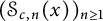 $(\mathcal {S}_{c,n}(x))_{n\geq 1}$
is an adapted sequence. We simply write
 $\varsigma _n$
for
 $\mathcal {S}_{c,n}(x)$
. As before, we may assume that the
 $\varsigma _n$
s are invertible with bounded inverse. Similarly,
 $(\Psi (\varsigma _n))_{n\geq 1}$
is an adapted sequence with the
 $\Psi (\varsigma _n)$
s being invertible.
As in the proof of Theorem 2.8, fix
 $\lambda>0$
and set
 $$ \begin{align*} \begin{cases} \alpha_{n,1} &:=x_n\Psi(\lambda\varsigma_n)\Psi(\lambda\varsigma_1)^{-1/2};\\ \alpha_{n,j}&:=\displaystyle{x_n\Psi(\lambda\varsigma_n)\left(\Psi(\lambda\varsigma_{j})^{-1}-\Psi(\lambda\varsigma_{j-1})^{-1}\right)^{1/2},\quad\text{for } 2 \leq j \leq n} \end{cases} \end{align*} $$
and
 $$ \begin{align*} \begin{cases} \beta_{1,1} &:=\displaystyle{\Psi(\lambda\varsigma_1)^{-1/2};}\\ \beta_{m,1}&:=\displaystyle{\left(\Psi(\lambda\varsigma_{m})^{-1}-\Psi(\lambda\varsigma_{m-1})^{-1}\right)^{1/2}, \quad \text{for }m\geq 2}. \end{cases} \end{align*} $$
A slight difference here is that unlike in the proof of Theorem 2.8, we do not make the indexing shift. The factorization
 $x=\alpha \, .\, \beta $
is straightforward. Clearly,
 $(\beta _{m,1})_{m\geq 1}$
is an adapted sequence. Moreover, as
 $x_n \in L_\Phi (\mathcal {M}_n)$
, it follows that
 $\alpha _{n,j}$
is affiliated with
 $\mathcal {M}_n$
and
 $(\alpha _{n,j})_{1\leq j\leq n}$
is a lower triangular matrix.
We may choose
 $\lambda $
exactly as in the proof of Theorem 2.8. That is,
 $\lambda ^{-1}=K_{p,q}^{1/p} \| \mathcal {S}_c(x) \|_{L_\Phi (\mathcal {M})}$
. With this choice, the verification of the fact that
 $\big \|\alpha \big \|_2\,. \, \big \|\beta \big \|_{L_\Theta (\mathcal {M};\ell _2^c)} \lesssim _{p,q} \big \|x \big \|_{L_\Phi (\mathcal {M};\ell _2^c)}$
follows the same reasoning as in the proof of Theorem 2.8 and is left to the reader.
On the other hand, if x admits a factorization
 $x=\alpha \, .\, \beta $
, then from the fact that
 $L_\Phi =L_2 \odot L_\Theta $
, we may conclude as in the proof of Lemma 2.6 that
 $$ \begin{align*} \|x \|_{L_\Phi(\mathcal{M};\ell_2^c)} \leq \|\alpha\|_2\,. \, \|\beta\|_{L_\Theta(\mathcal{M};\ell_2^c)}. \end{align*} $$
The proof is complete. ▪
Remark 2.13 Using factorizations of operator-valued triangular matrices (or more generally, elements of Hardy spaces associated with semifinite version of subdiagonal algebras in the sense of Arveson), the existence of a factorization
 $x=\alpha \,. \, \beta $
, where
 $\alpha $
is a lower triangular and
 $\beta $
is a column matrix, is clear. We refer to [Reference Pisier and Xu37] for this fact. The main point of Proposition 2.12 is that when x is an adapted sequence, we can choose the sequence
 $\beta $
to be adapted and the matrix
 $\alpha $
to satisfy the extra property stated in item (ii). These additional facts are very important in the next section.
3 Interpolation of conditioned spaces
This section is devoted to interpolation spaces between noncommutative column/row conditioned Hardy spaces and related spaces. Our main references for interpolation theory are the books [Reference Bennett and Sharpley2, Reference Bergh and Löfström3, Reference Kreĭn, Petunīn and Semënov30].
Since we will be concerned with
 $\mathsf {h}_p^c(\mathcal {M})$
when
 $0<p<1$
, we will consider the more general framework of quasi-Banach spaces. We begin with some basic definitions.
Let
 $(A_0, A_1)$
be a compatible couple of quasi-Banach spaces in the sense that both
 $A_0$
and
 $A_1$
embed continuously into some topological vector space
 $\mathcal {Z}$
. This allows us to define the spaces
 $A_0 \cap A_1$
and
 $A_0 +A_1$
. These are quasi-Banach spaces when equipped with quasi-norms:
 $$ \begin{align*} \big\|x \big\|_{A_0 \cap A_1}=\max\Big\{ \big\|x \big\|_{A_0 } , \big\|x \big\|_{ A_1}\Big\} \end{align*} $$
and
 $$ \begin{align*} \big\|x \big\|_{A_0 + A_1}=\inf\Big\{ \big\|x_0 \big\|_{A_0 } + \big\|x_1 \big\|_{ A_1}: \, x=x_0 +x_1,\, x_0 \in A_0,\, x_1 \in A_1\Big\}, \end{align*} $$
respectively.
Definition 3.1 A quasi-Banach space A is called an interpolation space for the couple
 $(A_0, A_1)$
if
 $A_0 \cap A_1 \subseteq A \subseteq A_0 +A_1$
and whenever a bounded linear operator
 $T: A_0 +A_1\to A_0 +A_1$
is such that
 $T(A_0) \subseteq A_0$
and
 $T(A_1) \subseteq A_1$
, we have
 $T(A)\subseteq A$
and
 $$ \begin{align*} \big\|T:A\to A \big\|\leq c\max\left\{\big\|T :A_0 \to A_0\big\| , \big\|T: A_1 \to A_1\big\| \right\} \end{align*} $$
for some constant c.
If A is an interpolation space for the couple
 $(A_0, A_1)$
, we write
 $A\in \mathrm {Int}(A_0,A_1)$
. Below, we are mostly interested in two well-known specific interpolation methods generally referred to as real method and complex method.
We begin with a short discussion of the real interpolation method. A fundamental notion for the construction of real interpolation spaces is the K-functional which we now describe. For
 $x \in A_0 +A_1$
, we define the K-functional by setting for
 $t>0$
,
 $$ \begin{align*} K(x, t) =K\big(x,t; A_0,A_1\big)=\inf\Big\{ \big\|x_0 \big\|_{A_0 } + t\big\|x_1 \big\|_{ A_1}:\, x=x_0 +x_1,\, x_0 \in A_0,\, x_1 \in A_1\Big\}. \end{align*} $$
Note that each
 $t>0$
,
 $x \mapsto K(x,t)$
gives an equivalent quasi-norm on
 $A_0 +A_1$
. There is also the dual notion of J-functionals which is defined for
 $y \in A_0 \cap A_1$
and
 $t>0$
,
 $$ \begin{align*} J(y, t) =J\big(y,t; A_0,A_1\big)=\max\Big\{ \big\| y \big\|_{A_0 } , t\big\|y \big\|_{ A_1}\Big\}. \end{align*} $$
If
 $0<\theta <1$
and
 $0< \gamma <\infty $
, we recall the real interpolation space
 $A_{\theta , \gamma }=(A_0, A_1)_{\theta , \gamma }$
by
 $x \in A_{\theta ,\gamma }$
if and only if
 $$ \begin{align*} \big\| x \big\|_{(A_0,A_1)_{\theta, \gamma}} =\left( \int_0^\infty \big(t^{-\theta}K\big(x, t; A_0,A_1\big)\big)^{\gamma }\ \frac{dt}{t} \right)^{1/\gamma} <\infty. \end{align*} $$
If
 $\gamma =\infty $
, we define
 $ x \in A_{\theta ,\infty }$
if and only if
 $$ \begin{align*} \big\| x\big\|_{(A_0, A_1)_{\theta, \infty}}= \mathop{\mathrm{sup}}_{t>0} t^{-\theta} K(x, t; A_0, A_1)<\infty. \end{align*} $$
For
 $0<\theta <1$
and
 $0<\gamma \leq \infty $
,
 $\|\cdot \|_{\theta ,\gamma }$
is a quasi-norm and
 $(A_{\theta ,\gamma }, \|\cdot \|_{\theta ,\gamma })$
is a quasi-Banach space. Moreover, the space
 $A_{\theta ,\gamma }$
is an interpolation space for the couple
 $(A_0, A_1)$
in the sense of Definition 3.1. There is also an equivalent description of
 $A_{\theta ,\gamma }$
using the J-functionals for which we refer to [Reference Bergh and Löfström3, Reference Kreĭn, Petunīn and Semënov30] for the exact formulation.
It is worth noting that the real interpolation method is well understood for the couple
 $(L_{p_0}, L_{p_1})$
for both the classical case and the noncommutative case. We record here that Lorentz spaces can be realized as real interpolation spaces for the couple
 $(L_{p_0}, L_{p_1})$
. More precisely, if
 $\mathcal N$
is a semifinite von Neumann algebra,
 $0<p_0<p_1\leq \infty $
,
 $0<\theta <1$
, and
 $0<q\leq \infty $
then, up to equivalent quasi-norms (independent of
 $\mathcal N$
),
 $$ \begin{align*} \big(L_{p_0}(\mathcal N), L_{p_1}(\mathcal N)\big)_{\theta,q}= L_{p,q}(\mathcal N), \end{align*} $$
where
 $1/p=(1-\theta )p_0 +\theta /p_1$
. In particular, we have
 $$ \begin{align*}\big(L_{p_0}(\mathcal N), L_{p_1}(\mathcal N)\big)_{\theta,p}= L_{p}(\mathcal N) \end{align*} $$
with equivalent quasi-norms. These facts can be found in [Reference Pisier and Xu37].
Wolff’s interpolation theorem will be used repeatedly throughout the next subsection. We record it here for convenience.
Theorem 3.2 [Reference Wolff48, Theorem 1]
Let
 $B_i$
(
 $i=1,2,3,4$
) be quasi-Banach spaces such that
 $B_1 \cap B_4$
is dense in
 $B_j$
(
 $j=2,3$
) and satisfy:
 $$ \begin{align*} B_2=(B_1, B_3)_{\phi, r} \ \ \text{and}\ \ B_3=(B_2, B_4)_{\theta, q} \end{align*} $$
for
 $0<\phi ,\theta <1$
and
 $0<r,q\leq \infty $
. Then
 $$ \begin{align*} B_2=(B_1, B_4)_{\xi,r} \ \ \text{and}\ \ B_3=(B_1, B_4)_{\zeta, q}, \end{align*} $$
where
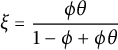 $\displaystyle {\xi =\frac {\phi \theta }{1-\phi +\phi \theta }}$
and
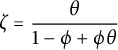 $\displaystyle {\zeta =\frac {\theta }{1-\phi +\phi \theta }}$
.
In order to make the presentation below more concise, we introduce the following terminology.
Definition 3.3 A family of quasi-Banach spaces
 $(A_{p,\gamma })_{p,\gamma \in (0,\infty ]}$
is said to form a real interpolation scale on an interval
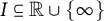 $I \subseteq \mathbb {R}\cup \{\infty \}$
if for every
 $p,q \in I$
,
 $0<\gamma _1,\gamma _2,\gamma \leq \infty $
,
 $0<\theta <1$
, and
 $1/r=(1-\theta )p + \theta /q$
,
 $$ \begin{align*} A_{r, \gamma}= (A_{p,\gamma_1}, A_{q,\gamma_2})_{\theta,\gamma} \end{align*} $$
with equivalent quasi-norms.
The next result may be viewed as a version of Wolff’s interpolation theorem at the level of family of real interpolation scale.
Lemma 3.4 Assume that a family of quasi-Banach spaces
 $(A_{p,\gamma })_{p,\gamma \in (0,\infty ]}$
forms a real interpolation scale on two different intervals
 $I $
and J. If
 $|J \cap I |>1$
, then
 $(A_{p,\gamma })_{p,\gamma \in (0,\infty ]}$
forms a real interpolation scale on
 $I\cup J$
.
Proof We may assume that I and J are closed intervals. As
 $|I\cap J|>1$
, we may assume that
 $\mathrm {sup} I>\inf J $
and
 $I\cap J=[w_1, w_2]$
where
 $w_1=\inf J$
and
 $w_2=\mathrm {sup} I$
. Fix
 $p \in I \setminus J$
,
 $q \in J\setminus I$
, and
 $0<\gamma _1,\gamma _2,\gamma \leq \infty $
. We divide the proof into three cases.
 $\diamond $
Case 1. Assume that
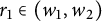 $r_1 \in (w_1, w_2)$
.
Since both p and
 $w_2$
belong to I, by assumption, for any given
 $0<\gamma _3\leq \infty $
,
 $$ \begin{align*} A_{r_1,\gamma}=( A_{p,\gamma_1}, A_{w_2,\gamma_3})_{\theta_1, \gamma}, \end{align*} $$
where
 $1/{r_1}=(1-\theta _1)/p +\theta _1/{w_2}$
.
On the other hand, as
 $r_1$
and q belong to J and
 $r_1<w_2<q$
, the assumption also gives that
 $$ \begin{align*} A_{w_2,\gamma_3} =(A_{r_1,\gamma}, A_{q,\gamma_2})_{\psi_1, \gamma_3} \end{align*} $$
where
 $1/{w_2}= (1-\psi _1)/r_1 + \psi _1/q$
. Applying Wolff’s interpolation theorem, with
 $B_1= A_{p,\gamma _1}$
,
 $B_2=A_{r_1,\gamma }$
,
 $B_3=A_{w_2,\gamma _3}$
, and
 $B_4=A_{q,\gamma _2}$
, we deduce that
 $$ \begin{align*} A_{r_1, \gamma}= (A_{p,\gamma_1}, A_{q,\gamma_2})_{\theta, \gamma}, \end{align*} $$
where
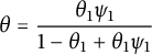 $\displaystyle {\theta =\frac {\theta _1\psi _1}{1-\theta _1 +\theta _1\psi _1}}$
. One can readily verify that
 $1/r_1=(1-\theta )/p +\theta /q$
.
 $\diamond $
Case 2. Assume that
 $r_2 \in (p, w_1]$
.
Fix
 $w_3 \in (w_1, w_2)$
. Since
 $p<r_2<w_3$
and
 $p , w_3 \in I$
, by assumption, we have for every
 $0<\gamma _3\leq \infty $
,
 $$ \begin{align*} A_{r_2,\gamma}=( A_{p,\gamma_1}, A_{w_3,\gamma_3})_{\theta_2, \gamma}, \end{align*} $$
where
 $1/{r_2}=(1-\theta _2)/p + \theta _2/{w_3}$
. Using the previous case with
 $r_2$
in place of p and
 $w_3$
in place of
 $r_1$
, we have
 $$ \begin{align*} A_{w_3,\gamma_3} =( A_{r_2,\gamma}, A_{q,\gamma_2})_{\psi_2, \gamma_3} \end{align*} $$
with
 $1/w_3=(1-\psi _2)/{r_2} + \psi _2/q$
. Using Wolff’s interpolation theorem with
 $B_1=A_{p,\gamma _1}$
,
 $B_2=A_{r_2,\gamma }$
,
 $B_3=A_{w_3,\gamma _3}$
, and
 $B_4= A_{q,\gamma _2}$
, we obtain that
 $$ \begin{align*} A_{r_2,\gamma}=(A_{p,\gamma_1}, A_{q,\gamma_2})_{\theta,\gamma}, \end{align*} $$
where
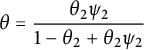 $\displaystyle {\theta =\frac {\theta _2\psi _2}{1-\theta _2 +\theta _2\psi _2}}$
. As before, one can verify that
 $1/{r_2}= (1-\theta )/p + \theta /q$
.
 $\diamond $
Case 3. Assume
 $r_3 \in [w_2, q)$
.
As in the previous case, let
 $w_3 \in (w_1, w_2)$
. Since
 $w_3, r_3, q \in I$
, we have
 $$ \begin{align*} A_{r_3,\gamma}= (A_{w_3, \gamma_3}, A_{q,\gamma_2})_{\theta_3, \gamma}, \end{align*} $$
where
 $1/{r_3}= (1-\theta _3)/{w_3} + \theta _3/q$
. Next, we apply Case 1 with
 $w_3$
in place of
 $r_1$
in order to get that
 $$ \begin{align*} A_{w_3, \gamma_3}= ( A_{p,\gamma_1}, A_{q,\gamma_2})_{\psi_3, \gamma_3} \end{align*} $$
with
 $1/{w_3}=(1-\theta _3)/p +\theta _3/q$
. The desired statement can be deduced as in Case 2.
Combining the three cases above, we may state that if
 $p \in I\setminus J$
,
 $q\in J\setminus I$
,
 $0<\gamma _1,\gamma _2, \gamma \leq \infty $
,
 $0<\theta <1$
, and
 $1/r=(1-\theta )/p +\theta /q$
, then
 $$ \begin{align*} A_{r,\gamma}= (A_{p,\gamma_2}, A_{q,\gamma_2})_{\theta, \gamma}, \end{align*} $$
which is equivalent to the statement that the family
 $(A_{p,\gamma })_{p, \gamma \in (0,\infty ]}$
forms a real interpolation scale on the interval
 $I\cup J$
. ▪
We now state the primary result of the paper. It is an extension of [Reference Bekjan, Chen, Perrin and Yin1, Theorem 4.8] to the full range
 $0<p<\infty $
and a noncommutative generalization of (1.3) (see also [Reference Weisz46]).
Theorem 3.5 If
 $0<\theta <1$
,
 $0<p<\infty $
, and
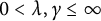 $0<\lambda , \gamma \leq \infty $
, then for
 $1/r=(1-\theta )/p$
,
 $$ \begin{align*} \big( \mathsf{h}_{p,\lambda}^c(\mathcal{M}), \mathsf{bmo}^c(\mathcal{M})\big)_{\theta, \gamma} = \mathsf{h}_{r,\gamma}^c(\mathcal{M}) \end{align*} $$
with equivalent quasi-norms.
Before we proceed, we should point out that for
 $0<p<\infty $
and
 $0<\lambda \leq \infty $
, the pair
 $(\mathsf {h}_{p,\lambda }^c(\mathcal {M}), \mathsf {bmo}^c(\mathcal {M}))$
forms a compatible couple. Indeed, as described in the preliminary section,
 $\mathsf {h}_{p,\lambda }^c(\mathcal {M})$
embeds isometrically into
 $L_{p,\lambda }(\mathcal {M} \overline {\otimes } B(\ell _2(\mathbb {N}^2)))$
which in turn is continuously embedded into the topological vector space
 $L_0(\mathcal {M} \overline {\otimes } B(\ell _2(\mathbb {N}^2)))$
. Now we verify that
 $\mathsf {bmo}^c(\mathcal {M})$
also embeds continuously into
 $L_0(\mathcal {M} \overline {\otimes } B(\ell _2(\mathbb {N}^2)))$
. This is immediate if
 $\mathcal {M}$
is finite as
 $ \mathsf {bmo}^c(\mathcal {M}) \subseteq \mathsf {h}_1^c(\mathcal {M}) \subseteq L_0(\mathcal {M} \overline {\otimes } B(\ell _2(\mathbb {N}^2)))$
. When
 $\mathcal {M}$
is infinite, this can be achieved as follows: since
 $\mathcal {M}_1$
is semifinite, choose a family of mutually disjoint finite projections
 $(e_j)_{j\in J}$
in
 $\mathcal {M}_1$
so that
 $\sum _{j\in J} e_j=\textbf {1}$
for the strong operator topology. Let
 $x=(x_n)_{n\geq 1} \in \mathsf {bmo}^c(\mathcal {M})$
and for each
 $j\in J$
, set
 $xe_j=(x_ne_j)_{n\geq 1}$
. It is clear that
 $xe_j \in \mathsf {bmo}^c(\mathcal {M})$
and
 $s_c^2(xe_j)=e_js_c^2(x) e_j$
. Since
 $\tau (e_j)<\infty $
,
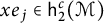 $xe_j \in \mathsf {h}_2^c(\mathcal {M})$
. Therefore
 $U\mathcal {D}_c(x e_j)$
is well-defined in
 $L_0(\mathcal {M} \overline {\otimes } B(\ell _2(\mathbb {N}^2)))$
. Moreover, the module property of U implies that
 $U\mathcal {D}_c(xe_j) =U\mathcal {D}_c(xe_j). (e_j \otimes Id)$
where
 $Id$
is the identity of
 $B(\ell _2(\mathbb {N}^2))$
. This implies that
 $\sum _{j\in J} U\mathcal {D}_c(xe_j)$
converges in measure. This shows in particular that the map
 $x \mapsto \sum _{j\in J} U\mathcal {D}_c(xe_j)$
provides a continuous embedding of
 $\mathsf {bmo}^c(\mathcal {M})$
into
 $L_0(\mathcal {M} \overline {\otimes } B(\ell _2(\mathbb {N}^2)))$
.
Similarly, if
 $0<r,s\leq \infty $
, then
 $ \big ( L_r^{\mathrm {cond}}(\mathcal {M};\ell _2^c), L_s^{\mathrm {cond}}(\mathcal {M};\ell _2^c)\big )$
is a compatible couple as both spaces embed continuously into
 $(L_r+L_s)^{\mathrm {cond}}(\mathcal {M};\ell _2^c)$
.
We need some preparation for the proof. We consider the Orlicz structure of the symmetric function space
 $L_r +tL_s$
for any given
 $0<r<s<\infty $
and
 $t>0$
. To describe this structure, we consider the following Orlicz function:
 $$ \begin{align*} \Phi_t^{(r,s)}(u)=\min\{u^r, t^su^s \} , \quad u\geq 0. \end{align*} $$
One can verify that
 $\Phi _t^{(r,s)}(\cdot )$
is r-convex and s-concave. According to [Reference Hitczenko and Montgomery-Smith15, Lemma 3.2], we have for every
 $f\in L_r +L_s$
and
 $t>0$
,
 $$ \begin{align} 2^{-1-1/r} \big\| f \big\|_{\Phi_t^{(r,s)}} \leq K\big(f, t; L_r, L_s\big) \leq 2 \big\| f \big\|_{\Phi_t^{(r,s)}}. \end{align} $$
In particular, the Orlicz space
 $L_{\Phi _t^{(r,s)}}$
coincides with the space
 $L_r + t L_s$
with isomorphism constant depending only on the index r and therefore independent of t.
Let
 $0<p,q,r,s<2$
and assume that
 $p<q$
,
 $1/p=1/2 +1/r$
, and
 $1/q=1/2 +1/s$
. One can easily check that
 $$ \begin{align*} L_{p} + tL_{q}=L_2 \odot (L_{ r} + tL_{s}). \end{align*} $$
It follows by identification that the following factorization holds for the corresponding Orlicz spaces:
 $$ \begin{align*} L_{\Phi_t^{(p,q)}}= L_2 \odot L_{\Phi_t^{(r,s)}} \end{align*} $$
with constants depending only on the indices p and q.
We will verify that the atomic decomposition results from Theorem 2.8 and Proposition 2.12 apply to this specific factorization. Ideally, we would like to have that the function
 $u\mapsto u^{-1/2}(\Phi _t^{(r,s)})^{-1}(u)$
is equivalent to
 $(\Phi _t^{(p,q)})^{-1}$
but in order to avoid working with inverse functions, we will proceed directly to proving a corresponding result to Lemma 2.4. It also highlights the fact that for this particular case, integral representations of the Orlicz functions involved are not needed. To this end, set for
 $u>0$
,
 $$ \begin{align*} \psi_t^{(p,q)}(u) := (u^{2-p} +t^{-q}u^{2-q})^{-1}. \end{align*} $$
We have the following properties:
Lemma 3.6
-
(i)
$\psi _t^{(p,q)}(u) \approx _{p,q} u^{-2}\Phi _t^{(p,q)}(u)$
; -
(ii)
$\Phi _t^{(r,s)} \big ( (\psi _t^{(p,q)}(u))^{-1/2}\big ) \lesssim _{p,q} \Phi _t^{(p,q)}(u)$
; -
(iii)
$u \mapsto \psi _t^{(p,q)}(u^{1/2})$
is operator monotone decreasing; and -
(iv) for any increasing sequence of positive operators
$a_n\uparrow a$
, we have
$$ \begin{align*} \sum_{n\geq 1} \tau\big( (a_{n+1}^2 -a_n^2)\psi_t^{(p,q)}(a_{n+1})\big) \lesssim_{p,q} \tau\big(\Phi_t^{(p,q)}(a)\big). \end{align*} $$


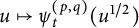


Proof For the first item
 $(i)$
, we write
 $u^{-2}\Phi _t^{(p,q)}(u)=\min \{u^{-2+p}, t^q u^{-2+q}\}=(\max \{u^{2-p}, t^{-q}u^{2-p}\})^{-1}$
and note that
 $$ \begin{align*} 2^{-1}(u^{2-p} + t^{-q}u^{2-p}) \leq \max\{u^{2-p}, t^{-q}u^{2-p} \} \leq u^{2-p} + t^{-q}u^{2-p}. \end{align*} $$
It follows from taking inverses that
 $$ \begin{align*} \psi_t^{(p,q)}(u) \leq u^{-2}\Phi_t^{(p,q)}(u)\leq 2 \psi_t^{(p,q)}(u). \end{align*} $$
Next, item
 $(iii)$
can be seen as follows: if a and b are positive operators with
 $a\leq b$
then since
 $0<1-(p/2) < 1$
and
 $0<1-(q/2)<1$
, we have
 $$ \begin{align*} a^{1-(p/2)} +t^q a^{1-(q/2)} \leq b^{1-(p/2)} +t^q b^{1-(q/2)}. \end{align*} $$
Taking inverse operators, we see that
 $$ \begin{align*} \psi_t^{(p,q)}(b^{1/2}) \leq \psi_t^{(p,q)}(a^{1/2}). \end{align*} $$
This shows that
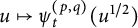 $u\mapsto \psi _t^{(p,q)}(u^{1/2})$
is operator monotone decreasing.
With the equivalence
 $(i)$
on hand, the proof of
 $(iv)$
is identical to the proof of [Reference Randrianantoanina, Wu and Zhou44, Lemma 3.4] so we leave it to the reader. It remains to verify
 $(ii)$
. From the equivalence
 $(i)$
, it suffices to prove that
 $$ \begin{align*} \Phi_t^{(r,s)} \big( u(\Phi_t^{(p,q)}(u))^{-1/2}\big) \lesssim_{p,q} \Phi_t^{(p,q)}(u). \end{align*} $$
Since
 $u(\Phi _t^{(p,q)}(u))^{-1/2}= \max \{u^{1-{p/2}}, t^{-q/2} u^{1-{q/2}}\}$
, we have from the definition of
 $\Phi _t^{(r,s)}(\cdot )$
that
 $$ \begin{align} \Phi_t^{(r,s)} &\big( u(\Phi_t^{(p,q)}(u))^{-1/2}\big)=\nonumber\\ &\min\Big\{\max\{(u^{1-{p/2}})^r, (t^{-q/2} u^{1-{q/2}})^r\}, \max\{t^s(u^{1-{p/2}})^s, t^s(t^{-q/2} u^{1-{q/2}})^s\}\Big\}. \end{align} $$
Note that
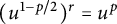 $(u^{1-{p/2}})^r =u^p$
and
 $t^s(t^{-q/2} u^{1-{q/2}})^s=t^qu^q$
. If
 $u^{1-(p/2)} \geq t^{-q/2} u^{1-{q/2}}$
then
 $t^qu^q \geq u^p$
. In particular,
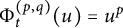 $\Phi _t^{(p,q)}(u)=u^p$
. Then (3.2) implies that
 $$ \begin{align*} \Phi_t^{(r,s)} \big( u(\Phi_t^{(p,q)}(u))^{-1/2}\big)=\min\big\{u^p, t^s (u^{1-(p/2)})^s\big\}\leq \Phi_t^{(p,q)}(u). \end{align*} $$
Similarly, if
 $u^{1-(p/2)} \leq t^{-q/2} u^{1-{q/2}}$
then
 $t^qu^q \leq u^p$
and therefore,
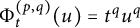 $\Phi _t^{(p,q)}(u)=t^qu^q$
. We can deduce from (3.2) that
 $$ \begin{align*} \Phi_t^{(r,s)} \big( u(\Phi_t^{(p,q)}(u))^{-1/2}\big)=\min\Big\{(t^{-q/2} u^{1-{q/2}})^r, t^q u^q\Big\}\leq \Phi_t^{(p,q)}(u). \end{align*} $$
This completes the proof. ▪
The next proposition constitutes the decisive step toward our proof of Theorem 3.5. We formulate it here for the more general conditioned spaces.
Proposition 3.7 Let
 $\nu $
be a positive integer with
 $\nu \geq 2$
. Assume that
 $2/(\nu +1) <p\leq 2/\nu $
and
 $p <q<2/(\nu -1)$
. If
 $x \in \mathfrak {F}$
, then for every
 $t>0$
,
 $$ \begin{align*} K\big(x,t; L_p^{\mathrm{cond}}(\mathcal{M};\ell_2^c), L_q^{\mathrm{cond}}(\mathcal{M};\ell_2^c)\big) \approx_{p,q} K\big(\sigma_c(x), t; L_p(\mathcal{M}), L_q(\mathcal{M})\big). \end{align*} $$
Proof
 $\bullet $
We observe first that one inequality in the equivalence follows easily from the isometric embeddings described in the preliminary section. Indeed, let
 $x \in \mathfrak {F}$
and set
 $\mathcal {N}= \mathcal {M} \overline {\otimes } B(\ell _2(\mathbb N^2))$
. Recall that for
 $0<r\leq \infty $
, the map
 $U: L_r^{\mathrm {cond}}(\mathcal {M};\ell _2^c) \to L_r(\mathcal {N})$
is an isometry satisfying the identity
 $$ \begin{align*} |U(x)| = \sigma_c(x) \otimes e_{1,1} \otimes e_{1,1}. \end{align*} $$
It follows that for every
 $t>0$
,
 $$ \begin{align*} K\big(\sigma_c(x), t; L_p(\mathcal{M}), L_q(\mathcal{M})\big) &=K\big(|U(x)|, t; L_p(\mathcal{N}), L_q(\mathcal{N})\big)\\ &= K\big(U(x), t; L_p(\mathcal{N}), L_q(\mathcal{N})\big) \\ &\leq K\big(x,t; L_p^{\mathrm{cond}}(\mathcal{M};\ell_2^c), L_q^{\mathrm{cond}}(\mathcal{M};\ell_2^c)\big), \end{align*} $$
which verifies one inequality with constant
 $1$
.
 $\bullet $
The reverse inequality is more involved. We consider the following two finite sequences of indices: set
 $p_0=p$
and
 $q_0=q$
and for
 $1\leq m \leq \nu -1$
,
 $$ \begin{align*} 1/p_{m-1}=1/2 + 1/p_m \ \text{and}\ 1/q_{m-1} =1/2 + 1/q_m. \end{align*} $$
From earlier discussions, the following factorization holds for the respective Orlicz spaces:
 $$ \begin{align*} L_{\Phi_t^{(p_{m-1},q_{m-1})}}= L_2 \odot L_{\Phi_t^{(p_m,q_m)}}. \end{align*} $$
We note that by Lemma 3.6, atomic decompositions stated in Theorem 2.8 and Proposition 2.12 apply to each of these factorizations.
The main idea in the argument below is to repeatedly apply the above factorization until one gets indices that are strictly larger than
 $1$
. At that point, splittings into adapted sequences are possible via the noncommutative Stein inequality. The restriction imposed on the values of p and q is needed in the argument since at every step (except the last one) we need both indices
 $p_m$
and
 $q_m$
to remain in the open interval
 $(0\, ,\, 2)$
so that algebraic atomic decompositions from the previous section can be applied.
We now present the details of the proof. Assume first that
 $x\in \mathfrak {F}^0$
(the general case will be dealt later).
Fix
 $t>0$
. We apply Theorem 2.8 to the Orlicz space
 $L_{\Phi _t^{(p,q)}}$
. We have the following factorization:
 $$ \begin{align} x=\alpha^{(1)}. \, \beta^{(1)}, \end{align} $$
where
 $\alpha ^{(1)}$
is a strictly lower triangular matrix with entries in
 $L_2(\mathcal {M})$
and
 $\beta ^{(1)}$
is an adapted column matrix in
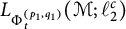 $L_{\Phi _t^{(p_1,q_1)}}(\mathcal {M}; \ell _2^c)$
satisfying:
 $$ \begin{align} \big\|\alpha^{(1)}\big\|_2 . \ \big\|\beta^{(1)} \big\|_{L_{\Phi_t^{(p_1,q_1)}}(\mathcal{M};\ell_2^c)} \lesssim_{p,q} \big\|\sigma_c(x) \big\|_{L_{\Phi_t^{(p,q)}}(\mathcal{M})}. \end{align} $$
Next, we inductively construct finite sequences
 $\{\alpha ^{(m)}: 2\leq m \leq \nu -1 \}$
and
 $\{ \beta ^{(m)} : 1\leq m\leq \nu -1\}$
where the
 $\alpha ^{(m)}$
s are lower triangular matrices taking values in
 $L_2(\mathcal {M})$
satisfying
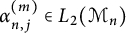 $\alpha ^{(m)}_{n,j} \in L_2(\mathcal {M}_n)$
for
 $1\leq j\leq n$
, and
 $\beta ^{(m)}$
s are adapted column matrices. Both sequences satisfy for
 $2\leq m\leq \nu -1$
:
 $$ \begin{align} \beta^{(m-1)} =\alpha^{(m)}\,. \, \beta^{(m)} \end{align} $$
and
 $$ \begin{align} \big\|\alpha^{(m)}\big\|_2. \ \big\|\beta^{(m)} \big\|_{L_{\Phi_t^{(p_m,q_m)}}(\mathcal{M};\ell_2^c)} \lesssim_{p,q} \big\| \beta^{(m-1)} \big\|_{L_{\Phi_t^{(p_{m-1},q_{m-1})}}(\mathcal{M}; \ell_2^c)}. \end{align} $$
This is done by applying Proposition 2.12 to
 $\beta ^{(m-1)} \in L_{\Phi _t^{(p_{m-1},q_{m-1})}}^{\mathrm {ad}}(\mathcal {M}; \ell _2^c)$
. The constant depends on
 $p_{m-1}$
and
 $q_{m-1}$
but since they depend on p and q respectively, we may state that for each step, the constant depends on p and q.
Clearly, the above construction induces a factorization:
 $$ \begin{align*} x=\alpha^{(1)}\cdots \alpha^{(\nu-1)}\,. \, \beta^{(\nu-1)}. \end{align*} $$
Now, we consider the adapted sequence
 $\beta ^{(\nu -1)}\in L_{\Phi _t^{(p_{\nu -1}, q_{\nu -1})}}(\mathcal {M};\ell _2^c)$
. By identification, we have
 $\beta ^{(\nu -1)} \in (L_{p_{\nu -1}} +t L_{q_{\nu -1}})(\mathcal {M};\ell _2^c)=L_{p_{\nu -1}}(\mathcal {M};\ell _2^c) + t L_{q_{\nu -1}}(\mathcal {M};\ell _2^c)$
.
It follows from the definition of sum of two Banach spaces that
 $\beta ^{(\nu -1)}$
admits a decomposition
 $\beta ^{(\nu -1)}=\xi ^{(1)} +\xi ^{(2)}$
with
 $\xi ^{(1)} \in L_{p_{\nu -1}}(\mathcal {M};\ell _2^c)$
and
 $ \xi ^{(2)} \in L_{q_{\nu -1}}(\mathcal {M};\ell _2^c)$
satisfying the norm estimate:
 $$ \begin{align} \big\| \xi^{(1)} \big\|_{L_{p_{\nu-1}}(\mathcal{M};\ell_2^c)} +t\big\| \xi^{(2)} \big\|_{L_{q_{\nu-1}}(\mathcal{M};\ell_2^c)} \leq 2\big\|\beta^{(\nu-1)} \big\|_{(L_{p_{\nu-1}} + tL_{q_{\nu-1}})(\mathcal{M};\ell_2^c)}. \end{align} $$
The important fact here is that
 $1<p_{\nu -1} <q_{\nu -1} <\infty $
. By applying the noncommutative Stein inequality [Reference Pisier and Xu37], we may replace
 $\xi ^{(1)}$
and
 $\xi ^{(2)}$
by adapted sequences
 $\zeta ^{(1)}=\{\mathcal {E}_n(\xi _n^{(1)})\}_{n\geq 1}$
and
 $\zeta ^{(2)}=\{\mathcal {E}_n(\xi _n^{(2)})\}_{n\geq 1}$
satisfying:
 $$ \begin{align} \big\| \zeta^{(1)} \big\|_{L_{p_{\nu-1}}(\mathcal{M};\ell_2^c)} +t\big\| \zeta^{(2)} \big\|_{L_{q_{\nu-1}}(\mathcal{M};\ell_2^c)} \leq C_{p,q}\big\|\beta^{(\nu-1)} \big\|_{(L_{p_{\nu-1}} + tL_{q_{\nu-1}})(\mathcal{M};\ell_2^c)}. \end{align} $$
The constant
 $C_{p,q}$
can be taken to be equal to
 $2\max \{\gamma _{p_{\nu -1}}, \gamma _{q_{\nu -1}}\}$
where
 $\gamma _r$
is the constant from the noncommutative Stein inequality for
 $1<r<\infty $
. This justifies that
 $C_{p,q}$
depends only on p and q since
 $p_{\nu -1}$
and
 $q_{\nu -1}$
depend on p and q respectively.
Next, we consider two sequences of operators by setting:
 $$ \begin{align*} x^{(1)} =\alpha^{(1)}\cdots \alpha^{(\nu-1)}.\ \zeta^{(1)} \quad \text{and} \quad x^{(2)} =\alpha^{(1)}\cdots \alpha^{(\nu-1)}. \ \zeta^{(2)}. \end{align*} $$
Since
 $\beta ^{(\nu -1)}= \zeta ^{(1)} +\zeta ^{(2)}$
, we clearly have
 $x =x^{(1)} + x^{(2)}$
. We claim that
 $x^{(1)} \in L_p^{\mathrm {cond}}(\mathcal {M};\ell _2^c)$
and
 $x^{(2)} \in L_q^{\mathrm {cond}}(\mathcal {M};\ell _2^c)$
. Indeed, let
 $y^{(1)}=\alpha ^{(2)}\cdots \alpha ^{(\nu -1)}. \ \zeta ^{(1)}$
and
 $y^{(2)}=\alpha ^{(2)}\cdots \alpha ^{(\nu -1)}. \ \zeta ^{(2)}$
. The fact that
 $\zeta ^{(1)}$
is adapted and the property that
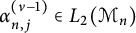 $\alpha _{n,j}^{(\nu -1)} \in L_2(\mathcal {M}_n)$
for
 $1\leq j \leq n$
implies that
 $\widehat {\beta }^{(\nu -2)}:=\alpha ^{(\nu -1)}\,. \, \zeta ^{(1)}$
is an adapted sequence. Moreover, by Hölder’s inequality, we have
 $\widehat {\beta }^{(\nu -2)} \in L_{p_{\nu -2}(\mathcal {M};\ell _2^c)}$
with
 $$ \begin{align*} \big\| \widehat{\beta}^{(\nu-2)}\big\|_{L_{p_{\nu-2}}(\mathcal{M};\ell_2^c)} \leq \big\|\alpha^{(\nu-1)}\big\|_2 \,. \, \big\| \zeta^{(1)} \big\|_{L_{p_{\nu-1}}(\mathcal{M};\ell_2^c)}. \end{align*} $$
One can work backward and set
 $\widehat {\beta }^{(m-1)} = \alpha ^{(m)}\, .\, \widehat {\beta }^{(m)}$
for
 $2\leq m \leq \nu -2$
to see that
 $y^{(1)}$
is an adapted column sequence. Moreover, a repeated use of Hölder’s inequality yields:
 $$ \begin{align*} \big\|y^{(1)}\big\|_{L_{p_1}(\mathcal{M};\ell_2^c)} \leq \left(\prod_{m=2}^{\nu-1} \big\|\alpha^{(m)}\big\|_2\right) \big\| \zeta^{(1)}\big\|_{L_{p_{\nu-1}}(\mathcal{M};\ell_2^c)} <\infty. \end{align*} $$
Since
 $\alpha ^{(1)}$
is strictly lower triangular and
 $y^{(1)}$
is adapted, it follows that
 $x^{(1)}= \alpha ^{(1)}\,. \, y^{(1)} \in L_p^{\mathrm {cond}}(\mathcal {M};\ell _2^c)$
. Similar argument can be applied to deduce that
 $x^{(2)} \in L_q^{\mathrm {cond}}(\mathcal {M};\ell _2^c)$
.
We now verify that the decomposition
 $x= x^{(1)} + x^{(2)}$
provides the desired inequality between the two K-functionals. Indeed, we have the following norm estimates:
 $$ \begin{align*} K\big(x,t; L_p^{\mathrm{cond}}(\mathcal{M};\ell_2^c), &L_q^{\mathrm{cond}}(\mathcal{M};\ell_2^c)\big) \leq \big\|x^{(1)} \big\|_{L_p^{\mathrm{cond}}(\mathcal{M};\ell_2^c)} +t \big\|x^{(2)} \big\|_{L_q^{\mathrm{cond}}(\mathcal{M};\ell_2^c)} \\ &\leq \left(\prod_{m=1}^{\nu-1} \big\|\alpha^{(m)}\big\|_2\right). \big( \big\|\zeta^{(1)}\big\|_{L_{p_{\nu-1}}(\mathcal{M};\ell_2^c)} + t\big\|\zeta^{(2)}\big\|_{L_{q_{\nu-1}}(\mathcal{M};\ell_2^c)} \big)\\ &\lesssim_{p,q}\left( \prod_{m=1}^{\nu-1} \big\|\alpha^{(m)}\big\|_2\right). \, \big\|\beta^{(\nu-1)} \big\|_{(L_{p_{\nu-1}} + tL_{q_{\nu-1}})(\mathcal{M};\ell_2^c)}\\ &\lesssim_{p,q} \left(\prod_{m=1}^{\nu-1} \big\|\alpha^{(m)}\big\|_2 \right). \, \big\|\beta^{(\nu-1)} \big\|_{L_{\Phi_t^{(p_{\nu-1}, q_{\nu-1})}}(\mathcal{M};\ell_2^c)}. \end{align*} $$
Applying (3.6) successively
 $(\nu -2)$
-times, we get
 $$ \begin{align*} K\big(x,t; L_p^{\mathrm{cond}}(\mathcal{M};\ell_2^c), L_q^{\mathrm{cond}}(\mathcal{M};\ell_2^c)\big) \lesssim_{p,q} \big\|\alpha^{(1)}\big\|_2\,. \, \big\|\beta^{(1)} \big\|_{L_{\Phi_t^{(p_{1}, q_{1})}}(\mathcal{M};\ell_2^c)}. \end{align*} $$
By (3.4) and norm equivalence, we arrive at
 $$ \begin{align*} K\big(x,t; L_p^{\mathrm{cond}}(\mathcal{M};\ell_2^c), L_q^{\mathrm{cond}}(\mathcal{M};\ell_2^c)\big) \lesssim_{p,q} \big\| \sigma_c(x) \big\|_{(L_p +tL_q)(\mathcal{M})}. \end{align*} $$
This proves the case where
 $x \in \mathfrak {F}^0$
.
We now consider an arbitrary
 $x=(x_n)_{n\geq 1} \in \mathfrak {F}$
. Let
 $z=(0,x_2, x_3,\dots ) \in \mathfrak {F}^0$
. By the direct sum (2.4) and the previous case, we have:
 $$ \begin{align*} K\big(&x,t; L_p^{\mathrm{cond}}(\mathcal{M};\ell_2^c), L_q^{\mathrm{cond}}(\mathcal{M};\ell_2^c)\big)\\ &\lesssim_{p,q} K\big(x_1, t; L_p^c(\mathcal{M}, \mathcal{E}_1), L_q^c(\mathcal{M},\mathcal{E}_1) \big)+K\big(z,t; L_p^{, \textrm{cond}}(\mathcal{M};\ell_2^c), L_q^{\mathrm{cond}}(\mathcal{M};\ell_2^c)\big)\\ &\lesssim_{p,q} K\big(x_1, t; L_p^c(\mathcal{M},\mathcal{E}_1), L_q^c(\mathcal{M}, \mathcal{E}_1) \big) +K\big(\sigma_c(z), t; L_p(\mathcal{M}), L_q(\mathcal{M}) \big). \end{align*} $$
Since
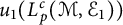 $u_{1}(L_p^c(\mathcal {M},\mathcal {E}_1))$
and
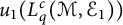 $u_{1}(L_q^c(\mathcal {M},\mathcal {E}_1))$
are one complemented in
 $L_p(\mathcal {M}_1;\ell _2^c)$
and
 $L_q(\mathcal {M}_1;\ell _2^c)$
respectively, we have
 $$ \begin{align*} K\big(x_1, t; L_p^c(\mathcal{M}, \mathcal{E}_1), L_q^c(\mathcal{M},\mathcal{E}_1) \big) &=K\big(u_1(x_1), t; L_p(\mathcal{M}_1; \ell_2^c), L_q(\mathcal{M}_1;\ell_2^c) \big)\\ &=K\big(|u_1(x_1)|, t; L_p(\mathcal{M}_1; \ell_2^c), L_q(\mathcal{M}_1;\ell_2^c) \big). \end{align*} $$
As
 $| u_1(x_1)| =\mathcal {E}_1(|x_1|^2)^{1/2} \otimes e_{1,1}$
, it follows that
 $$ \begin{align*} K\big(x_1, t; L_p^c(\mathcal{M}, \mathcal{E}_1), L_q^c(\mathcal{M},\mathcal{E}_1) \big) = K\big(\mathcal{E}_1(|x_1|^2)^{1/2}, t; L_p(\mathcal{M}_1), L_q(\mathcal{M}_1) \big). \end{align*} $$
As
 $\mathcal {E}_1(|x_1|^2)^{1/2} \leq \sigma _c(x)$
and
 $\sigma _c(z)\leq \sigma _c(x)$
, we may conclude that
 $$ \begin{align*} K\big(x,t; L_p^{\mathrm{cond}}(\mathcal{M};\ell_2^c), L_q^{\mathrm{cond}}(\mathcal{M};\ell_2^c)\big) \lesssim_{p,q} K\big(\sigma_c(x), t; L_p(\mathcal{M}), L_q(\mathcal{M}) \big). \end{align*} $$
The proof is complete. ▪
Using the fact that for every
 $0<r \leq \infty $
,
 $\mathsf {h}_r^c(\mathcal {M})$
embeds isometrically into a one-complemented subspace of
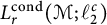 $L_r^{\mathrm {cond}}(\mathcal {M};\ell _2^c)$
, the next result follows immediately from Proposition 3.7.
Corollary 3.8 Let
 $\nu $
be a positive integer with
 $\nu \geq 2$
. Assume that
 $2/(\nu +1) <p\leq 2/\nu $
and
 $p <q< 2/(\nu -1)$
. If y is a finite martingale in
 $\mathfrak {F}(M)$
then for every
 $t>0$
,
 $$ \begin{align*} K\big(y,t; \mathsf{h}_p^c(\mathcal{M}), \mathsf{h}_q^c(\mathcal{M})\big) \approx_{p,q} K\big(s_c(y), t; L_p(\mathcal{M}), L_q(\mathcal{M})\big). \end{align*} $$
Remark 3.9 Since
 $\mathfrak {F}$
is dense in
 $L_p^{\mathrm {cond}}(\mathcal {M};\ell _2^c) +L_q^{\mathrm {cond}}(\mathcal {M};\ell _2^c)$
, we have the following more general assertion that under the assumption of Proposition 3.7, for every
 $x \in L_p^{\mathrm {cond}}(\mathcal {M};\ell _2^c) + L_q^{\mathrm {cond}}(\mathcal {M};\ell _2^c)$
and
 $t>0$
,
 $$ \begin{align*} K\big(x,t; L_p^{\mathrm{cond}}(\mathcal{M};\ell_2^c), L_q^{\mathrm{cond}}(\mathcal{M};\ell_2^c)\big) \approx_{p,q} K\big(U(x) , t; L_p(\mathcal{N}), L_q(\mathcal{N})\big), \end{align*} $$
where
 $\mathcal {N}=\mathcal {M} \overline {\otimes } B(\ell _2(\mathbb N^2))$
.
Similarly, since
 $\mathfrak {F}(M)$
is dense in
 $\mathsf {h}_p^c(\mathcal {M}) + \mathsf {h}_q^c(\mathcal {M})$
, it follows that for every
 $y \in \mathsf {h}_p^c(\mathcal {M}) + \mathsf {h}_q^c(\mathcal {M})$
and
 $t>0$
,
 $$ \begin{align*} K\big(y,t; \mathsf{h}_p^c(\mathcal{M}), h_q^c(\mathcal{M})\big) \approx_{p,q} K\big(U\mathcal{D}_c(y) , t; L_p(\mathcal{N}), L_q(\mathcal{N})\big). \end{align*} $$
3.1 Proof of Theorem 3.5
We consider first two important intermediate cases. One is the Banach space range and the other is when the distance between the two indices is small enough. We begin with the latter.
Lemma 3.10 Let
 $\nu _0 \geq 2$
. Consider
 $2/(\nu _0+1) <p_0 \leq 2/\nu _0$
and
 $p_0<p_1 <2/(\nu _0-1)$
. If
 $0<\theta <1$
,
 $0<\gamma _0,\gamma _1, \gamma \leq \infty $
, and
 $1/r=(1-\theta )/p_0 + \theta /p_1$
, then
 $$ \begin{align*} \mathsf{h}_{r, \gamma}^c(\mathcal{M})= \big( \mathsf{h}_{p_0,\gamma_0}^c(\mathcal{M}) , \mathsf{h}_{p_1,\gamma_1}^c(\mathcal{M})\big)_{\theta, \gamma} \end{align*} $$
with equivalent quasi-norms. ▪
Proof This will be deduced from Corollary 3.8 (see also Remark 3.9) and the description of noncommutative Lorentz spaces as real interpolation of the couple
 $(L_{p_0}(\mathcal {M}), L_{p_1}(\mathcal {M}))$
. Indeed, if
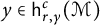 $y \in \mathsf {h}_{r,\gamma }^c(\mathcal {M})$
, then we have:
 $$ \begin{align*} \big\| y \big\|_{\mathsf{h}_{r,\gamma}^c}&=\big\| U\mathcal{D}_c(y)\big\|_{L_{r,\gamma}(\mathcal{N})}\\ &\approx \big\| U\mathcal{D}_c(y)\big\|_{(L_{p_0}(\mathcal{N}), L_{p_1}(\mathcal{N}))_{\theta, \gamma} }\\ &\approx \big\| y \big\|_{(\mathsf{h}_{p_0}^c(\mathcal{M}),\mathsf{h}_{p_1}^c(\mathcal{M}))_{\theta,\gamma}}, \end{align*} $$
where the last equivalence comes from the comparison of K-functionals stated in Remark 3.9. This clearly shows that
 $\mathsf {h}_{r, \gamma }^c(\mathcal {M})= \big ( \mathsf {h}_{p_0}^c(\mathcal {M}) , \mathsf {h}_{p_1}^c(\mathcal {M})\big )_{\theta , \gamma }$
. The full generality as stated in the lemma follows by reiteration. ▪
The next lemma is the infinite version of the Banach space case. It will be deduced from Lemma 3.10 and Wolff’s interpolation theorem. Since our approach differs from [Reference Bekjan, Chen, Perrin and Yin1], we include the details.
Lemma 3.11 Let
 $1<p<r<\infty $
. If
 $1/r=(1-\theta )/p$
then
 $$ \begin{align*} \mathsf{h}_{r, \gamma}^c(\mathcal{M})= \big( \mathsf{h}_p^c(\mathcal{M}) , \mathsf{bmo}^c(\mathcal{M})\big)_{\theta, r} \end{align*} $$
with equivalent norms.
Proof We will verify first that if
 $1<r<q<\infty $
then
 $$ \begin{align} \mathsf{h}_r^c(\mathcal{M})=\big(\mathsf{h}_1^c(\mathcal{M}), \mathsf{h}_q^c(\mathcal{M})\big)_{\psi, r} \end{align} $$
for
 $1/r=(1-\psi ) +\psi /q$
. We separate the proof of (3.9) into three cases:
 $\bullet $
 $1<r<q<2$
. This follows immediately from using
 $\nu _0=2$
,
 $p_0=1$
, and
 $p_1=q$
in Lemma 3.10.
 $\bullet $
 $1<r<2\leq q<\infty $
. Fix v such that
 $1<r<v<2\leq q$
. Applying the previous case, we have
 $$ \begin{align*} \mathsf{h}_r^c(\mathcal{M})=\big(\mathsf{h}_1^c(\mathcal{M}), \mathsf{h}_v^c(\mathcal{M})\big)_{\psi_1, r} \end{align*} $$
for
 $1/r=(1-\psi _1) +\psi _1/v$
. On the other hand, since for every
 $1<s<\infty $
,
 $\mathsf {h}_s^c(\mathcal {M})$
embeds complementably into
 $L_s(\mathcal {M} \overline {\otimes } B(\ell _2(\mathbb {N}^2)))$
, we have for
 $1<r<v< q<\infty $
and
 $1/v= (1-\psi _2)/r + \psi _2/q$
that
 $$ \begin{align*} \mathsf{h}_v^c(\mathcal{M})=\big(\mathsf{h}_r^c(\mathcal{M}), \mathsf{h}_q^c(\mathcal{M})\big)_{\psi_2, v}. \end{align*} $$
Set
 $B_1=\mathsf {h}_1^c(\mathcal {M})$
,
 $B_2=\mathsf {h}_r^c(\mathcal {M})$
,
 $B_3=\mathsf {h}_v^c(\mathcal {M})$
, and
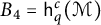 $B_4=\mathsf {h}_q^c(\mathcal {M})$
. It is clear that
 $B_1\cap B_4$
is dense in both
 $B_2$
and
 $B_3$
. Applying Wolff’s interpolation theorem, we deduce (3.9) with
 $\psi =\psi _1\psi _2(1-\psi _2 +\psi _1\psi _2)^{-1}$
. One can easily verify that this is the desired index.
 $\bullet $
 $2\leq r<q<\infty $
. Fix
 $1<u <2 \leq r<q$
and write
 $$ \begin{align*} \mathsf{h}_r^c(\mathcal{M})=\big(\mathsf{h}_u^c(\mathcal{M}), \mathsf{h}_q^c(\mathcal{M})\big)_{\theta_1, r}. \end{align*} $$
Next, we have from the previous case that
 $$ \begin{align*} \mathsf{h}_u^c(\mathcal{M})=\big(\mathsf{h}_1^c(\mathcal{M}), \mathsf{h}_q^c(\mathcal{M})\big)_{\theta_2, u}. \end{align*} $$
Applying Wolff’s interpolation theorem with
 $B_1=\mathsf {h}_1^c(\mathcal {M})$
,
 $B_3=\mathsf {h}_r^c(\mathcal {M})$
,
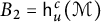 $B_2=\mathsf {h}_u^c(\mathcal {M})$
, and
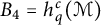 $B_4= h_q^c(\mathcal {M})$
, the desired interpolation follows with
 $\psi = \theta _1(1-\theta _2 +\theta _2\theta _1)^{-1}$
. This proves (3.9).
Using the description of the dual of
 $\mathsf {h}_1^c(\mathcal {M})$
from (2.7) and the well-known fact that
 $(\mathsf {h}_v^c(\mathcal {M}))^*=\mathsf {h}_{v'}^c(\mathcal {M})$
for
 $1<v<\infty $
and
 $v'$
is its conjugate index [Reference Junge and Xu26], we obtain from (3.9) and the duality for interpolation [Reference Bergh and Löfström3, Theorem 3.7.1] that if
 $1<p<r<\infty $
, then
 $$ \begin{align*} \mathsf{h}_r^c(\mathcal{M}) = \big(\mathsf{h}_p^c(\mathcal{M}), \mathsf{bmo}^c(\mathcal{M})\big)_{\theta, r}, \end{align*} $$
which is the desired conclusion. ▪
We are now ready to present the proof of Theorem 3.5. For
 $0<p\leq \infty $
, let
 $A_{p,\gamma } := \mathsf {h}_{p,\gamma }^c(\mathcal {M})$
when
 $0<p<\infty $
and
 $A_{\infty , \gamma }:=\mathsf {bmo}^c(\mathcal {M})$
. Consider the sequence of intervals
 $(I_\nu )_{\nu \geq 1}$
with
 $I_1=(1,\infty ]$
and for
 $\nu \geq 2$
,
 $$ \begin{align*} I_\nu= \bigg(\frac{2}{\nu+1}, \frac{2}{\nu-1}\bigg). \end{align*} $$
For a given
 $ \nu \geq 2$
, it follows from Lemma 3.10 that the family
 $\{ A_{p,\gamma }\}_{p,\gamma \in (0,\infty ]}$
forms a real-interpolation scale on the interval
 $I_\nu $
. On the other hand, by reiteration, Lemma 3.11 gives that the family
 $\{ A_{p,\gamma }\}_{p,\gamma \in (0,\infty ]}$
forms a real-interpolation scale on the interval
 $I_1$
.
Next, we have
 $I_1 \cap I_2= (1,2)$
and for
 $\nu \geq 2$
,
 $I_\nu \cap I_{\nu +1}= (2/(\nu +1), 2/\nu ]$
. By applying Lemma 3.4 inductively, we deduce that the family
 $\{ A_{p,\gamma }\}_{p,\gamma \in (0,\infty ]}$
forms a real-interpolation scale on the interval
 $\bigcup _{\nu =1}^\infty I_\nu = (0,\infty ]$
which is the desired conclusion. ▪
Adapting the argument above by using Proposition 3.7 in place of Corollary 3.8, we also obtain the corresponding result at the level of conditioned spaces.
Proposition 3.12 If
 $0<\theta <1$
,
 $0<p, q<\infty $
, and
 $0<\gamma \leq \infty $
, then for
 $1/{r}=(1-\theta )/{p} + {\theta }/q$
,
 $$ \begin{align*} \big( L_p^{\mathrm{cond}}(\mathcal{M}; \ell_2^c), L_q^{\mathrm{cond}}(\mathcal{M}; \ell_2^c)\big)_{\theta, \gamma} = L_{r,\gamma}^{\mathrm{cond}}(\mathcal{M};\ell_2^c) \end{align*} $$
with equivalent quasi-norms.
3.2 Spaces of adapted sequences
In this subsection, we apply ideas used for the case of conditioned Hardy spaces to the family of spaces of adapted sequences. We first observe that by the noncommutative Stein inequality [Reference Pisier and Xu37], the space of adapted sequences
 $L_p^{\mathrm {ad}}(\mathcal {M};\ell _2^c)$
is complemented in
 $L_p(\mathcal {M};\ell _2^c)$
when
 $1<p<\infty $
. Thus, it is rather an easy task to see that the family
 $\{ L_p^{\mathrm {ad}}(\mathcal {M};\ell _2^c)\}_{1<p<\infty }$
forms interpolation scales. The next result extends this fact to the full range
 $0<p<\infty $
.
Theorem 3.13 If
 $0<\theta <1$
,
 $0<p, q<\infty $
, and
 $0<\gamma \leq \infty $
, then for
 $1/{r}=(1-\theta )/{p} + {\theta }/q$
,
 $$ \begin{align*} \big( L_p^{\mathrm{ad}}(\mathcal{M}; \ell_2^c), L_q^{\mathrm{ad}}(\mathcal{M}; \ell_2^c)\big)_{\theta, \gamma} = L_{r,\gamma}^{\mathrm{ad}}(\mathcal{M};\ell_2^c) \end{align*} $$
with equivalent quasi-norms.
As in the case of conditioned spaces, the proof is based on estimates of K-functionals. We observe first that since
 $L_r(\mathcal {M};\ell _2^c)$
is a one-complemented subspace of
 $L_r(\mathcal {M} \overline {\otimes } B(\ell _2))$
for every
 $0<r<\infty $
, one can easily compute the K-functionals for the couple
 $(L_p(\mathcal {M};\ell _2^c),L_q(\mathcal {M};\ell _2^c))$
. Adapting the argument used in the proof of Proposition 3.7 (using Proposition 2.12 in place of Theorem 2.8 in the first step), we obtain the corresponding result for spaces of adapted sequences. More precisely:
Proposition 3.14 Let
 $\nu $
be a positive integer with
 $\nu \geq 2$
. Assume that
 $2/(\nu +1) <p\leq 2/\nu $
and
 $p <q <2/(\nu -1)$
. For every sequence
 $a \in L_p^{\mathrm {ad}}(\mathcal {M};\ell _2^c)+ L_q^{\mathrm {ad}}(\mathcal {M};\ell _2^c)$
and every
 $t>0$
, the following holds:
 $$ \begin{align*} K\big(a,t; L_p^{\mathrm{ad}}(\mathcal{M};\ell_2^c), L_q^{\mathrm{ad}}(\mathcal{M};\ell_2^c)\big) \approx_{p,q} K\big( \mathcal{S}_c(a), t; L_p(\mathcal{M}), L_q(\mathcal{M})\big). \end{align*} $$
Proof (Sketch of the proof of Theorem 3.13)
First, we use Proposition 3.14 to deduce the corresponding result to Lemma 3.10. Fix
 $\nu _0 \geq 2$
. Assume that
 $2/(\nu _0+1) <p_0 \leq 2/\nu _0$
and
 $p_0<p_1 <2/(\nu _0-1)$
. If
 $0<\theta <1$
,
 $0<\gamma _0,\gamma _1, \gamma \leq \infty $
, and
 $1/r=(1-\theta )/p_0 + \theta /p_1$
, then
 $$ \begin{align} L_{r, \gamma}^{\mathrm{ad}}(\mathcal{M};\ell_2^c)= \big( L_{p_0,\gamma_0}^{\mathrm{ad}}(\mathcal{M};\ell_2^c) , L_{p_1,\gamma_1}^{\mathrm{ad}}(\mathcal{M}; \ell_2^c)\big)_{\theta, \gamma}. \end{align} $$
Next, we deduce the Banach space range using complementation: if
 $1< p<r <q<\infty $
and
 $1/r=(1-\psi )/p + \psi /q$
, then
 $$ \begin{align} L_r^{\mathrm{ad}}(\mathcal{M};\ell_2^c) =\big( L_{p}^{\mathrm{ad}}(\mathcal{M};\ell_2^c) , L_{q}^{\mathrm{ad}}(\mathcal{M}:\ell_2^c)\big)_{\psi, r}. \end{align} $$
Using (3.10) and (3.11), we can repeat the inductive argument used in the proof of Theorem 3.5 with the intervals
 $I_1=(1,\infty )$
and
 $I_\nu =({2}/(\nu +1), {2}/(\nu -1))$
for
 $\nu \geq 2$
, to conclude that the family
 $\{L_p^{\mathrm {ad}}(\mathcal {M};\ell _2^c)\}_{p\in (0, \infty ); \gamma \in (0,\infty ]}$
forms a real interpolation scale. ▪
Assume that
 $1\leq p<\infty $
. We recall that the map
 $\mathcal {D}(x)= (dx_n)_{n\geq 1}$
is an isometric embedding of
 $\mathcal {H}_p^c(\mathcal {M})$
into
 $L_p^{\mathrm {ad}}(\mathcal {M};\ell _2^c)$
. Using the noncommutative Stein inequality when
 $1<p<\infty $
and the noncommutative Lépingle-Yor inequality when
 $p=1$
[Reference Qiu39], the linear map
 $$ \begin{align*} \Pi \big( (a_n)_{n\geq 1}\big)= (a_n-\mathcal{E}_{n-1}(a_n))_{n\geq 1} \end{align*} $$
is simultaneously bounded from
 $L_p^{\mathrm {ad}}(\mathcal {M};\ell _2^c)$
onto
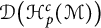 $\mathcal {D}\big (\mathcal {H}_p^c(\mathcal {M})\big )$
for all
 $1\leq p<\infty $
. As a result, one can immediately deduce from Theorem 3.13 that the interpolation
 $$ \begin{align*}(\mathcal{H}_1^c(\mathcal{M}), \mathcal{H}_q^c(\mathcal{M}))_{\theta, r} = \mathcal{H}_r^c(\mathcal{M}) \end{align*} $$
for
 $0<\theta <1$
,
 $1<q<\infty $
, and
 $ 1/r=(1-\theta ) +\theta /q$
holds. Due to this fact, we may view Theorem 3.13 as an extension of the real interpolation version of [Reference Musat32] to the quasi-Banach space range. However, when
 $0<p<1$
, the spaces of adapted sequences cannot be replaced by column martingale Hardy spaces. In fact, only one inclusion holds if column martingale Hardy spaces are used. The next result may be viewed as a noncommutative generalization of [Reference Janson and Jones18, Theorem 2]. We also direct the reader to its companion Corollary 3.19 below and a discussion on the non validity of the reverse inclusions. We refer to [Reference Musat32, Reference Pisier and Xu37] for the definition of
 ${\mathcal {BMO}}^c(\mathcal {M})$
.
Corollary 3.15 Assume that
 $0<p<1$
and
 $0<\theta <\infty $
are such that
 $1/r=(1-\theta )/p <1$
. Then
 $$ \begin{align*} \big( \mathcal{H}_p^c(\mathcal{M}), {\mathcal {BMO}}^c(\mathcal{M}) \big)_{\theta, r}\subset \mathcal{H}_r^c(\mathcal{M}). \end{align*} $$
Proof Let
 $0<\eta <1$
such that
 $1= (1-\eta )/p +\eta /r$
. Let
 $ x\in \big (\mathcal {H}_p^c(\mathcal {M}), \mathcal {H}_r^c(\mathcal {M}) \big )_{\eta , 1}$
. Since
 $\mathcal {H}_u^c(\mathcal {M}) \subset L_u^{\mathrm {ad}}(\mathcal {M};\ell _2^c)$
for
 $u\in \{p,r\}$
, we have
 $$ \begin{align*} \|x\|_{\mathcal{H}_1^c} &=\| dx\|_{L_1^{\mathrm{ad}}(\mathcal{M};\ell_2^c)}\\ &\approx \| dx \|_{(L_p^{\mathrm{ad}}(\mathcal{M};\ell_2^c), L_r^{\mathrm{ad}}(\mathcal{M};\ell_2^c))_{\eta, 1}}\\ &\leq \|x \|_{(\mathcal{H}_p^c(\mathcal{M}), \mathcal{H}_r^c(\mathcal{M}))_{\eta, 1}}, \end{align*} $$
where the second equivalence comes from Proposition 3.13. This shows that
 $$ \begin{align*} \big( \mathcal{H}_p^c(\mathcal{M}), \mathcal{H}_r^c(\mathcal{M}) \big)_{\eta, 1}\subset \mathcal{H}_1^c(\mathcal{M}). \end{align*} $$
Next, we recall that
 $\big (\mathcal {H}_1^c(\mathcal {M}), {\mathcal {BMO}}^c(\mathcal {M})\big )_{\phi , r} =\mathcal {H}_r^c(\mathcal {M})$
where
 $1/r=1-\phi $
. We remark that the Wolff’s interpolation theorem is valid at the level of inclusion: if
 $B_1 \cap B_4 \subset B_2 \cap B_3$
,
 $(B_1, B_3)_{\eta , q_1} \subset B_2$
, and
 $(B_2, B_4)_{\phi , q_2} \subset B_3$
, then
 $(B_1, B_4)_{\theta , q_3} \subset B_3$
whenever
 $0<q_j\leq \infty $
(
 $j=1,2,3$
) and
 $\theta =\phi /(1-\eta +\eta \phi )$
. The verification of this fact can be found in the first part of the proof of [Reference Wolff48, Theorem 1]. Using
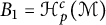 $B_1=\mathcal {H}_p^c(\mathcal {M})$
,
 $B_2=\mathcal {H}_1^c(\mathcal {M})$
,
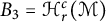 $B_3= \mathcal {H}_r^c(\mathcal {M})$
, and
 $B_4={\mathcal {BMO}}^c(\mathcal {M})$
, we obtain the desired conclusion. ▪
3.3 The complex method
We now turn our attention to the case of complex interpolation method which we now briefly review.
Let S (respectively,
 $\overline {S}$
) denote the open strip
 $\{z : 0< \operatorname {Re} z<1\}$
(respectively, the closed strip
 $\{z : 0\leq \operatorname {Re} z \leq 1\}$
) in the complex plane
 $\mathbb C$
. Let
 $A(S)$
be the collection of
 $\mathbb C$
-valued functions that are analytic on S and continuous and bounded on
 $\overline {S}$
. For a compatible couple of complex quasi-Banach spaces
 $(A_0,A_1)$
, we denote by
 $\mathcal {F}_0(A_0,A_1)$
the family of functions of the form
 $f(z)= \sum _{k=1}^n f_k(z)x_k$
with
 $f_k \in A(S)$
and
 $x_k \in A_0 \cap A_1$
. We equip
 $\mathcal {F}_0(A_0,A_1)$
with the quasi-norm:
 $$ \begin{align*} \big\|f\big\|_{\mathcal{F}_0(A_0,A_1)}= \max \Big\{ \mathop{\mathrm{sup}}_{t\in \mathbb R} \big\| f(it)\big\|_{A_0} , \mathop{\mathrm{sup}}_{t\in \mathbb R} \big\| f(1+it)\big\|_{A_1}\Big\}. \end{align*} $$
Then
 $\mathcal {F}_0(A_0,A_1)$
becomes a quasi-Banach space. For
 $0<\theta <1$
, the complex interpolation norm on
 $A_0 \cap A_1$
is defined by:
 $$ \begin{align*} \big\|x \big\|_{[A_0,A_1]_\theta} =\inf\Big\{\big\|f\big\|_{\mathcal{F}_0(A_0,A_1)} : f(\theta)=x,\ f \in \mathcal{F}_0(A_0,A_1)\Big\}. \end{align*} $$
The complex interpolation space (of exponent
 $\theta $
)
 $[A_0,A_1]_\theta $
is defined as the completion of the quasi-normed space
 $(A_0 \cap A_1, \| \cdot \|_{[A_0,A_1]_\theta })$
.
As in the real method, complex interpolations of the couple
 $(L_p, L_q)$
(for
 $0<p<q\leq \infty $
) are well-known. Indeed, if
 $\mathcal {N}$
is a semifinite von Neumann algebra and
 $0<\theta <1$
, then
 $$ \begin{align*} \big[L_p(\mathcal{N}), L_q(\mathcal{N})\big]_\theta =L_r(\mathcal{N}) \end{align*} $$
isometrically for
 $1/r=(1-\theta )/p +\theta /q$
. This fact comes from [Reference Xu49, Theorem 4.1] (see also [Reference Pisier and Xu38]).
The next result is the version of Theorem 3.5 for the complex method.
Theorem 3.16 If
 $0<p,q<\infty $
,
 $0<\theta <1$
, and
 $ {\frac {1}{r}=\frac {1-\theta }{p} + \frac {\theta }{q}}$
, then
 $$ \begin{align*} \mathsf{h}_r^c(\mathcal{M}) =\big[\mathsf{h}_p^c(\mathcal{M}), \mathsf{h}_q^c(\mathcal{M}) \big]_\theta \end{align*} $$
with equivalent quasi-norms.
For the proof, we will use the next result which provides a connection between complex interpolation method and real interpolation method that is valid for quasi-Banach spaces. We should note that for Banach spaces, the inequality in the next theorem is actually an equivalence but for quasi-Banach spaces only one inequality is valid in its full generality.
Theorem 3.17 [Reference Cwikel, Milman and Sagher9, Theorem 3]
Let
 $(A_0, A_1)$
be a compatible couple of quasi-Banach spaces. Let
 $0<\theta _j<1$
,
 $0<\theta <1$
, and
 $0<\gamma _j\leq \infty $
. Denote
 $E_j= (A_0, A_1)_{\theta _j, \gamma _j}$
for
 $j=0,1$
. If
 $1/\gamma = (1-\theta )/\gamma _0 +\theta /\gamma _1$
and
 $\lambda =(1-\theta )\theta _0 +\theta \theta _1$
then for every
 $a \in A_0\cap A_1\subset E_0 \cap E_1$
,
 $$ \begin{align*} \big\| a \big\|_{[E_0,E_1]_\theta} \leq C \big\|a \big\|_{(A_0, A_1)_{\lambda, \gamma}}. \end{align*} $$
Proof (of Theorem 3.16)
Assume that
 $0<p<q<\infty $
and fix
 $0<p_0<p$
. Then according to Theorem 3.5,
 $\mathsf {h}_p^c(\mathcal {M})=(\mathsf {h}_{p_0}^c(\mathcal {M}), \mathsf {bmo}^c(\mathcal {M}))_{\theta _0, p}$
and
 $h_q^c(\mathcal {M})= (\mathsf {h}_{p_0}^c(\mathcal {M}), \mathsf {bmo}^c(\mathcal {M}))_{\theta _1, q}$
where
 $1/p=(1-\theta _0)/p_0$
and
 $1/q=(1-\theta _1)/p_0$
. We may state from Theorem 3.17 that if
 $1/\gamma = (1-\theta )/p +\theta /q$
and
 $\lambda =(1-\theta )\theta _0 +\theta \theta _1$
then for every
 $a\in \mathsf {h}_{p_0}^c(\mathcal {M}) \cap \mathsf {bmo}^c(\mathcal {M})$
,
 $$ \begin{align*} \big\| a \big\|_{[\mathsf{h}_p^c(\mathcal{M}), \mathsf{h}_q^c(\mathcal{M})]_\theta} \leq C \big\|a\big\|_{(\mathsf{h}_{p_0}^c(\mathcal{M}), \mathsf{bmo}^c(\mathcal{M}))_{\lambda, \gamma}}. \end{align*} $$
One can easily verify that
 $(1-\lambda )/{p_0}=1/\gamma =1/r$
and therefore we may deduce from Theorem 3.5 that
 $$ \begin{align} \big\| a \big\|_{[\mathsf{h}_p^c(\mathcal{M}), \mathsf{h}_q^c(\mathcal{M})]_\theta} \leq C' \big\|a\big\|_{\mathsf{h}_r^c}. \end{align} $$
On the other hand, let
 $U: L_s^{\mathrm {cond}}(\mathcal {M};\ell _2^c) \to L_s(\mathcal N)$
(where
 $\mathcal {N}=\mathcal {M}\overline {\otimes } B(\ell _2(\mathbb {N}^2))$
) be the family of isometric embeddings as described in the preliminary section which are valid for all
 $0<s\leq \infty $
. Denote by
 $\mathcal {D}_c$
the extension of the map
 $x\mapsto (dx_n)_{n\geq 1}$
from
 $\mathsf {h}_s^c(\mathcal {M})$
into
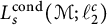 $L_s^{\mathrm {cond}}(\mathcal {M};\ell _2^c)$
. Then for every
 $0<s\leq \infty $
,
 $U\mathcal {D}_c$
is an isometric embedding of
 $\mathsf {h}_s^c(\mathcal {M})$
into
 $L_s(\mathcal {N})$
. Let
 $b \in \mathsf {h}_p^c(\mathcal {M}) \cap \mathsf {h}_q^c(\mathcal {M})$
. Interpolating the operator
 $U\mathcal {D}_c$
, we have
 $$ \begin{align*} \big\| U\mathcal{D}_c(b)\big\|_{[L_p(\mathcal{N}), L_q(\mathcal{N})]_\theta} \leq \big\| b \big\|_{[\mathsf{h}_p^c(\mathcal{M}), \mathsf{h}_q^c(\mathcal{M})]_\theta}. \end{align*} $$
Since
 $\big [(L_p(\mathcal {N}), L_q(\mathcal {N})\big ]_\theta =L_r(\mathcal {N})$
isometrically, it follows that
 $$ \begin{align*} \big\| U\mathcal{D}_c(b)\big\|_{L_r(\mathcal{N})} \leq \big\| b \big\|_{[\mathsf{h}_p^c(\mathcal{M}), \mathsf{h}_q^c(\mathcal{M})]_\theta}. \end{align*} $$
From the fact that
 $U\mathcal {D}_c$
is an isometry on
 $\mathsf {h}_r^c(\mathcal {M})$
, we deduce that
 $$ \begin{align} \big\|b\big\|_{\mathsf{h}_r^c} \leq \big\| b \big\|_{[\mathsf{h}_p^c(\mathcal{M}), \mathsf{h}_q^c(\mathcal{M})]_\theta}. \end{align} $$
From combining (3.12) and (3.13), we obtain the desired equivalence. ▪
When
 $0<p<1$
, we do not know if the corresponding statement to Theorem 3.16 remains valid if the interpolation couple
 $(\mathsf {h}_p^c(\mathcal {M}), \mathsf {bmo}^c(\mathcal {M}))$
is used. Since reiteration theorem is not available for complex interpolations of quasi-Banach spaces, in general, this consideration is independent of Theorem 3.16. We leave this as an open problem.
The same method of proofs can be applied to conditioned spaces and spaces of adapted sequences to deduce the following interpolation results from Proposition 3.12 and Theorem 3.13, respectively.
Proposition 3.18 If
 $0<\theta <1$
and
 $0<p, q<\infty $
then for
 $1/{r}=(1-\theta )/{p} + {\theta }/q$
, the following hold:
 $$ \begin{align*} \big[ L_p^{\mathrm{cond}}(\mathcal{M}; \ell_2^c), L_q^{\mathrm{cond}}(\mathcal{M}; \ell_2^c)\big]_{\theta} = L_{r}^{\mathrm{cond}}(\mathcal{M};\ell_2^c) \end{align*} $$
and
 $$ \begin{align*} \big[ L_p^{\mathrm{ad}}(\mathcal{M}; \ell_2^c), L_q^{\mathrm{ad}}(\mathcal{M}; \ell_2^c)\big]_{\theta} = L_{r}^{\mathrm{ad}}(\mathcal{M};\ell_2^c) \end{align*} $$
with equivalent quasi-norms.
As in the case of real interpolation, we may view the second assertion in the proposition as an extension of Musat’s result to the quasi-Banach space range. Moreover, using [Reference Wolff48, Lemma 1] (which is valid for quasi-Banach spaces), one can adapt the argument used in the proof of Corollary 3.15 to show that the noncommutative analogue of (1.2) holds:
Corollary 3.19 Assume that
 $0<p<1$
and
 $0<\theta <\infty $
are such that
 $1/r=(1-\theta )/p <1$
. Then
 $$ \begin{align*} \big[ \mathcal{H}_p^c(\mathcal{M}), {\mathcal {BMO}}^c(\mathcal{M}) \big]_{\theta}\subset \mathcal{H}_r^c(\mathcal{M}). \end{align*} $$
Our method of proof only applies under the assumption that
 $r>1$
. We should point out that the reverse inclusion does not hold even in the classical setting. An example exhibited in [Reference Janson and Jones18, p. 66] shows that there exists a probability space
 $(\Omega , \mathcal {F},\mathbb {P})$
and an increasing filtration of
 $\sigma $
-fields
 $(\mathcal {F}_n)_{n\geq 1}$
of
 $\mathcal {F}$
with
 $\mathcal {F}=\sigma (\bigcup _{n\geq 1} \mathcal {F}_n)$
and such that if
 $0<p<1<r<\infty $
, then for
 $1/r=(1-\theta )/p$
,
 $\big [ \mathcal {H}_p(\Omega ), {\mathcal {BMO}}(\Omega ) \big ]_{\theta } \neq \mathcal {H}_r(\Omega )$
.
All results stated in this section have row counterparts. However, at the time of this writing, it is unclear if for
 $0<p,q<1$
, the interpolation results for column/row conditioned Hardy spaces have counterparts to the couple of diagonal Hardy spaces
 $(\mathsf {h}_p^d(\mathcal {M}),\mathsf {h}_q^d(\mathcal {M}))$
.
4 Applications to martingale inequalities
In this section, we present various martingale inequalities in the general framework of noncommutative symmetric spaces that can be derived from methods we develop in the previous two sections.
We will need the following generalization of real interpolation:
Definition 4.1 An interpolation space E for a couple of quasi-Banach spaces
 $(E_0,E_1)$
is said to be given by a K-method if there exists a quasi-Banach function space
 $\mathcal {F}$
such that
 $x \in E$
if and only if
 $t\mapsto K(x,t; E_0,E_1) \in \mathcal {F}$
and there exists constant
 $C_E>0$
such that
 $$ \begin{align*} C_E^{-1} \big\| t\mapsto K(x,t; E_0,E_1)\big\|_{\mathcal{F}} \leq \big\|x\big\|_E \leq C_E \big\| t\mapsto K(x,t; E_0,E_1)\big\|_{\mathcal{F}}. \end{align*} $$
In this case, we write
 $E=(E_0, E_1)_{\mathcal {F};K}$
.
Proposition 4.2 Let
 $0<p<q\leq \infty $
. Every interpolation space
 $E\in \mathrm {Int}(L_p,L_q)$
is given by a K-method.
For the Banach space range, this fact is known as a result of Brudnyi and Krugliak (see [Reference Kalton and Montgomery-Smith27, Theorem 6.3]). An argument for the quasi-Banach space range is given in Dirksen’s thesis [Reference Dirksen10]. Alternatively, the quasi-Banach space range can be deduced from the Banach space case as follows: assume that
 $0<p<1$
and
 $E\in \mathrm {Int}(L_p,L_q)$
. Let
 $E^{(1/p)}$
be the
 $1/p$
-convexification of E. That is,
 $$ \begin{align*} E^{(1/p)}= \Big\{h\in L_0 : |h|^{1/p} \in E\Big\} \end{align*} $$
equipped with the norm
 $\| h\|_{E^{(1/p)}}=\| \, |h|^{1/p}\, \|_E^p$
. According to [Reference Cadilhac5, Corollary 4.6],
 $E^{(1/p)} \in \mathrm {Int}(L_1, L_{q/p})$
. Let
 $\mathcal {F}$
be a Banach function space so that
 $E^{(1/p)} =(L_1, L_{q/p})_{ \mathcal {F}; K}$
. We make the observation from Homlsted’s formula [Reference Holmstedt16, Theorem 4.1] that if a is a positive function in
 $L_p +L_q$
then:
 $$ \begin{align*} K\big(a, t; L_p, L_q\big) \approx _{p,q}\Big[ K\big( a^p, t^p; L_1, L_{q/p}\big)\Big]^{1/p}. \end{align*} $$
Let
 $x \in E$
. We have
 $$ \begin{align*} \begin{split} \big\|x\big\|_{E}^{p} &= \big\| \, |x|^{p} \, \big\|_{E^{(1/p)}}\\ &\approx_E \big\| t\mapsto K(|x|^p, t; L_1, L_{q/p})\big\|_{\mathcal{F}}\\ &\approx_E \big\| t\mapsto \big[ K(|x|, t^{1/p}; L_p, L_q)\big]^p\big\|_{\mathcal{F}}\\ &\approx_E\big\| t\mapsto K(|x|, t^{1/p}; L_p, L_q)\big\|_{\mathcal{F}^{(p)}}^p. \end{split} \end{align*} $$
Let
 $\mathcal {Z}=\{ f \in L_0: t\mapsto f(t^{1/p}) \in \mathcal {F}^{(p)}\}$
with the quasi-norm
 $\|f\|_{\mathcal Z}=\|t \mapsto f(t^{1/p})\|_{\mathcal {F}^{(p)}}$
. We see now that
 $E= (L_p, L_q)_{\mathcal {Z}; K}$
. ▪
Below, we will also use the J-method version of the interpolation associated with function space which we now briefly describe: for
 $x \in E_0 +E_1$
, we recall that by a representation of x with respect to the couple
 $(E_0, E_1)$
, we mean a measurable function
 $u: (0,\infty ) \to E_0 \cap E_1$
satisfying
 $$ \begin{align*} x =\int_0^\infty u(t)\ \frac{dt}{t}, \end{align*} $$
where the convergence is taken in
 $E_0 +E_1$
. Recall that for
 $y \in E_0\cap E_1$
and
 $t>0$
,
 $$ \begin{align*} J(y, t; E_0,E_1) = \max\{\|y\|_{E_0}; t \|y\|_{E_1}\}. \end{align*} $$
For a given function space
 $\mathcal {F}$
, we define the quasi-norm
 $$ \begin{align*} \|x\|_{(E_0,E_1)_{\mathcal{F};J}}:=\inf\big\{\|t \mapsto J(u(t), t ;E_0,E_1)\|_{\mathcal{F}}\big\}, \end{align*} $$
where the infimum is taken over all representation
 $u(\cdot )$
of x with respect to the couple
 $(E_0, E_1)$
. The interpolation space
 $(E_0,E_1)_{\mathcal {F};J}$
is defined as the collection of all
 $x \in E_0 + E_1$
for which
 $\|x\|_{(E_0,E_1)_{\mathcal {F};J}}<\infty $
. We refer to [Reference Kreĭn, Petunīn and Semënov30] for more on this interpolation method.
From the fact that every interpolation space of the couple
 $(L_p, L_q)$
is given by a K-method, the following can be easily deduced from our results on K-functionals from the previous section:
Proposition 4.3 Let
 $\nu $
be a positive integer with
 $\nu \geq 2$
. Assume that
 $2/(\nu +1) <p\leq 2/\nu $
and
 $ p<q\leq 2/(\nu -1)$
. If
 $E \in \mathrm {Int}(L_p, L_q)$
with
 $E=(L_p,L_q)_{\mathcal {F};K}$
for a quasi Banach function space
 $\mathcal {F}$
then the following hold:
 $$ \begin{align*}\mathsf{h}_E^c(\mathcal{M}) =( \mathsf{h}_p^c(\mathcal{M}), \mathsf{h}_q^c(\mathcal{M})\big)_{\mathcal{F};K}, \end{align*} $$
 $$ \begin{align*} E^{\mathrm{cond}}(\mathcal{M};\ell_2^c) =\big( L_p^{\mathrm{cond}}(\mathcal{M};\ell_2^c), L_q^{\mathrm{cond}}(\mathcal{M};\ell_2^c)\big)_{\mathcal{F};K}, \end{align*} $$
and
 $$ \begin{align*} E^{\mathrm{ad}}(\mathcal{M};\ell_2^c) =\big( L_p^{\mathrm{ad}}(\mathcal{M};\ell_2^c), L_q^{\mathrm{ad}}(\mathcal{M};\ell_2^c)\big)_{\mathcal{F};K}. \end{align*} $$
The first assertion in the preceding observation motivates the following more general question: assume that
 $E_0$
and
 $E_1$
are symmetric quasi-Banach function spaces and
 $E\in \mathrm {Int}(E_0, E_1)$
, does it follow that
 $\mathsf {h}_E^c(\mathcal {M}) \in \mathrm {Int}\big (\mathsf {h}_{E_0}^c(\mathcal {M}), \mathsf {h}_{E_1}^c(\mathcal {M})\big )$
?
Note that if for
 $j\in \{0,1\}$
,
 $E_j \in \mathrm {Int}(L_{p_j}, L_{q_j})$
for some
 $1<p_j,q_j<\infty $
, then one can deduce from Junge’s representation and interpolation that
 $\mathsf {h}_{E_j}^c(\mathcal {M})$
embeds complementably into
 $E_j(\mathcal {M}\overline {\otimes } B(\ell _2(\mathbb {N}^2)))$
. Thus, in this special case, the answer to the above question is clearly positive. Even for the particular case where
 $E_0=L_p$
and
 $E_1=L_q$
, we do not know if the assumptions on p and q in Proposition 4.3 can be removed when
 $0<p<q\leq 1$
. This of course is closely related to asking whether the statement about K-functionals in Proposition 3.7 is valid for any
 $0<p<q \leq 1$
.
Next, we make the observation that a well-known result for convex functions extends to the general setting of p-convex functions for
 $0<p<1$
.
Proposition 4.4 Let
 $0<p<q<\infty $
, and
 $E \in \mathrm {Int}(L_p, L_q)$
. There exists a constant
 $c_E$
such that the following holds: if f, g are functions such that
 $\|g\|_{L_\Phi } \leq \|f\|_{L_\Phi } $
for every function
 $\Phi $
that is p-convex and q-concave, and if
 $f \in E$
, then
 $g\in E$
with
 $$ \begin{align*} \|g\|_E \leq c_E \|f\|_E. \end{align*} $$
Proof Let f and g as in the statement of the proposition. Using the Orlicz space description of
 $L_p +tL_q$
in the previous section, we have from the assumption that
 $$ \begin{align*} K(g ,t; L_p, L_q) \lesssim_{p,q} K(f,t; L_p, L_q), \quad t>0. \end{align*} $$
According to Proposition 4.2, the interpolation space E is given by a K-method. Fix a function space
 $\mathcal {F}$
so that for every
 $h \in E$
,
 $$ \begin{align*} \|h\|_E \approx_{E} \| t \mapsto K(h,t; L_p, L_q)\|_{\mathcal{F}}. \end{align*} $$
We may now deduce from the inequality on K-functionals that
 $$ \begin{align*} \|g\|_E &\approx_{E} \| t \mapsto K(g,t; L_p, L_q)\|_{\mathcal{F}}\\ &\lesssim_E \| t \mapsto K(f,t; L_p, L_q)\|_{\mathcal{F}}\\ &\approx_{E} \| f\|_E. \end{align*} $$
This verifies the desired conclusion. ▪
Our first result in this section is a comparison between conditioned column space and column space for a class of symmetric spaces.
Theorem 4.5 Let
 $0<p<q<2$
and
 $F\in \mathrm {Int}(L_p, L_q)$
. There exists a constant
 $C_F$
such that for any
 $x \in F^{\mathrm {cond}}(\mathcal {M};\ell _2^c)$
, the following holds:
 $$ \begin{align*} \big\| x \big\|_{F(\mathcal{M};\ell_2^c)}\leq C_F \big\| x \big\|_{F^{\mathrm{cond}}(\mathcal{M};\ell_2^c)}. \end{align*} $$
Similarly, if
 $\Phi $
is an Orlicz function that is p-convex and q-concave for
 $0<p<q<2$
then there exists a constant
 $C_{p,q}$
so that for any sequence
 $x=(x_k)_{k\geq 1}$
with
 $\sigma _c(x) \in L_\Phi (\mathcal {M})$
,
 $$ \begin{align*} \tau\big[\Phi\big( \mathcal{S}_c(x) \big)\big] \leq C_{p,q}\tau\big[\Phi\big(\sigma_c(x)\big)\big]. \end{align*} $$
Proof Let
 $\Phi $
be an Orlicz function that is p-convex and q-concave. According to Theorem 2.8, if
 $x=(x_k)_{k\geq 1} $
in
 $\mathfrak {F}$
, the column vector
 $\overline {x}=\sum _{k\geq 1} x_k \otimes e_{k,1}$
admits a factorization
 $\overline {x}=\alpha \,. \, \beta $
where
 $\alpha $
is a strictly lower triangular matrix taking values in
 $L_2(\mathcal {M})$
and
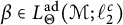 $\beta \in L_{\Theta }^{\mathrm {ad}}(\mathcal {M};\ell _2^c)$
where
 $\Theta $
is the Orlicz function satisfying
 $L_\Phi =L_2 \odot L_\Theta $
(as described in Theorem 2.8) and
 $$ \begin{align*} \big\| \alpha\big\|_{L_2(\mathcal{M} \overline{\otimes} B(\ell_2(\mathbb N)))} . \ \big\|\beta\big\|_{L_\Theta(\mathcal{M};\ell_2^c)} \leq C_{p,q} \big\| x \big\|_{L_\Phi^{\mathrm{cond}}(\mathcal{M};\ell_2^c)}. \end{align*} $$
From the factorization of
 $L_\Phi $
, it follows that
 $$ \begin{align*} \big\| x \big\|_{L_\Phi(\mathcal{M};\ell_2^c)} = \big\| x \big\|_{L_\Phi(\mathcal{M} \overline{\otimes} B(\ell_2(\mathbb{N})))} \leq \big\| \alpha\big\|_{L_2(\mathcal{M} \overline{\otimes} B(\ell_2(\mathbb N)))} . \ \big\|\beta\big\|_{L_\Theta(\mathcal{M};\ell_2^c)}. \end{align*} $$
Combining the two inequalities leads to
 $$ \begin{align*} \big\| \mathcal{S}_c(x) \big\|_{L_\Phi(\mathcal{M})} \leq C_{p,q} \big\| \sigma_c(x) \big\|_{L_\Phi(\mathcal{M})}. \end{align*} $$
By density, we may restate this as there is a map
 $J: L_\Phi ^{\mathrm {cond}}(\mathcal {M};\ell _2^c) \to L_\Phi (\mathcal {M};\ell _2^c)$
with
 $J(x)=x $
for
 $x \in \mathfrak {F}$
. For simplicity, we write
 $J(y)=y$
for arbitrary
 $y \in L_\Phi ^{\mathrm {cond}}(\mathcal {M};\ell _2^c)$
.
Now let
 $\xi $
be an element of
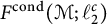 $ F^{\mathrm {cond}}(\mathcal {M}; \ell _2^c)$
. Then, by definition,
 $U(\xi ) \in F(\mathcal {M} \overline {\otimes } B(\ell _2(\mathbb {N}^2)))$
and from boundedness of J implies
 $$ \begin{align*} \big\| \mu( \xi) \big\|_{L_\Phi} \leq C_{p,q} \big\| \mu( U(\xi)) \big\|_{L_\Phi}, \end{align*} $$
where the generalized singular value on the left hand side is taken with respect to
 $\mathcal {M} \overline {\otimes } B(\ell _2(\mathbb {N}))$
and the one the right hand side is taken with respect to
 $\mathcal {M} \overline {\otimes } B(\ell _2(\mathbb {N}^2))$
. It follows from Proposition 4.4 that there exists a constant
 $c_F$
such that
 $$ \begin{align*} \big\| \mu( \xi) \big\|_F \leq C_{F} \big\| \mu( U(\xi)) \big\|_F. \end{align*} $$
This is equivalent to
 $$ \begin{align*} \big\| \xi\big\|_{F(\mathcal{M};\ell_2^c)} \leq C_F \big\| \xi\big\|_{F^{\mathrm{cond}}(\mathcal{M};\ell_2^c)}, \end{align*} $$
which is the desired conclusion.
For the
 $\Phi $
-moment version, it suffices to repeat the above argument but using Remark 2.9 in place of Theorem 2.8. ▪
As an immediate consequence of Theorem 4.5, we have the following extension of the reverse dual Doob inequality proved in [Reference Junge and Xu26, Theorem 7.1] for noncommutative
 $L_p$
spaces (
 $0<p<1$
) to the general case of noncommutative symmetric quasi-Banach spaces.
Corollary 4.6 Let E be a symmetric quasi-Banach function space with
 $E\in \mathrm {Int}(L_p,L_q)$
for
 $0<p<q<1$
. There exists a constant
 $C_E$
so that for any sequence of positive operators
 $(a_k)$
in
 $\mathfrak {F}$
, the following holds:
 $$ \begin{align*} \Big\| \sum_{k\geq 1} a_k \Big\|_{E(\mathcal{M})} \leq C_E \Big\| \sum_{k\geq 1} \mathcal{E}_k(a_k)\Big\|_{E(\mathcal{M})}. \end{align*} $$
Similarly, if
 $\Phi $
is an Orlicz space that is p-convex and q-concave for
 $0<p<q<1$
, then there exists a constant
 $C_{p,q}$
so that for any sequence of positive operators
 $(a_k)$
in
 $\mathfrak {F}$
, the following holds:
 $$ \begin{align*} \tau\left[ \Phi\left(\sum_{k\geq 1} a_k\right) \right] \leq C_{p,q} \tau\left[\Phi\left( \sum_{k\geq 1} \mathcal{E}_k(a_k)\right)\right] \end{align*} $$
Proof Let
 $E\in \mathrm {Int}(L_p, L_q)$
with
 $0<p<q<1$
. Let
 $(a_k)_{k\geq 1}$
be a sequence of positive operators in
 $\mathfrak {F}$
. If
 $E^{(2)}$
is the two-convexification of E, then
 $E^{(2)}\in \mathrm {Int}(L_{2p}, L_{2q})$
. The conclusion follows immediately from the first inequality in Theorem 4.5 using
 $F=E^{(2)}$
and
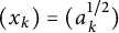 $(x_k)=(a_k^{1/2})$
. Similar argument applies to the
 $\Phi $
-moment case using the second inequality in Theorem 4.5 to the Orlicz function
 $t\mapsto \Phi (t^2)$
. ▪
The next result extends [Reference Jiao, Randrianantoanina, Wu and Zhou20, Theorem 4.11] to the case of noncommutative martingale Hardy spaces associated with symmetric function spaces and moment inequalities.
Theorem 4.7 Let
 $0<p<q<2$
. If
 $F\in \mathrm {Int}(L_p, L_q)$
then there exists a constant
 $C_F$
such that for every
 $x \in \mathsf {h}_F^c(\mathcal {M})$
, the following two inequalities hold:
 $$ \begin{align*} \big\|x\big\|_{\mathcal{H}_F^c(\mathcal{M})} \leq C_F \big\|x\big\|_{\mathsf{h}_F^c(\mathcal{M})} \end{align*} $$
and
 $$ \begin{align*} \big\|x\big\|_{F(\mathcal{M})} \leq C_F \big\|x\big\|_{\mathsf{h}_F^c(\mathcal{M})}. \end{align*} $$
Similarly, if
 $\Phi $
is p-convex and q-concave for
 $0<p<q<2$
then there exists a constant
 $C_{p,q}$
so that for every
 $x\in \mathsf {h}_\Phi ^c(\mathcal {M})$
, we have
 $$ \begin{align*} \max\Big\{ \tau\big[ \Phi\big(S_c(x)\big)\big]; \tau\big[ \Phi\big(|x|\big)\big] \Big\} \leq C_{p,q} \tau\big[ \Phi\big(s_c(x)\big)\big]. \end{align*} $$
Proof
 $\bullet $
For the first inequality, let y be a martingale in
 $\mathfrak {F}(M)$
. Repeating the argument in the proof of Theorem 4.5 with the martingale difference sequence
 $(dy_k)$
, we have for every p-convex and q-concave Orlicz function
 $\Phi $
:
 $$ \begin{align*} \big\| y\big\|_{\mathcal{H}_\Phi^c(\mathcal{M})} \leq C_{p,q} \big\|y\big\|_{\mathsf{h}_\Phi^c(\mathcal{M})}. \end{align*} $$
By density, the above inequality shows that there exists a bounded linear map
 $I: \mathsf {h}_\Phi ^c(\mathcal {M}) \to \mathcal {H}_\Phi ^c(\mathcal {M})$
with
 $I(y)=y$
for every
 $y \in \mathfrak {F}(M)$
. For simplicity, for a given
 $x \in \mathsf {h}_\Phi ^c(\mathcal {M})$
, we will denote
 $I(x)$
by x. That is, for
 $x\in \mathsf {h}_\Phi ^c(\mathcal {M})$
we may state:
 $$ \begin{align*} \big\| \mu(S_c(x)) \big\|_{L_\Phi} \leq C_{p,q} \big\| \mu(| U{\mathcal D}_c(x)|)\big\|_{L_\Phi}, \end{align*} $$
where the generalized singular numbers are computed in the appropriate von Neumann algebras. By Proposition 4.4, there exists a constant
 $C_F$
so that whenever
 $ x \in \mathsf {h}_F^c(\mathcal {M})$
, we have
 $\mu (| U{\mathcal D}_c(x)|)\in F$
and
 $$ \begin{align*} \big\| \mu(S_c(x)) \big\|_{F} \leq C_F \big\| \mu(| U{\mathcal D}_c(x)|)\big\|_{F}. \end{align*} $$
This is equivalent to the first inequality:
 $$ \begin{align*} \big\| x\big\|_{\mathcal{H}_F^c(\mathcal{M})} \leq C_F \big\|x \big\|_{\mathsf{h}_F^c(\mathcal{M})}. \end{align*} $$
 $\bullet $
In view of the argument above, it suffices to verify the second inequality for the case of Orlicz function spaces. For this special case, our proof below is modeled after the argument used in [Reference Chen, Randrianantoanina and Xu7, Corollary 3.14] for the case of
 $L_p$
-spaces. Let
 $\Phi $
be a p-convex and q-concave Orlicz function and x be a martingale in
 $\mathfrak {F}(M)$
. By approximation, we assume that for every
 $n\geq 1$
,
 $s_{c,n}(x)$
is invertible with bounded inverse. As above, we denote
 $s_{c,n}(x)$
by
 $s_n$
and we take
 $s_0=0$
.
Let
 $\lambda>0$
. We write
 $x=\sum _{l\geq 1} a_lb_l$
where for every
 $l\geq 1$
, we set:
 $$ \begin{align*} a_l=\sum_{n\geq l} dx_n \Psi(\lambda s_n)(\Psi(\lambda s_l)^{-1} -\Psi(\lambda s_{l-1})^{-1})^{1/2} \end{align*} $$
and
 $$ \begin{align*} b_l=(\Psi(\lambda s_l)^{-1} -\Psi(\lambda s_{l-1})^{-1})^{1/2}. \end{align*} $$
Using the factorization
 $L_\Phi =L_2 \odot L_\Theta $
, we may deduce that:
 $$ \begin{align*} \big\|x\big\|_{L_\Phi(\mathcal{M})} &= \Big\| \sum_{l\geq 1} a_l b_l\Big\|_{L_\Phi(\mathcal{M})}\\ &\leq \Big\| \left( \sum_{l\geq 1} a_l a_l^*\right)^{1/2} \Big\|_2. \Big\|\left( \sum_{l\geq 1} b_l^* b_l\right)^{1/2}\Big\|_{L_\Theta(\mathcal{M})}\\ &=\left( \sum_{l\geq 1}\big\|a_l\big\|_2^2\right)^{1/2} \big\| \Psi(\lambda s)^{-1/2}\big\|_{L_\Theta(\mathcal{M})}. \end{align*} $$
Following the same reasoning as in the proof of Theorem 2.8, there exists a constant
 $C_{p,q}$
and a corresponding choice of
 $\lambda $
so that
 $$ \begin{align*} \left( \sum_{l\geq 1}\big\|a_l\big\|_2^2\right)^{1/2} \leq C_{p,q} \big\|s_c(x)\big\|_{L_\Phi(\mathcal{M})} \end{align*} $$
and
 $$ \begin{align*} \big\| \Psi(\lambda s)^{-1/2}\big\|_{L_\Theta(\mathcal{M})} \leq 1. \end{align*} $$
This yields that the inequality in the statement is verified for Orlicz function spaces. More precisely,
 $$ \begin{align} \big\|x\big\|_{L_\Phi(\mathcal{M})} \leq C_{p,q} \big\|s_c(x)\big\|_{L_\Phi(\mathcal{M})}. \end{align} $$
The case of moment inequalities follows directly from the moment part of Theorem 4.5 and from using
 $\lambda =1$
in the proof above. ▪
We now proceed with further application of Proposition 2.12. Below, we show that noncommutative Davis decompositions can be easily deduced from factorizations of adapted sequences. We refer to [Reference Junge and Perrin25, Reference Perrin33, Reference Randrianantoanina, Wu and Xu43] for various forms of noncommutative Davis decompositions. We refer to [Reference Randrianantoanina, Wu and Zhou44] for formal definition of the noncommutative vector-valued space
 $L_\Phi (\mathcal {M};\ell _1^c)$
used below.
Theorem 4.8 Assume that
 $0<p<q<2$
and
 $\Phi $
is an Orlicz function that is p-convex and q-concave. Given an adapted sequence
 $\xi =(\xi _n)_{n\geq 1}$
in
 $L_\Phi (\mathcal {M};\ell _2^c)$
, there exist two adapted sequences
 $y=(y_n)_{n\geq 1}$
and
 $z=(z_n)_{n\geq 1}$
such that:
-
(i)
$\xi =y +z$
; -
(ii)
$y \in L_\Phi (\mathcal {M};\ell _1^c)$
with
$\big \| y \big \|_{L_\Phi (\mathcal {M};\ell _1^c)} \lesssim _{p,q} \big \| \xi \|_{L_\Phi (\mathcal {M};\ell _2^c)}$
; and -
(iii)
$z=\lambda a$
where a is an algebraic
$L_\Phi ^{c, \textrm {cond}}$
-atom and
$\lambda \lesssim _{p,q} \big \| \xi \|_{L_\Phi (\mathcal {M};\ell _2^c)}$
.






In particular,
 $$ \begin{align*} \big\| y \big\|_{L_\Phi(\mathcal{M};\ell_1^c)} + \big\| z \big\|_{L_\Phi^{c, \textrm{cond}}(\mathcal{M};\ell_2^c)} \lesssim_{p,q} \big\| \xi \|_{L_\Phi(\mathcal{M};\ell_2^c)}. \end{align*} $$
Proof Let
 $\Theta $
be an Orlicz function such that
 $L_\Phi =L_2 \odot L_\Theta $
. Consider the factorization
 $\xi = \alpha \, .\, \beta $
where
 $\alpha $
is a lower triangular matrix in
 $L_2(\mathcal {M} \overline {\otimes } B(\ell _2(\mathbb N)))$
and
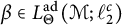 $\beta \in L_\Theta ^{\mathrm {ad}}(\mathcal {M};\ell _2^c)$
according to Proposition 2.12. Define the strictly lower triangular matrix
 $\alpha ^-$
by setting
 $\alpha ^-_{n,j}=\alpha _{n,j}$
for
 $1\leq j <n$
and the diagonal matrix
 $d= \sum _{n\geq 1} \alpha _{n,n} \otimes e_{n,n}$
. Clearly,
 $\alpha = \alpha ^- +d$
. Set:
 $$ \begin{align*} y= d\,. \, \beta \quad\text{and}\quad z= \alpha^-\,. \, \beta. \end{align*} $$
Then
 $\xi =y+z$
and from Proposition 2.12(ii), y and z are adapted. Since
 $\alpha ^-$
is strictly lower triangular and
 $\beta $
is adapted, z is a scalar multiple of an algebraic
 $L_\Phi ^{c, \textrm {cond}}$
-atom. The verification of the norm estimates are straightforward. ▪
We now turn our attention to Davis type inequalities involving other classes of symmetric spaces of measurable operators using interpolation results from the previous section. The next result deals with the case of Lorentz spaces.
Proposition 4.9 Let
 $\xi =(\xi _n)_{n\geq 1}$
be an adapted sequence that belongs to
 $L_{2/3}(\mathcal {M};\ell _2^c)\cap L_2(\mathcal {M};\ell _2^c)$
. Then there exist two adapted sequences
 $y=(y_n)_{n\geq 1}$
and
 $z=(z_n)_{n\geq 1}$
in
 $L_{2/3}(\mathcal {M})\cap L_2( \mathcal {M})$
such that:
-
(i)
$\xi =y +z$
and -
(ii) for every
$2/3<p<2$
and
$0<q\leq \infty $
, the following holds:
$$ \begin{align*} \big\|y\big\|_{L_{p,q}(\mathcal{M} \overline{\otimes}\ell_\infty)} + \big\| z\big\|_{L_{p,q}^{\mathrm{cond}}(\mathcal{M};\ell_2^c)} \lesssim_{p,q}\big\|\xi\big\|_{L_{p,q}(\mathcal{M};\ell_2^c)}. \end{align*} $$


Proof The key ingredients for the proof are the decomposition from [Reference Randrianantoanina, Wu and Xu43, Theorem 3.1] and the two interpolations results from Proposition 3.12 and Theorem 3.13.
Fix
 $\xi \in L_{2/3}^{\mathrm {ad}}(\mathcal {M};\ell _2^c) \cap L_2^{\mathrm {ad}}(\mathcal {M};\ell _2^c)$
. Choose a discrete representation of
 $\xi $
with respect to the couple
 $(L_{2/3}^{\mathrm {ad}}(\mathcal {M};\ell _2^c), L_2^{\mathrm {ad}}(\mathcal {M};\ell _2^c))$
,
 $$ \begin{align*} \xi= \sum_{\nu \in \mathbb Z} \xi^{(\nu)} \end{align*} $$
with
 $\xi ^{(\nu )} \in L_{2/3}^{\mathrm {ad}}(\mathcal {M};\ell _2^c) \cap L_2^{\mathrm {ad}}(\mathcal {M};\ell _2^c)$
for every
 $\nu \in \mathbb Z$
, the series is convergent in
 $L_{2/3}^{\mathrm {ad}}(\mathcal {M};\ell _2^c) + L_2^{\mathrm {ad}}(\mathcal {M};\ell _2^c)$
, and so that
 $$ \begin{align*} J\big( \xi^{(\nu)}, 2^\nu, L_{2/3}^{\mathrm{ad}}(\mathcal{M};\ell_2^c); L_{2}^{\mathrm{ad}}(\mathcal{M};\ell_2^c)\big) \leq 4 K\big( \xi, 2^\nu, L_{2/3}^{\mathrm{ad}}(\mathcal{M};\ell_2^c); L_2^{\mathrm{ad}}(\mathcal{M};\ell_2^c)\big). \end{align*} $$
We refer to [Reference Bergh and Löfström3, Lemma 3.3.2] for the existence of a representation satisfying the properties described above.
For each
 $\nu \in \mathbb {Z}$
, we apply [Reference Randrianantoanina, Wu and Xu43, Theorem 3.1] to the adapted sequence
 $\xi ^{(\nu )}$
: there exists two adapted sequences
 $y^{(\nu )}$
and
 $z^{(\nu )}$
such that
 $\xi ^{(\nu )}=y^{(\nu )} + z^{(\nu )}$
,
 $$ \begin{align*} J\big( y^{(\nu)}, 2^\nu, L_{2/3}(\mathcal{M}\overline{\otimes} \ell_\infty; L_{2}(\mathcal{M}\overline{\otimes} \ell_\infty))\big)\lesssim J\big( \xi^{(\nu)}, 2^\nu, L_{2/3}^{\mathrm{ad}}(\mathcal{M};\ell_2^c); L_2^{\mathrm{ad}}(\mathcal{M};\ell_2^c)\big), \end{align*} $$
and
 $$ \begin{align*} J\big( z^{(\nu)}, 2^\nu, L_{2/3}^{\mathrm{cond}}(\mathcal{M};\ell_2^c); L_2^{\mathrm{cond}}(\mathcal{M};\ell_2^c)\big) \lesssim J\big( \xi^{(\nu)}, 2^\nu, L_{2/3}^{\mathrm{ad}}(\mathcal{M};\ell_2^c); L_2^{\mathrm{ad}}(\mathcal{M};\ell_2^c)\big). \end{align*} $$
It follows that for
 $0<\theta <1$
and
 $0<q\leq \infty $
, we have:
 $$ \begin{align} \big\| (J(y^{(\nu)}, 2^\nu ))_\nu\big\|_{\lambda^{\theta,q}}\lesssim_{\theta,q} \big\| (K(\xi, 2^\nu ))_\nu\big\|_{\lambda^{\theta,q}} \end{align} $$
and
 $$ \begin{align} \big\| (J(z^{(\nu)}, 2^\nu ))_\nu\big\|_{\lambda^{\theta,q}}\lesssim_{\theta,q} \big\| (K(\xi, 2^\nu ))_\nu \big\|_{\lambda^{\theta,q}}, \end{align} $$
where for a given sequence
 $(a_\nu )_{\nu }$
of scalars, we use the quasi-norm
 $$ \begin{align*} \big\| (a_\nu)_{\nu}\big\|_{\lambda^{\theta,q}}:= \Big( \sum_{\nu \in \mathbb Z} \big(2^{-\nu\theta} |a_\nu|\big)^q\Big)^{1/q}. \end{align*} $$
Let
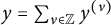 $y= \sum _{\nu \in \mathbb Z} y^{(\nu )}$
and
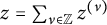 $z=\sum _{\nu \in \mathbb Z} z^{(\nu )}$
. It is clear y and z are adapted sequences and
 $\xi =y+z$
. For any given
 $2/3<p<2$
and
 $0<q\leq \infty $
, choose
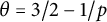 $\theta =3/2-1/p$
. It clearly follows from (4.2) and Theorem 3.13 that:
 $$ \begin{align*} \big\|y \big\|_{L_{p,q}(\mathcal{M}\overline{\otimes} \ell_\infty)} \lesssim_{p,q} \|\xi\|_{L_{p,q}^{\mathrm{ad}}(\mathcal{M};\ell_2^c)}. \end{align*} $$
Similarly, we may deduce from (4.3) and Proposition 3.12 that
 $$ \begin{align*} \big\|z \big\|_{L_{p,q}^{\mathrm{cond}}(\mathcal{M}; \ell_2^c)} \lesssim_{p,q} \|\xi\|_{L_{p,q}^{\mathrm{ad}}(\mathcal{M};\ell_2^c)}. \end{align*} $$
The desired inequality follows from combining the last two inequalities. ▪
We isolate the following important example. Motivated by the noncommutative Khintchine inequality for weak-
 $L_1$
spaces [Reference Cadilhac4], we state below a weak-
 $L_1$
-version of the Davis-decomposition for adapted sequences. This appears to be new even for the classical setting.
Example 4.10 There exists a constant
 $C>0$
so that for every adapted sequence
 $\xi \in L_{1,\infty }(\mathcal {M};\ell _2^c)$
, there exist two adapted sequences y and z such that:
-
(i)
$\xi =x +z$
and -
(ii)
$\big \| y\big \|_{L_{1,\infty }(\mathcal {M} \overline {\otimes } \ell _\infty )} + \big \| z \big \|_{L_{1,\infty }^{\mathrm {cond}}(\mathcal {M}; \ell _2^c)} \leq C \big \| \xi \big \|_{L_{1,\infty }(\mathcal {M};\ell _2^c)}$
.


It is worth pointing out that the preceding example allows us to deduce the noncommutative weak-type
 $(1,1)$
version of the Burkholder/Rosenthal [Reference Randrianantoanina41, Theorem 3.1] from the simpler weak-type inequality involving square functions given in [Reference Randrianantoanina40, Theorem 2.1].
The idea used in the proof of Proposition 4.9 can be extended for the case of general symmetric spaces for the Banach space range. More precisely, we have the following result:
Proposition 4.11 Let E be a Banach function space. If
 $E\in \mathrm {Int}(L_1,L_q)$
for
 $1<q<2$
, then
 $$ \begin{align*} E^{\mathrm{ad}}(\mathcal{M};\ell_2^c) = E(\oplus_{n=1}^\infty \mathcal{M}_n) + E^{\mathrm{cond}, \mathrm{ad}}(\mathcal{M};\ell_2^c), \end{align*} $$
where
 $ E^{\mathrm {cond}, \mathrm {ad}}(\mathcal {M};\ell _2^c)$
denotes is the subspace of
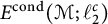 $E^{\mathrm {cond}}(\mathcal {M};\ell _2^c)$
consisting of adapted sequences.
Proof It is easy to see that under the assumption,
 $E(\oplus _{n=1}^\infty \mathcal {M}_n)\subseteq E^{\mathrm {ad}}(\mathcal {M};\ell _2^c) $
. On the other hand, we have from Theorem 4.5 that
 $E^{\mathrm {cond}, \mathrm {ad}}(\mathcal {M};\ell _2^c) \subseteq E^{\mathrm {ad}}(\mathcal {M};\ell _2^c)$
. Thus, we only need to verify one inequality.
The proof rests upon few facts. The interpolation space E is given by a K-method, the simultaneous nature of Proposition 4.9 above, and Proposition 4.3.
Since E is given by a K-method, we may fix a Banach function space
 $\mathcal {F}$
such that for any given semifinite von Neumann algebra
 $\mathcal N$
,
 $$ \begin{align*} C_E^{-1}\big\|a \big\|_{\mathcal{F}; K} \leq \big\|a \big\|_{E(\mathcal N)} \leq \big\|a \big\|_{\mathcal{F}; K}\ , \quad a\in E(\mathcal N). \end{align*} $$
Under the assumption
 $1<q<2$
and Proposition 4.3, we may also state that for every sequence
 $\xi \in E^{\mathrm {ad}}(\mathcal {M};\ell _2^c)$
,
 $$ \begin{align*} \big\| \xi\big\|_{\big(L_1^{\mathrm{ad}}(\mathcal{M};\ell_2^c); L_q^{\mathrm{ad}}(\mathcal{M};\ell_2^c)\big)_{\mathcal{F};K}} \approx_E \big\|\xi\big\|_{E^{\mathrm{ad}}(\mathcal{M};\ell_2^c)}. \end{align*} $$
Similarly, for every
 $\zeta \in E^{\mathrm {cond}}(\mathcal {M};\ell _2^c)$
,
 $$ \begin{align*} \big\| \zeta\big\|_{\big(L_1^{\mathrm{cond}}(\mathcal{M};\ell_2^c); L_q^{\mathrm{cond}}(\mathcal{M};\ell_2^c)\big)_{\mathcal{F};K}} \approx_{E} \big\|\zeta \big\|_{E^{\mathrm{cond}}(\mathcal{M};\ell_2^c)}. \end{align*} $$
We now outline the argument. Fix
 $\xi \in L_1^{\mathrm {ad}}(\mathcal {M};\ell _2^c) \cap L_q^{\mathrm {ad}}(\mathcal {M};\ell _2^c)\big )$
. Repeating the argument in the proof of Proposition 4.9 (taking into account the fact that the decomposition in Proposition 4.9 works simultaneously), we obtain a decomposition
 $\xi =y +z$
where
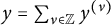 $y=\sum _{\nu \in \mathbb Z} y^{(\nu )}$
and
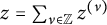 $z=\sum _{\nu \in \mathbb Z} z^{(\nu )}$
are representations with respect to the couple
 $(L_1(\mathcal {M}\overline {\otimes }\ell _\infty ),L_q(\mathcal {M}\overline {\otimes }\ell _\infty ))$
and
 $(L_1^{\mathrm {cond}}(\mathcal {M}; \ell _2^c),L_q^{\mathrm {cond}}(\mathcal {M};\ell _2^c))$
respectively and further satisfy that for every
 $\nu \in \mathbb Z$
,
 $$ \begin{align*} J\big( y^{(\nu)}, 2^\nu, L_1(\mathcal{M}\overline{\otimes}\ell_\infty); L_q(\mathcal{M} \overline{\otimes} \ell_\infty)\big) \lesssim_{q} K\big( \xi, 2^\nu, L_1^{\mathrm{ad}}(\mathcal{M};\ell_2^c); L_q^{\mathrm{ad}}(\mathcal{M};\ell_2^c)\big) \end{align*} $$
and
 $$ \begin{align*} J\big( z^{(\nu)}, 2^\nu, L_1^{\mathrm{cond}}(\mathcal{M};\ell_2^c); L_q^{\mathrm{cond}}(\mathcal{M};\ell_2^c)\big) \lesssim_{q} K\big( \xi, 2^\nu, L_1^{\mathrm{ad}}(\mathcal{M};\ell_2^c); L_q^{\mathrm{ad}}(\mathcal{M};\ell_2^c)\big). \end{align*} $$
Consider the following functions defined on the semi-axis
 $(0,\infty )$
:
 $$ \begin{align*} f(t) = J(y^{(\nu)}, 2^\nu)\quad \text{for} \ t \in [2^\nu, 2^{\nu+1}), \end{align*} $$
 $$ \begin{align*} g(t) = J(z^{(\nu)}, 2^\nu)\quad \text{for} \ t \in [2^\nu, 2^{\nu+1}), \end{align*} $$
and
 $$ \begin{align*} h(t)=K(\xi, 2^\nu)\quad \text{for} \ t \in [2^\nu, 2^{\nu+1}). \end{align*} $$
It follows that for every
 $t>0$
,
 $$ \begin{align*} \max\big\{ f(t); g(t) \big\} \lesssim_{q} h(t). \end{align*} $$
Taking the norms on the function space
 $\mathcal {F}$
, we have
 $$ \begin{align*} \big\|f\big\|_{\mathcal{F}} + \big\|g\big\|_{\mathcal{F}} \lesssim_q \big\|h\big\|_{\mathcal{F}}. \end{align*} $$
From the definitions of the three functions, we further get that:
 $$ \begin{align} \|y\|_{(L_1(\mathcal{M}\overline{\otimes}\ell_\infty), L_q(\mathcal{M}\overline{\otimes}\ell_\infty)_{\mathcal{F};J}} &+ \|z\|_{(L_1^{\mathrm{cond}}(\mathcal{M};\ell_2^c); L_q^{\mathrm{cond}}(\mathcal{M};\ell_2^c))_{\mathcal{F};J}}\nonumber\\ &\lesssim_q \|\xi\|_{(L_1^{\mathrm{ad}}(\mathcal{M};\ell_2^c); L_q^{\mathrm{ad}}(\mathcal{M};\ell_2^c))_{\mathcal{F};K}}. \end{align} $$
From the equivalence of the J-methods and K-methods relative the function space
 $\mathcal {F}$
(see for instance, [Reference Kreĭn, Petunīn and Semënov30, Theorem 2.9]) and the equivalence of norms stated at the beginning of the proof, we may conclude that:
 $$ \begin{align*} \|y\|_{E(\mathcal{M}\overline{\otimes} \ell_\infty)} + \|z\|_{E^{\mathrm{cond}}(\mathcal{M};\ell_2^c)} \lesssim_E \|\xi\|_{E^{\mathrm{ad}}(\mathcal{M};\ell_2^c)}, \end{align*} $$
which is the desired inequality. ▪
Remark 4.12 The argument in the proof of Theorem 4.11 can be carried out for the larger class
 $E\in \mathrm {Int}(L_p, L_q)$
with
 $2/3<p<q<2$
to get that every
 $\xi \in L_{p}^{\mathrm {ad}}(\mathcal {M};\ell _2^c) \cap L_{q}^{\mathrm {ad}}(\mathcal {M};\ell _2^c)$
admits a decomposition into two adapted sequences y and z satisfying:
 $$ \begin{align*} \|y\|_{(L_p(\mathcal{M}\overline{\otimes}\ell_\infty), L_q(\mathcal{M}\overline{\otimes}\ell_\infty)_{\mathcal{F};J}} + \|z\|_{(L_p^{\mathrm{cond}}(\mathcal{M};\ell_2^c); L_q^{\mathrm{cond}}(\mathcal{M};\ell_2^c))_{\mathcal{F};J}} \lesssim_{E} \|\xi\|_{ E^{\mathrm{ad}}(\mathcal{M};\ell_2^c)}. \end{align*} $$
However, we do not know if the equivalence of the J-method and the K-method relative to the function space
 $\mathcal {F}$
is valid for the case of quasi-Banach couples.
As an immediate application of Proposition 4.11, we deduce the next result which partially answers a problem from [Reference Randrianantoanina, Wu and Xu43, Remark 3.11].
Corollary 4.13 Let E be a Banach function space. If
 $E \in \mathrm {Int}(L_1, L_q)$
for
 $1<q<2$
, then
 $$ \begin{align*} \mathcal{H}_E^c(\mathcal{M}) = \mathsf{h}_E^d(\mathcal{M}) + \mathsf{h}_E^c(\mathcal{M}). \end{align*} $$
Proof We only need to verify the inclusion
 $\mathcal {H}_E^c(\mathcal {M}) \subseteq \mathsf {h}_E^d(\mathcal {M}) + \mathsf {h}_E^d(\mathcal {M})$
. That is to show the existence of a constant
 $\alpha _E$
such that for every
 $x \in \mathcal {H}_E^c(\mathcal {M})$
, the following holds:
 $$ \begin{align*} \inf\left\{ \big\|x^d\big\|_{\mathsf{h}_E^d} + \big\|x^c\big\|_{\mathsf{h}_E^c} \right\} \leq \alpha_E \big\|x \big\|_{\mathcal{H}_E^c}, \end{align*} $$
where the infimum is taken over all
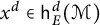 $x^d \in \mathsf {h}_E^d(\mathcal {M})$
and
 $x^c \in \mathsf {h}_E^c(\mathcal {M})$
such that
 $x=x^d + x^c$
.
Let
 $\xi =(dx_n)_{n\geq 1} \in E^{\mathrm {ad}}(\mathcal {M};\ell _2^c)$
. It is enough to take martingales
 $x^c$
and
 $x^d$
with for every
 $n\geq 1$
,
 $$ \begin{align*} dx_n^c= z_n - \mathcal{E}_{n-1}(z_n) \quad \text{and} \quad dx_n^d= y_n - \mathcal{E}_{n-1}(y_n), \end{align*} $$
where y and z are the adapted sequences from Theorem 4.11. Clearly,
 $x=x^d +x^c$
. Since the map
 $(a_n)_{n\geq 1}\mapsto (\mathcal {E}_{n-1}(a_n))_{n\geq 1} $
is a contraction in
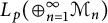 $L_p(\oplus _{n=1}^\infty \mathcal {M}_n)$
for every
 $1\leq p<\infty $
, it follows by interpolation that it is also bounded in
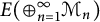 $E(\oplus _{n=1}^\infty \mathcal {M}_n)$
. In particular,
 $$ \begin{align*} \|x^d\|_{\mathsf{h}_E^d} \lesssim_E \|y\|_{E(\oplus_{n=1}^\infty \mathcal{M}_n)}. \end{align*} $$
On the other hand, since for every
 $n\geq 1$
,
 $\mathcal {E}_{n-1}|dx_n^c|^2 \leq \mathcal {E}_{n-1}|z_n|^2$
, we immediately get that
 $$ \begin{align*} \|x^c\|_{\mathsf{h}_E^c} \leq \|z\|_{E^{\mathrm{cond}}(\mathcal{M};\ell_2^c)}. \end{align*} $$
Combining these two inequalities, we arrive at
 $$ \begin{align*} \|x^d\|_{\mathsf{h}_E^d} + \|x^c\|_{\mathsf{h}_E^c} \lesssim_E \|\xi\|_{E^{\mathrm{ad}}(\mathcal{M};\ell_2^c)} =\|x\|_{\mathcal{H}_E^c}. \end{align*} $$
The proof is complete. ▪
We recall that the conclusion of Corollary 4.13 also applies to interpolation space
 $E \in \mathrm {Int}(L_p, L_2)$
for
 $1<p<2$
(see [Reference Randrianantoanina, Wu and Xu43, Theorem 3.9]). We suspect that the preceding corollary is valid for any Banach function space in
 $\mathrm {Int}(L_1, L_2)$
but our method is restricted to
 $1<q<2$
(see also [Reference Randrianantoanina and Wu42, Problem 4.2] for a related question).
As examples of spaces that are not covered by previously known results, we consider the general Lorentz space
 $\Lambda _{1, w}$
where w is a positive decreasing function on
 $(0,\infty )$
with
 $\int _0^\infty w(t)\ dt=\infty $
. The Lorentz space
 $\Lambda _{1,w}$
is the linear space consisting of all
 $ f\in L_0$
such that
 $$ \begin{align*} \big\|f\big\|_{\Lambda_{1,w}} =\int_0^\infty \mu_t(f) w(t)\ dt <\infty. \end{align*} $$
The space
 $(\Lambda _{1,w}, \|\cdot \|_{\Lambda _{1,w}})$
is a fully symmetric Banach function space. According to [Reference Kamińska, Maligranda and Persson29],
 $\Lambda _{1,w}$
is r-concave if and only if (for
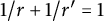 $1/r +1/r'=1$
),
 $$ \begin{align*} \left( \frac{1}{t} \int_0^t w(s)^{r'} \ ds \right)^{1/r'} \lesssim w(t), \quad t>0. \end{align*} $$
With the preceding criterion, one can isolate the family of weights w for which
 $\Lambda _{1,w} \in \mathrm {Int}(L_1, L_q)$
for some
 $1<q<2$
and therefore the Davis decomposition applies to martingales from the corresponding Hardy spaces
 $\mathcal {H}_{\Lambda _{1,w}}^c(\mathcal {M})$
.
Acknowledgment
I am grateful to the anonymous referee for a careful reading of the paper and for useful comments which improved the presentation of the paper.



