1. Introduction
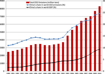
As the main greenhouse gas (GHG), carbon dioxide (CO2) is considered to be the most important cause of global warming. In recent years, due to rapid economic growth, China's CO2 emissions have increased rapidly. According to the estimations of the Carbon Dioxide Information Analysis Center (CDIAC), China's CO2 emissions expanded by more than three-fold within two decades, from 2,461 million tons in 1990 to 8,241 million tons in 2010. Since 2007, China has overtaken the United States as the world's largest CO2 emitter. Moreover, in 2010, China's total CO2 emissions accounted for approximately a quarter of the world's total emissions; emissions from China represented as much as 68 per cent of the total increase in global CO2 emissions between 2000 and 2010 (Nandi Reference Nandi2013). Figure 1 depicts China's CO2 emissions and its share of global emissions since 1990. For comparison, China's share of world GDP in the same period is also included in the figure. From 1990 to 2011, China's share of world GDP rose by 7.8 per cent, from 1.63 to 9.39 per cent, whereas China's CO2 emissions proportion increased by 13.7 per cent, from 10.95 to 24.65 per cent, during the same period.
China's total CO2 emissions (left scale), its share of global emissions (right scale), and its share of world GDP (right scale) since 1990

The fact that China's share of world CO2 emissions grew faster than its share of world GDP partly reflects China's extensive growth during the two decades from 1990 to 2011, which relied heavily on energy consumption and generated increasing levels of pollution.Footnote 1 Because the conventional extensive growth model has brought mounting tensions to resources and the environment, it has proven to be unsustainable and needs to be shifted to a more intensive growth pattern, typically identified with more efficient energy consumption and lower pollution emissions. Meanwhile, international pressure to shift the pattern of growth has also increased, in terms of pressure to control GHG emissions and mitigate global warming. Given China's remarkable share of global CO2 emissions and its rapid growth (see figure 1), the international community's concern over China's CO2 emissions is increasing.
Despite the necessity of controlling CO2 emissions and the Chinese government's commitment to do so, there is a vigorous debate within academic circles and the international community at large about how rapidly CO2 emissions in China could be reduced, if at all.Footnote 2 Given China's high volume of CO2 emissions and its current growth trend, the key questions of concern for the international community and academics include: when will the turning point in China's CO2 emissions occur, if at all? If there is a turning point, how high will the emission peak be? Additionally, and more importantly, under what circumstances will the turning point exist? Will it occur as a natural outcome of China's economic development or as a consequence of government intervention? In order to answer these questions convincingly, the theory of the CO2 environmental Kuznets curve (CKC) is utilized and examined herein. Literally speaking, CKC is a special case of the environmental Kuznets curve (EKC), which was first introduced by Grossman and Kruger (Reference Grossman and Kruger1991) to describe a hypothesized U-shaped relationship between various indicators of environmental degradation and income per capita: in the early stage of economic development, pollution increases and the environment deteriorates; however, beyond a certain level of income per capita, pollution decreases and the environment improves.
As stressed in survey papers such as Stern (Reference Stern2004) and Dinda (Reference Dinda2004), the existing empirical EKC literature contains problems in both empirical and theoretical aspects. In the empirical aspect, it is already well known that the empirical results from EKC analyses (including the positions of the turning points of the studied pollutants) are highly sensitive to the regression specifications, the variables used as the regressors, and even the sample size. The differences in empirical results from EKC analyses are so large that there has as yet been no consensus regarding whether the EKC relationship is valid. For instance, although the empirical studies of Cole et al. (Reference Cole, Rayner and Bates1997), Schmalensee et al. (Reference Schmalensee, Stoker and Judson1998), Galeotti and Lanza (Reference Galeotti and Lanza2005) and Auffhammer and Carson (Reference Auffhammer and Carson2008) support the existence of a CKC,, Roca and Alcántara Reference Roca and Alcántara2001, Azomahou et al. (Reference Azomahou, Laisney and Nguyen Van2006) and He and Richard (Reference He and Richard2009) all claim that the empirical results do not favor the existence of a turning point in CO2 emissions. Torras and Boyce (Reference Torras and Boyce1998) verify that the emission peak only exists for certain types of pollutants. Galeotti et al. (Reference Galeotti, Lanza and Pauli2006) find evidence supporting the existence of a CKC only in OECD nations. Some studies have even reported that the relationship between pollutants and income follows various shapes such as a ‘U’, ‘inverted-U’, ‘N’ or ‘inverted-N’ (e.g., Holtz-Eakin and Selden Reference Holtz-Eakin and Selden1995; Moomaw and Unruh Reference Moomaw and Unruh1997; Torras and Boyce Reference Torras and Boyce1998; Duarte et al. Reference Duarte, Pinilla and Serrano2013). Moreover, as Wagner (Reference Wagner2008) noted, nearly all these empirical studies on CKC are subject to several major econometric complications such as ignoring the nonlinear transformations of integrated regressors and the cross-sectional dependence in the panel context. In a recent study, Itkonen (Reference Itkonen2012) claims that recent studies estimating the CKC by adding energy consumption as a control variable are subject to model misspecifications related to the econometric methodology and data definition used. On the theoretical side, a growing body of literature has emerged to provide theoretical explanations for the inverted-U shaped EKC, including Stokey (Reference Stokey1998), Andreoni and Levinson (Reference Andreoni and Levinson2001) and Brock and Taylor (Reference Brock, Taylor, Aghion and Durlauf2005); Brock and Taylor Reference Brock and Taylor2010. However, very few of these theoretical explanations can be used to guide empirical estimations directly. The empirical EKC/CKC literature to date has basically examined the EKC/CKC as a purely empirical relationship, which is also one important reason why different empirical studies vary considerably in their forms of estimation and their results. The latest development in EKC/CKC estimations involves utilizing more advanced methodologies and/or specific regression specifications. Some representative studies include: Azomahou et al. (Reference Azomahou, Laisney and Nguyen Van2006) and Nguyen-Van (Reference Nguyen-Van2010), which utilized nonparametric and semiparametric panel data analyses to investigate the EKC for CO2 emissions and energy consumption, respectively; Fouquau et al. (Reference Fouquau, Destais and Hurlin2009), which used a threshold panel specification to estimate EKC for energy demand; Duarte et al. (Reference Duarte, Pinilla and Serrano2013), which employed a panel smooth transition approach to examine EKC for water use; and Jobert et al. (Reference Jobert, Karanfil and Tykhonenko2014), which applied a Bayesian shrinkage approach to estimate a country-specific EKC from panel data. However, although the utilization of new methodologies could improve the quality of estimations to some extent, some fundamental problems involved with the EKC framework, as Stern (Reference Stern2004) and Dinda (Reference Dinda2004) claim, still exist.
Given the potential problems and flaws in EKC estimation and other empirical forecasting models, we refrain from making forecasts on the basis of empirical frameworks in this study.Footnote 3 Instead, our forecast is conducted utilizing the ‘Green Solow model’ (GSM) as the main theoretical tool. Developed by Brock and Taylor (Reference Brock and Taylor2010), the GSM is a neoclassical theoretical framework that incorporates pollutant emissions into the textbook Solow model. Under the GSM framework, the projection of China's CO2 emissions can be completely determined when some key parameters in the model are fixed. The inverted-U shaped CKC can be observed if certain conditions of the key parameters are met. Concretely speaking, the contribution of this paper is two-fold. First, the prediction of the GSM that there would exist convergence in per capita CO2 emissions across Chinese provinces is verified with China's provincial panel data. The convergence not only confirms the applicability of GSM to China but also implies that China's provincial CO2 emissions tend to stabilize, which is a necessary condition for the existence of a turning point in China's total CO2 emissions in the long run. Although some studies have found evidence supporting the convergence of some pollutants, including CO2, across countries (Chang and Lee Reference Chang and Lee2008; Ordás Criado et al. Reference Ordás Criado, Valente and Stengos2011), this study represents the first time that the convergence in per capita CO2 emissions across Chinese provinces is verified. Secondly, using reasonable values for the GSM's key parameters for the three regions of China (eastern, central and western), the projections of China's CO2 emissions between 2011 and 2080 are forecast based on the predictions for the three regions with the GSM framework.Footnote 4 The results indicate that China's total CO2 emissions would peak approximately in the year 2041 in the benchmark scenario.
The rest of this paper proceeds as follows. In section 2, the framework of the GSM and its relationship to the EKC are briefly introduced. In section 3, an empirical study is conducted to examine a key prediction of the GSM, that there is a convergence in per capita CO2 emissions across Chinese provinces. In section 4, after the values of the key parameters of the EKC are determined for the three regions, the trajectories of CO2 emissions for these regions and the country as a whole are forecast. Some international comparisons are also implemented to check the reasonableness of the forecast results. Finally, section 5 concludes and suggests directions for further studies.
2. The Green Solow model
The GSM was originally developed by Brock and Taylor (Reference Brock and Taylor2010). As the model's name reveals, the GSM includes the basic elements of the textbook Solow model developed by Solow (Reference Solow1956). The only differences in the GSM are the introduction of CO2 emissions as an unwanted by-product and exogenous technology progress in pollution abatement.Footnote 5 The core equations that describe the dynamics of capital stock and pollutant emissions are:
 $$\displaystyle{{\dot{k}} \over {k}} = \lpar 1-\theta\rpar sk^{\alpha -1}-\lpar \delta+n+g_B\rpar $$
 $$\displaystyle{{e_C} \over {e_C}} = \left(g_B +\alpha \displaystyle {{k^{\prime\prime}} \over {k}} \right)-\hbox{g}_A $$
 $$\displaystyle{{\dot{E}} \over {E}} = \left(n+g_B +\alpha \displaystyle{{\dot{k}} \over {k}} \right)-\hbox{g}_A $$
where k denotes the capital stock per effective worker, e
C
represents the pollution emissions per capita, and E represents total CO2 emissions. The variables s, δ, n, g
B
and g
A
represent saving rate, depreciation rate, population growth rate, productive technology growth rate and the growth rate for carbon efficiency, respectively. The variable α is the production elasticity of capital stock, and θ is the ratio of investment in CO2 abatement to total GDP. Equation (1) describes the dynamics of capital stock. Similar to the textbook Solow model, the increase in capital stock per effective worker (
 $\dot{k}$
) is the difference of actual investment (1 − θ)sk
α and break-even investment (δ + n + g
B
)k. Equation (2) interprets the dynamics of per capita CO2 emissions. Under the model, per capita CO2 emissions would increase at the same rate as exogenous productive technology progress and decrease at a rate matching the exogenous improvement in carbon efficiency, which explains the term g
B
in the parentheses and −g
A
outside the parentheses. Additionally because the GSM treats CO2 emissions as the by-product of the output, a change in output would also affect the growth rate of per capita CO2 emissions; therefore, the second term in the brackets
 $\lpar \alpha \dot{k}/k\rpar $
is introduced. Equation (3) describes the dynamics of total CO2 emissions. Compared with equation (2), there is an additional term n – the population growth rate – in equation (3). Additional details and the derivations of these equations can be found in Brock and Taylor (Reference Brock and Taylor2010).
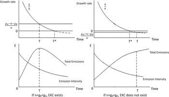
The GSM utilizes a simple neoclassical growth framework to analyze how pollution evolves alongside the process of economic development. The most important conclusion of the GSM is that the inverted-U shaped EKC exists only when n + g B < g A ; otherwise, pollution emissions will continuously increase over time without any turning point.Footnote 6 This conclusion is intuitively depicted in the left panel of figure 2.
The GSM and its relationship to the EKC

As shown in the upper half of the left panel of figure 2, when n + g
B
< g
A
, the horizontal line corresponding to
 $\dot{E}/E=0$
crosses the vertical axis at
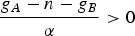 $\displaystyle{{g_{A} -n-g_{B}} \over {\alpha}} \gt 0$
; therefore, the total emissions peak at time T, ahead of the time T* when the economy arrives at the steady state because T* is actually the time when
 $\dot{k}/k=0$
. In this case, the turning point of CO2 emissions would occur before the economy enters the steady state; therefore, the inverted-U shaped EKC would exist. In contrast, as shown in the right panel of figure 2, if n + g
B
> g
A
, then
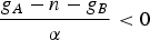 $\displaystyle{{g_{A} -n-g_{B}} \over {\alpha}} \lt 0$
, and CO2 emissions would not reach a maximum before the economy reaches the steady state at time T*. In this case, the total emissions would monotonously increase along the transition path before T* as the economy approaches the steady state; after time T* the emissions would still continue growing at a steady rate. As a result, if n + g > g
A
the inverted-U shaped EKC would not be observed.
3. Empirical tests for a GSM prediction: convergence in per capita CO2 emissions across provinces
An important prediction of the GSM is that there will be convergence in per capita emissions of the pollutants if n + g B < g A when the inverted-U shaped EKC exists. Because the purpose of this research is to utilize the GSM as a theoretical framework to investigate whether there will be a turning point in total CO2 emissions, the convergence of provincial CO2 emissions should first be tested. The reason for this test is three-fold. First, as Ordás Criado et al. (Reference Ordás Criado, Valente and Stengos2011) note, in the long run, growth is sustainable only when the pollutants' pollution levels are stabilized. As a result, if the convergence does not exist, the provincial per capita CO2 emissions would not finally reach a steady level because the provinces where per capita CO2 emissions grew faster would keep growing more rapidly in terms of per capita CO2 emissions. In other words, the existence of the convergence is a necessary condition for the occurrence of a turning point in CO2 emissions (Jobert et al. Reference Jobert, Karanfil and Tykhonenko2010). Secondly, the existence of convergence in the per capita CO2 emissions across Chinese provinces indicates that the actual data for China are applicable to the GSM framework. Therefore, the GSM can indeed be utilized to forecast China's CO2 emissions. Thirdly, the values of certain important parameters such as output elasticity of capital stock (α) can be calculated based on the estimation results for the convergence, which makes forecasts based on the GSM more objective and reasonable.
3.1. Methodology
Parallel to the convergence in economic growth rate derived from the textbook Solow model, a direct prediction of the GSM is a convergence in per capita CO2 emissions across provinces. This prediction asserts that an economy with lower initial per capita CO2 emissions tends to experience faster growth in per capita CO2 emissions than economies with higher initial per capita CO2 emissions. Concretely, this ‘catch-up’ process can be described by the following equation, which is directly derived from the set-ups of the GSM:Footnote 7
 $$\eqalign{\displaystyle{{1} \over {N}}\ln \lpar e_{it}^c /e_{it-N}^c\rpar & = \beta_0 +\beta_1 \ln \lpar e_{it-N}^c\rpar +\beta_2 \ln \lpar s_i\rpar +\beta_3 \ln\lpar 1-\theta_i\rpar \cr & \quad +\beta_4 \ln [ \lpar n+g_B +\delta\rpar _i] +\varepsilon_{it} \cr \beta_0 & = g_B -g_A +1/N\lpar 1-e^{-\lambda N}\rpar \log\lpar \overline{\Omega_{t-N} B_{t-N}}\rpar \cr \beta_1 & =-1/N\lpar 1-e^{-\lambda N}\rpar \cr \beta_2 & =[ \alpha /\lpar 1-\alpha\rpar ] \cdot 1/N\lpar 1-e^{-\lambda N}\rpar \cr \beta_3 & =[ \alpha /\lpar 1-\alpha\rpar +\epsilon-1] \cdot 1/N\lpar 1-e^{-\lambda N}\rpar \cr \beta_4 & =-\beta_2 \cr \varepsilon_{it} & =1/N\cdot \lpar 1-e^{-\lambda N}\rpar \log\lpar \Omega_{i\comma t-N} B_{i\comma t-N} /\overline{\Omega_{t-N} B_{t-N}}\rpar +\sigma_{it}\comma \; }$$
where i represents the ith economy, N is the number of years in the sample, λ = [1 − α][n + g
B
+ δ] is the convergence rate toward the steady state, and Ω
i,t−N
B
i,t−N
is the product of abatement technology level and productive technology level, representing the synthesized technology level of the ith economy.
 $\overline{\Omega_{t-N} B_{t-N}}$
is the average value of the synthesized technology levels for all economies at time t − N. ε is a parameter of a concrete abatement function a(θ). σ
it
is an i.i.d error term. All the other variables and parameters have been defined in section 2.
Equation (4) can be used to test the convergence. If the key coefficient, β1, is estimated to be negative as predicted by theory, then the convergence in per capita CO2 emissions across provinces during the sample period is verified. Because other explanatory variables such as ln(s) and ln(n + g B + δ) are introduced in (4), the conditional convergence is tested.
Equation (4) is usually estimated by ordinary least squares (OLS) with cross-section data. However, the commonly known problem of heterogeneity would cause the OLS estimates to be biased.Footnote 8 In addition, the limited freedom of the cross-section data may also affect the reliability of the estimation result. In order to effectively tackle the heterogeneity problem and make full use of the potential of our data sample, as suggested by Weeks and Yao (Reference Weeks and Yao2003) and Ding and Knight (Reference Ding and Knight2009), (4) is reorganized into equation (5) with a lagged dependent variable on the right-hand side:
 $$\eqalign{\ln \lpar e_{it}^c\rpar & = \gamma_0 +\gamma_1 \ln \lpar e_{it-N}^c\rpar +\gamma_2 \ln \lpar s_i\rpar + \gamma_3 \ln \lpar 1-\theta_i\rpar \cr & \quad +\gamma_4 \ln [ \lpar n+g_B +\delta\rpar _i] +\mu_{it} \cr & \gamma_0 = N\beta_0\; \quad \gamma_1 = 1+N\beta_1\; \quad \gamma_2 =N\beta_2\; \cr & \gamma_3 = N\beta_3\; \quad \gamma_4 =N\beta_4\; \quad \mu_{it} =N\varepsilon_{it}.}$$
Then, we set N = 1 and utilize the dynamic panel data to estimate equation (5). In (5), a positive coefficient of ln(e c it−N ) less than 1 is indicative of the existence of conditional convergence. Because (5) incorporates dynamics and could control for endogeneity using GMM, we use (5) as the benchmark equation in the empirical study. There are generally two estimation methods for dynamic panel data, namely the first-differenced GMM and the system GMM. Because the latter has a superior finite sample property and is consistent even when there are measurement errors and endogenous right-hand side variables, in the context of empirical growth research, we employ the panel data system GMM estimator as our prior estimator.Footnote 9
3.2. Data
3.2.1. Chinese provincial CO2 emissions
Because there are no official statistics available to date for CO2 emissions in China, we have to estimate the provincial emissions ourselves. The estimation is conducted according to equation (6) below. The first item in the square brackets represents the CO2 emissions from fossil fuel combustion, which are estimated according to IPCC (2006). The second item, CE, represents the CO2 emissions generated from cement production.Footnote 10
 $$EC_i = \sum_{j=1}^m [ \lpar F_{ij}\cdot CF_{ij} \cdot CC_{ij} -SC_{ij}\rpar \cdot OF_{ij}] +CE_i $$
The meanings of the parameters in (6) are as follows: the subscript i represents province i and the subscript j, the energy of type j; m is the number of energy types. EC denotes the CO2 emissions, F is the fuel consumption, CF is the fuel's calorific factor, CC is the fuel's potential carbon emission factor, SC is the fuel's carbon sequestration, and OF is the fuel's fraction of carbon oxidized. For each fuel type, the values of CF, CC and OF suggested by IPCC (2006) are used directly.
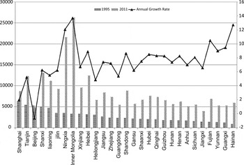
The consumptions of various types of fuels are taken from the China Energy Statistics Yearbook (1996–2012). Because the provincial carbon sequestration productions are unavailable, we simply ignore the item SC ij .Footnote 11 The provincial cement production data are obtained from the China Economic Information Network. Because provincial consumption data are not available prior to 1995, the time span of our sample period is from 1995 to 2011.Footnote 12 Figure 3 shows the ranking of provinces sorted by per capita CO2 emissions in the first available year, 1995. It can be observed from figure 3 that, during our sample period 1995–2011, provinces with lower per capita CO2 emissions (such as Yunan, Guangxi and Hainan) experienced faster growth in per capita CO2 emissions than provinces with higher per capita CO2 emissions (such as Shanghai, Tianjin and Beijing), suggesting that a convergence in per capita CO2 across provinces most likely exists.
1995 and 2011 provincial per capita CO2 emissions (kilos) and average annual growth rate over sample period (%)

3.2.2. Other data
The textbook Solow model is for a closed economy, in which the savings rate is equal to the investment rate. However, considering China's huge scale of foreign business, this assumption does not hold. Instead, following Weeks and Yao (Reference Weeks and Yao2003) and Ding and Knight (Reference Ding and Knight2009), the fixed-asset investment rate is used as the value of s in equations (4) and (5).
There has previously been considerable controversy over the estimation of the capital depreciation rate, δ. Some scholars prefer to take a constant value of δ for all provinces (e.g., Zhang and Zhang Reference Zhang and Zhang2003; Guo and Jia Reference Guo and Jia2004). However, because the difference in δ is an important cause of the difference in growth rates and CO2 emissions across provinces, we calculate provincial capital depreciation rates using real capital stock data estimated by He et al. (Reference He, Zhang and Shek2007).
For the population growth rate n, we use the growth rate of the provincial residential population rather than the registered population because the residential population makes a direct contribution to local economic development and CO2 emissions whereas, under the current household registration system, the migrant workers working and living in a province are usually still registered at their birthplaces elsewhere.
The value of productive technology progress, g B , is also highly controversial. Although some studies report no statistically significant technology progress in China (such as Kong et al. Reference Kong, Marks and Wan1999 and Wu Reference Wu2000), most studies estimate technology progress to be positive in China during the post-reform period (such as Young Reference Young2003 and Cao Reference Cao2007). The estimated technology progress in productivity since the mid-1990s has been relatively stable and fluctuates within a small range between 1 and 2 per cent.Footnote 13 For the nationwide technology progress, we set g B = 1.5 per cent. Because the eastern region has the highest rate of technology progress, whereas the western region is estimated to have the lowest rate (Wang et al. Reference Wang, Gong and Cheng2006), we set the technology progress rates for eastern, central and western China at 1.8, 1.5 and 1.2 per cent, respectively.Footnote 14
The parameter θ represents CO2 abatement cost as a ratio of GDP. Due to the unavailability of data on the specific investment for CO2 emission abatement, we simply take the average ratio of total investment in environmental protection to GDP during the sample period as the value of θ.Footnote 15 Because θ is accessible only after 2002, and because the value of θ is relatively stable for each province (the variation range for θ is usually less than 1 per cent), we combine ln(1 − θ) in equations (4) and (5) into the constant term.Footnote 16
3.3. Estimation results
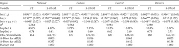
In order to test the convergence nationwide and within regions, we estimate dynamic equation (5) with the data from all provinces and the provinces in the three regions, respectively. The results are presented in table 1. In order to test the potential influences of endogeneity, the estimates of traditional fixed effects (FE) and system GMM (S-GMM) are both reported.
Estimation results of equation (5) for the whole country and the three regions

Notes: Robust standard errors are given in parentheses. All test results are given as p-values. FE and S-GMM stand for fixed effects and system GMM methods, respectively. Following Ding and Knight (Reference Ding and Knight2009), in the system GMM estimations, ln(e c t−1) is treated as a predetermined variable; ln(s) and ln(n + g B + δ) are treated as endogenous variables. Implied convergence rate λ and the output elasticity of capital stock α are calculated according to the definitions of coefficients γ 1 and γ 2 in equation (5). Significance at the 1%, 5% and 10% levels is indicated by *, ** and ***, respectively.
In table 1, we can clearly observe that the coefficients of ln(e c t ) are indeed significantly positive and lower than 1 for China and its three regions, implying that a conditional β -convergence in per capita CO2 emissions exists across the provinces within the whole country as well as within each region.
An interesting finding is that the implied convergence rates of per capita CO2 in the central and western regions of China are greater than that in the eastern region, suggesting that the intra-area differences in per capita CO2 emissions in the central and western provinces are considerably larger than within the eastern provinces. The existence of convergence also implies that the provincial per capita CO2 emissions tend to stabilize in the long run, which creates the possibility for the occurrence of a turning point in total CO2 emissions for the three regions as well as for the whole country. The existence of convergence in per capita CO2 emissions also provides some hints to policy makers on how to set up differential policies to control for the regional growth of CO2 emissions in a more reasonable and efficient way: provinces with relatively high CO2 emissions per capita should be assigned tougher targets for emissions reductions and faster reduction rates, whereas provinces with relatively low carbon intensity should be allowed to cut emissions at a lower rate.
4. Forecasting China's CO2 emissions
4.1. Parameters settings
Given the regional gaps in economic development and the remarkable differences in the patterns of energy consumption and CO2 emissions between the three regions of China, it is more reasonable to project China's CO2 emissions based on forecasts for each region. As stressed by You (Reference You2013), forecasting using disaggregated information (e.g., Auffhammer and Carson Reference Auffhammer and Carson2008) can improve the accuracy of the forecasts because regional heterogeneity can be taken into account. We project CO2 emissions for the eastern, central and western regions, individually, and then forecast for the whole country by adding the projected regional emissions together. In order to make reasonable and reliable forecasts, the settings of the related parameters in the GSM (α, s, δ, θ, n, g A and g B ) are critical. In this subsection, we discuss the proper values for these parameters for each region of China.
The output elasticity of capital stock, α, can be estimated based on the regression results for the convergence analysis (see table 1). We take the values of implied α for the three regions on the basis of system GMM estimates because the GMM method accounts for the potential endogeneity problem and therefore produces more reliable estimates. Specifically, the values of α for eastern, central and western regions are chosen as 0.69, 0.69 and 0.71, respectively. This choice is consistent with previous studies estimating that α ranges between 0.55 and 0.85 for China's economy (Chow and Lin Reference Chow and Lin2002; Cao Reference Cao2007; Li and Zeng Reference Li and Zeng2009).Footnote 17 The value for saving rate (s), depreciation ratio (δ) and the share of CO2 abatement cost to GDP (θ) are the same as discussed previously for the estimation of convergence.
As defined, g B is the productivity growth rate. According to our calculations from the empirical estimation section, the values of g B for the eastern, central and western regions are 1.8, 1.5 and 1.2 per cent, respectively.
The exogenous growth rate in carbon efficiency, g A , is a key parameter for determining whether the inverted-U shaped EKC exists. A natural idea is to set g A as the rate at which the CO2 emission intensity of GDP decreases over time. However, this treatment has two main flaws. First, the decrease in CO2 emission intensity cannot fully reflect an advance in carbon efficiency. For instance, even if the carbon efficiency remains unchanged, when the non-energy factor inputs of the economy (such as labor and capital) grow faster than the energy input, the CO2 emission intensity would decrease, and vice versa. Secondly, the level of CO2 emission intensity of GDP is to some extent influenced by economic cycles. For example, during China's economic boom period between 1995 and 1998, CO2 emission intensity decreased relatively rapidly, whereas during the economic downturn from 2008 to 2011, the overall CO2 emission intensity hardly declined, and even rose slightly in some provinces. Despite these flaws, in the medium and long run, the evolvement of CO2 intensity would still reflect the effects of technology progress in carbon efficiency. As a result, in this study we take the annual rate of decrease in CO2 intensity during 1995 and 2007 as a reference rather than an exact value for g A . The corresponding rates for the eastern, central and western regions for the period 1995–2007 are 4.0, 4.3 and 3.0 per cent, respectively.Footnote 18 Another reference for g A is the changes in government staff devoted to environmental protection, as suggested by He and Wang (Reference He and Wang2012).Footnote 19 Utilizing data from the China Statistical Yearbooks on Environment (1996–2012), the average annual growth rates of the government staff specialized in environmental protections are calculated to be 4.2, 5.3 and 5.6 per cent for the eastern, central and western regions, respectively. We simply take the average of these two references for g A as the benchmark values of g A in corresponding regions. Therefore, for the eastern, central and western regions, the values of g A are set to 4.1, 4.8 and 4.3 per cent, respectively. It is noteworthy that the difference between the two references of g A for the western region is considerably larger than that for the eastern and central areas. Considering the fact that g A is crucial for the potential existence of a turning point in CO2 emissions, different possible values of g A are tested in the sensitivity analysis in the next section.
During the sample period between 1995 and 2011, the growth rates for the residential population in the eastern, central and western regions were 1.2, 0.26 and 0.33 per cent, respectively. Although China has recently eased its one child policy that has been in place for over two decades, the relatively low population growth is expected to persist.Footnote 20 Considering the fact that the regional differences between the eastern and inland provinces will most likely be reduced over time, there are predicted to be fewer workers migrating from inland provinces to coastal areas for higher paying jobs. As a result, the population growth rate of the eastern region may be slightly lower than its average annual growth rate in the last two decades, whereas the population growth rates of the central and western regions may be slightly higher than their respective historical average levels. Therefore, we set the population growth rates (n) in eastern, central and western regions at 0.8, 0.3 and 0.4 per cent, respectively.Footnote 21
Finally, the initial future economic growth rates projected for the three regions are set at the average growth rates during our sample period between 1995 and 2011. Based on the initial growth rate of GDP per capita, the dynamics of initial capital stock per effective worker in each region could be calculated according to the production function and the dynamic equation (1) for capital stock.
To summarize, the values of the parameters for China's three regions in the benchmark scenario are shown in table 2. It should be noted that, for each region, the condition for the existence of a turning point in CO2 emissions, n + g B < g A , is satisfied. Therefore, CO2 emission peaks will occur in all regions of China, suggesting that an overall turning point in China's CO2 emissions will appear at some time in the future.Footnote 22
Model parameterizations of the benchmark scenario

Note: γ0 represents the per capita GDP growth rate at the initial time of the projection (2011).
4.2. Forecast results
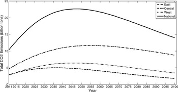
Once the key parameters of the GSM and the initial GDP growth rates are fixed, the dynamics of China's CO2 emissions as well as economic growth are completely determined according to equations (1)–(3). Before the forecast is conducted, the credibility of the GSM framework is first examined. The sample period is split into two subperiods (1995–2006 and 2007–2011), and the in-sample forecasts of CO2 emissions for the three regions and the whole country are made for the last five years of the sample period (2007–2011). The in-sample forecast results are close to the actual emissions, and the relative errors of forecast (the ratio of forecast error to the actual data) are within 5 per cent in most years for the three regions and the whole country.Footnote 23 The in-sample forecast results verify the credibility of the fit of the model to the actual data; therefore, it can be used to make an out-of-sample forecast. Figure 4 plots the projected total CO2 emissions for the three regions and for China as a whole from 2011 to 2100 (black lines in figure 4).
China's projected national and regional total CO2 emissions from 2011 to 2100 in the benchmark scenario

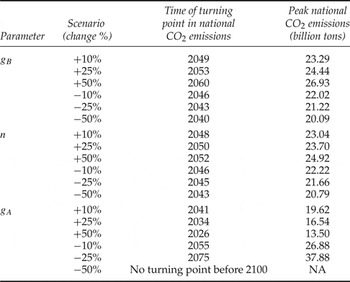
As shown in figure 4, in the benchmark scenario, the turning point in total CO2 emissions will occur in the year 2047, and the emission peak will reach 22.62 billion tons at that time. Because the forecast results are highly dependent on the values of key parameters in the GSM, it is necessary to perform a sensitivity analysis based on the choices of some important parameters over the range of possible values. Because the condition for existence of a turning point is that g B + n < g A , we focus on these three key parameters. In order to take the uncertainty into full consideration, we allow for variation as much as 50 per cent from the benchmark scenario level. Specifically, we make repeated calibrations with one of the three key parameters changing ±10 per cent, ±25 per cent and ±50 per cent, while keeping the other two parameters unchanged. For each scenario, we examine whether and when the turning point in total CO2 emissions occurs and the corresponding total CO2 emissions at that point. The results for the sensitivity analysis are reported in table 3.
Calibration results for the different scenarios in the sensitivity analysis

Note: In each alternative scenario, a specific parameter is altered while all the other parameters are kept constant.
As shown clearly in table 3, the time at which the turning point occurs is most sensitive to the growth rate in carbon efficiency (g A ). A decrease in g A by 10 per cent would delay the occurrence of the emission peak by nearly a decade. If the g A is 50 per cent lower than the benchmark level, the turning point would not occur before 2100.Footnote 24 Comparatively, changes in the other two parameters do not alter the timing and level of the emission peak significantly.Footnote 25 ,Footnote 26
5. Conclusions
As China's economy boomed, China's total CO2 emissions proliferated at a dramatic rate. Since 2007, China has become the largest CO2 emitter in the world; in 2010 China contributed nearly a quarter of global total CO2 emissions. The surge in China's CO2 emissions has caused increasing international concern, and the domestic pressures from an increasing gap in energy demand and the deteriorating environment are also forcing the Chinese government to shift economic growth patterns to be more intensive and curb CO2 emissions. Despite the Chinese government's reiteration of this goal and implementation of policies to control CO2 emissions, skeptics doubting whether China can effectively hold CO2 emissions in check still exist at home and abroad.
In order to address the concerns about whether and when the turning point in China's CO2 emissions will occur, the emissions should be forecast in a reasonable and reliable way. A commonly used forecasting method is the EKC. However, due to some major problems in both theoretical and empirical aspects, the EKC is not directly employed for forecasting in this research. Instead, the prediction herein is based on a computable theoretical framework – the GSM. The GSM includes the basic characteristics of the textbook Solow model and incorporates CO2 emissions as an undesirable by-product. If the forces contributing to increasing CO2 emissions (including the scale effects caused by economic growth and population increases) grow less rapidly than the forces contributing to emissions reductions (abatement technology progress and investment in emission reduction), the emissions would stabilize at some time and then eventually decrease.
In order to examine whether the GSM framework is applicable to China's economy, a direct prediction of the GSM – that per capita CO2 emissions converge across provinces – is tested. Utilizing fixed effects and system GMM methods, the convergence in CO2 per capita across provinces across the whole nation as well as within three distinct regions of China is verified. The existence of convergence also implies that provincial per capita CO2 emissions tend to stabilize in the long run, which is a prerequisite for the existence of a turning point in CO2 emissions.
Considering the remarkable differences in development levels and energy consumption patterns across China's different regions, the national CO2 emissions are forecast using disaggregated regional information. After assigning reasonable values to the key parameters of the GSM for the three regions, the respective CO2 emissions between 2011 and 2100 for the eastern, central and western regions of China are projected. The predicted national CO2 emissions are the sum of the three regions' projected emissions. In the benchmark scenario, the turning point in China's total CO2 emissions would occur in about 2047, and the corresponding total emissions and per capita emissions would be approximately 22,622 million tons and 13,891 kg, respectively.
According to the sensitivity analysis, carbon efficiency is the most important factor in determining the existence of a CO2 emission peak. Other conditions being equal, a decrease in the progress rate of carbon efficiency (g A ) by 37 per cent would cause the collapse of the turning point, whereas a 10 per cent increase in g A would cause the turning point to occur six years earlier than in the benchmark scenario. As a result, enhancing the efficiency of energy usage and CO2 emissions and accelerating the technology progress of CO2 abatement techniques are vitally important for ensuring that the turning point in China's CO2 emissions occurs as early as possible.
Despite the merits of our forecast results based on the GSM, there is still ample room for further improvement of the GSM framework in both its theoretical and empirical aspects. For instance, the assumptions of exogenous productive technology progress and carbon efficiency could be relaxed. In addition, energy could be introduced in the production function as a separate input, so that the effect of the change in energy structure on CO2 emissions could be examined in more detail. These improvements represent possible future research directions that could provide a more sophisticated GSM framework and more reasonable and reliable forecast results.