1 Introduction
Legged robots can move on both regular and even irregular surfaces (Gerndt et al., Reference Gerndt, Seifert, Baltes, Sadeghnejad and Behnke2015; Shangari et al., Reference Shangari, Shamshirdar, Heydari, Sadeghnejad, Baltes and Bahrami2015; Navabi et al., Reference Navabi, Sadeghnejad, Ramezani and Baltes2017). A small area of their feet touches the ground, which means that legged robots can operate effectively. Although wheeled robots are easier and more convenient to be used on smooth surfaces and long distances because of their high speed, better stability and thus better control, the legged ones are more complex and extremely unstable in most cases, making them more difficult to be controlled (Shafei et al., Reference Shafei, Sadeghnejad, Bahrami and Baltes2014; Janati et al., Reference Janati, Abdollahi, Ghidary, Jannatifar, Baltes and Sadeghnejad2017; Yazdankhoo et al., Reference Yazdankhoo, Shahsavari, Sadeghnejad and Baltes2018). In many aspects, legged robots have more advantages than wheeled robots which make them impossible to be replaced in specific missions such as climbing the stair and walking on an uneven surface, etc. Biped robots are a kind of legged robots that are being structured such that they can mimic human-like movements (Moro et al., Reference Moro, Tsagarakis and Caldwell2011; Abbas Shangari et al., Reference Abbas Shangari, Sadeghnejad, Baltes, Goswami and Vadakkepat2016; Javadi et al., Reference Javadi, Azar, Azami, Ghidary, Sadeghnejad and Baltes2017) and perform specific tasks like activities in hazardous environments and help the elderly (Baltes et al., Reference Baltes, Hosseinmemar, Jung, Sadeghnejad and Anderson2015; Ott et al., Reference Ott, Roa, Schmidt, Friedl, Englsberger, Burger, Werner, Dietrich, Leidner and Henze2017; Shangari et al., Reference Shangari, Shams, Azari, Shamshirdar, Baltes and Sadeghnejad2017). Having a better perception of humans’ natural movements from biological and biodynamic points of view, producing artificial organs for sick and disabled people, utilizing the humanoid robots to work in hazardous environments that have the potential for explosions and fires and to carry out intolerable tasks which can have more mobility in the uneven paths such as moving on stairs and crossing obstacles in comparison with wheeled robots are some different applications of biped robots.
As a result, due to their high mobility capabilities and structural resemblance to humans, biped robots have attracted the attention of many researchers (Baltes et al., Reference Baltes, Sadeghnejad, Seifert and Behnke2014; Baltes et al., Reference Baltes, Bagot, Sadeghnejad, Anderson and Hsu2016; Baltes et al., Reference Baltes, Tu, Sadeghnejad and Anderson2017b). Our main contribution is to have a small effect in the rehabilitation field to prepare correct walking pattern for humans who have a problem with their walking, so we optimize the problem in such a way that minimizes the power consumption with maximizing the system stability and also consider the effect of average speed and walk in a way that most similar to a human walking. Hence, stability and power consumption of the robot, respectively, reached their highest and lowest value (the most optimal mode), and the robot walked like a human as far as possible. So, walking abilities of the robot were in the best case of energy, stability and motion speed and were human-like as far as possible.
In the next section, previous studies conducted on biped robots and related literature were presented and finally, the problem was defined.
2 Related works
In recent years of humanoid robot studies, different researches tried to develop different humanoid platforms. In 1973, Kato constructed the first biped robot known as Waseda at the University of Waseda, Japan (Lim & Takanishi, Reference Lim and Takanishi2007). In 1990, McGeer described the concept of passive biped robots and from 1993 to 1997, Honda Corporation built the first humanoid robots in three models P1, P2 and P3 (Liu et al., Reference Liu, Tan and Zhao2007). Among the most prominent humanoid robots known today, ASIMO made by Honda, HRP made by Kawada Company and QRIO of Sony can be mentioned (Akachi et al., Reference Akachi, Kaneko, Kanehira, Ota, Miyamori, Hirata, Kajita and Kanehiro2005; Kaneko et al., Reference Kaneko, Harada, Kanehiro, Kimura, Miyamori and Akachi2008).
The various aspects of studies on biped robots are dynamic and kinematic modeling, walking, stability, path prediction and optimization of power consumption. In order to explain robot walking, the kinematic and dynamic behavior of a robot during walking and corresponding mathematical equations must be extracted. Direct or forward kinematics can be written when the coordinates of robot joints are specified and position and orientation of the links of the robots are also identified as the functions of those aforementioned coordinates. Also, in inverse kinematics, these procedures can be done conversely. Hence, inverse kinematics could be very useful in determining the control of individual joints which is necessarily required in the entire walking cycle of the biped robots. The outputs of inverse kinematics calculations provide us with the desired reference movement for control purposes. In order to obtain differential equations of the system, two common methods are used: Lagrange equation and Newton–Euler one. In a direct dynamic method, the system motion differential equation is solved through an active force/torque vector as an input. Further, the right control rule is chosen to create the input controls (torques/forces) that follow the desired reference path in a robot mechanism. In 1985 and 1986, Todd (Reference Todd2013) carried out extensive research on the dynamic balance of biped robots. In 1992, Shih and Gruver (Reference Shih and Gruver1992) studied the dynamics and control of the biped robots during the double support phase. They used springs and dampers in two vertical and horizontal directions in their contact model. In 2004, Mu and Wu (Reference Mu and Wu2006) investigated the impact effect created at the end of the single support phase on robot dynamics. Path prediction plays a crucial role in the stability of biped robots. The purpose of gait planning is to determine the trajectory of joint variables in such a way that the robot follows the desired movement.
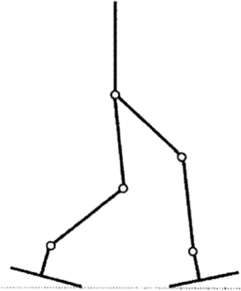
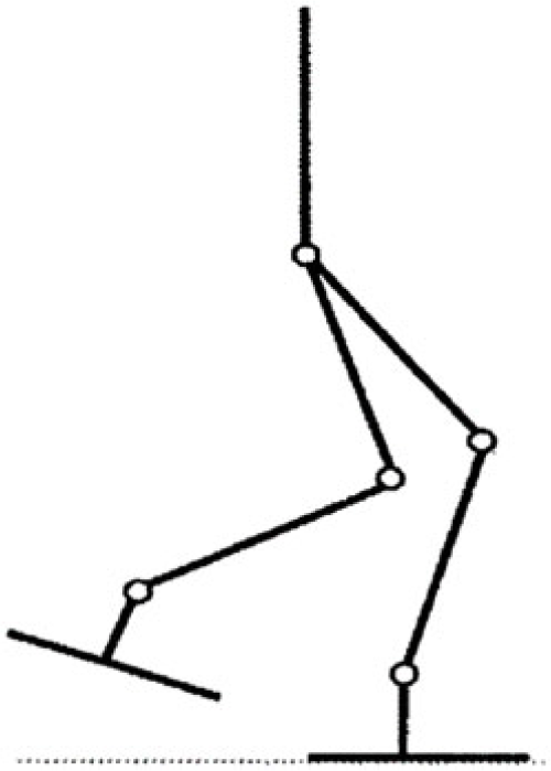
The performance of biped locomotion has been improved in recent years, using various methods, but this is still too far from being stable and energy efficient comparing with a human walk (Larsen & Stoy, Reference Larsen and Stoy2011; Baltes et al., Reference Baltes, Tu, Sadeghnejad and Anderson2017a; Shams Esfand Abadi et al., Reference Shams Esfand Abadi, Rahmati and Sadeghnejad2018). Therefore, the analysis of human gait is one of the most challenging and important tasks in order to develop energy-efficient algorithms of human-like robot locomotion (Asano & Luo, Reference Asano and Luo2008). For human-like walking of a biped robot, first human walking was considered. Human walking is a cyclical motion that can be separated into two phases: double support and single support. The double support phase occurs when both feet are on the ground and the entire body moves (Figure 1). This phase will create a closed kinematic chain. The single support phase happens when only one foot is planted on the ground and the other foot moves forward (Figure 2).
Robot model in the double support phase (closed kinematic chain)

Robot model in the single support phase (open kinematic chain)

This phase will create an open kinetic chain. Joints, muscles and other anatomical structures function differently in open-chain (non-weight-bearing) and closed-chain (weight-bearing) positions during the gait cycle. The impact phenomenon will also occur at the end of this phase.
One of the most important issues, discussed in the biped robots design, is how to keep their balance while walking. The balance of the biped robots can be divided into two parts: static balance and dynamic balance. Accordingly, various criteria have been developed to ensure the stability of biped robots. The center of mass is a criterion to measure the robot’s static balance. As a matter of fact, static balance can only guarantee the robot’s balance in the absence of strong dynamic influences; therefore, the motion speed must be very low. One of the most important measures of dynamic balance is Zero Moment Point (ZMP). This concept was first introduced by Vukobratović and Stepanenko (Reference Vukobratović and Stepanenko1972). In 2004, Vukobratović and Borovak (Reference Vukobratović and Borovac2004) completed and clarified the concept. Then, Sardain and Bessonnet (Reference Sardain and Bessonnet2004) designed and developed a mechanical shoe, equipped with power sensors to express the connection between ZMP and the pressure center (Sardain & Bessonnet, Reference Sardain and Bessonnet2004).
Many approaches have been developed to ensure the stability of robots during stepping. In many of these studies, the ideal path of the ZMP is predefined in advance which is used then to achieve joints trajectory. In these methods, it is not possible to create a smooth path which minimizes the expend energy because the ideal path that predefined may not be the best case and so increase the power consumption of robot during walking. To solve this problem, some other researchers designed hip and ankle joints paths first. Then, the two unknown parameters in the hip joint design are calculated in a way that provides the highest stability margin for the robot studied.
In this paper, we use the Newton–Euler method during the single support phase to investigate the robot’s dynamics. ZMP will be considered as a criterion of robot stability. It is of great importance to use inverse kinematics in order to employ the stability criterion. Initially, we try to turn joint positions into joint angles using the Jacobin matrix. Then, the joint angles, angular velocities and angular acceleration will be calculated and added then we calculate the position of the ZMP. Dynamics of the problem will also be used to calculate the kinetic and potential energy. Finally, the joint torques will be calculated. In addition to the maximum stability, we will attempt to improve the robot motion by calculating the energy using joint torques. Further, ZMP and energy values will be combined to calculate the maximum stability and minimum consumed energy. Since the optimization problem is nonlinear, a parametric optimization method will be used to solve it. On the other hand, the joint angles were defined as the parametric functions so the coefficients were determined through the parametric optimization in such a way that the objective function obtained was minimized. In the end, the effect of motion average speed on total energy consumption was considered and the optimum average speed of biped locomotion was obtained.
This paper is structured as follows. Section 3 presents the model and motion equation extraction of biped robot. Section 4 discusses the power consumption optimization and introduces cost function and constraints. Section 5 investigates the effect of motion average speed on energy consumption and obtains optimum average speed for the motion of the biped robot. Finally, Section 6 comments on the experimental test that performed for validation basis; in Section 7, implementation and results were expressed and at the end, conclusion of the work is expressed in Section 8.
The biped robot model

3 System dynamics
3.1 The biped robot dynamic model
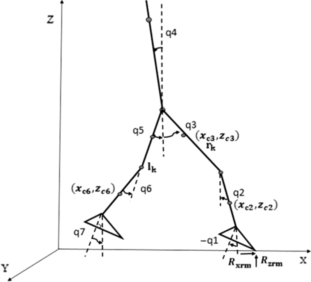
The seven-link dynamic model of a biped robot is considered for this study (Figure 3). These nine degrees of freedom mechanism introduced the fourth linkage as the trunk, the third and fifth as two components of the thigh, the sixth and second as shins and the first and seventh are taken as the robot’s feet. All linkages are connected to each other through six joints, that is, 3 and 4 as the hip joints, 5 and 2 as the knee joints and 1 and 6 as the two ankle joints. There is an actuator embedded in every joint, and it is assumed that all joints are friction-less and only have a rotational movement in the main longitudinal (sagittal) plane.
During normal walking, the robot will spend the vast majority of the time in the single support phase. Indeed, for quick walking, the minimization of the time in double support phase is crucial. We, therefore, focus on the dynamics of the system in the single support phase.
Thus, a constant value is defined for the horizontal and vertical position of the one toe, and two degrees of freedom are eliminated.
Therefore, a biped robot with nine degrees of freedom is turned into a robot with seven degrees of freedom. The geometric and inertial parameters are defined as follows: m i is the mass of each linkages (according to the mass of anthropometric dimensions explained by the Winter book) (Winter, Reference Winter2009), I i is the moment of inertia of each linkages that revolves around the axis passing through the center of mass and is perpendicular to the longitudinal plane, l i is the length of each linkage, d i is the distance between the center of mass and of each linkage and the next joint (upper) which is stated based on the part of linkage’s length, q i is the absolute angle of each member to the perpendicular line counter clockwise and  $x_{{c_i}}$
is the position of each linkage’s center of mass.
3.2 Extracting the equations of motion
The relationships between kinematic parameters and force parameters in a dynamical system are expressed by its equations of motion. The number of independent equations of motions for every dynamical system is equal to the number of degrees of freedom. In this section, the kinetic and dynamic equations observed in every linkage are extracted. Note that, there are various methods for deriving the dynamic equations.
Among the most important techniques developed in this regard, Newton–Euler, Lagrange and Kane’s methods can be specified (Gillespie & Colgate, Reference Gillespie and Colgate1997). In this research, dynamic equations of the biped robot were extracted according to Equation (1), using the Recursive Newton/Euler method in a single support phase which M(y), C(y) and G(y) are polynomial functions of joints.
 \begin{equation}{\rm{M}}(y)\ddot y + {\rm{C}}(y)\dot y + {\rm{G}}(y) - {\boldsymbol{\tau} ^{{\rm{GRF}}}} = {\boldsymbol{\tau} ^{\rm{M}}}\end{equation}
 ${\rm{C}} \in {\textbf{R}^{{{\rm{n}}_{\rm{y}}} \times {{\rm{n}}_{\rm{y}}}}}$
refers to the Coriolis matrix. Gravity vector is defined as
 $ \in {\textbf{R}^{{{\rm{n}}_{\rm{y}}}}}$
. Also
 ${\boldsymbol{\tau} ^{{\rm{GRF}}}},{\boldsymbol{\tau} ^{\rm{M}}}$
, respectively, refer to the torque vector of Ground Reaction Force (GRF) at the contact point with the ground and the motors on robot joints.
To this end, the kinematic and dynamic equations of the right foot are extracted first and then the backward recursive equations are obtained. The same steps are repeated for the left foot and then equations of both feet are linked to each other through the robot trunk.
4 Power consumption optimization of a biped robot
A lot of researchers and efforts have been taken to achieve the robot’s motion path based on maximum stability which is assessed through ZMP. One of the shortcomings of the proposed method is that the obtained path usually raises the energy consumption. Thus, the present study aims to achieve the motion path by minimizing the energy as well as maintaining the stability of the robot by using optimization methods. Since walking is a periodic movement, the Fourier series is used in this study to estimate the joint angles. The optimization process is as follows: first, the joint angles are estimated by the third-order Fourier series. Employing the optimization algorithms and taking into account the kinematic constraints, then, these coefficients are changed in such a way that the objective function is minimized and ZMP remains within the supporting polygon region with the smallest distance from its center during single support phase. In this study, the interior point optimization (IP) method was used to predict the motion path of biped robots.
4.1 The cost function
In order to predict the path within the allowed range of stability, accompanied by the reduction of energy consumption, the objective function is defined as a combination of energy and stability as follows:
 $$\begin{equation}{\rm{Taw}} = 1000 \times \left[ {\mathop \sum \nolimits {{\left( {\frac{{\left( {{{\rm{X}}_{{\rm{zmp}}}} - {{\rm{X}}_{{\rm{MS}}}}} \right)}}{{{{\rm{X}}_{{\rm{MS}}}}}}} \right)}^2}} \right] + \left[ \begin{array}{cc}
{\mathop \sum \nolimits {{\left( {\dfrac{{\left( {{\rm{taw}}{{\rm{y}}_1}} \right)}}{{12.3774}}} \right)}^2} + \mathop \sum \nolimits {{\left( {\dfrac{{\left( {{\rm{taw}}{{\rm{y}}_2}} \right)}}{{74.6046}}} \right)}^2} + \ldots }\\[10pt]{ \ldots . + \mathop \sum \nolimits {{\left( {\dfrac{{\left( {{\rm{taw}}{{\rm{y}}_6}} \right)}}{{45.09794}}} \right)}^2} + \mathop \sum \nolimits {{\left( {\dfrac{{\left( {{\rm{taw}}{{\rm{y}}_7}} \right)}}{{2.3361}}} \right)}^2}}\end{array} \right]\end{equation}$$
 \begin{equation}{x_{{\rm{ZMP}}}} = \frac{{\sum\nolimits_{i = 1}^n {\left\{ {{m_i}\big( {\mathop {{Z_i}}\limits^ - {\textbf{g}_z}} \big){x_i} - {m_i}\left( {\mathop {{x_i}}\limits^ - {\textbf{g}_x}} \right){Z_i} + {I_{yi}}{\alpha _{yi}}} \right\}} }}{{\sum\nolimits_{i = 1}^n {{m_i}} \left( {\mathop {{Z_i}}\limits^ - {\textbf{g}_z}} \right)}}\end{equation}
Where  ${x_{{\rm{ZMP}}}}$
refers to the position of ZMP which is obtained through Equation (3),
 ${x_{{\rm{Ms}}}}$
is the center of the supporting polygon that has maximum stability for the robot and
 ${\rm{taw}}{{\rm{y}}_{\rm{i}}}i = 1,2, \ldots ,7$
are joints torque. In Equation (3), m i refers to the mass of the robot inks,
 ${I_{{y_i}}}$
is the momentum of i linkage around the y-axis passing through the center of mass of each member and
 ${\alpha _{{y_i}}}$
is the absolute angular acceleration of each link.
 $\left( {{\textbf{g}_x},0,{\textbf{g}_z}} \right)$
refers to gravitational acceleration vector, and
 $\left( {{x_i},0,{z_i}} \right)$
defined as the coordinates of the center of mass of each link. In order to maintain the robot stability at any moment, the square of the difference between the position of ZMP and the center of supporting polygon, which has the highest stability, is minimized. In order to minimize energy consumption, the moments of joints were considered in accordance with Equation (2) in the criterion function and then each moment was divided by its maximum experimental value.
4.2 Constraints
The optimization problem, examined in this study, is a constrained optimization problem. After joint angles were defined as the parametric functions and with regard to the kinematic constraints that define the maximum and minimum limits of the angles, the problem was calculated in a way that robot’s stability is maximized and the energy consumed during motion is minimized. As displayed in Table 1, some constraints are considered in the single support phase to clarify the initial and final position of the joints. Since walking and stepping mean to move forward, a couple of constraints should be applied to the horizontal positions of the left toe (Xlmet), the right thigh (Xrhip), wrist and knees of both feet in order to provide such a forward movement. Some other constraints were determined to ensure the robot’s stability, that is, to place the ZMP position within the supporting polygon region at a minimum distance to its center which has the maximum stability. In order to correctly apply the vertical force of the foot touching the ground, some constraints on vertical GRF are considered. Besides, Coulomb’s Friction Law was used to achieve a proper and non-slippery step during the single support phase.
Dynamic and kinematic constraints applied to the adaptive biped robot model.

5 The effect of motion average speed on the total energy consumption
The purpose of this section is to examine the effect of average motion speed on optimal energy consumption. For this purpose, by having the range of average speed, total energy consumption is obtained. Finally, by using the total energy consumption diagram in terms of average speed, the effect of average speed on energy consumption of the robot was considered an optimum average speed that was obtained.
Because integral of joint torques should approximate energy, we consider the square of joints torque in each moment and then we calculate the sum of them that can define as a discrete form of integral. According to Equation (4.4), the average speed was achieved by the difference in the weighted average of the center of mass of links at the beginning and end of the single support phase divided to the time elapsed in this phase.
 \begin{equation}{x_{\rm{c}}} = \frac{{{m_1} \times {x_{{{\rm{c}}_1}}} + \ldots + {m_7} \times {x_{{{\rm{c}}_7}}}}}{{{m_1} + \ldots + {m_7}}}\end{equation}
 \begin{equation}\Delta x = {x_{\rm{c}}}\left( {{t_{{\rm{final}}}}} \right) - {x_{\rm{c}}}\left( {{t_{{\rm{initial}}}}} \right)\end{equation}
 \begin{equation}\Delta t = {t_{{\rm{final}}}} - {t_{{\rm{initial}}}}\end{equation}
 \begin{equation}{{\rm{V}}_{{\rm{ave}}}} = \frac{{\Delta x}}{{\Delta t}}\end{equation}
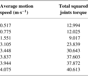
The result of the variation in average speed and its corresponding total energy consumption is shown in Table 2.
6 Experiments
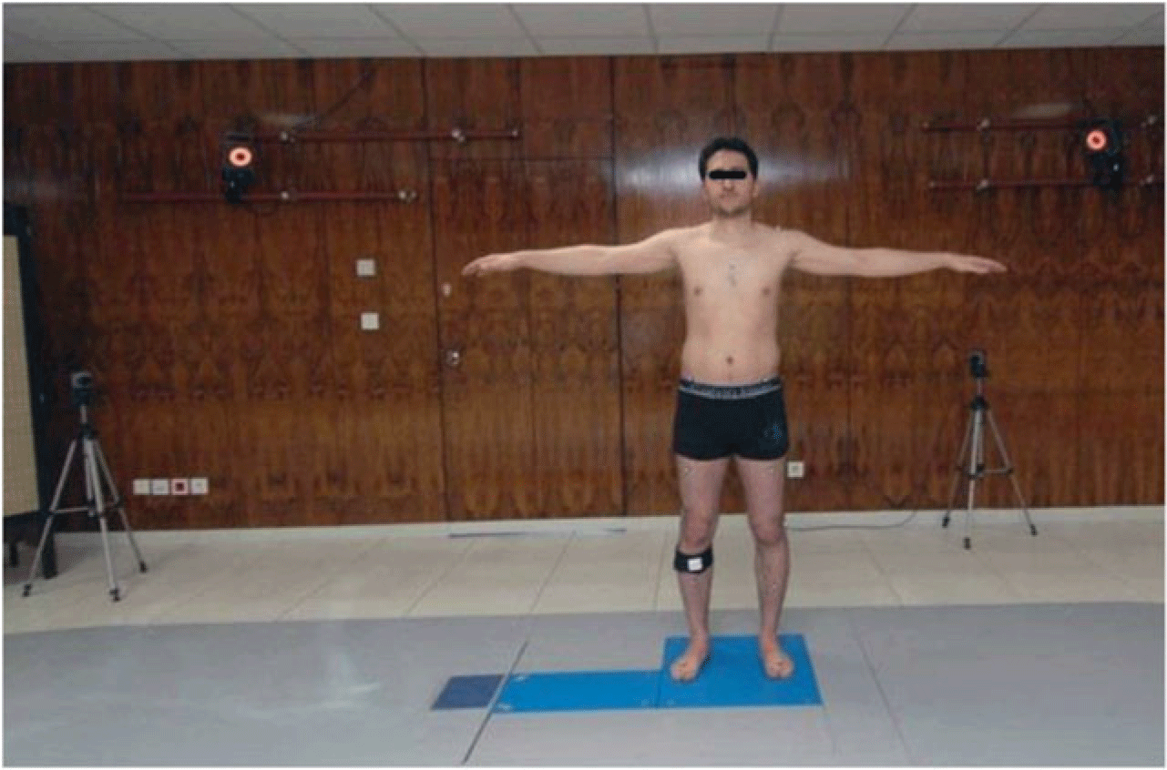
This section examines the experiments, required to analyze how a healthy person walks. In this study, a healthy male, age 29 years, was asked to do the gait analysis experiments. The experiments were performed at the Gait Analysis Laboratory of Dr Javad Movafaghian Research Centre of Intelligent Neural-Rehabilitation Technologies affiliated to the Sharif University of Technology (http://dmrcint.sharif.ir) (Figure 4). Experimental data, including kinematic motion and GRFs, were estimated by placing 28 markers, attached to anatomical positions and two power plates for a distance of more than one gait cycle at an average speed of 1.23 ± 0.1 m s−1. Five identical gait analysis experiments were performed on the target person; then, the average of kinematic information of the lower extremity was used as the optimal path for the biped robot model. Actions taken above can be generalized to all samples. After the extraction of the dynamic equations of the selected biped robot, Mathematica software was used to solve motion equations parametrically, and MATLAB was employed to solve them numerically.
The variation in the average speed and its corresponding total energy consumption.

The overview of a healthy participant examined in the Gait Analysis Laboratory

7 Results and validations
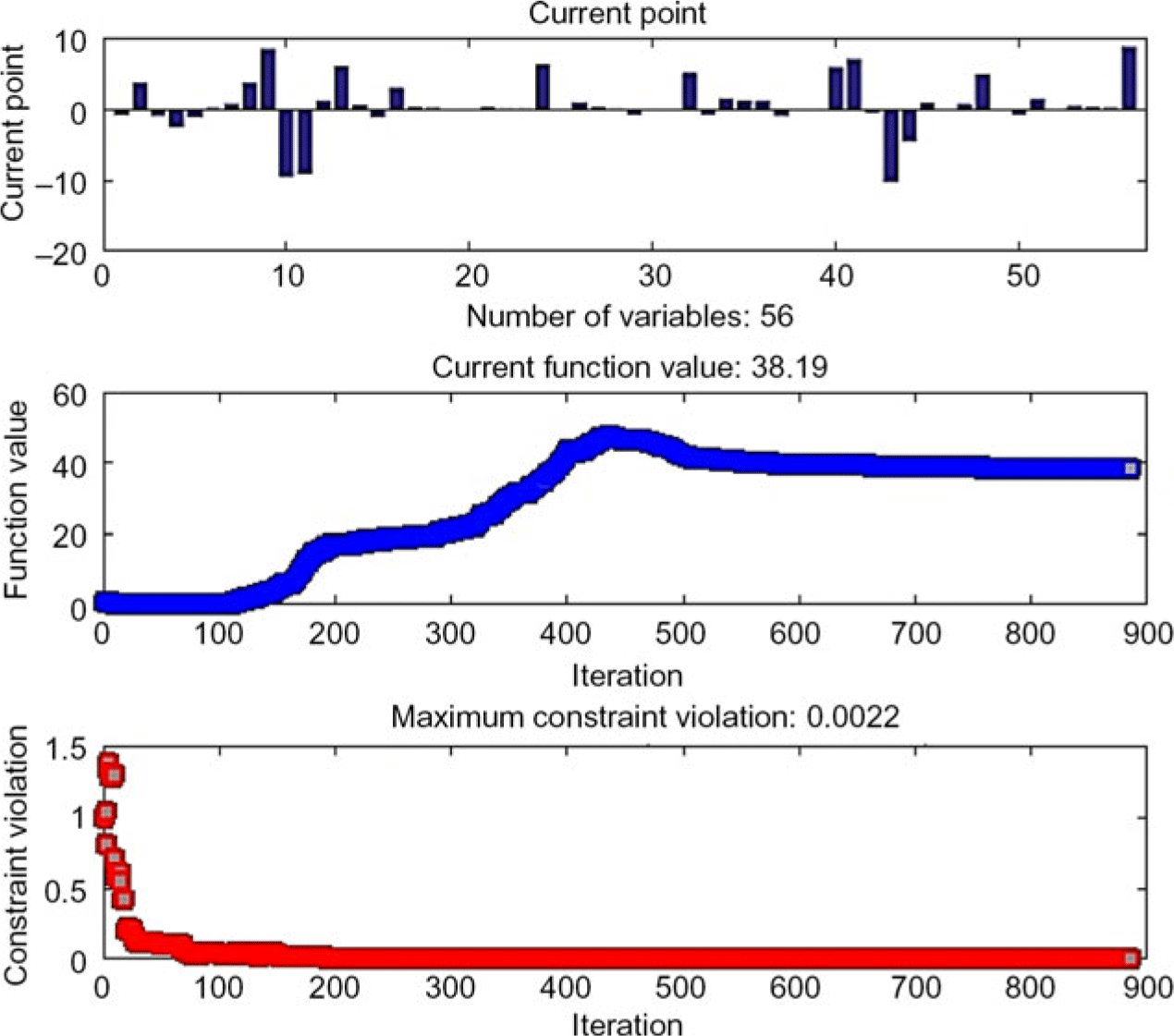
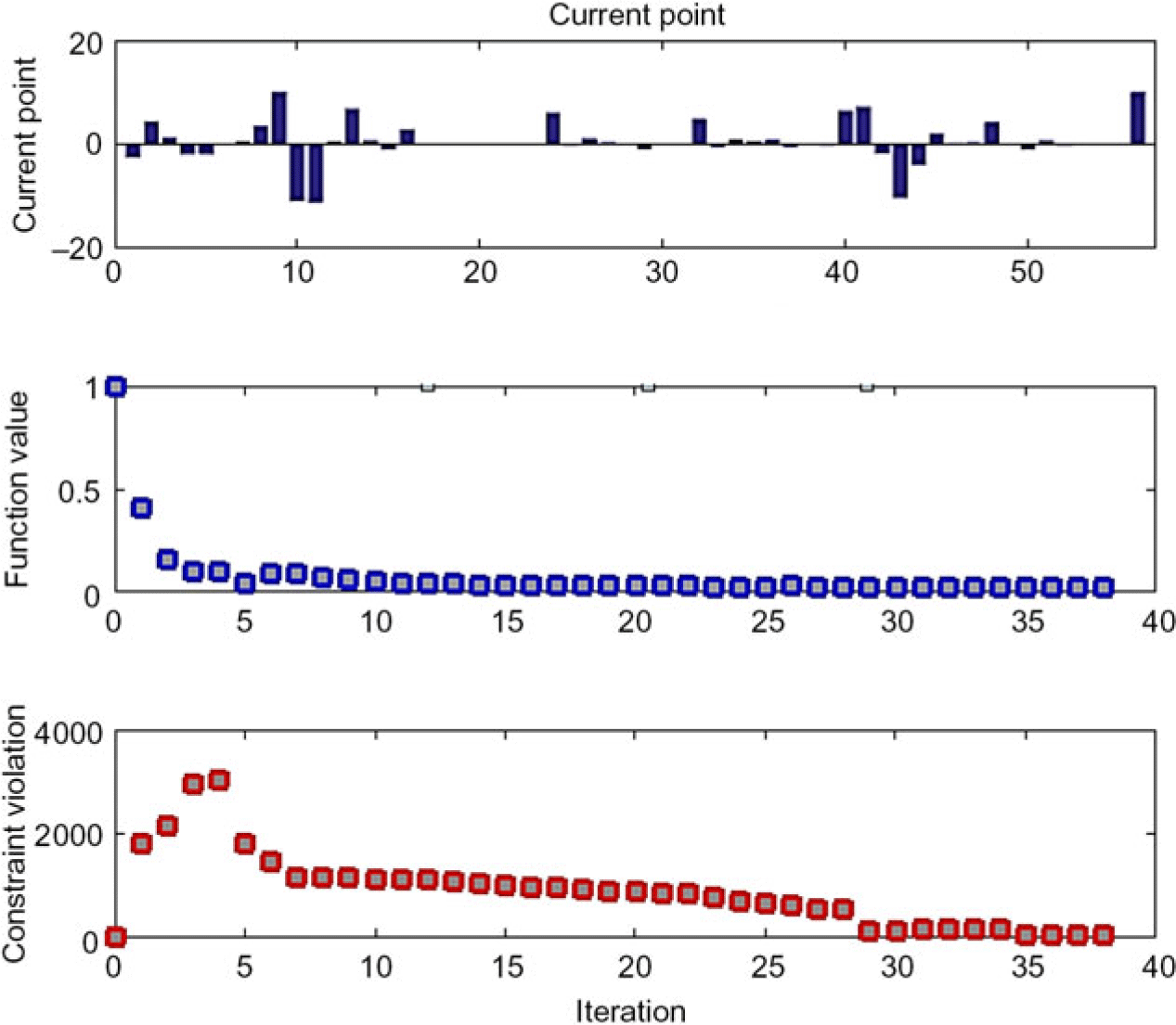
The results have been validated by the acquired experimental results, designed for biomechanical analysis of a healthy human’s walk. The optimization process was performed in two steps using the interior point optimization method in Figures 5 and 6.
First step of the optimization process using Interior Point

Second step of the optimization process using Interior Point

To this end, the vector X, which contains coefficients of Fourier series derived from the approximation of joint angles, was defined. Here, 56 variables were used in the optimization problem.
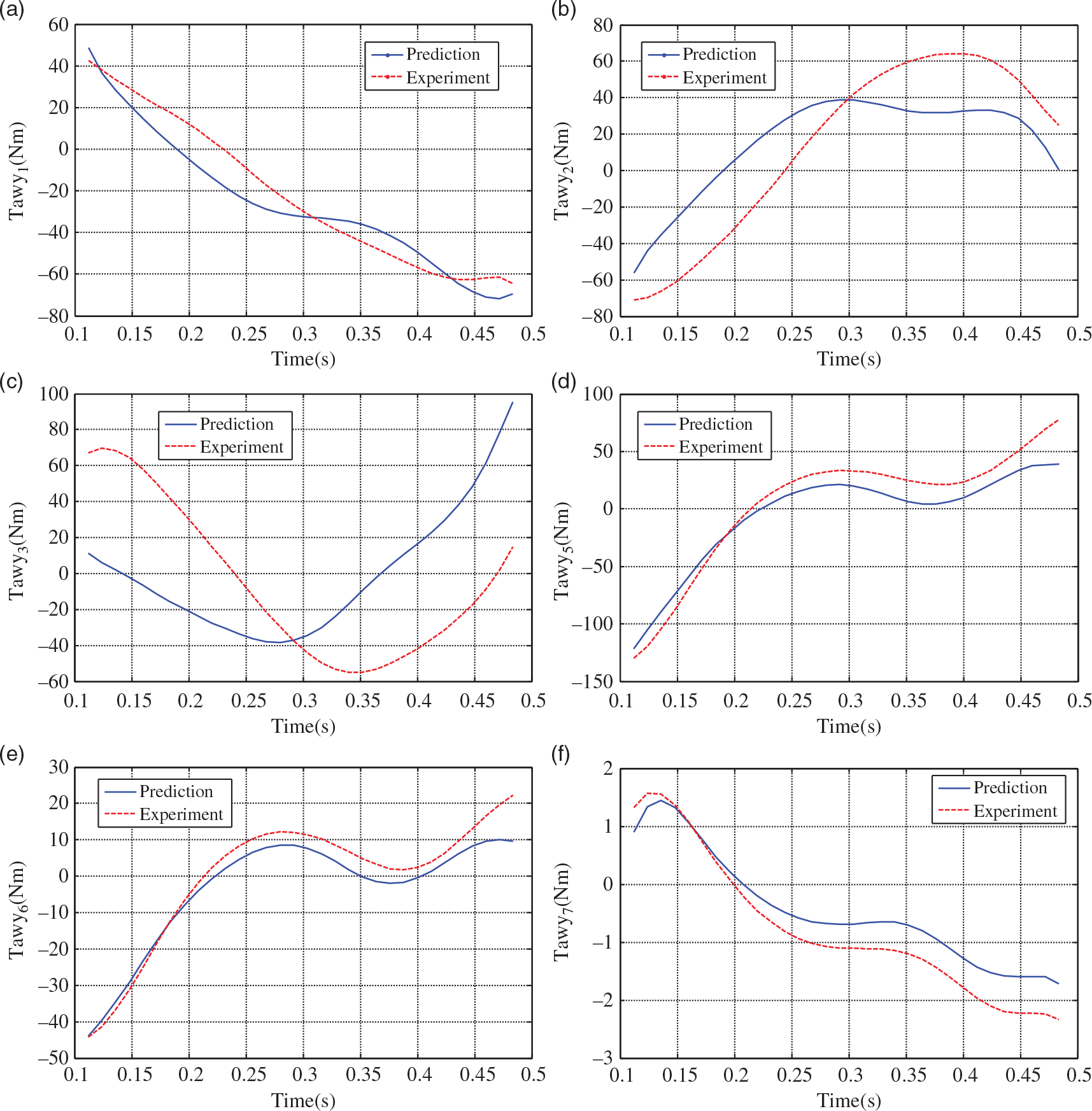
The gait cycle included 981 data among which 376 data were assigned to the single support phase which was extracted and recorded at 0.001-second intervals. The values of the experimental results were used as the initial values for the first step of the optimization process. The output of each stage is used as an input for the next stage. The single support phase (swing) forms 40% of the end of the gait cycle. Human’s single support phase is generally divided into three sub-phases including initial swing which takes about 60%–75% of the stride (one-third of the swing phase). This phase starts when the toe of the swing leg lifts off the ground and then reaches the mid-swing step and ends when the opposite leg is in a static state. This phase, from another point of view, is also called the acceleration phase. In the acceleration phase, the swing leg makes an accelerated forward movement. Then, the leg was thrown into the air affected by the final stage force of the double support phase. The second stage is the mid-swing phase (feet swinging in the air) which ends when the tibia bone of the swinging foot is in the air perpendicular to the ground. This phase takes 73%–87% of the stride. The final phase is the terminal swing phase that takes 87%–100% of the stride and ends when the heel of swinging foot touches the ground. Acceleration of the feet, at this stage, decreases until it slowly touches the ground and that’s why this phase is also called deceleration phase. As shown in Figure 7, all of the optimal joint angles torque follow their experimental pattern perfectly and decreasing trend of first and seventh joint angles shows a decreasing trend of energy consumption over the motion path. The main reasons cause errors to the considered problem attributed to three main categories as below:
1. Error due to marking procedures.
2. Error due to two-dimensional motion assumptions.
3. Error due to the assumption of members being rigorous.
Time history of the joint torques

The following steps are taken to include the effects of these two assumptions on gait kinematics:
a. Joint angles are extracted from the main model (where linkages are not rigid and move in a three-dimensional space) through inverse kinematics using joint positions specified by markers.
b. It is assumed that the length of the linkages is constant (the average length of the member in motion) and that they only move in the sagittal plane (X–Z plane). Further, the positions of the members in the Y-axis are assumed to be completely constant.
c. The horizontal and vertical positions of the joints are calculated using angles obtained from step 1 and applying direct kinematics based on the constant length of members and their movement in the sagittal plane.
d. Deviations from the actual and experimental paths are measured comparing the horizontal and vertical positions of the joints before and after applying the assumptions.
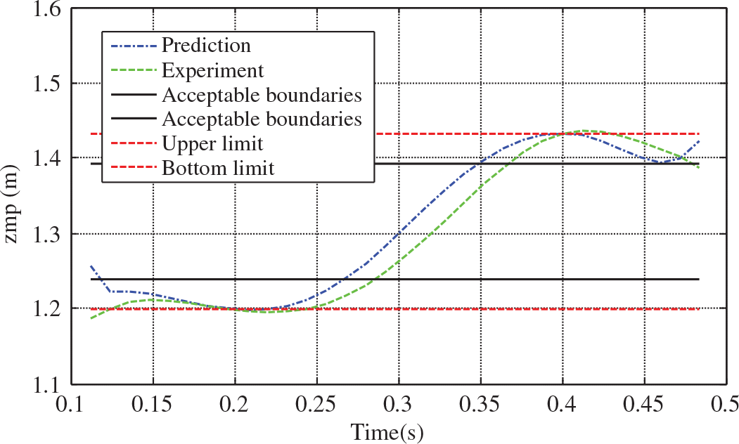
As shown in Figure 8, the position of ZMP is set to be inside the supporting polygon which ensures and demonstrates robot stability over the entire process. To make the problem more similar to human’s walking, the ZMP allowed limit is considered to be slightly greater than this range (with regard to the coverage or lack of coverage of shoes in human feet when walking). This is represented by the dash–dotted lines in Figure 8.
Zero moment point position in the single support phase

Average velocity vs. sum of square torques

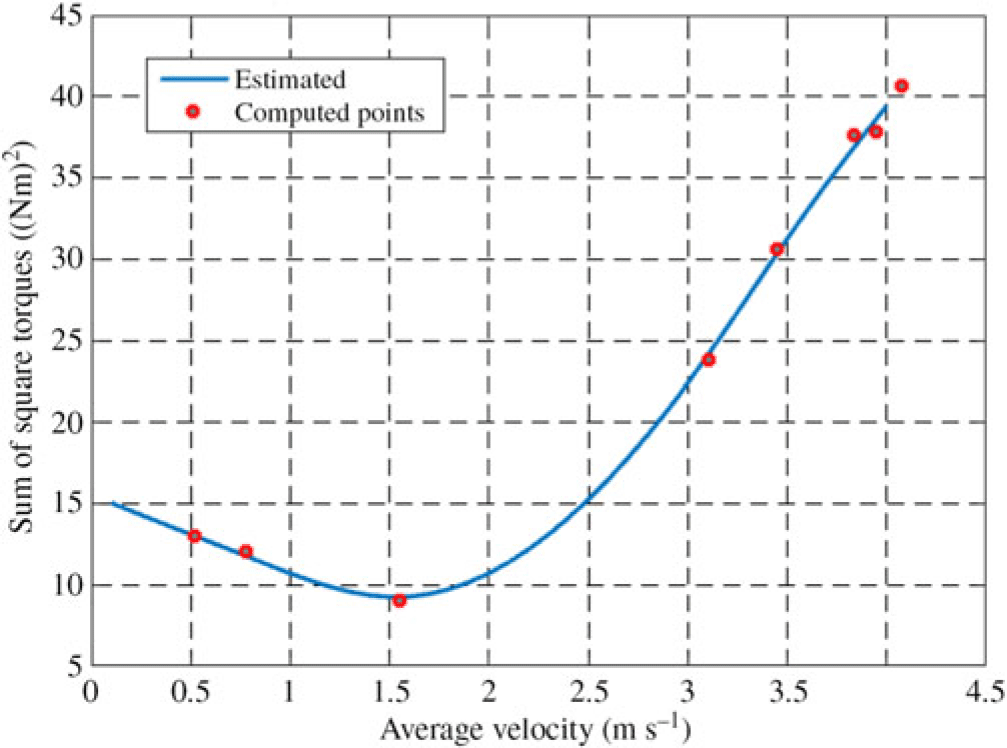
As shown in Figure 9, optimal power consumption was obtained for each average speed. By increasing the average speed of motion, the total optimal energy consumption was decreasing and its minimum value was for speed 1.551 m s−1 and its corresponding value was 9.017 (Nm)2. After this speed, with increasing average speed, optimum energy consumption was increasing significantly. Therefore, the optimum average speed was 1.551 m s−1 which had the lowest energy consumption.
8 Conclusion
Providing maximum stability, increasing power consumption during the motion of a biped robot and trying to reduce energy consumption for this fact affect the stability of the robot and reduce the stability margin. Thus, optimizing these two features simultaneously for a biped robot during the movement is one of the most important goals. In order to make the designed model to look more similar to a human, the trunk torque was not considered to be independent. Furthermore, the verification of the problem was evaluated through the experimental data obtained from a human being selected in this regard. The robot was dynamically analyzed using the Newton–Euler method in the single support phase. Finally, the problem was optimized such that the energy was minimized and the stability reached its maximum during the single support phase and then the human’s correct gait pattern was investigated.
In addition, in this study, the effect of motion average speed on total power consumption was considered and the optimal average speed was achieved 1.551 m s−1 in which the total squared joints torque and resulting energy consumption were at their lowest value.
According to the experiments carried out in this study and with regard to the proposed model, it can be claimed that the robot is capable to walk correctly just like a human and in a way that has the maximum stability and minimum power consumption and is able to create an optimal gait pattern, suitable for anybody else by receiving their anatomical information and employing anthropometric dimensions of their body.
Acknowledgements
This work was financially supported by the Chinese Language and Technology Center of National Taiwan Normal University (NTNU) from The Featured Areas Research Center Program within the framework of the Higher Education Sprout Project by the Ministry of Education (MOE) in Taiwan, and Ministry of Science and Technology, Taiwan, under Grants no. MOST108-2634-F-003-002, MOST108-2634-F-003-003 and MOST108-2634-F-003-004 (administered through Pervasive Artificial Intelligence Research (PAIR) Labs), as well as MOST107-2811-E-003-503. We are grateful to the National Center for High-performance computing for computer time and facilities to conduct this research.
Conflict of interest
The authors confirm that this manuscript and its corresponding research work involve no conflicts of interest.