1. Introduction
A network describes how components are linked to one another. We can represent the components by points (nodes) and the connections by lines (edges) through a mathematical abstraction. The structure comprised of these nodes and edges is called a graph, which has been studied in detail in the field of graph theory (Bollobás Reference Bollobás1998). Network analysis is concerned with the study of graphs as well as the interaction and evolution of the variables of interest on graphs over time and space (Newman Reference Newman2010). The framework developed in network analysis and graph theory can provide insights into how the structure of a network can influence the overall dynamics taking place on the network.
Network analysis and graph theory by nature are very fundamental and generic, which enables them to impact a wide range of applications, including the analysis of biological and social networks, study of traffic flows and design of robust power grids (Newman Reference Newman2010). Biologists and medical scientists use network analysis to determine how electrical signals travel inside the brain and how abnormality in the brain network connections can affect the normal functionality (Duarte-Cavajalino et al. Reference Duarte-Cavajalino, Jahanshad, Lenglet, McMahon, de Zubicaray, Martin, Wright, Thompson and Sapiro2012; Owen et al. Reference Owen, Li, Ziv, Strominger, Gold, Bukhpun, Wakahiro, Friedman, Sherr and Mukherjee2013).
In epidemiology, researchers model the outbreak of diseases on the population network. Locations with high concentrations of population, such as airports, stations, schools and hospitals, can be represented on a network with a large number of connections. The identification of such locations is especially critical when containment measures are designed to control outbreaks of HIV (Morris Reference Morris1993), SARS (Lloyd-Smith et al. Reference Lloyd-Smith, Schreiber, Kopp and Getz2005) and influenza (Glass et al. Reference Glass, Glass, Beyeler and Min2006; Cauchemez et al. Reference Cauchemez, Bhattarai, Marchbanks, Fagan, Ostroff, Ferguson and Swerdlow2011). Each of these diseases has different dynamics and an associated network structure. Once the high-risk groups and areas are identified, network analysis can assist in designing and implementing prevention and combat strategies in the most rapid manner with limited resources (Salathé & Jones Reference Salathé and Jones2010; Robinson, Cohen & Colijn Reference Robinson, Cohen and Colijn2012). Network analysis can also reveal how a group of people are socially connected to one another and examine how subgroups within a population are interlinked in a complex manner (Porter et al. Reference Porter, Mucha, Newman and Warmbrand2005). Moreover, network analysis has been utilized in electrical engineering to determine the voltages and currents associated with electrical circuits via graph representations (Chen Reference Chen2004). In the aforementioned applications of network analysis, the connections between people or elements are highlighted.
In the field of fluid mechanics, extensive studies have been performed to capture the behaviour of complex fluid flow. Lagrangian-based methods, such as vortex methods, allow us to simulate the unsteady fluid flow (Leonard Reference Leonard1980; Cottet & Koumoutsakos Reference Cottet and Koumoutsakos2000). These methods involve modelling of fluid flow with point vortices, vortex sheets, vortex filaments or vortex patches (Saffman Reference Saffman1992; Cottet & Koumoutsakos Reference Cottet and Koumoutsakos2000). Low-order representations of these vortex models (Wang & Eldredge Reference Wang and Eldredge2013; Hemati, Eldredge & Speyer Reference Hemati, Eldredge and Speyer2014) have been proposed in recent years. The evaluation of the velocity field for vortex methods often relies on fast summation methods (Greengard & Rokhlin Reference Greengard and Rokhlin1987) for reduced computational time. The objective of the present study is to extend network analysis and graph theory to discrete point-vortex dynamics.
As the computational approaches for vortex dynamics are being developed, there are also ongoing efforts in flow modelling. Reduced-order models have been utilized successfully to describe unsteady incompressible and compressible flows (Rowley, Colonius & Murray Reference Rowley, Colonius and Murray2004; Noack, Papas & Monkewitz Reference Noack, Papas and Monkewitz2005). One such approach is to utilize Galerkin projection to derive reduced-order models using spatial bases such as the proper orthogonal decomposition (POD) modes (Berkooz, Holmes & Lumley Reference Berkooz, Holmes and Lumley1993; Holmes, Lumley & Berkooz Reference Holmes, Lumley and Berkooz1996). The reduced-order model distils the infinite-dimensional Navier–Stokes equations to model equations with state variables having significantly reduced dimensions. In the present work, we also aim to capture the essential physics of unsteady fluid flow but not by reducing the dimension of the state variable. Instead, we examine the interaction between the elements of the state variables and sparsify the interactions utilizing a network-theoretic approach. We refer to the dynamical model based on sparsifying the interactions as sparsified dynamics in this paper.
In the present work, we consider representing vortices with nodes and the interactions amongst the vortices with edges. By utilizing the network-theoretic framework to study vortex dynamics, we highlight the connections (edges) that the vortices have in the flow field. Such analysis emphasizes how a collection of vortices influence each other through a causal point of view on a network structure. We believe that the present study can provide an alternative tool to analyse how vortices or flow structures interact in the flow field and support the development of interaction-based models to capture unsteady vortex dynamics. Furthermore, we consider the use of graph sparsification as a tool for sparsifying the interaction between the point vortices. These models keep the nodes intact and reduce the number of edges, maintaining the dimensionality of the original system, unlike reduced-order models. The removal of edges can drastically reduce computational cost to model the full dynamical behaviour, sharing the same spirit as reduced-order models.
In what follows, we first introduce network analysis and graph theory briefly in § 2. We introduce the notion of graph sparsification in § 3. We then consider the use of network analysis on discrete vortex dynamics and derive sparsified models in § 4. Some comments are offered on the difference between the sparsified-dynamics model and the reduced-order model. Concluding remarks are offered in § 5.
2. Network-theoretic framework
A network is defined by a collection of vertices joined by edges. These edges form the bonds that connect the vertices or the various entities of the system together. The edges can be associated with weights describing the importance of the connections between the vertices. Such a graph is called a weighted graph. If the edges of the graph have an associated directivity (i.e. one vertex influences the other but not vice versa), the graph is called a directed graph. If a vertex influences itself, a self-loop edge (edge reconnected to itself) can represent such an effect. Any undirected graph
 $G$
can be described by a set of vertices
 $V=\{v_{1},v_{2},\dots ,v_{N}\}$
, a set of edges
 $E$
and a set of weights
 $w$
associated with the edges, i.e.
 $G=\{V,E,w\}$
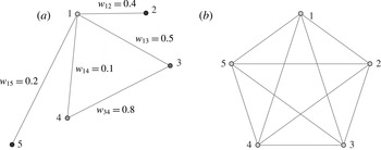
(Chung Reference Chung1997; Newman Reference Newman2010). An example of a weighted graph is shown in figure 1(a) with the weights associated with the edges displayed. A complete graph
 $K_{N}$
with
 $N=5$
, shown in figure 1(b), has all the vertices connected to each other. In other words, this graph has
 $N$
vertices with the complete set of possible
 $N(N-1)/2$
edges without any self-loops. We later use a weighted version of the complete graph to describe the interactions amongst a set of discrete point vortices in the context of fluid dynamics.
(a) An example weighted graph and (b) a complete graph
 $K_{5}$
.

Network connections can be summarized by the adjacency matrix
 $\unicode[STIX]{x1D63C}_{G}\in \mathbb{R}^{N\times N}$
, which is given by
 $$\begin{eqnarray}[\unicode[STIX]{x1D608}_{G}]_{ij}=\left\{\begin{array}{@{}ll@{}}w_{ij}\quad & \text{if }(i,j)\in E\\ 0\quad & \text{otherwise}.\end{array}\right.\end{eqnarray}$$
In an unweighted graph, the weight is set to unity if
 $(i,j)\in E$
. The diagonal entries of the adjacency matrix relate to the weight of the self-connecting (loops) edges. The adjacency matrix of an undirected graph is symmetric. The degree
 $k_{i}$
of a vertex
 $i$
represents the summation of the weights of the edges connected to it, given by
 $k_{i}=\sum _{j=1}^{N}[\unicode[STIX]{x1D608}_{G}]_{ij}$
. The adjacency matrices for an example graph
 $\unicode[STIX]{x1D63C}_{G}$
and the complete graph
 $\unicode[STIX]{x1D63C}_{K_{5}}$
shown in figure 1 are given by
 $$\begin{eqnarray}\unicode[STIX]{x1D63C}_{G}=\left(\begin{array}{@{}ccccc@{}}0 & 0.4 & 0.5 & 0.1 & 0.2\\ 0.4 & 0 & 0 & 0 & 0\\ 0.5 & 0 & 0 & 0.8 & 0\\ 0.1 & 0 & 0.8 & 0 & 0\\ 0.2 & 0 & 0 & 0 & 0\end{array}\right)\quad \text{and}\quad \unicode[STIX]{x1D63C}_{K_{5}}=\left(\begin{array}{@{}ccccc@{}}0 & 1 & 1 & 1 & 1\\ 1 & 0 & 1 & 1 & 1\\ 1 & 1 & 0 & 1 & 1\\ 1 & 1 & 1 & 0 & 1\\ 1 & 1 & 1 & 1 & 0\end{array}\right),\end{eqnarray}$$
where
 $G$
is a weighted graph and
 $K_{5}$
is an unweighted complete graph.
Another important matrix in graph theory is the graph Laplacian matrix
 $\unicode[STIX]{x1D647}_{G}\in \mathbb{R}^{N\times N}$
, which is given by
 $$\begin{eqnarray}[\unicode[STIX]{x1D613}_{G}]_{ij}=\left\{\begin{array}{@{}ll@{}}k_{i}\quad & \text{if }(i,j)\in E~\text{and}~(i=j)\\ -w_{ij}\quad & \text{if }(i,j)\in E~\text{and}~(i\neq j)\\ 0\quad & \text{otherwise}.\end{array}\right.\end{eqnarray}$$
The graph Laplacian matrix can also be deduced from the adjacency matrix,
 $\unicode[STIX]{x1D647}_{G}=\unicode[STIX]{x1D63F}_{G}-\unicode[STIX]{x1D63C}_{G}$
, where
 $\unicode[STIX]{x1D63F}_{G}\in \mathbb{R}^{N\times N}$
is a diagonal matrix with elements equal to degrees of vertices,
 $\unicode[STIX]{x1D63F}_{G}=\text{diag}([k_{i}]_{i=1}^{N})$
. For undirected networks, it is symmetric and positive semidefinite (singular). This Laplacian matrix is a discrete analogue of the negative continuous Laplacian operator (
 $-{\rm\nabla}^{2}$
) and is also called the discrete Laplacian. It is naturally defined by its quadratic form. If we have a linear system of the form
 $\unicode[STIX]{x1D647}_{G}\boldsymbol{x}=\boldsymbol{b}$
, for the vector
 $\boldsymbol{x}\in \mathbb{R}^{N}$
, the Laplacian quadratic form of a weighted graph
 $G$
is given by (Mohar Reference Mohar, Alavi, Chartrand, Ollermann and Schwenk1991)
 $$\begin{eqnarray}\boldsymbol{x}^{\text{T}}\unicode[STIX]{x1D647}_{G}\boldsymbol{x}=\mathop{\sum }_{(i,j)\in E}w_{ij}(x_{i}-x_{j})^{2}.\end{eqnarray}$$
The discrete Laplacian is a smoothness indicator of
 $\boldsymbol{x}$
over the edges in
 $G$
. The Laplacian quadratic form becomes large as
 $\boldsymbol{x}$
jumps over the edges of
 $G$
. The definitions of adjacency matrix and graph Laplacian form the building blocks of the graph-theoretic framework. The Laplacian quadratic form will be used below to introduce the notion of spectral similarity of graphs and graph sparsification.
3. Graph sparsification
The sparse approximation of dense graphs can provide numerous benefits for numerical computation. Graph sparsification is useful for the design of computationally efficient algorithms and helps in identifying representative edges and associated weights (Spielman & Teng Reference Spielman and Teng2011). Graph similarity, which forms the basis for graph sparsification, can be derived in a number of ways depending on the desired similarity properties. Distance similarity of graphs (Peleg & Ullman Reference Peleg and Ullman1989) can be achieved by sparse graphs called spanners that keep the same shortest-path distance between each pair of vertices as in the original graph, while cut similarity (Benczúr & Karger Reference Benczúr and Karger1996) can be achieved by maintaining the weight of the edges leaving a set of vertices of the sparse graph to be the same as that of the original graph. A much stronger notion of similarity referred to as spectral similarity was introduced by Spielman & Teng (Reference Spielman and Teng2011). Spectral similarity is closely tied to the Laplacian quadratic form of the graphs as defined by (2.4). The concept of spectral similarity directly leads to spectral sparsification of graphs; that is to create sparse graphs that are spectrally similar to the original graphs.
3.1. Spectral sparsification
Spectral sparsification is a more general abstraction than cut sparsifiers and maintains spectral similarity between the sparsified and original graphs. In particular, spectral sparsification can remove some of the edges in the graph, while maintaining similar adjacency and Laplacian eigenspectra. One of the key features of spectral sparsification is that it keeps the sum of the weights leaving the vertex of a graph constant. A spectral sparsifier is a subgraph of the original graph whose Laplacian quadratic form is approximately the same as the original graph (Spielman & Teng Reference Spielman and Teng2011).
Sparsification involves the creation of a sparse graph
 $G_{S}$
from the original graph
 $G$
based on an approximation order of
 ${\it\epsilon}$
. The quadratic form induced by the graph Laplacian of
 $G$
is maintained up to a multiplicative
 $(1\pm {\it\epsilon})$
factor by spectral sparsification (Kelner & Levin Reference Kelner and Levin2011). Thus, the sparse graph
 $G_{S}$
is a
 $(1\pm {\it\epsilon})$
-spectral approximation of
 $G$
. The approximation order
 ${\it\epsilon}$
can vary from zero to unity. The approximation with
 ${\it\epsilon}=0$
indicates that
 $G_{S}$
is same as the original graph
 $G$
and none of the edges are sparsified, while
 ${\it\epsilon}=1$
relaxes the quadratic form induced by the sparse graph to within twice that induced by the original graph. An approximation of
 ${\it\epsilon}=1$
leads to a heavily sparsified graph. Denoting the Laplacian matrices of
 $G$
and
 $G_{S}$
by
 $\unicode[STIX]{x1D647}_{G}$
and
 $\unicode[STIX]{x1D647}_{G_{S}}$
respectively, the spectrally sparsified Laplacian satisfies
 $$\begin{eqnarray}(1-{\it\epsilon})\boldsymbol{x}^{\text{T}}\unicode[STIX]{x1D647}_{G}\boldsymbol{x}\leqslant \boldsymbol{x}^{\text{T}}\unicode[STIX]{x1D647}_{G_{S}}\boldsymbol{x}\leqslant (1+{\it\epsilon})\boldsymbol{x}^{\text{T}}\unicode[STIX]{x1D647}_{G}\boldsymbol{x}\end{eqnarray}$$
at least with probability
 $1/2$
with large
 $N$
for all
 $\boldsymbol{x}\in \mathbb{R}^{N}$
(Spielman & Srivastava Reference Spielman and Srivastava2011). For the example problem considered later, these bounds are much tighter. This tells us that
 $\unicode[STIX]{x1D647}_{G_{S}}$
holds eigenvalues similar to those of
 $\unicode[STIX]{x1D647}_{G}$
. These spectrally similar sparse graphs are found using the spectral sparsification algorithm based on sampling by effective resistance discussed below.
Before we discuss how a graph can be sparsified, let us first follow the works of Bollobás (Reference Bollobás1998) and Srivastava (Reference Srivastava2010) to establish an analogy of a graph to an electrical circuit. If the entire graph is viewed as a resistive circuit, we can define a resistance on the individual edges
 $e=(i,j)$
of the graph. According to Thomson’s principle, the potentials and currents in a resistive circuit distribute themselves so as to minimize the total energy in the network (Bollobás Reference Bollobás1998). This energy-minimization principle leads to the concept of effective resistance.
The effective resistance between vertices
 $i$
and
 $j$
is the potential difference induced between them when a unit current is injected at one vertex and extracted at the other (Bollobás Reference Bollobás1998; Srivastava Reference Srivastava2010). The effective graph resistance (also called the resistance distance) is the sum of the effective resistances over all the pairs of vertices in the graph
 $G$
(Klein & Randić Reference Klein and Randić1993; Ellens et al.
Reference Ellens, Spieksma, Van Mieghem, Jamakovic and Kooij2011). Rayleigh’s monotonicity law states that pairwise effective resistance is a non-increasing function of the edge weights (Mieghem Reference Mieghem2011).
In order to obtain an expression of the effective resistance for graph sparsification, we orient the edges of the original weighted undirected graph
 $G$
with
 $N$
vertices and
 $M$
edges. We can represent any directed graph by a signed edge (
 $e$
)–vertex (
 $v$
) incidence matrix
 $\unicode[STIX]{x1D63D}_{G}\in \mathbb{R}^{M\times N}$
given by
 $$\begin{eqnarray}[\unicode[STIX]{x1D609}_{G}]_{ev}=\left\{\begin{array}{@{}ll@{}}1\quad & \text{if }e\in E~\text{and}~v~\text{is the head of }e\\ -1\quad & \text{if }e\in E~\text{and}~v~\text{is the tail of }e\\ 0\quad & \text{otherwise}.\end{array}\right.\end{eqnarray}$$
The row of
 $\unicode[STIX]{x1D63D}_{G}$
corresponding to an edge
 $e=(i,j)$
is given by
 $(\,\boldsymbol{p}_{i}-\boldsymbol{q}_{j})$
, where
 $\boldsymbol{p}_{i}$
and
 $\boldsymbol{q}_{j}$
are elementary unit vectors in the
 $i$
and
 $j$
directions respectively. If the edge weights of the graph are represented in a diagonal matrix given by
 $\unicode[STIX]{x1D63E}_{G}\in \mathbb{R}^{M\times M}$
, we can express the Laplacian matrix based on the incidence matrix as
 $$\begin{eqnarray}\unicode[STIX]{x1D647}_{G}=\unicode[STIX]{x1D63D}_{G}^{\text{T}}\unicode[STIX]{x1D63E}_{G}\unicode[STIX]{x1D63D}_{G}=\mathop{\sum }_{i,j\in E}w_{ij}(\,\boldsymbol{p}_{i}-\boldsymbol{q}_{j})(\,\boldsymbol{p}_{i}-\boldsymbol{q}_{j})^{\text{T}}.\end{eqnarray}$$
The above relation holds true only for undirected graphs. The incidence matrix
 $\unicode[STIX]{x1D63D}_{G}$
and the diagonal matrix
 $\unicode[STIX]{x1D63E}_{G}$
for the example graph shown in figure 1(a) are given by
 $$\begin{eqnarray}\unicode[STIX]{x1D63D}_{G}=\left(\begin{array}{@{}ccccc@{}}1 & -1 & 0 & 0 & 0\\ 1 & 0 & -1 & 0 & 0\\ 1 & 0 & 0 & -1 & 0\\ 0 & 0 & 1 & -1 & 0\\ 1 & 0 & 0 & 0 & -1\end{array}\right)\quad \text{and}\quad \unicode[STIX]{x1D63E}_{G}=\left(\begin{array}{@{}ccccc@{}}0.4 & 0 & 0 & 0 & 0\\ 0 & 0.5 & 0 & 0 & 0\\ 0 & 0 & 0.1 & 0 & 0\\ 0 & 0 & 0 & 0.8 & 0\\ 0 & 0 & 0 & 0 & 0.2\end{array}\right).\end{eqnarray}$$
For undirected graphs, each edge is counted only once in the incidence matrix and the convention for head and tail of an edge can be fixed arbitrarily. Here, for edge
 $e=(1,2)$
of the example graph shown in figure 1(a), the head and tail are considered to be vertices 1 and 2 respectively. The corresponding elementary unit vectors for the edge are given by
 $\boldsymbol{p}_{1}=(1,0,0,0,0)$
and
 $\boldsymbol{q}_{2}=(0,1,0,0,0)$
, which is apparent from the first row of
 $\unicode[STIX]{x1D63D}_{G}$
being
 $\boldsymbol{p}_{1}-\boldsymbol{q}_{2}$
.
For an edge corresponding to
 $e=(i,j)$
, the unit current is injected at vertex
 $i$
and extracted at vertex
 $j$
. Thus, we set the electrical current across the edge to be
 $(\,\boldsymbol{p}_{i}-\boldsymbol{q}_{j})$
. The potential induced by this current at the vertices is given by
 $\unicode[STIX]{x1D647}_{G}^{+}(\,\boldsymbol{p}_{i}-\boldsymbol{q}_{j})$
, where
 $\unicode[STIX]{x1D647}_{G}^{+}$
is the Moore–Penrose pseudoinverse of the Laplacian matrix
 $\unicode[STIX]{x1D647}_{G}$
(Srivastava Reference Srivastava2010). The potential difference across edge
 $e=(i,j)$
is then given by
 $(\,\boldsymbol{p}_{i}-\boldsymbol{q}_{j})^{\text{T}}\unicode[STIX]{x1D647}_{G}^{+}(\,\boldsymbol{p}_{i}-\boldsymbol{q}_{j})$
. Thus, for unit current, the effective resistance across edge
 $e=(i,j)$
, which corresponds to the potential difference, can be expressed as
 $$\begin{eqnarray}[R_{e}]_{ij}=(\,\boldsymbol{p}_{i}-\boldsymbol{q}_{j})^{\text{T}}\unicode[STIX]{x1D647}_{G}^{+}(\,\boldsymbol{p}_{i}-\boldsymbol{q}_{j}).\end{eqnarray}$$
The above expression is used for computing the effective resistance of the edges of the graph. The sparsification of the original graph
 $G=\{V,E,w\}$
is performed with the algorithm
 $\mathtt{Sparsify}$
(Spielman & Srivastava Reference Spielman and Srivastava2011) to produce a sparse graph
 $G_{S}=\{V,\widetilde{E},\widetilde{w}\}$
, where
 $\widetilde{w}$
are the weights corresponding to the sparse graph
 $G_{S}$
. This algorithm is based on the concept of effective resistance and yields a
 $(1+{\it\epsilon})$
sparse graph
 $G_{S}$
. This sparse graph contains a reduced number of
 $O(N\log (N)/{\it\epsilon}^{2})$
of edges. The procedure for sparsification
 $G_{S}=\mathtt{Sparsify}(G)$
is summarized below.
3.2. Summary of algorithm
We first create a list of the edges
 $E$
with the associated weights of the original graph
 $G$
. The adjacency and Laplacian matrices of the graph
 $G$
are constructed from (2.1) and (2.3). The Moore–Penrose pseudoinverse of the Laplacian matrix
 $\unicode[STIX]{x1D647}_{G}^{+}$
is then computed. For each edge in the edge list, the elementary unit vectors
 $\boldsymbol{p}_{i}$
and
 $\boldsymbol{q}_{j}$
and edge weights
 $w_{e}$
are obtained. Next, the effective resistance
 $[R_{e}]_{ij}$
corresponding to each edge is computed from (3.5).
A random edge
 $e=(i,j)$
from the edge list of graph
 $G$
is chosen with probability
 $p_{e}$
proportional to
 $w_{e}[R_{e}]_{ij}$
. The edge
 $e$
is added to the sparse graph
 $G_{S}$
with the weight given by
 $\widetilde{w}_{e}=w_{e}/qp_{e}$
, where
 $q=8N\log _{2}(N)/{\it\epsilon}^{2}$
. We take an integer(
 $q$
) number of samples independently without replacement and sum the weights if an edge is chosen more than once. The resulting graph becomes the sparsified graph
 $G_{S}$
that satisfies equation (3.1) with eigenvalues similar to those of
 $G$
.
After the random sampling procedure, a sparsified adjacency matrix
 $\unicode[STIX]{x1D63C}_{G_{S}}$
is obtained. For convenience, we define the ratio of the sparsified and original adjacency matrix weights as
 $W_{ij}$
,
 $$\begin{eqnarray}W_{ij}\equiv \left\{\begin{array}{@{}ll@{}}\widetilde{w}_{ij}/w_{ij}\quad & \text{if }(i,j)\in \widetilde{E}\\ 0\quad & \text{otherwise}.\end{array}\right.\end{eqnarray}$$
This sparsification factor
 $W_{ij}$
is related to the probability of an edge
 $e=(i,j)$
of graph
 $G$
being sampled. The edges of the original graph that are not sampled during the random sampling procedure have zero weights in the sparsified graph. These edges are cut during sparsification. The spectral sparsification procedure also redistributes the weights of the cut edges among the other edges of the sparsified graph. Thus, cutting of graph edges is compensated by redistribution of the weights to preserve the spectral properties of the original graph.
The spectral sparsification algorithm described above produces a (
 $1\pm {\it\epsilon}$
) expander graph, i.e. a sparsifier with strong connectivity properties when
 ${\it\epsilon}\geqslant 1/\sqrt{N}$
, where
 $N$
is the number of vertices (Spielman & Srivastava Reference Spielman and Srivastava2011). With the concept of graphs and spectral sparsification now discussed, we consider the application of network analysis to discrete vortex dynamics in the next section.
4. Applications to discrete vortex dynamics
We apply network analysis to study the dynamics of a collection of point vortices (Saffman Reference Saffman1992; Newton Reference Newton2001). In the present work, the flow is assumed to be two-dimensional, incompressible and inviscid. The spatial domain
 $\mathscr{D}$
is taken to be infinitely large and the position of the vortices in the flow field is denoted by
 $\boldsymbol{r}=(x,y)\in \mathscr{D}$
. We consider a collection of
 $N$
vortices to be in the domain
 $\mathscr{D}$
, resulting in the vorticity field of
 $$\begin{eqnarray}{\it\omega}(\boldsymbol{r})=\mathop{\sum }_{j=1}^{N}\frac{{\it\kappa}_{j}}{2{\rm\pi}}{\it\delta}(\boldsymbol{r}-\boldsymbol{r}_{j}),\end{eqnarray}$$
where
 ${\it\kappa}_{j}$
and
 $\boldsymbol{r}_{j}$
are the strength (circulation) and position of the
 $j$
th vortex respectively, and
 ${\it\delta}(\cdot )$
is the Dirac delta function. The motion of the vortices is described by the Biot–Savart law,
 $$\begin{eqnarray}\frac{\text{d}\boldsymbol{r}_{\boldsymbol{i}}}{\text{d}t}=\mathop{\sum }_{\begin{array}{@{}c@{}}j=1\\ j\neq i\end{array}}^{N}\frac{{\it\kappa}_{j}}{2{\rm\pi}}\frac{\hat{\boldsymbol{k}}\times (\boldsymbol{r}_{i}-\boldsymbol{r}_{j})}{|\boldsymbol{r}_{i}-\boldsymbol{r}_{j}|^{2}},\end{eqnarray}$$
where
 $\hat{\boldsymbol{k}}$
is the out-of-plane unit normal vector. To determine the trajectories of the vortices, we numerically integrate the above equation. This equation is the basis of the discrete vortex methods that are used to simulate unsteady vortical flows in place of discretizing the two-dimensional Euler equations.
The objective of the present work is to describe the interactions amongst a set of point vortices with graph theory and network analysis. The dynamics of the vortices will be modelled on a sparsified graph in place of the full (complete) graph to derive a sparsified model that accurately captures the motion of the vortices while conserving physical properties, such as circulation, Hamiltonian, as well as linear and angular impulse.
4.1. Representing vortex interactions on a graph
A vortex is advected by the induced velocity from the other vortices and not by its own velocity, as seen in (4.2). Each vortex is influenced by all other vortices, which means that each and every vortex has a connection to all other vortices without any self-loops. Thus, the discrete system of
 $N$
point vortices can be represented by a weighted complete graph,
 $K_{N}$
. The vertices or nodes of the graph represent the discrete point vortices and the edge weights represent the strength of the connections between them.
The motion of the point vortices is influenced by the strengths (circulation) of the individual point vortices and the distances between them. The point vortices exert stronger influence on each other when they are closer. Moreover, a vortex with higher strength has more ability to influence the surrounding vortices compared with that with lower strength. We assign the weight for the interaction between two vortices to be dependent on the characteristic vortex-induced velocity based on the strengths of the two vortices and the distance between them. Thus, this implies that the edge weight for the vortex network should be proportional to
 ${\it\kappa}/r$
, where
 ${\it\kappa}$
is the characteristic strength of the two vortices and
 $r$
is the distance between them within the network.
The distance between the vortices is dependent on the location of the two point vortices
 $|\boldsymbol{r}_{i}-\boldsymbol{r}_{j}|$
, and the characteristic strength can be established by considering their geometric mean
 $\sqrt{|{\it\kappa}_{i}{\it\kappa}_{j}|}$
. This choice makes the adjacency matrix symmetric, which allows the use of the spectral sparsification algorithm discussed in § 3.1. Therefore, the adjacency matrix for the graph representation of a set of point vortices can be defined as
 $$\begin{eqnarray}[\unicode[STIX]{x1D608}_{G}]_{ij}=\left\{\begin{array}{@{}ll@{}}\displaystyle \frac{\sqrt{|{\it\kappa}_{i}{\it\kappa}_{j}|}}{|\boldsymbol{r}_{i}-\boldsymbol{r}_{j}|}\quad & \text{if }(i,j)\in E\text{ and }i\neq j\\ 0\quad & \text{otherwise}.\end{array}\right.\end{eqnarray}$$
It should be noted that the diagonal elements of the adjacency matrix are zero as the self-induced velocity components are zero. This translates to the graph not having any self-loops. The interaction between the system of discrete point vortices represented on a complete graph can be sparsified for deriving the sparse vortex interaction model.
In addition to considering the geometric mean of the circulation for the weights, the algebraic mean of the circulation was also considered. The computation using the algebraic mean (i.e.
 $((|{\it\kappa}_{i}|+|{\it\kappa}_{j}|)/2)/|\boldsymbol{r}_{i}-\boldsymbol{r}_{j}|$
) for the weights performed similarly to that with the above geometric mean. While we show that the geometric mean sufficiently captures the vortex interaction, there may be some room for optimizing the choice of weights. In what follows we utilize the geometric mean in (4.3) for the network weight.
4.2. Sparsification of vortex interactions
In this section, we construct a sparsified representation of the vortex interactions by sparsifying and redistributing the weights of the connections between the point vortices as discussed in § 3.1. We consider a configuration of
 $N$
point vortices in
 $n_{c}$
clusters. This set-up allows us to examine the effect of sparsification on a cluster of vortices. The edge weights represented in the adjacency matrix are given by (4.3).
Let us first consider a collection of
 $N=100$
point vortices with
 $n_{c}=5$
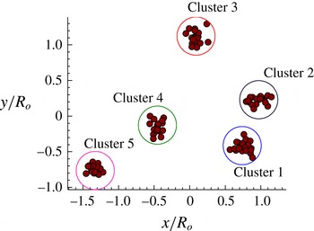
, with each cluster containing 20 vortices. The clusters in this set-up can be clearly identified by the use of graph clustering algorithms. An algorithm that maximizes modularity (Newman Reference Newman2004) can be utilized for the identification of clusters. One could also use
 $k$
-means for cluster identification, similarly to the work performed by Kaiser et al. (Reference Kaiser, Noack, Cordier, Spohn, Segond, Abel, Daviller and Niven2014). The point vortices in a particular cluster are given a normal distribution in space with a radial standard deviation of
 ${\it\sigma}_{r}=0.2$
. The strengths of the point vortices,
 ${\it\kappa}_{i}$
, within the individual clusters have a normal distribution with a mean of
 $\bar{{\it\kappa}}=0.1$
and a standard deviation of
 ${\it\sigma}_{{\it\kappa}}=0.01$
. The set-up for this configuration is shown in figure 2. The positions of the clusters are normalized by the average radial distance of the centroid of the clusters from the geometric centre of the system (
 $R_{o}$
).
The spatial arrangement of
 $N=100$
point vortices with five clusters.

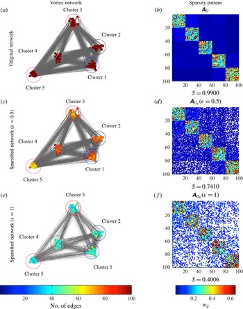
The original point-vortex distribution modelled as a complete graph is shown in figure 3(a). The colours of the point vortices (network vertices) indicate their unweighted degree (number of edge connections). As the original graph here is a complete graph
 $K_{N}$
, each vortex is connected to every other vortex. Thus, the unweighted degree of each vortex in this example is
 $N-1=99$
. The sparsity pattern of the adjacency matrix for the complete graph
 $\unicode[STIX]{x1D63C}_{K_{N}}$
is shown in figure 3(b). We also note in the figure the sparsity index
 $S$
, defined as
 $S\equiv n_{\mathit{non\text{-}zero}}/N^{2}$
, where
 $n_{\mathit{non\text{-}zero}}$
is the number of non-zero weights in the adjacency matrix and
 $N$
is the number of vortices. As the diagonal elements of the adjacency matrix have zero weights,
 $n_{\mathit{non\text{-}zero}}=N(N-1)$
for the complete graph. For
 $N=100$
, a sparsity index of
 $S=0.99$
is obtained for the original graph.
Original and sparsified graphs and their respective sparsity patterns of the adjacency matrix for
 $N=100$
vortices. The colour of the nodes of the vortex network represents the unweighted connections (number of connected edges) of the individual point vortices. The colour in the sparsity patterns of the adjacency matrix indicates the adjacency weights
 $w_{ij}$
for the original graph
 $\unicode[STIX]{x1D63C}_{G}$
and
 $\widetilde{w}_{ij}$
for the sparse graphs
 $\unicode[STIX]{x1D63C}_{G_{S}}$
. The empty white spaces indicate sparsity in the adjacency matrix. The sparsity index is
 $S\equiv n_{\mathit{non\text{-}zero}}/N^{2}$
, where
 $n_{\mathit{non\text{-}zero}}$
is the number of non-zero weights (elements) in the adjacency matrix and
 $N$
is the number of vortices. The coloured circles in the vortex network represent the individual cluster groups.

We now perform spectral sparsification on the original graph (
 $G=K_{N}$
) using the algorithm
 $G_{S}=\mathtt{Sparsify}(G)$
described in § 3.1 to obtain the spectrally similar sparse representations of the complete graph based on approximation order
 ${\it\epsilon}$
. The corresponding adjacency matrix,
 $\unicode[STIX]{x1D63C}_{G_{S}}$
can also be found. The vortex network for the sparse graph and the sparsity pattern of
 $\unicode[STIX]{x1D63C}_{G_{S}}$
corresponding to an approximation order of
 ${\it\epsilon}=0.5$
are shown in figure 3(c,d). We observe that the number of edges (connections) between the vortices in clusters 3 and 5 is reduced. Because the weights of the adjacency matrix are inversely proportional to the distance between the vortices, a large number of edges between the vortices of the clusters with larger distances are cut during sparsification. The sparsity index decreases from
 $S=0.99$
for the original complete graph to
 $S=0.741$
for the sparse graph (
 ${\it\epsilon}=0.5$
), reducing the number of connections by approximately 25 %.
The vortex network and sparsity patterns for an approximation order of
 ${\it\epsilon}=1$
are shown in figure 3(e,f). We observe a dense representation of the connections between the clusters 1 and 2. Thus, the proximity in clusters is identified in both the network structure and the sparsity patterns. Moreover, we realize from the sparsity patterns that the connections between the vortices in a particular cluster are maintained, while the majority of the inter-cluster ties are cut, resulting in a sparse graph. The number of connections in the sparse graph for
 ${\it\epsilon}=1$
is reduced dramatically by nearly 60 %, with
 $S=0.4006$
.
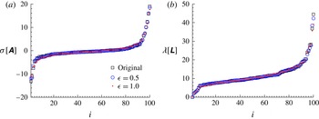
For weighted graphs, the effective resistance is computed in such as way as to maintain spectral similarity. The eigenspectra (
 ${\it\sigma}$
and
 ${\it\lambda}$
) of the adjacency and Laplacian matrices for the sparse and original graphs are compared in figure 4. We observe from figure 4 that the spectra of the sparse and original configurations are in good agreement, as expected. The second smallest eigenvalue of the Laplacian matrix represents the spectral gap or algebraic connectivity of the graph, i.e. vertices connected by at least a single path (Newman Reference Newman2010). As observed from figure 4, the spectral gap is greater than zero for the original and sparse graphs, indicating that the graph is connected. Thus, sparsification preserves the connectivity properties of the original graph. The sparsified graphs slightly underpredict the maximum eigenvalues of the adjacency and Laplacian matrices compared with the original graph. The preservation of spectral properties is attractive if the sparsified network is to be used to describe the dynamics of the vortices. We expect the overall motion of the vortices to remain similar with sparsified representations of the vortex interactions.
Eigenvalue spectra of the adjacency (a) and Laplacian (b) matrices of the sparsified graphs with
 ${\it\epsilon}=0.5$
and 1 in comparison with the original graph.

Sparsification helps to identify the individual clusters by creating subgraphs within a graph where the density of the edges between vertices is much greater than that outside it. The spectral sparsification procedure leads to a reduction in the number of edges to
 $O(N\log (N)/{\it\epsilon}^{2})$
for large
 $N$
. We examine the performance of spectral sparsification on the present example for an increase in the total number of vortices. As in the example that was previously considered, we maintain a constant number of clusters
 $n_{c}=5$
but increase the number of vortices in each cluster
 $N/n_{c}$
. The sparsity patterns of the adjacency matrix for
 $N=500$
and 2000 with approximation order
 ${\it\epsilon}=1$
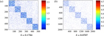
are shown in figure 5. We observe that as the number of vortices increases, the adjacency matrix of the sparsified graph becomes increasingly sparse. Similarly to the case with
 $N=100$
vortices, the majority of the ties within a cluster are maintained while a large number of inter-cluster ties are cut. The sparsity index decreases from
 $S=0.1784$
to 0.0707 for
 $N=500$
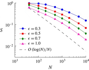
to 2000, which is a substantial amount of sparsification. Let us further show the sparsity index
 $S$
for increasing
 $N$
with different approximation order
 ${\it\epsilon}$
in figure 6. The sparsity index
 $S$
decreases with an increase in
 ${\it\epsilon}$
and the number of vortices. The expected behaviour of the sparsity index,
 $S=O(N\log (N))/(N^{2})=O(\log (N)/N)$
, is observed for larger
 $N$
. The trend deviates from the expected behaviour for lower
 $N$
as the availability of connections for redistribution of the weights of the sparsified connections decreases.
Sparsity patterns of the adjacency matrix for
 $N=500$
(a) and 2000 (b) for approximation order
 ${\it\epsilon}=1$
. The colour in the sparsity patterns of the adjacency matrix denotes the adjacency weights
 $\widetilde{w}_{ij}$
, with the empty white space indicating sparsity.

Variation of the sparsity index
 $S$
for sparsification with an increasing number of point vortices. The reference black line represents
 $\log (N)/N$
.

We observe that the sparsification algorithm provides us with a heavily sparsified model to produce a computationally tractable representation of the vortex-to-vortex interaction. We further note that the sparsification algorithm can be easily parallelized, which is attractive to further reduce the computational waiting time. The bulk motion of clusters of point vortices could be tracked effectively by tracking their individual centroids. The present approach may lead to algorithms similar to fast particle summation methods where near- and far-field effects are taken into consideration (Greengard & Rokhlin Reference Greengard and Rokhlin1987).
4.3. Sparsified-dynamics model
The sparsified vortex interactions can be used for analysing the dynamics of the system of discrete point vortices. Spectral sparsification can be viewed as adjusting the strength of the vortices in the Biot–Savart law through the sparsification factor
 $W$
given by (3.6). We can incorporate the weights of the sparse graph into the Biot–Savart law as
 $$\begin{eqnarray}\frac{\text{d}\boldsymbol{r}_{\boldsymbol{i}}}{\text{d}t}=\mathop{\sum }_{\begin{array}{@{}c@{}}j=1\\ W_{ij}\neq 0\end{array}}^{N}W_{ij}\frac{{\it\kappa}_{j}}{2{\rm\pi}}\frac{\widehat{\boldsymbol{k}}\times (\boldsymbol{r}_{i}-\boldsymbol{r}_{j})}{|\boldsymbol{r}_{i}-\boldsymbol{r}_{j}|^{2}},\end{eqnarray}$$
where
 $W_{ij}$
is the sparsification factor. The above expression significantly reduces the amount of computation compared with the original Biot–Savart law, because the sparsification has made a significant number of elements of
 $W$
be zero, as seen in figures 3 and 5.
To evaluate the effect of sparsification on the dynamics of the point vortices, we consider the same example as presented in § 4.2 with
 $N=100$
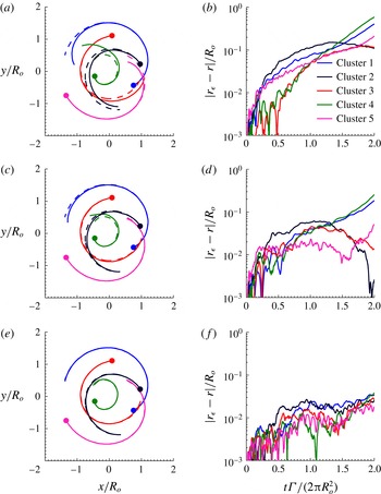
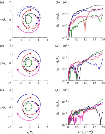
vortices as the initial condition. The objective here is to accurately capture the dynamics of the vortex clusters with the sparsified Biot–Savart law given by (4.4). The bulk motions of the clusters of point vortices are well represented by the centroid of the individual clusters. The original and the sparsified dynamics are given by (4.2) and (4.4) respectively, and are integrated in time with the fourth-order Runge–Kutta method. The results from the sparsified-dynamics model are shown in figures 7 and 8.
Trajectories of the centroids (a,c,e) and error in the positions of the centroids (b,d,f) of the vortex clusters based on the sparse graph (
 ${\it\epsilon}=0.5$
) and the original graph with time for
 $N=100,\bar{{\it\kappa}}=0.1$
. (a,b) Trajectories and error based on sparsification performed only at the initial step. (c,d) Results based on resparsification performed at every (
 $0.1t{\it\Gamma}/2{\rm\pi}R_{o}^{2}$
). (e,f) Results based on resparsification performed at every (
 $0.01t{\it\Gamma}/2{\rm\pi}R_{o}^{2}$
). The full nonlinear solution is shown with dashed lines.

Trajectories of the centroids (a,c,e) and error in the positions of the centroids (b,d,f) of the vortex clusters based on the sparse graph (
 ${\it\epsilon}=1$
) and the original graph with time for
 $N=100,\bar{{\it\kappa}}=0.1$
. (a,b) Trajectories and error based on sparsification performed only at the initial step. (c,d) Results based on resparsification performed at every (
 $0.1t{\it\Gamma}/2{\rm\pi}R_{o}^{2}$
). (e,f) Results based on resparsification performed at every (
 $0.01t{\it\Gamma}/2{\rm\pi}R_{o}^{2}$
). The full nonlinear solution is shown with dashed lines.

For the present analysis, time is non-dimensionalized by considering the cumulative circulation of the vortices of the cluster (
 ${\it\Gamma}$
) and the average radial distance of the centroid of the clusters from the geometric centre of the overall system at the initial time (
 $R_{o}$
). As the advective velocity of an isolated cluster of point vortices of strength
 ${\it\Gamma}$
at
 $R_{o}$
is given by
 $u^{\star }={\it\Gamma}/2{\rm\pi}R_{o}$
, the non-dimensional time can be deduced as
 $tu^{\star }/R_{o}=t{\it\Gamma}/2{\rm\pi}R_{o}^{2}$
. In the present example, each individual cluster has a collection of vortices with their strength having a mean of
 $\bar{{\it\kappa}}=0.1$
(with a normal distribution). Thus, for
 $n$
vortices in a cluster,
 ${\it\Gamma}=n\bar{{\it\kappa}}$
. The error in position of the centroid of the clusters for the sparsified setting with respect to the original setting given by
 $|\boldsymbol{r}_{{\it\epsilon}}-\boldsymbol{r}|$
is non-dimensionalized by the average radial distance of the centroid of the clusters from the geometric centre of the system at the initial time (
 $R_{o}$
).
Let us consider the case where sparsification is performed only once to determine the sparsification factor
 $W_{ij}$
before initiating the time integration. The same sparsification factor is used throughout the time integration. This procedure is inexpensive as sparsification is performed only once a priori. The trace of the positions of the centroid of the individual clusters and their error for approximation orders of
 ${\it\epsilon}=0.5$
and 1 for a single sparsification are shown in figures 7(a,b) and 8(a,b) respectively. Considering the number of connections cut between the vortices for sparse approximations, the trajectories of the centroid of the clusters based on sparse vortex dynamics agree reasonably with those from full dynamics. On comparing the errors, we find that the errors with approximation order of
 ${\it\epsilon}=0.5$
are less than those with
 ${\it\epsilon}=1$
, which is expected. Despite the Biot–Savart law being nonlinear, the present sparsified approach achieves a reasonable agreement with the full nonlinear solution.
If the clusters of vortices are far from each other, the connections cut between their vortices do not cause a large change in the dynamics, while the connections cut between clusters close to each other affect the dynamics considerably. As time progresses, the relative distance between vortices changes, resulting in an increase in error. For
 $t{\it\Gamma}/2{\rm\pi}R_{o}^{2}>1$
, we observe that the error in sparse vortex dynamics increases to
 ${\approx}0.5R_{o}$
. As the adjacency weights
 $w_{ij}$
and the sparsification factor
 $W_{ij}$
are based on the initial position of the vortices, the ratio does not hold over large times. This calls for adjustment of the weights and periodic sparsification to adapt to the dynamically changing position of the vortices.
We thus consider resparsification of the graph representing the system of point vortices periodically at (
 $0.1t{\it\Gamma}/2{\rm\pi}R_{o}^{2}$
) and (
 $0.01t{\it\Gamma}/2{\rm\pi}R_{o}^{2}$
) for both approximation orders. The trace of the centroids and error for approximation orders of
 ${\it\epsilon}=0.5$
and 1 with resparsification are shown in panels (c,d) and (e,f) respectively of figures 7 and 8. We observe that the error decreases significantly with resparsification. The error in position reduces from
 $O(10^{-1})$
to
 $O(10^{-2})$
with resparsification. We notice that the centroid trajectories based on the sparse and original calculations become increasingly similar with resparsification. Resparsification updates the sparsification factor periodically based on the position and strength of the vortices and decreases the error by an order of magnitude. Thus, the nonlinear evolution of discrete vortex dynamics is well predicted by the sparsification techniques.
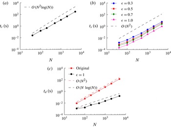
One of the advantages of sparsification is the decreased computational cost due to the increased sparsity of the connections between the vortices. This could potentially lead to the design of faster algorithms based on sparsification strategies. Let us first evaluate the offline cost of computing the effective resistance and random sampling required for spectral sparsification. The time required for computing the effective resistance
 $t_{r}$
and the time required for random sampling
 $t_{s}$
are shown in figure 9(a) and (b) respectively. All computations were performed in MATLAB on an iMac with a 3.4 GHz Intel Core i7 processor. We can observe that for each edge, the computation time of the effective resistance is
 $O(\log (N))$
, hence requiring
 $O(N^{2}\!\log (N))$
for the overall effective resistance computation. The random sampling procedure takes
 $O(N^{2})$
time for all the approximation orders. We compare the computational time
 $t_{d}$
required at each step of numerical integration of the Biot–Savart law for the original and sparse configurations. We can observe from figure 9(c) that the original configuration takes
 $O(N^{2})$
time equivalent to the number of edges in the complete graph, while for the sparse configuration the computation time is reduced to
 $O(N\log (N))$
.
The time required for computation of (a) the effective resistance and (b) the random sampling for different approximation orders for one time sparsification. The dashed lines indicate the expected trends. (c) Time required for numerical integration at each step for the original and sparsified configurations with
 ${\it\epsilon}=1$
.

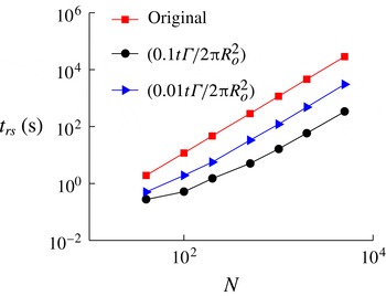
There is always a trade-off amongst the level of sparsification, the error that appears in the dynamics and the associated computational cost. The sparser the network is, the faster the computation can become, but accuracy may be compromised. To increase the computational accuracy, resparsification can be performed, but can introduce an additional computational load. We evaluate the computational cost for numerical integration until a total time of
 $0.1t{\it\Gamma}/2{\rm\pi}R_{o}^{2}$
. The times required for resparsification and numerical integration for the two different resparsification frequencies (performed every
 $0.1t{\it\Gamma}/2{\rm\pi}R_{o}^{2}$
and
 $0.01t{\it\Gamma}/2{\rm\pi}R_{o}^{2}$
) considered in this work for the original and sparse configurations with
 ${\it\epsilon}=1$
are shown in figure 10. It should be noted that for the resparsification performed every
 $0.1t{\it\Gamma}/2{\rm\pi}R_{o}^{2}$
, resparsification is performed once for the total time considered. For the resparsification conducted every
 $0.01t{\it\Gamma}/2{\rm\pi}R_{o}^{2}$
, resparsification is performed ten times. We can see that the time required for resparsification at every
 $0.1t{\it\Gamma}/2{\rm\pi}R_{o}^{2}$
is considerably less compared with the original configuration. With increase in resparsification frequency, although the time required is less compared with the original configuration, there is increased cost associated with resparsification.
The time required for numerical integration for a total time of
 $0.1t{\it\Gamma}/2{\rm\pi}R_{o}^{2}$
with different resparsification frequencies.

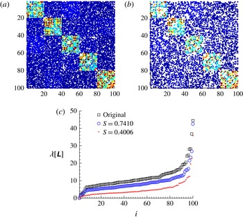
To illustrate that the trajectory prediction using sparsification cannot be performed naively, we compare the results from spectral sparsification with those based on random edge removal (without redistribution of edge weights). We keep the number of cuts identical to that achieved by spectral sparsification for fairness. The sparsity patterns for random cuts with sparsity
 $S=0.7410$
and 0.4006 and the corresponding Laplacian eigenspectra are shown in figure 11. We observe that the spectra from the randomly sparsified graphs grossly underpredict those of the original graph.
Sparsity patterns of the adjacency matrix for
 $N=100$
vortices with random cuts with sparsity (a)
 $S=0.7410$
and (b)
 $S=0.4006$
. The colour in the sparsity patterns of the adjacency matrix indicates the adjacency weights
 $\widetilde{w}_{ij}$
for
 $S=0.7410$
and 0.4006. (c) Eigenvalue spectra of the Laplacian matrices of the randomly sparsified graphs with
 $S=0.7410$
and 0.4006 in comparison with the original graph. The legend for the sparsity patterns is similar to that of sparsity patterns in figure 3.

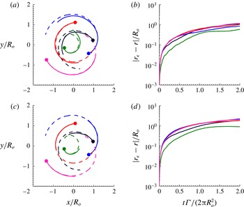
The trace of the positions of the centroid of the individual clusters and their error for random cuts with sparsity
 $S=0.7410$
and 0.4006 for one-time sparsification are shown in figure 12. The random-cut approximation performs poorly compared with spectral sparsification and the dynamics of the centroid of the vortex clusters is not captured. As the connections between the vortices are randomly cut, the centroids of the clusters move slower compared with the original configuration, as expected. This is due to the loss of induced velocity with the absence of weight redistribution from random sparsification. Spectral sparsification, on the other hand, redistributes the weights to prevent the loss of the overall interactions amongst the set of point vortices.
(a,c) Trajectories of the centroids and (b,d) error in the position of the centroids of the vortex clusters based on random cuts with sparsity
 $S=0.7410$
(a,b) and 0.4006 (c,d) for
 $N=100,\bar{{\it\kappa}}=0.1$
.

It is well known that fast multipole methods (Greengard & Rokhlin Reference Greengard and Rokhlin1987) can also reduce the
 $O(N^{2})$
velocity evaluation significantly. The particle–box and box–box schemes reduce the computational complexity from
 $O(N^{2})$
to
 $O(N\log (N))$
and
 $O(N)$
respectively. As seen in this section, spectral sparsification reduces the computational load to
 $O(N\log (N))$
for computing the velocity of the vortices. Fast multipole methods approximate the effect of a cluster of particles at a certain distance by multipole expansions and organizing the particles into a hierarchy of clusters (Cottet & Koumoutsakos Reference Cottet and Koumoutsakos2000). In order to compensate for the sparsified connections in spectral sparsification, the weights are redistributed among the other edge connections to compute the sparsified dynamics. In an analogy to fast multipole methods, the interaction list depends on the connections that have direct impact on the vortices, and the computational accuracy may degrade when the vortices move in space. Similarly to the reconstruction of tree data structures in fast multipole methods, performing resparsification periodically increases the accuracy by re-evaluating the associated weights as the positions of the vortices evolve over time. We note that even with sparsification, invariants of discrete vortices are conserved, as discussed below.
4.4. Conservation properties
For a discrete set of point vortices, the angular impulse and linear impulse are among the conserved quantities. The coordinates of the centre of vorticity obtained from the linear impulse and the length of dispersion about the centre of vorticity obtained from the angular impulse, when the strength of the vortices is of the same sign, remain constant. The centre of vorticity
 $(X,Y)$
and length of dispersion of vorticity
 $D$
are given by
 $$\begin{eqnarray}X=\frac{\displaystyle \mathop{\sum }_{i=1}^{N}{\it\kappa}_{i}x_{i}}{\displaystyle \mathop{\sum }_{j=1}^{N}{\it\kappa}_{j}},\quad Y=\frac{\displaystyle \mathop{\sum }_{i=1}^{N}{\it\kappa}_{i}y_{i}}{\displaystyle \mathop{\sum }_{j=1}^{N}{\it\kappa}_{j}},\end{eqnarray}$$
 $$\begin{eqnarray}D^{2}=\frac{\displaystyle \mathop{\sum }_{i=1}^{N}{\it\kappa}_{i}\{(x_{i}-X)^{2}+(y_{i}-Y)^{2}\}}{\displaystyle \mathop{\sum }_{j=1}^{N}{\it\kappa}_{j}},\end{eqnarray}$$
where
 ${\it\kappa}_{i}$
is the strength of the
 $i$
th vortex and
 $(x,y)$
are the vortex positions (Batchelor Reference Batchelor2000; Newton Reference Newton2001). The circulation for
 $n$
vortices in a cluster is
 ${\it\Gamma}=n\bar{{\it\kappa}}$
. The total circulation of the system of
 $n_{c}=5$
clusters is given by
 ${\it\Gamma}_{t}=\sum _{i=1}^{N}{\it\kappa}_{i}=n_{c}{\it\Gamma}$
. Another conserved quantity is the Hamiltonian. The Hamiltonian is defined as the interaction energy of the system of point vortices and is given by
 $$\begin{eqnarray}H=-\frac{1}{4{\rm\pi}}\mathop{\sum }_{i,j=1,i\neq j}^{N}{\it\kappa}_{i}{\it\kappa}_{j}\log \sqrt{(x_{i}-x_{j})^{2}+(y_{i}-y_{j})^{2}}.\end{eqnarray}$$
We non-dimensionalize the Hamiltonian using the total circulation of
 $n_{c}$
clusters and the average radial distance of the centroid of the clusters at initial time
 $R_{o}$
.
We compare the error in the Hamiltonian
 $(H_{{\it\epsilon}}(r/R_{o})-H(r/R_{o}))/{\it\Gamma}_{t}^{2}$
, the centre of vorticity
 $((X_{{\it\epsilon}}-X)/R_{o},(Y_{{\it\epsilon}}-Y)/R_{o})$
and the square of the length of dispersion of vorticity
 $(D_{{\it\epsilon}}^{2}-D^{2})/R_{o}^{2}$
for approximation orders of
 ${\it\epsilon}=0.5$
and 1 over time in figure 13. The preservation of the centre of vorticity and length of dispersion implies the conservation of linear and angular impulse. Here, the variables with subscript
 ${\it\epsilon}$
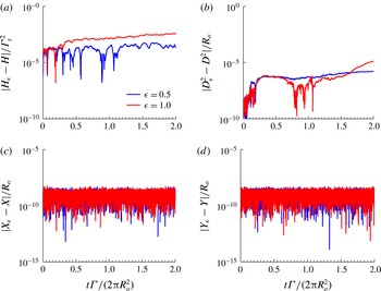
denote those based on a sparsified model. We observe that the error in the Hamiltonian is of
 $O(10^{-4})$
for
 ${\it\epsilon}=0.5$
and
 $O(10^{-3})$
for
 ${\it\epsilon}=1$
. The error in the square of dispersion is of
 $O(10^{-6})$
while the error in the centre of vorticity is of
 $O(10^{-8})$
with sparsification. While not shown, resparsification of these vortices periodically performed at every (
 $0.1t{\it\Gamma}/2{\rm\pi}R_{o}^{2}$
) and (
 $0.01t{\it\Gamma}/2{\rm\pi}R_{o}^{2}$
) maintains similar error levels for the invariants. We also note that the circulation of each vortex has not been altered, which conserves the individual and overall circulation over time.
Error in (a) the Hamiltonian, (b) the square of the length of dispersion, (c) the
 $x$
position of the centre of vorticity and (d) the
 $y$
position of the centre of vorticity based on single sparsification for
 $N=100,\bar{{\it\kappa}}=0.1$
and
 ${\it\epsilon}=\{0.5,1\}$
.

As seen in § 3.1, sparsification by effective resistance is based on the energy-minimization principle. The effective resistance is defined such that the total energy of the system remains constant. This is reflected well in the conservation of the Hamiltonian representing the interaction energy of the discrete point vortices. In addition, sparsification preserves other invariants including the linear and angular impulses of the discrete set of point vortices. We note in passing that even with resparsification, the invariants were observed to be conserved. The conservation of the invariants for the sparse configurations further supports the applicability of sparsification strategies on discrete vortex dynamics.
4.5. Sparsified-dynamics model and reduced-order model
We comment on the similarities and differences between the present sparsified-dynamics model and the reduced-order model. Both models share the general objective of deriving a model that captures the full-order physics in a distilled manner. Reduced-order models achieve such goals by reducing the dimension of the state variable. One such technique is the Galerkin projection of the Navier–Stokes equations using a set of spatial bases (Rowley et al. Reference Rowley, Colonius and Murray2004; Noack et al. Reference Noack, Papas and Monkewitz2005), such as those determined from POD (Berkooz et al. Reference Berkooz, Holmes and Lumley1993; Holmes et al. Reference Holmes, Lumley and Berkooz1996). One can further consider incorporating the effect of input and output dynamics by using balanced truncation or the eigensystem realization algorithm (Rowley Reference Rowley2005; Ma, Ahuja & Rowley Reference Ma, Ahuja and Rowley2009). The resulting reduced-order models are generally described by ordinary differential equations for the temporal coefficients with reduced dimensions.
On the other hand, the present sparsified-dynamics model does not reduce the dimensionality of the state variable. We instead focus on reducing the number of connections used to capture the overall dynamics of the fluid flow. The reduction in the number of connections is performed based on concepts from network analysis and graph theory. Although we cut a large number of the edges in the graph representation of the dynamical interaction, we redistribute the weights associated with the edges to maintain the properties of the graph. This procedure is based upon approximating the spectral properties of the graph and does not require selection of the spatial basis functions, unlike Galerkin-projection-based models. One nice feature of the sparsified-dynamics model is its ability to conserve physical variables such as the Hamiltonian, angular impulse and linear impulse, as discussed above. Hence, the sparsified dynamics is able to predict the full dynamics, as demonstrated by the example with discrete vortices. By highlighting the interactions amongst a set of vortices, we are able to determine which interactions amongst the vortices are important in guiding the overall motion of the vortices.
We believe that the sparsified-dynamics model has promising potential to model various types of fluid flow by considering the modal structures as an abstraction of graph nodes. The application of sparsified-dynamics models towards flow control problems may also become fruitful as the computational time necessary to capture the complex behaviour of the flow is reduced and the interaction of nodes or flow structures is well captured, which has been a feature that is lacking in linear dynamics models and linear stability analysis. We anticipate that the presently proposed model can lead to potential feedback control of fluid flow (Bagheri et al. Reference Bagheri, Hœpffner, Schmid and Henningson2009; Ahuja & Rowley Reference Ahuja and Rowley2010) but with nonlinear interactions emphasized. One of the open questions in extending the sparsified-dynamics model for a wide variety of fluid flow problems is the choice of the variables or modes to be used for graph nodes. This issue is currently being examined and will be reported in upcoming studies.
5. Concluding remarks
Graph representations of a system of discrete point vortices provide us with a framework for identifying important connections amongst vortices. The edge weights of the graph were related to the importance of the ties between the vortices, which were quantified based on the strength of the vortices and the relative distance between them. We sparsified the connections between these vortices based on spectral graph theory not only to cut some of these ties but also to redistribute their weights to preserve the dynamics of the vortices. We have demonstrated that an effective resistance approach to graph sparsification proves extremely useful in constructing sparsified-dynamics models. Moreover, sparsification reduces the number of connections to
 $O(N\log N/{\it\epsilon}^{2})$
based on approximation order
 ${\it\epsilon}$
. We also observed an increase in the effectiveness of sparsification with increasing number of point vortices. In spite of the nonlinear nature of the dynamics of these point vortices, the sparse representations are capable of identifying the core vortex structures as well as tracking the bulk motion of these structures in an effective manner. We have referred to the dynamical model that uses the sparsified vortex network as the sparsified-dynamics model. In addition, the sparsified models preserve the spectral properties of the original set-up. Resparsification is utilized to enhance the prediction of the motion of the vortices over time. We observed that sparsification conserves the invariants of discrete vortex dynamics such as the Hamiltonian, linear and angular impulses, and circulation. The objectives of the sparsified-dynamics model are aligned with those of reduced-order models, but these goals are achieved by sparsifying the connections rather than deriving a model equation with a state variable of reduced dimension. The results of this graph-theoretic approach to discrete vortex dynamics point to promising research into its applicability to a variety of problems in fluid mechanics.
Acknowledgements
We thank Dr M. Jemison and Professor L. Cattafesta for their comments on an earlier version of this paper. This work was supported by the US Air Force Office of Scientific Research (grant FA9550-13-1-0183, Program Manager: Dr D. Smith) and the US Army Research Office (grant W911NF-14-1-0386, Program Manager: Dr S. Stanton). A.G.N. also acknowledges the Aeropropulsion, Mechatronics, and Energy fellowship from the Florida State University.