1. Introduction
Stability of two-dimensional (2D) parallel flows is one of the fundamental problems in fluid dynamics, and bifurcation structures, as well as linear and nonlinear stabilities of many types of planar parallel flows, have been investigated in relation to various fluid phenomena in nature and engineering. In a plane, the 2D parallel flows are dependent only on a single coordinate of an orthogonal coordinate system. Similar problems arise for flows on a non-rotating and rotating sphere. Zonal flows on a sphere, often observed on planets and the sun, are in the azimuthal direction, sometimes making stripe patterns in planetary atmospheres. Note that the rotation has an effect on the 2D incompressible flows on a sphere, while it does not in a planar case.
Baines (Reference Baines1976) studied the inviscid linear stability of typical zonal flows on a sphere, the streamfunction of which is expressed by a single spherical harmonics
 $Y_{l}^{0}$
. He solved the eigenvalue problem numerically by the spectral method. The inflection-point theorem, which gives a sufficient condition for linear stability, says that any zonal flow is linearly stabilized when the rotation rate is large enough (see Kuo Reference Kuo1949). Therefore the inviscid zonal flow has the critical rotation rate at which it is marginally stable. He obtained the critical rotation rate numerically, and found that it is only slightly different from the estimates obtained from the inflection-point theorem. Recently, Sasaki, Takehiro & Yamada (Reference Sasaki, Takehiro and Yamada2012), however, re-studied the linear stability of the inviscid zonal flows in the same way as Baines (Reference Baines1976) but with a higher truncation wavenumber. They found that the numerical calculation is still problematic because of emergence of the critical layer, and obtained accurate values of the critical rotation rates with special attention to the critical layers. On the other hand, in the viscous case, Sasaki, Takehiro & Yamada (Reference Sasaki, Takehiro and Yamada2013) studied the linear stability of the same type of zonal flow. They found that as the rotation rate increases, the critical Reynolds number, where zonal flow loses stability, increases rapidly, and zonal flow is linearly stable at Reynolds numbers less than
 $10^{6}$
when the rotation rate is large enough. This stabilization by rotation appears to be consistent with the inviscid case described above.
In this paper we first study the nonlinear regime of the stability of viscous zonal flows on a rotating sphere, i.e. the bifurcation structure of zonal flows, with the Reynolds number and the rotation rate being the bifurcation parameters. We consider 2D incompressible viscous zonal flows driven by a forcing expressed by a single spherical harmonics
 $Y_{l}^{0}$
. In a limited range of the rotation rate including the non-rotating case, we find that zonal flows are unstable when the Reynolds number is large enough. In order to find how the solution behaves in the unstable region, we carry out numerical time integration at high Reynolds numbers in the non-rotating case, and study the possibility of describing the chaotic solution with a linear combination of unstable steady and travelling solutions.
We should remark that our problem setting is similar to the Kolmogorov problem (Obukhov Reference Obukhov1983). The Kolmogorov problem was first proposed by Kolmogorov in his seminar in the 1960s to study mathematical structures of solutions of the Navier–Stokes equations. The problem deals with a viscous incompressible 2D fluid in a double-periodic domain, a flat torus, with sine-type unidirectional external forcing, and gives a typical and fundamental example of transitions from laminar flow to turbulence. Iudovisch (Reference Iudovisch1965) proved that two-jet parallel flow is globally stable for arbitrary Reynolds number, and Meshalkin & Sinai (Reference Meshalkin and Sinai1962) proved that the critical modes of the parallel flow are steady (not Hopf), while Iudovisch (Reference Iudovisch1965) proved the existence of the bifurcation solution arising at the critical stability. The bifurcation diagram of steady solutions arising from the two-jet parallel flow was studied by Okamoto & Shōji (Reference Okamoto and Shōji1993) for several aspect ratios of the flat torus. They found various types of bifurcation, including saddle-node bifurcation, Hopf bifurcation and secondary bifurcation. The inviscid limit of bifurcating steady solutions was studied by Kim & Okamoto (Reference Kim and Okamoto2010). They found that the flow field of nonlinear solutions becomes dominated by a pair of negative and positive vortices at high Reynolds numbers regardless of the forcing wavenumber, although those patterns are constructed by multiple vortices at low Reynolds numbers. They called this solution a unimodal solution, and suggested that at high Reynolds numbers there is at least one unimodal solution, independent of the number of jets of the original parallel flow. Note that the Kolmogorov problem has been studied from several perspectives including transition to chaos (Platt, Sirovich & Fitzmaurice Reference Platt, Sirovich and Fitzmaurice1991), the orbital instability of chaotic flow (Inubushi et al. Reference Inubushi, Kobayashi, Takehiro and Yamada2012) and the extraction of invariant sets from chaotic attractors (Lucas & Kerswell Reference Lucas and Kerswell2015). We will compare our results on a sphere with those of Kolmogorov flows in a planar domain. We note that a sphere (genus 0) is topologically simpler than a torus (genus 1), while a sphere has a non-zero curvature and is more complicated in the sense of differential geometry than the flat torus.
In the following, we discuss the bifurcation structure of 2D incompressible viscous zonal flows on a non-rotating/rotating sphere under zonal forcing. In § 2 we describe the governing equation, and in § 3 we prove the global stability of two-jet zonal flow. In § 4 we show bifurcation diagrams of the steady solutions arising from three-jet zonal flow, and in § 5 we discuss unsteady solutions at high Reynolds numbers. Section 6 is devoted to the discussions and conclusions.
2. Governing equations
We consider 2D incompressible viscous flow on a rotating sphere governed by the non-dimensional vorticity equation
 $$\begin{eqnarray}\frac{\partial {\rm\Delta}{\it\psi}}{\partial t}+J({\it\psi},{\rm\Delta}{\it\psi})+2{\it\Omega}\frac{\partial {\it\psi}}{\partial {\it\lambda}}=\frac{1}{\mathit{Re}}\{({\rm\Delta}+2){\rm\Delta}{\it\psi}+(l(l+1)-2)Y_{l}^{0}({\it\mu})\}.\end{eqnarray}$$
Here
 $t$
represents the time, while
 ${\it\lambda}$
and
 ${\it\mu}$
denote the longitude and the sine latitude,
 ${\it\mu}=\sin {\it\phi}$
, where
 ${\it\phi}$
is the latitude. The streamfunction is denoted by
 ${\it\psi}$
, and the vorticity is given by
 ${\rm\Delta}{\it\psi}={\it\zeta}$
, where
 ${\rm\Delta}$
is the horizontal Laplacian on the unit sphere. The longitudinal and latitudinal components of velocity
 $(u_{{\it\lambda}},u_{{\it\mu}})$
are expressed by
 $u_{{\it\lambda}}=-(1-{\it\mu}^{2})^{1/2}(\partial {\it\psi}/\partial {\it\mu})$
and
 $u_{{\it\mu}}=(1-{\it\mu}^{2})^{-1/2}(\partial {\it\psi}/\partial {\it\lambda})$
, respectively. The parameter
 $\mathit{Re}$
is the Reynolds number,
 ${\it\Omega}$
is the non-dimensional rotation rate of the sphere and
 $J(A,B)$
is the Jacobian
 $(\partial A/\partial {\it\lambda})(\partial B/\partial {\it\mu})-(\partial A/\partial {\it\mu})(\partial B/\partial {\it\lambda})$
. The flow is driven by the vorticity forcing,
 $(l(l+1)-2)Y_{l}^{0}({\it\mu})/\mathit{Re}$
, where
 $Y_{l}^{m}({\it\lambda},{\it\mu})$
is a
 $4{\rm\pi}$
-normalized spherical harmonics with the total wavenumber
 $l$
and the longitudinal wavenumber
 $m$
. In addition, the term of
 $2{\rm\Delta}{\it\psi}/\mathit{Re}$
in the viscosity term is necessary for the conservation of the total angular momentum of the system (see Silberman Reference Silberman1953).
The vorticity equation (2.1) has a steady
 $l$
-jet zonal flow solution for arbitrary Reynolds number and the rotation rate, expressed by
 $$\begin{eqnarray}{\it\psi}_{0}({\it\mu})=-\frac{1}{l(l+1)}Y_{l}^{0}({\it\mu}),\quad {\it\zeta}_{0}({\it\mu})=Y_{l}^{0}({\it\mu}).\end{eqnarray}$$
Note that this solution is independent of the Reynolds number. Here, the number of jets is defined as the number of extreme points of the longitudinal velocity, which is equivalent to the number of the nodes of the latitudinal distribution of the streamfunction. The steady
 $l$
-jet solution (2.2) is the only steady solution independent of
 ${\it\lambda}$
. Hereafter we call this solution the trivial solution.
We should note a similar problem named after Kolmogorov, who proposed to study solutions of 2D incompressible viscous flow on a doubly periodic domain (a flat torus). His school studied the problem under the vorticity forcing of
 $n^{2}\,\text{cos}\,ny/\mathit{Re}$
, yielding a
 $2n$
-jet parallel flow with the streamfunction being
 $-\!\cos (ny)/n^{2}$
. In the Kolmogorov problem, the flow becomes unstable as
 $\mathit{Re}$
increases, and goes through several bifurcations to turbulent states. The sinusoidal forcing given by the single sine function, which is the eigenfunction of the Laplacian on the flat torus, makes the nonlinear terms vanish for the
 $2n$
-jet parallel flows. In our problem on a sphere, the forcing term is a single spherical harmonic function
 $Y_{l}^{0}({\it\mu})$
, which is also an eigenfunction of the Laplacian on a sphere and makes the nonlinear terms vanish for the trivial steady
 $l$
-jet solution. Thus our problem setting may be regarded as a spherical version of the Kolmogorov problem, and, from this point of view, it should be noted that the topology of the flow domain is simpler in our case (sphere of genus 0) than in the Kolmogorov problem (torus of genus 1).
3. Global stability of two-jet zonal flow
In the case of
 $l=1$
, the trivial solution is one-jet zonal flow. This is a special case in which the energy injection vanishes. Since the coefficient of
 $Y_{1}^{0}$
in the spherical harmonic expansion of the streamfunction is proportional to the total angular momentum along the rotation axis of the sphere, the amplitude of the
 $Y_{1}^{0}$
component remains constant over time. On the other hand, the
 $Y_{1}^{-1}$
and
 $Y_{1}^{1}$
components keep oscillations with constant (complex) amplitudes. Therefore, under the viscous effect the disturbance to one-jet zonal flow decays to zero except for its
 $l=1$
components, which stay on the constant amplitudes. In this sense, one-jet zonal flow is stable for any Reynolds number and any rotation rate. This conclusion is also obtained from another point of view when one-jet zonal flow corresponds to the rest state in an appropriate rotating frame of reference.
Next we consider the case of
 $l=2$
, where the energy injection does not vanish, but we can prove the global stability of the trivial zonal flow for arbitrary Reynolds number and the rotation rate.
Substituting
 ${\it\psi}({\it\lambda},{\it\mu},t)=AY_{2}^{0}({\it\mu})+\tilde{{\it\psi}}({\it\lambda},{\it\mu},t)$
 $(A=-1/6)$
into (2.1) and omitting the tilde, we obtain
 $$\begin{eqnarray}\partial _{t}{\rm\Delta}{\it\psi}+J(AY_{2}^{0},({\rm\Delta}+6){\it\psi})+2{\it\Omega}\partial _{{\it\lambda}}{\it\psi}+J({\it\psi},{\rm\Delta}{\it\psi})-\frac{1}{\mathit{Re}}({\rm\Delta}+2){\rm\Delta}{\it\psi}=0.\end{eqnarray}$$
The inner products of
 ${\it\psi}$
and
 ${\rm\Delta}{\it\psi}$
yields
 $$\begin{eqnarray}\displaystyle & \displaystyle \frac{1}{2}\partial _{t}\Vert \boldsymbol{{\rm\nabla}}{\it\psi}\Vert ^{2}+\frac{1}{\mathit{Re}}(\Vert {\rm\Delta}{\it\psi}\Vert ^{2}-2\Vert \boldsymbol{{\rm\nabla}}{\it\psi}\Vert ^{2})+\int \,\text{d}S\,{\it\psi}A(\partial _{{\it\mu}}Y_{2}^{0})({\rm\Delta}\partial _{{\it\lambda}}{\it\psi})=0, & \displaystyle\end{eqnarray}$$
 $$\begin{eqnarray}\displaystyle & \displaystyle \frac{1}{2}\partial _{t}\Vert {\rm\Delta}{\it\psi}\Vert ^{2}+\frac{1}{\mathit{Re}}(\Vert \boldsymbol{{\rm\nabla}}{\rm\Delta}{\it\psi}\Vert ^{2}-2\Vert {\rm\Delta}{\it\psi}\Vert ^{2})+6\int \,\text{d}S\,{\it\psi}A(\partial _{{\it\mu}}Y_{2}^{0})({\rm\Delta}\partial _{{\it\lambda}}{\it\psi})=0. & \displaystyle\end{eqnarray}$$
 $\Vert \cdot \Vert$
is defined as
 $$\begin{eqnarray}\Vert f({\it\lambda},{\it\mu})\Vert ^{2}:=\int \,\text{d}S\,f^{2}({\it\lambda},{\it\mu})=\int _{-1}^{1}\,\text{d}{\it\mu}\int _{0}^{2{\rm\pi}}\,\text{d}{\it\lambda}\,f^{2}({\it\lambda},{\it\mu}),\end{eqnarray}$$
and we have used the periodic boundary condition with respect to
 ${\it\lambda}$
, and
 $$\begin{eqnarray}\int \,\text{d}SJ(f,g)h=\int \,\text{d}S\,fJ(g,h).\end{eqnarray}$$
Equations (3.2) and (3.3) yield
 $$\begin{eqnarray}\displaystyle & & \displaystyle \partial _{t}\left\{\frac{1}{2}\left(\frac{1}{6}\Vert {\rm\Delta}{\it\psi}\Vert ^{2}-\Vert \boldsymbol{{\rm\nabla}}{\it\psi}\Vert ^{2}\right)\right\}+\frac{1}{\mathit{Re}}\left\{\frac{1}{6}\Vert \boldsymbol{{\rm\nabla}}{\rm\Delta}{\it\psi}\Vert ^{2}-\Vert {\rm\Delta}{\it\psi}\Vert ^{2}\right\}\nonumber\\ \displaystyle & & \displaystyle \quad -\,\frac{2}{\mathit{Re}}\left\{\frac{1}{6}\Vert {\rm\Delta}{\it\psi}\Vert ^{2}-\Vert \boldsymbol{{\rm\nabla}}{\it\psi}\Vert ^{2}\right\}=0.\end{eqnarray}$$
We split the disturbance
 ${\it\psi}$
into
 ${\it\psi}_{2}$
and
 ${\it\psi}_{rest}$
defined as
 $$\begin{eqnarray}{\it\psi}_{2}=\mathop{\sum }_{m}{\it\psi}_{2}^{m}(t)Y_{2}^{m}({\it\lambda},{\it\mu}),\quad {\it\psi}_{rest}=\mathop{\sum }_{n\geqslant 3,m}{\it\psi}_{n}^{m}(t)Y_{n}^{m}({\it\lambda},{\it\mu}).\end{eqnarray}$$
Substituting
 ${\it\psi}({\it\lambda},{\it\mu},t)={\it\psi}_{2}+{\it\psi}_{rest}$
into (3.6), we obtain
 $$\begin{eqnarray}\displaystyle & & \displaystyle \partial _{t}\left\{\frac{1}{2}\left(\frac{1}{6}\Vert {\rm\Delta}{\it\psi}_{rest}\Vert ^{2}-\Vert \boldsymbol{{\rm\nabla}}{\it\psi}_{rest}\Vert ^{2}\right)\right\}\nonumber\\ \displaystyle & & \displaystyle \qquad +\,\frac{1}{\mathit{Re}}\left\{\frac{1}{6}\Vert \boldsymbol{{\rm\nabla}}{\rm\Delta}{\it\psi}_{rest}\Vert ^{2}-\Vert {\rm\Delta}{\it\psi}_{rest}\Vert ^{2}\right\}-\frac{2}{\mathit{Re}}\left\{\frac{1}{6}\Vert {\rm\Delta}{\it\psi}_{rest}\Vert ^{2}-\Vert \boldsymbol{{\rm\nabla}}{\it\psi}_{rest}\Vert ^{2}\right\}=0.\nonumber\\ \displaystyle & & \displaystyle\end{eqnarray}$$
The second term of (3.8) is evaluated as
 $$\begin{eqnarray}\displaystyle \frac{1}{6}\Vert \boldsymbol{{\rm\nabla}}{\rm\Delta}{\it\psi}_{rest}\Vert ^{2}-\Vert {\rm\Delta}{\it\psi}_{rest}\Vert ^{2} & {\geqslant} & \displaystyle 12\mathop{\sum }_{n\geqslant 3,m}n(n+1)\left(\frac{n(n+1)}{6}-1\right)|{\it\psi}_{n}^{m}|^{2}\nonumber\\ \displaystyle & = & \displaystyle 12\left(\frac{1}{6}\Vert {\rm\Delta}{\it\psi}_{rest}\Vert ^{2}-\Vert \boldsymbol{{\rm\nabla}}{\it\psi}_{rest}\Vert ^{2}\right).\end{eqnarray}$$
Thus we obtain
 $$\begin{eqnarray}\frac{1}{6}\Vert {\rm\Delta}{\it\psi}_{rest}\Vert ^{2}-\Vert \boldsymbol{{\rm\nabla}}{\it\psi}_{rest}\Vert ^{2}\leqslant C_{0}\exp \left(-\frac{20}{\mathit{Re}}t\right),\end{eqnarray}$$
where
 $C_{0}$
is a constant depending on the initial condition of disturbance. Hereafter we denote other constants similarly, i.e.
 $C_{i}\;(i=1,\dots ,5)$
. Using the obvious inequality
 $$\begin{eqnarray}\Vert {\rm\Delta}{\it\psi}_{rest}\Vert ^{2}\geqslant 12\Vert \boldsymbol{{\rm\nabla}}{\it\psi}_{rest}\Vert ^{2}\geqslant 12^{2}\Vert {\it\psi}_{rest}\Vert ,\end{eqnarray}$$
we have
 $$\begin{eqnarray}\Vert {\it\psi}_{rest}\Vert \leqslant C_{1}\exp \left(-\frac{10}{\mathit{Re}}t\right).\end{eqnarray}$$
Next, taking the inner product of
 ${\it\psi}_{2}$
and (3.1), we obtain
 $$\begin{eqnarray}\partial _{t}\Vert {\it\psi}_{2}\Vert +\frac{4}{\mathit{Re}}\Vert {\it\psi}_{2}\Vert =\frac{1}{6}\left\{\int \!\frac{{\it\psi}_{2}}{\Vert {\it\psi}_{2}\Vert }J(AY_{2}^{0},({\rm\Delta}+6){\it\psi}_{rest})+\int \!\frac{{\it\psi}_{2}}{\Vert {\it\psi}_{2}\Vert }J({\it\psi}_{rest},{\rm\Delta}{\it\psi}_{rest})\right\}.\end{eqnarray}$$
The first term on the right-hand side can be evaluated as
 $$\begin{eqnarray}\displaystyle \left|\int \!\frac{{\it\psi}_{2}}{\Vert {\it\psi}_{2}\Vert }J(AY_{2}^{0},({\rm\Delta}+6){\it\psi}_{rest})\right| & {\leqslant} & \displaystyle \left|\int \!\frac{1}{\Vert {\it\psi}_{2}\Vert }J({\it\psi}_{2},AY_{2}^{0}){\rm\Delta}{\it\psi}_{rest}\right|\nonumber\\ \displaystyle & & \displaystyle +\,6\left|\int \!\frac{1}{\Vert {\it\psi}_{2}\Vert }{\it\psi}_{2}J(AY_{2}^{0},{\it\psi}_{rest})\right|\nonumber\\ \displaystyle & {\leqslant} & \displaystyle \frac{1}{\Vert {\it\psi}_{2}\Vert }\Vert \boldsymbol{{\rm\nabla}}{\it\psi}_{2}\times \boldsymbol{{\rm\nabla}}AY_{2}^{0}\Vert \,\Vert {\rm\Delta}{\it\psi}_{rest}\Vert \nonumber\\ \displaystyle & & \displaystyle +\,6\frac{1}{\Vert {\it\psi}_{2}\Vert }\Vert {\it\psi}_{2}\Vert \,\Vert \boldsymbol{{\rm\nabla}}AY_{2}^{0}\times \boldsymbol{{\rm\nabla}}{\it\psi}_{rest}\Vert \nonumber\\ \displaystyle & {\leqslant} & \displaystyle \Vert A\boldsymbol{{\rm\nabla}}Y_{2}^{0}\Vert (\sqrt{6}\Vert {\rm\Delta}{\it\psi}_{rest}\Vert +6\Vert \boldsymbol{{\rm\nabla}}{\it\psi}_{rest}\Vert )\nonumber\\ \displaystyle & {\leqslant} & \displaystyle C_{2}\exp \left(-\frac{10}{\mathit{Re}}t\right),\end{eqnarray}$$
and the second term on the right-hand side becomes
 $$\begin{eqnarray}\displaystyle \left|\int \frac{{\it\psi}_{2}}{\Vert {\it\psi}_{2}\Vert }J({\it\psi}_{rest},{\rm\Delta}{\it\psi}_{rest})\right| & {\leqslant} & \displaystyle \frac{1}{\Vert {\it\psi}_{2}\Vert }\Vert \boldsymbol{{\rm\nabla}}{\it\psi}_{2}\times \boldsymbol{{\rm\nabla}}{\it\psi}_{rest}\Vert \,\Vert {\rm\Delta}{\it\psi}_{rest}\Vert \nonumber\\ \displaystyle & {\leqslant} & \displaystyle \sqrt{6}\Vert \boldsymbol{{\rm\nabla}}{\it\psi}_{rest}\Vert \,\Vert {\rm\Delta}{\it\psi}_{rest}\Vert \nonumber\\ \displaystyle & {\leqslant} & \displaystyle C_{3}\exp \left(-\frac{20}{\mathit{Re}}t\right),\end{eqnarray}$$
where we have used the Cauchy–Schwarz inequality and (3.12). Therefore we have
 $$\begin{eqnarray}\partial _{t}\Vert {\it\psi}_{2}\Vert +\frac{4}{\mathit{Re}}\Vert {\it\psi}_{2}\Vert \leqslant C_{4}\exp \left(-\frac{10}{\mathit{Re}}t\right),\end{eqnarray}$$
which with (3.12) leads to an upper bound on the disturbance
 ${\it\psi}={\it\psi}_{2}+{\it\psi}_{rest}$
,
 $$\begin{eqnarray}\Vert {\it\psi}(t)\Vert \leqslant C_{5}\exp \left(-\frac{4}{\mathit{Re}}t\right)\rightarrow 0\quad (t\rightarrow +\infty ).\end{eqnarray}$$
Thus we conclude that two-jet zonal flow is globally asymptotically stable for arbitrary Reynolds number and rotation rate. This conclusion is obtained under the assumption of a steady zonal forcing of
 $Y_{2}^{0}$
, and we can make no reliable statement for the flow pattern when another type of forcing is employed. However, Obuse, Takehiro & Yamada (Reference Obuse, Takehiro and Yamada2010) showed numerically that a two-jet solution is one of the final states when a random high-wavenumber forcing is employed, suggesting global stability of two-jet zonal flow in a more general configuration.
4. Bifurcation structure of steady solutions arising from three-jet zonal flow
4.1. Numerical method
In the case of
 $l=3$
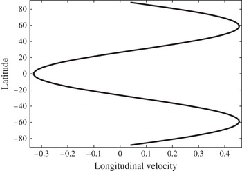
a trivial zonal flow (three-jet flow, figure 1) has been found to be unstable when the Reynolds number is sufficiently large (Sasaki et al.
Reference Sasaki, Takehiro and Yamada2013). A three-jet zonal flow becomes Hopf unstable at a critical Reynolds number which depends on the rotation rate
 ${\it\Omega}$
, for
 ${\it\Omega}_{c}^{-}(=-5.727)<{\it\Omega}<{\it\Omega}_{c}^{+}(=2.171)$
. Outside this interval of
 ${\it\Omega}$
, three-jet flow is linearly stable for any Reynolds number. In this section we study nonlinear solutions of the vorticity equation, focusing on steady and travelling-wave solutions for
 $({\it\Omega}_{c}^{-}<)-5.7\leqslant {\it\Omega}\leqslant 2.1({<}{\it\Omega}_{c}^{+})$
and
 $1\leqslant \mathit{Re}\leqslant 10^{4}$
.
The longitudinal velocity of the three-jet trivial solution. The horizontal and vertical axes indicate longitudinal velocity and latitude.

In order to obtain the numerical solutions, a spectral method with a spherical harmonics expansion is employed, where the streamfunction
 ${\it\psi}$
is expressed as
 $$\begin{eqnarray}{\it\psi}({\it\lambda},{\it\mu})=\mathop{\sum }_{n=1}^{T_{N}}\mathop{\sum }_{m=-n}^{n}{\it\psi}_{n}^{m}Y_{n}^{m}({\it\lambda},{\it\mu}),\end{eqnarray}$$
where
 ${\it\psi}_{n}^{m}$
is the expansion coefficient and
 $T_{N}$
is the truncation wavenumber. We adopt the transform method to evaluate the nonlinear term in (2.1), eliminating the aliasing error. We have checked the accuracy by changing
 $T_{N}$
up to 170. The Newton method is adopted to obtain the steady and travelling solutions.
4.2. Bifurcation diagram in the non-rotating case
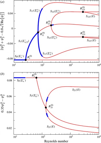
We show the bifurcation diagram of the steady and travelling wave solutions for
 ${\it\Omega}=0$
,
 $1\leqslant \mathit{Re}\leqslant 10^{4}$
in figure 2. Hereafter we denote the solutions in a systematic manner. For example, the solution
 $S_{12}^{(0)}$
means that it originates from the second bifurcation point on the solution branch
 $S_{1}^{(0)}$
, where the superscript
 $(0)$
shows the rotation rate of the sphere. The bifurcating points are expressed similarly:
 $B_{12}^{(0)}$
is the second bifurcation point on the solution branch
 $S_{1}^{(0)}$
.
Bifurcation diagrams in the non-rotating case: (a) bifurcating branches from
 $B_{1}^{(0)}$
, and (b) bifurcating branches from
 $B_{2}^{(0)}$
. The notation of solutions and symmetries is described in the text. The blue (thick) and red (thin) lines denote linearly stable and unstable branches, respectively. The Reynolds numbers at
 $B_{1}^{(0)},B_{11}^{(0)},B_{12}^{(0)},B_{121}^{(0)},B_{2}^{(0)}$
and
 $B_{21}^{(0)}$
, are 26.12, 70.66, 203.8, 2687, 62.51 and 136.2, respectively. Meanwhile,
 $S_{1}^{(0)}$
and
 $S_{11}^{(0)}$
become Hopf unstable at
 $\mathit{Re}=249.4$
and 103.2, respectively. At these critical Reynolds numbers no steady or steady-travelling solution arises. In addition,
 $S_{21}^{(0)}$
is Hopf unstable except for the interval
 $143.5\leqslant \mathit{Re}\leqslant 161.9$
.

As for the symmetry of the streamfunctions, we focus on the following three types of operations. The first one is the longitudinal translation by
 ${\it\alpha}(\neq 0)$
,
 $$\begin{eqnarray}{\it\sigma}_{{\it\alpha}}:{\it\psi}({\it\lambda},{\it\mu})\rightarrow {\it\psi}({\it\lambda}-{\it\alpha},{\it\mu}).\end{eqnarray}$$
The second one is the sign inversion,
 $$\begin{eqnarray}{\it\sigma}_{-}:{\it\psi}({\it\lambda},{\it\mu})\rightarrow -{\it\psi}({\it\lambda},{\it\mu}).\end{eqnarray}$$
The last one is the reflection with respect to the equator,
 $$\begin{eqnarray}{\it\sigma}_{r}:{\it\psi}({\it\lambda},{\it\mu})\rightarrow {\it\psi}({\it\lambda},-{\it\mu}).\end{eqnarray}$$
We let
 ${\it\Sigma}_{{\it\alpha}}$
denote the symmetry group generated by
 ${\it\sigma}_{{\it\alpha}}$
. Similarly,
 ${\it\Sigma}_{{\it\alpha}}^{+}$
denotes the group generated by
 $({\it\sigma}_{{\it\alpha}}{\it\sigma}_{r})$
, and
 ${\it\Sigma}_{{\it\alpha}}^{-}$
denotes the group generated by
 $({\it\sigma}_{{\it\alpha}}{\it\sigma}_{r}{\it\sigma}_{-})$
. We use the symbol
 ${\it\Sigma}_{\ast }$
to express the group consisting of arbitrary longitudinal translations. We let
 $E$
denote the trivial group consisting only of the identity transformation.
The streamfunction of the trivial zonal solution
 $S_{0}$
has symmetry group
 ${\it\Sigma}_{\ast }^{-}$
and becomes Hopf unstable at
 $B_{1}^{(0)}(\mathit{Re}=26.13)$
. Then the travelling-wave solution
 $S_{1}^{(0)}$
bifurcates with symmetry group
 ${\it\Sigma}_{{\rm\pi}/2}^{-}$
, losing the invariance to an arbitrary longitudinal translation. The
 $S_{1}^{(0)}$
again becomes unstable at
 $B_{11}^{(0)}$
with a new branch of
 $S_{11}^{(0)}$
which has symmetry group
 ${\it\Sigma}_{{\rm\pi}}$
, losing equatorial anti-symmetry. Note that the upper and lower branches of
 $S_{11}^{(0)}$
are related to each other by equatorial mirror symmetry. In the parameter range of our calculation, as depicted in figure 2, we found two Hopf bifurcation points and five pitchfork bifurcation points, and all the steady and steady-travelling solutions are found to be Hopf unstable in the range
 $249.4\leqslant \mathit{Re}\leqslant 10^{4}$
.
4.3. Bifurcation diagrams in the rotating case
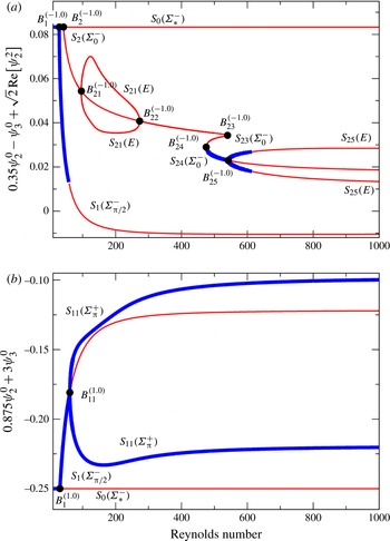
The bifurcation structure of steady and steady-travelling wave solutions is varied by the rotation of the sphere. Numerical results at
 ${\it\Omega}=\pm 1.0$
are shown in figure 3.
Bifurcation diagrams in the rotating cases: (a)
 ${\it\Omega}=-1.0$
and (b)
 ${\it\Omega}=1.0$
. In (a) the Reynolds numbers at bifurcating points are
 $\mathit{Re}=28.94(B_{1}^{(-1.0)}),41.57(B_{2}^{(-1.0)}),95.72(B_{21}^{(-1.0)}),274.5(B_{22}^{(-1.0)}),540.05(B_{23}^{(-1.0)}),475.33(B_{24}^{(-1.0)}),$
and
 $542.4(B_{25}^{(-1.0)})$
. The solutions
 $S_{1}^{(-1.0)}$
and
 $S_{25}^{(-1.0)}$
become Hopf unstable at
 $\mathit{Re}=58.29$
and 614.4, respectively. In (b) the Reynolds numbers at bifurcating points are
 $31.00(B_{1}^{(1.0)})$
and
 $61.11(B_{11}^{(1.0)})$
.

In the case of
 ${\it\Omega}=-1.0$
, the trivial zonal solution
 $S_{0}$
becomes Hopf unstable at
 $B_{1}^{(-1.0)}$
, where a new solution
 $S_{1}^{(-1.0)}$
arises which again becomes unstable at
 $\mathit{Re}=58.29$
.
 $S_{0}$
has the second bifurcation point
 $B_{2}^{(-1.0)}$
, where an unstable branch arises and again has the bifurcation point
 $B_{21}^{(-1.0)}$
. The upper and the lower branches of
 $S_{21}^{(-1.0)}$
contact each other at the next bifurcation point
 $B_{22}^{(-1.0)}$
on the branch of
 $S_{2}^{(-1.0)}$
. Thus these upper and the lower branches make a closed loop connecting
 $B_{21}^{(-1.0)}$
and
 $B_{22}^{(-1.0)}$
. Tracking the
 $S_{2}$
branch further, we find two saddle-node bifurcation points
 $B_{23}^{(-1.0)}$
and
 $B_{24}^{(-1.0)}$
.
In the case of
 ${\it\Omega}=1.0$
, the bifurcation diagram is found to be quite simple compared to that of
 ${\it\Omega}=-1.0$
. After a Hopf bifurcation at
 $B_{1}^{(1.0)}$
, we find only one secondary pitchfork bifurcation point
 $B_{11}^{(1.0)}$
on the branch of
 $S_{1}^{(1.0)}$
. The solution
 $S_{11}^{(1.0)}$
is found to be stable in the range of our calculation,
 $61.11\leqslant \mathit{Re}\leqslant 10^{4}$
. These results show that the bifurcation structure changes drastically by the effect of the rotation.
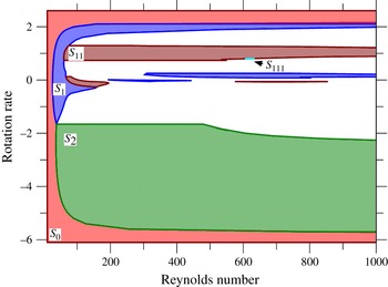
Figure 4 shows solutions which are linearly stable and realizable when the Reynolds number is gradually increased, i.e. the solutions in this figure are connected to the trivial zonal flow
 $S_{0}$
through the stable branches of solutions. There are other branches of stable solutions, but there is no stable branch connecting them to
 $S_{0}$
. It should be remarked that we can find a linearly stable solution in most of the region except for small values of
 $|{\it\Omega}|$
, even for large Reynolds numbers. Note also that the diagram is asymmetric with respect to
 ${\it\Omega}=0$
. The trivial zonal solution
 $S_{0}$
remains linearly stable even for large Reynolds number when
 $|{\it\Omega}|$
is sufficiently large, as already pointed out in the study of linear stability of
 $S_{0}$
by Sasaki et al. (Reference Sasaki, Takehiro and Yamada2012).
Linearly stable solutions which are connected to the trivial zonal flow
 $S_{0}$
through the stable branches of solutions. The red, blue, maroon, light blue and green regions represent the stable regions of the solutions
 $S_{0},S_{1},S_{11},S_{111}$
and
 $S_{2}$
, respectively.

4.4. Flow fields of the nonlinear solutions at large Reynolds numbers
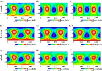
Figure 5 shows the streamfunction of
 $S_{1}$
for
 ${\it\Omega}=0.0,1.0$
and
 $-1.0$
. The solution
 $S_{1}$
has symmetry group
 ${\it\Sigma}_{{\rm\pi}/2}^{-}$
. In the non-rotating case, we find that, as the Reynolds number increases, the vorticity pattern, which is not symmetric with respect to the equator (figure 5
a), approaches a symmetric pattern (figure 5
b), and the streamfunction of
 $S_{1}$
at
 $\mathit{Re}=10^{6}$
almost recovers the symmetry
 ${\it\Sigma}^{+}$
(figure 5
c).
Streamfunctions of
 $S_{1}$
: (a)
 ${\it\Omega}=0,\mathit{Re}=10^{2}$
, (b)
 ${\it\Omega}=0,\mathit{Re}=10^{3}$
, (c)
 ${\it\Omega}=0,\mathit{Re}=10^{6}$
, (d)
 ${\it\Omega}=1.0,\mathit{Re}=10^{2}$
, (e)
 ${\it\Omega}=1.0,\mathit{Re}=10^{3}$
, ( f)
 ${\it\Omega}=1.0,\mathit{Re}=10^{6}$
, (g)
 ${\it\Omega}=-1.0,\mathit{Re}=10^{2}$
, (h)
 ${\it\Omega}=-1.0,\mathit{Re}=10^{3}$
, and (i)
 ${\it\Omega}=-1.0,\mathit{Re}=10^{6}$
, respectively.

In the cases of
 ${\it\Omega}=\pm 1.0$
, we find that the streamfunction of
 $S_{1}$
remains non-symmetric with respect to the equator and does not recover
 ${\it\Sigma}^{+}$
even at high Reynolds numbers. The flow field seems to change little as
 $\mathit{Re}\;({\gtrsim}10^{3})$
increases.
5. Properties of unsteady solutions at high Reynolds numbers
In this section we study numerically the unsteady solutions at high Reynolds numbers. We take as the initial condition a steady or steady-travelling solution superimposed by a disturbance which has the form
 $$\begin{eqnarray}{\it\delta}{\it\psi}({\it\lambda},{\it\mu})=\mathop{\sum }_{n=2}^{10}\mathop{\sum }_{m=-n}^{n}{\it\delta}{\it\psi}_{n}^{m}Y_{n}^{m}({\it\lambda},{\it\mu}).\end{eqnarray}$$
The expansion coefficients
 ${\it\delta}{\it\psi}_{n}^{m}$
are given by the random number, with the (spatially averaged) energy of
 ${\it\delta}{\it\psi}$
being
 $10^{-4}$
times that of the steady or steady-travelling solution, where the energy of
 ${\it\psi}$
is defined as
 $$\begin{eqnarray}E=\frac{1}{8{\rm\pi}}\int |\boldsymbol{{\rm\nabla}}{\it\psi}|^{2}\;\text{d}S=-\frac{1}{8{\rm\pi}}\int {\it\psi}{\rm\Delta}{\it\psi}\;\text{d}S.\end{eqnarray}$$
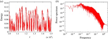
In the non-rotating case, figure 6 shows the time development of the energy of the unsteady solutions and its power spectrum. The energy changes irregularly and its power spectrum is broad. The unsteady solution is seemingly chaotic, and the time-averages of some quantities in the time interval of
 $5\times 10^{4}\leqslant t\leqslant 5\times 10^{5}$
are robust among some numerical solutions from different series of random numbers.
An example of the time development of the energy of the chaotic solutions (a) and its power spectrum (b). In (a) the horizontal and vertical axes indicate the time and the energy, while in (b) the horizontal and vertical axes indicate the frequency and the power spectrum.

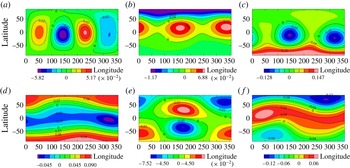
Figure 7 shows the time series of the streamfunction of the unsteady solution, while the streamfunction of the steady-travelling solutions at
 $\mathit{Re}=10^{4}$
is represented in figure 8. The streamfunctions at some instants of the unsteady solution are similar to those of the unstable steady solutions. This observation suggests that the orbit of the unsteady solution wanders around the steady and steady-travelling solutions. Moreover, the unsteady solution is not highly but moderately turbulent, and therefore we expect that the orbit of the unsteady solution is mostly located in a low-dimensional space spanned by the steady and steady-travelling solutions.
Snapshots of the streamfunction of a chaotic solution at
 ${\it\Omega}=0$
and
 $\mathit{Re}=10^{4}$
: (a)
 $t=107\,000$
, (b)
 $t=108\,000$
, (c)
 $t=146\,000$
, (d)
 $t=182\,000$
, (e)
 $t=237\,000$
and ( f)
 $t=313\,000$
, respectively. The horizontal and vertical axes indicate longitude and latitude. Panels (a–c,e,f), respectively, resemble
 $S_{1}$
,
 $S_{11}^{l}$
,
 $S_{12}^{u}$
,
 $S_{21}^{u}$
,
 $S_{2}$
and
 $S_{21}^{l}$
in figure 8.

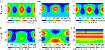
The streamfunctions of the steady-travelling solutions at
 ${\it\Omega}=0$
and
 $\mathit{Re}=10^{4}$
: (a)
 $S_{1}$
, (b) the lower branch of
 $S_{11}$
, (c) the lower branch of
 $S_{12}$
, (d) the lower branch of
 $S_{121}$
, (e)
 $S_{2}$
, and ( f) the lower branch of
 $S_{21}$
. The horizontal and vertical axes indicate longitude and latitude. The lower branches of
 $S_{11},S_{12},S_{121}$
and
 $S_{21}$
have the equatorial anti-symmetric relation with its upper branch.

However, because the system is invariant to the longitudinal translation, even the set of steady solutions constitutes an infinite-dimensional linear space, which is difficult to approximate by numerical calculations. Therefore we focus our attention on the zonal-mean zonal flows instead of the 2D flow field. The former flow is defined as
 $$\begin{eqnarray}\boldsymbol{U}({\it\mu})=\frac{1}{2{\rm\pi}}\int _{0}^{2{\rm\pi}}\hspace{2.22198pt}u_{{\it\lambda}}({\it\lambda},{\it\mu})\hspace{2.22198pt}\text{d}{\it\lambda},\end{eqnarray}$$
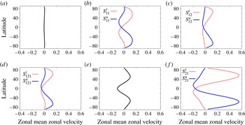
which eliminates the infinite dimension arising from the longitudinal translation. In figure 9 we plot the zonal-mean zonal velocity of these solutions at
 $\mathit{Re}=10^{4}$
. The solution
 $S_{1}$
has a symmetry group generated by
 ${\it\Sigma}_{{\rm\pi}/2}^{-}$
, but
 $S_{1}$
and
 ${\it\Sigma}_{{\rm\pi}/2}^{-}S_{1}$
give the same zonal-mean zonal velocity profile, and so does
 $S_{2}$
. Each of the other solutions, however, gives two zonal-mean zonal velocity profiles when the symmetry is taken into account. In total, therefore, 11 independent velocity profiles, including the trivial zonal flow, are obtained from these solutions.
The zonal-mean zonal velocity of the steady-travelling solutions at
 ${\it\Omega}=0$
and
 $\mathit{Re}=10^{4}$
: (a)
 $S_{1}$
, (b)
 $S_{11}$
, (c)
 $S_{12}$
, (d)
 $S_{121}$
, (e)
 $S_{2}$
, and ( f)
 $S_{21}$
. Both these solutions are Hopf unstable at
 $\mathit{Re}=249.5$
.

We try to reproduce the zonal-mean zonal velocity profile of the unsteady solution using a linear combination of the 11 unstable steady and steady-travelling solutions.
First, a linear space
 $M$
spanned by the 11 unstable steady and steady-travelling solutions is introduced, and an orthogonal projection
 $P_{M}({\it\psi})$
from the unsteady solution
 ${\it\psi}$
to
 $M$
is defined. Further,
 $Z({\it\psi})$
is defined as a mapping from
 ${\it\psi}$
to the zonal-mean zonal velocity of
 ${\it\psi}$
. Therefore, when
 $Z(P_{M}(\cdot ))$
operates on a general streamfunction, it gives a linear combination of the zonal-mean zonal velocity of the 11 solutions. The orthogonal projection,
 $P_{M}({\it\psi})=\hat{{\it\psi}}({\it\lambda},{\it\mu},t)$
, is expressed as
 $$\begin{eqnarray}\hat{{\it\psi}}({\it\lambda},{\it\mu},t)=\mathop{\sum }_{k=1}^{K}\int \frac{\text{d}{\it\theta}}{2{\rm\pi}}c_{k}({\it\theta},t){\it\psi}_{k}({\it\lambda}-{\it\theta},{\it\mu})+d(t){\it\psi}^{T}({\it\mu}),\end{eqnarray}$$
where
 ${\it\psi}_{k}({\it\lambda},{\it\mu})(k=1,\dots ,K)$
are the unstable steady and steady-travelling solutions which depend on both the longitude and the latitude,
 ${\it\psi}^{T}({\it\mu})$
is the trivial solution and
 $c_{k}({\it\theta},t)$
and
 $d(t)$
are coefficients. The zonal velocity profile of the streamfunction projected on
 $M$
,
 $Z(P_{M}({\it\psi}))=\hat{\boldsymbol{U}}({\it\mu},t)$
, is then given by
 $$\begin{eqnarray}\hat{\boldsymbol{U}}({\it\mu},t)=\mathop{\sum }_{k=1}^{K}\int \frac{\text{d}{\it\theta}}{2{\rm\pi}}c_{k}({\it\theta},t)\boldsymbol{U}_{k}({\it\mu})+d(t)\boldsymbol{U}^{T}({\it\mu}),\end{eqnarray}$$
where
 $\boldsymbol{U}_{k}({\it\mu})=Z({\it\psi}_{k})$
and
 $\boldsymbol{U}^{T}({\it\mu})=Z({\it\psi}^{T})$
, respectively. The coefficients
 $\int (\text{d}{\it\theta}/2{\rm\pi})c_{k}({\it\theta},t)$
and
 $d(t)$
are given by
 $$\begin{eqnarray}\int \frac{\text{d}{\it\theta}}{2{\rm\pi}}c_{k}({\it\theta},t)=\int _{-1}^{1}\frac{\text{d}{\it\mu}}{2}\boldsymbol{U}_{k}^{\dagger \ast }({\it\mu})\boldsymbol{U}({\it\mu},t),\quad d(t)=\int _{-1}^{1}\frac{\text{d}{\it\mu}}{2}\boldsymbol{U}^{T\dagger \ast }({\it\mu})\boldsymbol{U}({\it\mu},t),\end{eqnarray}$$
where
 $\{\boldsymbol{U}_{k}^{\dagger }({\it\mu}),\boldsymbol{U}^{T\dagger }({\it\mu})\}\;(k=1,\dots ,K)$
denotes the dual basis of
 $\{\boldsymbol{U}_{k}({\it\mu}),\boldsymbol{U}^{T}({\it\mu})\}\;(k=1,\dots ,K)$
,
 $\boldsymbol{U}({\it\mu},t)=Z({\it\psi})$
, and
 $\text{}^{\ast }$
indicates complex conjugate.
The dual vectors
 $\{\boldsymbol{U}_{i}^{\dagger }({\it\mu})\}$
to a set of vectors
 $\{\boldsymbol{U}_{i}({\it\mu})\}$
are constructed so that the inner product of
 $\boldsymbol{U}_{i}({\it\mu})$
and
 $\boldsymbol{U}_{j}^{\dagger }({\it\mu})$
is
 ${\it\delta}_{ij}$
. The vectors
 $\{\boldsymbol{U}_{i}({\it\mu})\}$
are observed to be linearly independent, and therefore the dual vectors
 $\boldsymbol{U}_{i}^{\dagger }({\it\mu})$
are obtained by using Gram–Schmidt orthogonalization on the assumption that the dual vectors
 $\{\boldsymbol{U}_{i}^{\dagger }({\it\mu})\}$
belong to the linear space spanned by
 $\{\boldsymbol{U}_{i}({\it\mu})\}$
.
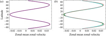
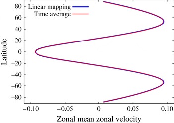
Figure 10(a) shows the time-average of the reproduced zonal-mean zonal velocity. We find that the reproduced velocity profile agrees well with that of the unsteady solution within
 ${\sim}1.1\,\%$
error. Further, figure 10(b) shows the time-averages of the reproduced zonal-mean zonal velocity using only the trivial solution and only the single pair of
 $S_{21}$
. Even when only the single solution and the pair of
 $S_{21}$
are employed, the reproduced velocity and the time-averaged zonal velocity profile agree well with each other.
The reproduced zonal-mean zonal velocity by the linear mapping: (a) the 11 steady and steady-travelling solutions, and (b) the trivial solution/the single pair of
 $S_{21}$
. The red lines show the time-averaged zonal-mean zonal velocity profile of the unsteady flow, the blue lines the reproduced profiles using 11 steady and steady-travelling solutions, the green lines using only the trivial solution and the light blue lines using the pair of
 $S_{21}$
solutions. The reproduced profile agrees well with that of the unsteady solution.

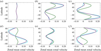
Figure 11 shows the reproduced zonal-mean zonal velocity profiles and the unsteady flow at several times. There are significant errors between the zonal-mean zonal velocity profiles of the unsteady solutions and the reproduced profiles, unless the 11 solutions are employed for the reproduction of which the relative error is of the order of 0.01 %.
The instantaneous zonal-mean zonal velocity profiles and the reproduced profiles at the same times as in figure 7. The red lines show the zonal-mean zonal velocity profile of the unsteady flow, the blue lines the reproduced profiles using 11 steady and steady-travelling solutions, the green lines using only the trivial solution and the light blue lines using the pair of
 $S_{21}$
solutions.

These results suggest that even at high Reynolds numbers (
 ${\sim}40$
times that of the critical Reynolds number of the laminar flow), the unsteady solution mostly lies within the relatively low-dimensional space spanned by the steady and steady-travelling solutions which bifurcate at low Reynolds numbers.
We examine each projected component of
 $\hat{\boldsymbol{U}}({\it\mu},t)$
to the steady and steady-travelling solution,
 $$\begin{eqnarray}\int \frac{\text{d}t}{T}\left(\int _{-1}^{1}e_{i}^{\ast }({\it\mu})\hat{\boldsymbol{U}}({\it\mu},t)\frac{\text{d}{\it\mu}}{2}\right)^{2},\end{eqnarray}$$
where
 $e_{i}({\it\mu})$
is a normalized unit vector of the dual basis
 $\boldsymbol{U}_{i}^{\dagger }({\it\mu})$
. This quantity represents the amount of the contribution of
 $\boldsymbol{U}_{i}({\it\mu})$
to
 $\hat{\boldsymbol{U}}({\it\mu},t)$
. We exclude
 $\boldsymbol{U}_{i}({\it\mu})$
giving the smallest contribution and then again perform a reproduction using the remaining 10 solutions. By repeating this procedure, we successively reduce the number of the solutions
 $\boldsymbol{U}_{i}({\it\mu})$
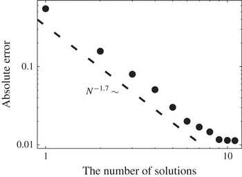
for the reproduction. Figure 12 shows the absolute error
 $$\begin{eqnarray}\int \frac{\text{d}t}{T}\sqrt{\int _{-1}^{1}\frac{\text{d}{\it\mu}}{2}(\boldsymbol{U}({\it\mu},t)-\hat{\boldsymbol{U}}({\it\mu},t))^{2}}\end{eqnarray}$$
against the number
 $N$
of steady and steady-travelling solutions employed for the production. We see that when the 11 solutions are employed, the absolute error is smallest, but as the number of solutions decreases, the absolute error increases as
 $N^{-1.7}$
.
The absolute error and the number of solutions used for the reproduction. The dashed line shows
 $N^{-1.7}$
, where the exponent
 $-1.7$
is obtained by the least-squares method in the range
 $1\leqslant N\leqslant 8$
.

Let us assume the attractor of the unsteady solution uniformly distributes in the
 $M$
-dimensional sphere with radius
 $r_{c}$
. The distance between this attractor and the subspace spanned by the
 $N$
mutually orthogonal vectors
 $(N<M)$
is then given by
 $d_{N}=\sqrt{\int _{V_{M}}(\text{d}V/V_{M})\sum _{i=1}^{M-N+1}x_{i}^{2}}=\sqrt{(M-N+1)/(M+2)}r_{c}$
, where
 $V_{M}$
is the volume of the
 $M$
-dimensional sphere. The absolute error is therefore proportional to
 $\sqrt{12-N}$
, which is in contrast with
 $N^{-1.7}$
in our case. This result suggests that the attractor of the unsteady solution distributes non-uniformly.
We also carried out the time integration in the rotating cases,
 ${\it\Omega}=\pm 1.0$
, at high Reynolds numbers, and the unsteady solutions are either time-periodic or stable steady (not chaotic), suggesting the stabilizing effect of the rotation. Here we show the representative result of
 ${\it\Omega}=-1.0$
and
 $\mathit{Re}=10^{3}$
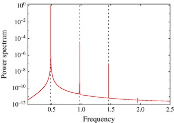
. Figure 13 shows the power spectrum in this case and the unsteady solution is time-periodic.
The power spectrum of the energy of the time-periodic solutions at
 ${\it\Omega}=-1.0$
and
 $\mathit{Re}=10^{3}$
. The horizontal and vertical axes indicate the frequency and the power spectrum. The vertical dashed lines indicate
 ${\it\omega}=0.487$
,
 $2{\it\omega}$
and
 $3{\it\omega}$
, respectively.

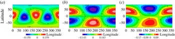
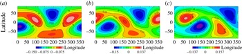
Figure 16 shows snapshots of streamfunction of the time-periodic solution. For comparison we show the streamfunctions of four steady-travelling solutions at
 $\mathit{Re}=10^{3}$
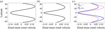
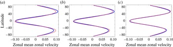
in figure 14, while figure 15 shows their zonal-mean zonal velocity profiles. The flow field of the time-periodic solution is not similar to those of steady-travelling solutions. We reproduced the zonal-mean zonal velocity profiles using the five steady and steady-travelling solutions (figure 17). There are some discrepancies between the reproduced profiles and the time-periodic solution. However, the time-averaged zonal-mean zonal velocity can be successfully reproduced, as shown in figure 18. This result suggests that even the time-periodic solutions are not far from the unstable steady and steady-travelling solutions.
The streamfunction of the steady-travelling solutions at
 ${\it\Omega}=-1.0$
and
 $\mathit{Re}=10^{3}$
: (a)
 $S_{1}$
, (b)
 $S_{2}$
, (c)
 $S_{25}^{l}$
. The horizontal and vertical axes indicate longitude and latitude.

The zonal-mean zonal velocity of the steady-travelling solutions at
 ${\it\Omega}=-1.0$
and
 $\mathit{Re}=10^{3}$
: (a)
 $S_{1}$
, (b)
 $S_{2}$
, (c)
 $S_{25}$
. The horizontal and vertical axes indicate amplitude and latitude.

Snapshots of the streamfunction of the time-periodic solution at
 ${\it\Omega}=-1.0$
and
 $\mathit{Re}=10^{3}$
: (a)
 $t=400\,291$
, (b)
 $t=400\,294$
, (c)
 $t=400\,298$
. The horizontal and vertical axes indicate longitude and latitude.

Snapshots of the zonal-mean zonal velocity of the time-periodic solution at
 ${\it\Omega}=-1.0$
and
 $\mathit{Re}=10^{3}$
. The distributions are shown at the same times as in figure 16. The red and blue (thin and thick) lines indicate the time-periodic solution and reproduced profiles using the linear mapping constructed with all four steady and steady-travelling solutions. The horizontal and vertical axes indicate velocity and latitude.

The time-averaged zonal-mean zonal velocity and reproduced profile at
 ${\it\Omega}=-1.0$
and
 $\mathit{Re}=10^{3}$
. The red and blue (thin and thick) lines represent the time-periodic solution velocity profiles reproduced by the linear mapping constructed with all four steady and steady-travelling solutions. The horizontal and vertical axes indicate velocity and latitude.

On the other hand, in the case of
 ${\it\Omega}=1.0$
, all the unsteady solutions converge to
 $S_{11}$
at
 $\mathit{Re}=10^{3}$
, while most of the unsteady solutions except in a neighbourhood of
 $S_{11}$
are time-periodic at
 $\mathit{Re}=10^{4}$
.
6. Discussion and conclusions
In this paper we have studied the bifurcation structure of viscous zonal flows on a rotating sphere under zonal forcings. Our problem could be considered as an extension of the Kolmogorov problem on a flat torus.
We prove rigorously that two-jet zonal flow is globally stable for an arbitrary Reynolds number and an arbitrary rotation rate. We note that in the flat torus case, Iudovisch (Reference Iudovisch1965) proved that two-jet parallel flow is globally asymptotically stable for arbitrary Reynolds number.
Next we studied the bifurcation structure of nonlinear steady solutions arising from three-jet zonal flow. In the non-rotating case, as the Reynolds number increases, the steady-travelling solutions arise from three-jet zonal flow via Hopf bifurcations. As the Reynolds number increases further, several travelling solutions arise only via pitchfork bifurcation, and finally the steady-travelling solutions become Hopf unstable. In the rotating case, on the other hand, we find saddle-node bifurcations, closed-loop branches and linearly stable solutions at high Reynolds numbers. Thus the bifurcation structure changes drastically under the effect of rotation. On the flow field of the steady-travelling solutions, in the non-rotating case, we find equatorial symmetry restoration of the steady-travelling solution at high Reynolds numbers. In the flat torus case, Okamoto & Shōji (Reference Okamoto and Shōji1993) and Kim & Okamoto (Reference Kim and Okamoto2010) found steady solutions for which the flow field is dominated only by one pair of negative and positive vortices at high Reynolds numbers. It should be noticed that the symmetries of those steady solutions are also restored as the Reynolds number increases. In the rotating cases, on the other hand, we do not find symmetry restoration of the steady-travelling solutions. We note that the rotation of the system further introduces the resonant interaction of the spherical harmonics, i.e. Rossby waves, in the flow system, and makes its analysis more complicated at moderate rotation rates, while the dynamics at extremely high rotation rates (Kartashova & L’vov Reference Kartashova and L’vov2008) would be modelled by taking into account only the resonant interaction of spherical harmonics. We also note that it would be interesting to make a low-dimensional model system of the turbulent state by taking appropriate spherical harmonics to get insight into the physical mechanism of the turbulence which appears to be a low dimension.
We carry out the time integration of the equation of motion at high Reynolds numbers where the steady and steady-travelling solutions are Hopf unstable. In the non-rotating case, we observed that the unsteady solutions goes around the unstable steady-travelling solutions. We reproduce the zonal-mean zonal velocity of the unsteady solution using a linear combination of those of the steady and steady-travelling solutions. We find that the reproduction of the zonal-mean zonal profiles approximates those of the unsteady solutions well. This result suggests that even at high Reynolds numbers the chaotic attractor exists mostly within a relatively low-dimensional space spanned by the steady and steady-travelling solutions.
Recently, low-dimensional ODE models of wall turbulence have been studied in order to understand the turbulence dynamics (Smith, Moehlis & Holmes Reference Smith, Moehlis and Holmes2005; Kim & Moehlis Reference Kim and Moehlis2008). In this paper we show that a low-dimensional space constructed by the steady and steady-travelling solutions gives a good approximation in the case of 2D high-Reynolds number flows on a rotating sphere. It would be interesting to see if an attractor is found near steady or similar simple solutions in 3D cases.
Acknowledgements
We would like to express our deepest gratitude to Professor H. Okamoto for the fruitful discussions. In the numerical calculation of the spectrum method we use the spectral transformation library ‘ISPACK’ (Ishioka Reference Ishioka2011) and the FORTRAN90 wrapper library ‘SPMODEL’ (Takehiro et al. Reference Takehiro, Sasaki, Morikawa, Ishioka, Odaka, Takahashi, Nishizawa, Nakajima, Ishiwatari and Hayashi2011). This work was supported by JSPS KAKENHI grants 24340016, 15K13458 and 25610139 and MEXT KAKENHI grant 26103706.