NOMENCLATURE
- A p
-
cross-sectional area of particle
- A s
-
surface area of particle
- A ⊥
-
projected area of the particle with respect to the flow
- B, h
-
ice and water layer thicknesses
- C D
-
drag coefficient of cloud particle
- C p
-
specific heat at constant pressure
- CS
-
Certification Specification
- d p
-
particle diameter
- D
-
diffusivity
- D
-
drag force of cloud particle
- e
-
particle eccentricity
- e σ
-
surface energy per unit area
- E
-
particle aspect ratio
- EASA
-
European Aviation Safety Agency
- FAA
-
Federal Aviation Administration
- FAR
-
Federal Aviation Regulation
- g
-
gravitational acceleration
- h t
-
heat transfer coefficient
- HAIC
-
High Altitude Ice Crystals
- k
-
thermal conductivity
- k s
-
roughness height
- L f , L v
-
latent heat of freezing and evaporation
- L
-
ratio of the kinetic energy to surface energy
-
 $\dot{m}$
-
mass flow rate
- m p
-
mass of cloud particle
- M
-
molar masses
- MMD
-
mean mass diameter
- MVD
-
mean volumetric diameter
- Nu
-
Nusselt number
- NASA
-
National Aeronautics and Space Administration
- P B P D
-
particle bouncing and deposition probabilities
- P
-
pressure
- Pr
-
Prandtl number
- Q
-
heat terms in the interface conditions as explained in the text
- Q s
-
activation energy
- r
-
sticking efficiency of cloud particle
- r p
-
particle radius
- Re
-
Reynolds number
- Re k
-
roughness Reynolds number
- RH
-
relative humidity
- s
-
circumferential distance along the geometry surface
- Sc
-
Schmidt number
- Sh
-
Sherwood number
- St
-
Stanton number
- t
-
time
- T
-
temperature in the ice layer
- TUBS
-
Technical University of Braunschweig
- U e
-
edge velocity
- U k
-
flow velocity at the roughness location
- v p
-
particle volume
- V rel
-
particle relative velocity
- V ∞
-
freestream velocity
- V x , V y
-
velocity vector components of the flow field
- V
-
velocity magnitude of cloud particle with respect to the flow field
- x, y
-
Cartesian coordinates
-
$\ddot{x}_p, \ddot{y}_p$
-
acceleration vector components of the cloud particle
-
$\dot{x}_p, \dot{y}_p$
-
velocity vector components of the cloud particle
- x p , y p
-
position vector components of the cloud particle
- y v
-
vapour mass fraction
- α melt
-
melt ratio of ice crystals after impinging
- β
-
local collection efficiency
- γ
-
angle between velocity vectors of the cloud particle and flow field
- δ
-
boundary-layer thickness
- ε er
-
erosion rate
- ε s
-
particle sticking efficiency
- ζ
-
particle restitution coefficient
- η melt
-
melt ratio of ice crystals before impinging
- θ
-
temperature in the water layer or momentum thickness
- λ
-
energy terms in the energy balance equation
- μ
-
dynamic viscosity
- ν
-
kinematic viscosity
- χ
-
evaporation or sublimation coefficient
- ϕ
-
particle sphericity
- ϕ⊥
-
particle crosswise sphericity
- ψ c
-
impinging crystal mass to impinging total mass ratio
- ψ l
-
impinging droplet mass to impinging total mass ratio
- ρ
-
density of air or liquid water content
- σ w
-
surface tension of water
- τ
-
shear stress
- a
-
air properties
- c, l
-
quantities related to solid (crystal) or liquid (droplet) cloud particles
- con
-
quantities related to convection
- ct
-
constant
- ev
-
quantities related to evaporation
- f
-
quantities related to freezing
- i
-
ice properties
- imp
-
quantities related to impinging particles
- in
-
quantities related to inflowing runback water
- k
-
airflow properties at roughness height
- lam
-
laminar flow
- m
-
mixture properties
- n
-
normal component
- p
-
particle
- r, g
-
quantities related to rime or glaze ice
- rec
-
recovery
- ref
-
reference
- s
-
quantities related to sticking ice crystals, static
- sat
-
saturated air properties
- sub
-
quantities related to sublimation
- subs
-
substrate
- tang
-
tangential
- t
-
tangential component
- tr
-
transition
- turb
-
turbulent
- v
-
vapour properties
- w
-
water properties


Greek Symbol
Subscript
1.0 INTRODUCTION
Ice accumulation on aircraft components during flight is one of the most severe threats to flight safety. Icing on wings, stabilising surfaces, control surfaces, engine components and flight data sensors may result in degradation of aerodynamic performance, alteration of stability and control characteristics often in an unpredictable manner, severe reduction in engine performance, false flight data readings and increase in weight. Therefore, transport category aircraft must demonstrate that they can fly safely in icing conditions by complying with airworthiness requirements issued by Certification Authorities. These conditions and related requirements are included in FAR-25 (Federal Aviation Administration (FAA)) and CS-25 (European Aviation Safety Agency (EASA)).
For a long time and until very recently, icing conditions and related requirements were covered by Appendix C, which takes into account only the icing conditions involving liquid phase clouds and where the cloud droplets are smaller than 50 microns. However, following the review of icing related events, Ice Protection Harmonization Working Group (IPHWG) found accidents and incidents that were believed to have occurred in icing conditions that were not addressed by Appendix C. There have also been a number of power loss event reports during the last two decades, which have occurred in the presence of ice crystals and mixed phase conditions. Some of these events involved multi-engine power loss. Although the events did not result in accidents, they were considered as serious safety threats. Therefore, it was proposed to amend CS-25 and FAR-25 to better protect large aircraft certified for flight in icing conditions(9). As a result, both FAA(11) and EASA(10) have issued amendments to their respective certification regulations extending the icing envelopes to include Supercooled Large Droplets-SLD and mixed phase clouds in Appendix O and Appendix P (Appendix D in FAR-25), respectively.
High water content is often encountered in deep convective clouds present in tropical regions. Updraft cores of these clouds continuously transport humid air at low-level to higher altitudes, where water vapour is condensed as the temperature decreases. As a result, there may be regions in the clouds with very high ice crystal concentration and also where ice crystals and liquid water droplets may co-exist. Ice accretion in such conditions involve phenomena that are significantly more complex than those in Appendix C icing conditions(Reference Villedieu, Trontin and Chauvin30). Some of these phenomena are trajectories of non-spherical ice crystals, heat transfer and melting in ice crystals, impingement of ice particles on a dry or wet surface, re-emission of ice particles from the surface after impact and erosion.
Mason et al(Reference Mason, Strapp and Chow21) describe an engine icing incidence. Ice crystals first melt upon contact with warm engine parts and a water film is created. Subsequent ice particles are captured by the water film allowing ice accumulation to occur. The engine abnormalities then occur when this ice buildup sheds.
The study of Nilamdeen et al(Reference Nilamdeen, Habashi, Aubé and Baruzzi23) is among the early numerical attempts to address mixed phase icing by solving the governing equations for multiphase flow. Emphasis has been given to ice crystal drag coefficient modelling and crystal bouncing. Four mixed phase ice accretion cases experimented in the Cox icing tunnel were studied.
The study of Wright et al(Reference Wright, Jorgenson and Veres32) extends the GlennICE numerical tool to model mixed-phase conditions. The study mentions the modifications that were made to GlennICE including those related to the particle trajectory algorithm, energy balance and erosion. The same four test cases as in Nilamdeen et al’s study are investigated, together with an engine ice ingestion case.
A comprehensive account of mixed phase and glaciated icing conditions and their numerical modelling has been given by Villedieu et al(Reference Villedieu, Trontin and Chauvin30) and Trontin et al(Reference Trontin, Blanchard and Villedieu28). These studies give a detailed account of models related to particle trajectories, heat transfer and phase change, impingement, accretion and erosion related to mixed phase accretion. Calibrations of model parameters are also explained in a detailed manner.
The experimental work of Al-Khalil et al(Reference Al-Khalil, Irabi and Miller1) and the results therein have become benchmarks for the validation of computational results related to mixed phase icing. The authors present the results of wind-tunnel tests under liquid phase and mixed phase conditions at the Cox wind tunnel. Four of these experimental cases have been extensively used by icing researchers developing numerical tools worldwide for validation. These cases are also studied in the present study for validating the results of the current computational tool.
More recent experimental efforts have been reported by Currie et al(Reference Currie, Fuleki, Knezevici and MacLeod6-Reference Currie, Struk, Tsao, Fuleki and Knezevici8). These references include databases obtained in the National Research Council of Canada wind tunnel and have been used by Villedieu et al(Reference Villedieu, Trontin and Chauvin30) and Trontin et al(Reference Trontin, Blanchard and Villedieu28) to develop the models related to mixed phase icing, most of which are used in the current study as well.
The current study is focused on the two-dimensional numerical analysis of ice accretion in mixed phase conditions, where models related to mixed phase icing are implemented to an existing in-house tool. The numerical tool has four modules; a flow-field solution module that uses the Hess-Smith panel method, a module for computing droplet and ice crystal trajectories and collection efficiencies using the Lagrangian approach, a thermodynamical module, and an ice accretion module that utilises the Extended Messinger Model. The Extended Messinger Model has been introduced by Myers(Reference Myers22) as a significant improvement over the Original Messinger Model. A major improvement is the introduction of temperature gradients in the ice and water layers instead of fixed temperatures resulting in an unrealistic temperature discontinuity in the ice/water interface. In the Extended Messinger Model, transition from rime ice to glaze ice is smooth, whereas it is sudden in the Original Messinger Model. These two improvements render the Extended Messsinger Model a more faithful representation of the icing physics. The Extended Messinger Model has been used extensively by the present authors to study icing in liquid phase cloud conditions for aerofoil, wing and intake geometries, and the obtained results have been validated(Reference Özgen and Canıbek24,Reference Özgen and Canıbek25) . In the present study, Extended Messinger Model has been modified further to include mixed phase effects together with the relevant models: drag coefficient models, heat transfer and phase change models for ice crystals and water droplets in trajectory calculations, impingement models and erosion models.
These efforts were undertaken within the context of the High Altitude Ice Crystals (HAIC) project, funded by the European Commission within Framework Program 7, where Turkish Aerospace Industries is a partner.
2.0 PROBLEM FORMULATION AND SOLUTION METHOD
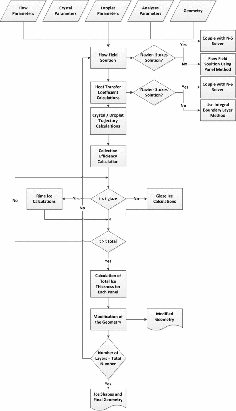
In this section, the formulation of the ice accretion problem and the solution method are introduced. The flowchart of the developed computational tool is presented in Fig. 1.
Flowchart of the mixed phase ice accretion prediction tool, TAICE.

2.1 Flow field solution: Hess-Smith panel method
Two-dimensional Hess-Smith panel method is used to determine the flow velocity components required for droplet trajectory calculations and the velocity distribution around the aerofoil for boundary-layer calculations. The aerofoil is divided into quadrilateral panels, each having a constant strength source singularity element plus a vortex singularity that is constant for all panels. Using the flow tangency boundary condition at the collocation points of the surface panels, the singularity strengths are obtained. This provides the velocity potential at any point in the flow field. The derivatives of the velocity potential are the velocity components at a given point in the flow field. Moreover, integral boundary-layer method is used in TAICE for calculating heat transfer coefficients when they are not supplied with another tool. Since equations which are used for calculating heat transfer coefficients depend on the flow being laminar or turbulent, transition prediction should be considered. The method which is used for the calculation of these coefficients are given in well-known references(Reference Gent, Dart and Cansdale13,Reference Schlicting27) .
2.2 Particle trajectory calculations
The equations governing droplet and crystal trajectories are identical. However, the models used for drag force and heat transfer predictions differ depending on the phase of cloud particles. The differences are pointed out below, where appropriate. The following assumptions are made for the particles:
-
• The presence of cloud particles has no effect on the flowfield,
-
• Gravity and aerodynamic drag are the only forces acting on the cloud particles.
Thus, the governing equations for particle motion in Cartesian coordinates are(Reference Myers22):
 $$\begin{equation}
m_p\ddot{x} = -D \cos {\gamma }, \\
\end{equation}$$
 $$\begin{equation}
m_p\ddot{y} = -D \cos {\gamma }+mg, \\
\end{equation}$$
 $$\begin{equation}
\gamma = \arctan \frac{\dot{y}_p-V_y}{\dot{x}_p-V_x}, \\
\end{equation}$$
 $$\begin{equation}
D = \frac{1}{2} \rho V^2 C_D A_p, \\
\end{equation}$$
 $$\begin{equation}
V = \sqrt{\left(\dot{x}_p-V_x\right)^2+\left(\dot{y}_p-V_y\right)^2}.
\end{equation}$$
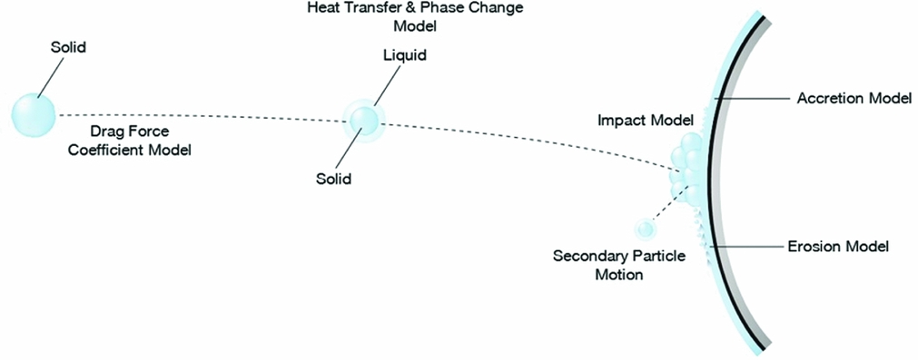
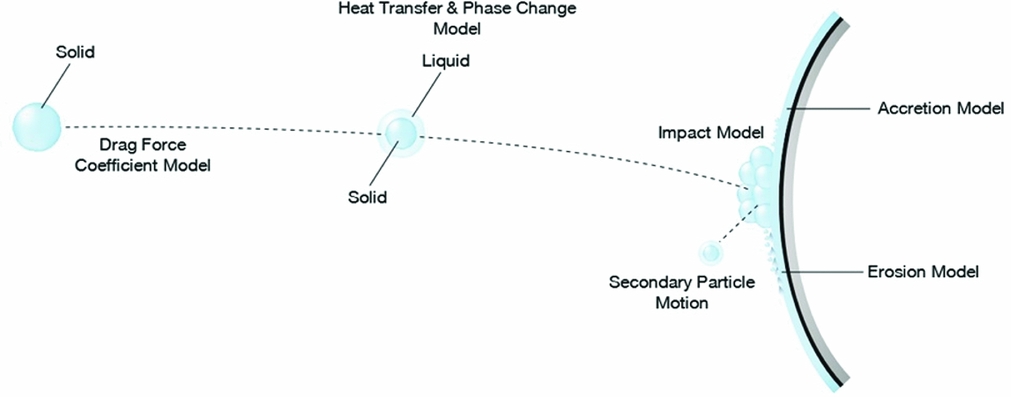
In the above expressions, C D is drag force coefficient, and V x and V y are velocity components of the particle. Calculation of the drag coefficient depends on the particle type. Ice crystals are formed generally within the tropical clouds and may have various shapes. They differ from liquid droplets in terms of their shape and usually are not exactly spherical. Thus, for accurate prediction of the trajectories, drag force coefficient, heat transfer and phase change models should be modified for non-spherical particles in order to be used for ice crystals. Required models are depicted along the trajectory shown in Fig. 2. Brief explanations about the trajectory models are given in section A of the Appendix. More detailed information can be found in the studies of Trontin et al, Villedieu et al(Reference Trontin, Blanchard and Villedieu28,Reference Villedieu, Trontin and Chauvin30) and Ayan et al(Reference Ayan, Özgen and Canıbek2).
Models related to mixed phase icing starting from the release point till accretion on the surface.
2.3 Impingement model for ice crystals
Impinging ice crystals on a surface may lead to three different scenarios which are sticking, bouncing and shattering. Impact model which is discussed in this section is mainly based on HAIC experiments and literature data(Reference Trontin, Blanchard and Villedieu28,Reference Villedieu, Trontin and Chauvin30) . A brief information will be given here about these regimes.
In bouncing and sticking regimes, particle size and shape do not change after impact. However, it may split into smaller particles in the shattering regime. In the bouncing regime, particles just bounce off from the wall and are re-emitted to the flow. On the other hand, in sticking regime, particles adhere to the wall completely. The threshold between these regimes depends on the kinetic energy of the particle before impact. Below, a dimensionless number L, which is the ratio of the kinetic energy to the surface energy of the particle, is introduced(Reference Trontin, Blanchard and Villedieu28,Reference Villedieu, Trontin and Chauvin30) .
 $$\begin{eqnarray}
L=\frac{1}{12}\frac{\pi \rho _p d_p^{3}v_{pn}^{2}}{\pi e_\sigma T_p d_p^{2}}=\frac{1}{12}\frac{\rho _p d_p v_{pn}^{2}}{e_\sigma T_p} ,
\end{eqnarray}$$
In the above equation, v pn is the normal velocity of the particle and e σ is the surface energy per unit area and can be calculated with the following relation:
 $$\begin{eqnarray}
e_\sigma =e_{\sigma 0}\exp \left(\frac{Q_s}{RT}-\frac{Q_s}{RT_0}\right),\vspace*{-5pt}
\end{eqnarray}$$
where Q s is the activation energy. As it is given in Higa et al(Reference Higa, Arakawa and Maeno18), Q s = 4.82 × 10 4 J K−1.mol−1 and according to the Vidaurre and Hallet(Reference Vidaurre and Hallett29) e σ0 = 0.12 J.m−2 at T 0 = 253 K.
Thus, when L ⩾ 90, high loss of kinetic energy and high fragmentation occurs upon impact; when L ⩽ 0.5, no fracturing is expected. On the other hand, when L is in between these values, inelastic bouncing with some particle fragmentation is expected. However, less kinetic energy loss will occur in this case. These values are determined based on both literature data(Reference Hauk, Roisman and Tropea17) and Hauk’s experimental results(Reference Hauk, Roisman and Tropea17).
Predicting sticking ratio is the challenging part of this model and a simple relation is suggested by Trontin et al(Reference Trontin, Blanchard and Villedieu28). In their study, sticking ratio depends only on the mean melt ratio of the impinging ice crystals and total water content of the flow. The model is calibrated using the National Aeronautics and Space Administration and National Research Council of Canada (NASA - NRC) experiments(Reference Currie, Fuleki, Knezevici and MacLeod6-Reference Currie, Struk, Tsao, Fuleki and Knezevici8). However, in this study, a more simplified form of their relation is used:
 $$\begin{eqnarray}
\epsilon _s&=&K_l\psi _l\vspace*{-5pt}
\end{eqnarray}$$
In the above equation, sticking ratio is related to the dimensionless parameter, K l , and the liquid ratio of the impinging particles, ψ l . According to Trontin et al(Reference Trontin, Blanchard and Villedieu28), in rime ice conditio,n ice crystals do not stick on the surface and K l should be equal to zero for consistency. Moreover, after calibration study, K l is fixed to 2.25 for glaze ice conditions.
Impinging liquid and solid ratios in total amount of impinging particles are given below.
 $$\begin{equation}
\psi _l = \frac{\dot{m}_{imp,l}}{\dot{m}_{imp,c}+\dot{m}_{imp,l}} \\
\end{equation}$$
 $$\begin{equation}
\psi _c = \frac{\dot{m}_{imp,c}}{\dot{m}_{imp,c}+\dot{m}_{imp,l}}
\end{equation}$$
Moreover, it is observed from the experiments that the sticking ratio of the ice crystals increases with increasing ψ l up to a threshold value. However, further increase does not cause additional increase in the sticking ratio of the ice crystals. Thus, a limitation is introduced here for ψ l for this purpose. Its value could not exceed 0.2, which is determined during the calibration study.
In addition, the model predicts behaviour of secondary particles which are produced in case of bouncing or shattering regimes. The model is mainly empirical and the adjustable constant has been fitted thanks to literature and HAIC experimental data.
Since bouncing ice crystal particles may re-impinge and accumulate in downstream, their trajectory calculations should be continued after impact. Relations which are used for modelling these secondary particle behaviours can be found in Refs 2 and 28.
2.4 Erosion Model
It is observed in experiments that in mixed phase icing conditions, upcoming solid particles cause reduction in the amount of accreted ice on the surface(Reference Al-Khalil, Irabi and Miller1). Generally, this reduction is much more noticeable in glaze ice conditions. Wright et al(Reference Wright, Jorgenson and Veres32) proposed a model for prediction of erosion effect. In this study, this model is modified by using additional available experimental data. A modified version of the model is given below which is used to predict erosion effect on accreted ice.
 $$\begin{eqnarray}
\epsilon _{er}=\epsilon _{ct}\left(\frac{d_p}{d_{p,ref}}\right)^3\left(\frac{v_{tang}}{v_{ref}}\right)^{2.25}\left(\frac{IWC}{IWC_{ref}}\right)^{0.2} \left(\frac{exp\left(14-\frac{Q}{RT_{surf}}\right)}{exp\left(14-\frac{Q}{RT_{ref}}\right)}\right)^{1.25}
\end{eqnarray}$$
In the above relation, ε er by definition refers to erosion rate and its value should be between 0 and 1, ε ct is erosion constant, d p, ref is particle reference diameter, V ref is particle reference velocity, IWC ref is reference ice water content and T ref is reference equilibrium temperature of the panel. Q is activation energy (Q = 69000 J.mol−1) and R is perfect gas constant (R = 8.314 J.mol−1.K−1). According to Wright et al and after calibration study, ε ct = 0.17, d p, ref = 150 µm, V ref = 51.44 m/s, IWC ref = 0.7 g/m3 and T ref = 265.14 K are taken. Moreover, erosion efficiency in ice accretion calculation relations are modified according to the suggestion of Trontin et al(Reference Trontin, Blanchard and Villedieu28) for easy implementation and is further calibrated in this study.
 $$\begin{eqnarray}
\dot{m}_{er}&=&\epsilon _{er}\dot{m}_{imp,c}
\end{eqnarray}$$
In the above relation,
 $\dot{m}_{er}$
is the amount of reduced mass rate due to erosion and can be calculated by multiplying erosion efficiency with impinging mass rate. This reduced mass includes both water and ice parts as it is shown below:
 $$\begin{eqnarray}
\dot{m}_{er}&=&\dot{m}_{er,i}+\dot{m}_{er,w},
\end{eqnarray}$$
where
 $\dot{m}_{er,i}$
and
 $\dot{m}_{er,w}$
are ice and water erosion mass rates, respectively, and they are taken into consideration while total accretion rates are calculated(Reference Trontin, Blanchard and Villedieu28).
2.5 Ice Accretion: Further Extended Messinger Model
The ice accretion problem is based on the phase change or Stefan problem. According to the Extended Messinger Model, the problem is governed by four equations: energy equations in the ice and water layers, the mass conservation equation and the phase change condition at the ice/water interface(Reference Myers22):
 $$\begin{equation}
\frac{\partial T}{\partial t} = \frac{k_i}{\rho _i C_{pi}}\frac{\partial ^2 T}{\partial y^2},\\
\end{equation}$$
 $$\begin{equation}
\frac{\partial \theta }{\partial t} = \frac{k_w}{\rho _w C_{pw}}\frac{\partial ^2 \theta }{\partial y^2}, \\
\end{equation}$$
 $$\begin{equation}
\rho _i \frac{\partial B}{\partial t}+\rho _w \frac{\partial h}{\partial t} = r_l \rho _l \beta _l V_\infty + r_c \rho _c \beta _c V_\infty + \dot{m}_{in} - \dot{m}_{e,s}, \\
\end{equation}$$
 $$\begin{equation}
\rho _i L_f \frac{\partial B}{\partial t} = k_i \frac{\partial T}{\partial y}-k_w\frac{\partial \theta }{\partial y}
\end{equation}$$
-
(i) It is assumed that ice is in perfect contact with the substrate (y = 0), which has high conductivity and a thermal mass much greater than ice. Thus, in this model, temperature variation of the substrate is assumed as negligible and it has a fixed and known value. Moreover, for ice accretion on the surface, the substrate temperature should not be greater than T f . Otherwise, only water can accumulate on the surface.
(18)
$$\begin{eqnarray}
T(0,t) = T_{subs} = \left\lbrace \begin{array}{@{}l@{\quad }l@{}}T_{rec} ,& \text{if }\ T_{rec} \le T_f \\
T_f ,& \text{if }\ T_{rec} > T_f \end{array}\right.
\end{eqnarray}$$
-
(ii) The temperature is continuous at the phase change boundary (y = B) and equal to the freezing temperature T f . This condition is not imposed in rime ice conditions:
(19)
$$\begin{equation}
T(B,t)=\theta (B,t)=T_f.
\end{equation}$$
-
(iii) At the air/ice interface (y = B) in rime ice conditions, heat flux is determined by convection Q con , sublimation Q sub , cooling by incoming droplets Q cl , cooling by incoming crystals Q cc (notice that ice crystals may be partially melted, and may contain both liquid and solid phase, taken into account by terms Q ccl and Q ccs , respectively, and Q cc = Q ccl + Q ccs in Equation (20)), kinetic energy of incoming droplets Q kl , kinetic energy of incoming crystals Q kc , aerodynamic heating Q aero , latent heat release Q lat and energy brought in by runback water Q in :
(20)In rime ice conditions, the heat terms are expressed as:
$$\begin{eqnarray}
-k_i \frac{\partial T}{\partial y}&=&\left(Q_{con}+Q_{sub}+Q_{cl}+Q_{cc}\right)-\left(Q_{aero}+Q_{kl}+Q_{kc}+Q_{lat}+Q_{in}\right)\nonumber\\
&& \hspace{11.38092pt} {\rm at} \hspace{11.38092pt} y=B
\end{eqnarray}$$
(21)
$$\begin{equation}
Q_{con} = h_c\left[T\left(B,t\right)-T_a\right],\\
\end{equation}$$
(22)
$$\begin{equation}
Q_{sub} = \chi _{sub} \left[p_vT(B,t)\frac{T_o}{T(B,t)}\left(\frac{p_i}{p_o}\right)^{-1/\gamma }-(RH)p_v(T_a)\frac{p_o}{p_a}\right],\\
\end{equation}$$
(23)
$$\begin{equation}
Q_{cl} = r_l \rho _l \beta _l V_\infty C_{pw} \left[T(B,t)-T_l \right], \\
\end{equation}$$
(24)
$$\begin{equation}
Q_{ccs} = (1-\eta _{melt}) r_c \rho _c \beta _c V_\infty C_{pi} \left[T(B,t)-T_c \right],\\
\end{equation}$$
(25)
$$\begin{equation}
Q_{ccl} = \eta _{melt} r_c \rho _c \beta _c V_\infty C_{pw} \left[T(B,t)-T_c \right],\\
\end{equation}$$
(26)
$$\begin{equation}
Q_{kl} = r_l \beta _l V_\infty \frac{V_{imp,l}^2}{2}, \\
\end{equation}$$
(27)
$$\begin{equation}
Q_{kc} = r_c \beta _c V_\infty \frac{V_{imp,c}^2}{2},\\
\end{equation}$$
(28)
$$\begin{equation}
Q_{aero} = r h_c \frac{V_\infty ^2}{2C_p}, \\
\end{equation}$$
(29)
$$\begin{equation}
Q_{lat} = \rho _r L_f \frac{\partial B_l}{\partial t}, \\
\end{equation}$$
(30)
$$\begin{equation}
Q_{in} = \dot{m}_{in}C_{pw}\left[T_f-T(B,t)\right]
\end{equation}$$
At the air/water interface (y = B + h) in glaze ice conditions, heat flux is determined by convection Q con , evaporation Q ev , cooling by incoming droplets Q cl , cooling by incoming crystals Q cc (notice that ice crystals may be partially melted, and may contain both liquid and solid phase, taken into account by terms Q ccl and Q ccs , respectively and Q cc = Q ccl + Q ccs in Equation (31)), kinetic energy of incoming droplets Q kl , kinetic energy of incoming crystals Q kc , aerodynamic heating Q aero and energy brought in by runback water Q in :
(31)In glaze ice conditions, the heat terms are expressed as:
$$\begin{equation}
-k_w \frac{\partial \theta }{\partial y}=(Q_{con}+Q_{ev}+Q_{cl}+Q_{cc})-(Q_{aero}+Q_{kl}+Q_{kc}+Q_{in}) \hspace{11.38092pt} {\rm at} \hspace{11.38092pt} y=B+h.
\end{equation}$$
(32)
$$\begin{equation}
Q_{con} = h_c[\theta (B+h,t)-T_a], \\
\end{equation}$$
(33)
$$\begin{equation}
Q_{ev} = \chi _{ev} \left[p_v\left(\theta (B+h,t)\right)\frac{T_o}{\theta (B+h,t)}\left(\frac{p_i}{p_o}\right)^{-1/\gamma }-RHp_v(T_a)\frac{p_o}{p_a}\right],\\
\end{equation}$$
(34)
$$\begin{equation}
Q_{cl} = r_l \rho _l \beta _l V_\infty C_{pw} \left[\theta (B+h,t)-T_l \right], \\
\end{equation}$$
(35)
$$\begin{equation}
Q_{ccs} = (1-\eta _{melt}) r_c \rho _c \beta _c V_\infty C_{pi} \left[\theta (B+h,t)-T_c \right], \\
\end{equation}$$
(36)
$$\begin{equation}
Q_{ccl} = \eta _{melt} r_c \rho _c \beta _c V_\infty C_{pw} \left[\theta (B+h,t)-T_c \right], \\
\end{equation}$$
(37)
$$\begin{equation}
Q_{kl} = r_l \beta _l V_\infty \frac{V_{imp,l}^2}{2}, \\
\end{equation}$$
(38)
$$\begin{equation}
Q_{kc} = r_c \beta _c V_\infty \frac{V_{imp,c}^2}{2}, \\
\end{equation}$$
(39)
$$\begin{equation}
Q_{aero} = r h_c \frac{V_\infty ^2}{2C_p}, \\
\end{equation}$$
(40)
$$\begin{equation}
Q_{in} = \dot{m}_{in}C_{pw}\left[T_f-\theta (B+h,t)\right]
\end{equation}$$
-
(iv) Surface (y = 0) is initially (t = 0) devoid of ice and water:
(41)
$$\begin{equation}
B=h=0 \hspace{11.38092pt} {\rm at} \hspace{11.38092pt} t=0
\end{equation}$$


2.5.1 Rime ice growth and temperature profile
Setting h = 0 in Equation (16) yields:
 $$\begin{equation}
B(t)=\frac{r_l \rho _l \beta _l V_\infty + r_c \rho _c \beta _c V_\infty +\dot{m}_{in}-m_{sub}}{\rho _r}t
\end{equation}$$
The temperature profile in the ice layer is assumed to be linear:
 $$\begin{eqnarray}
\frac{\partial ^2 T}{\partial y^2}=0
\end{eqnarray}$$
Integrating twice:
 $$\begin{eqnarray}
T(y,t)=a_1y+a_2
\end{eqnarray}$$
Applying Equation (18) yields:
 $$\begin{eqnarray}
a_2=T_{subs}
\end{eqnarray}$$
In order to find a 1, Equation (20) is employed:
 $$\begin{eqnarray}
-k_{i}a_1=(Q_{con}+Q_{sub}+Q_{cl}+Q_{cc})-(Q_{aero}+Q_{kl}+Q_{kc}+Q_{lat}+Q_{in}) \hspace{11.38092pt} {\rm at} \hspace{11.38092pt} y=B \nonumber\\
\end{eqnarray}$$
Then, using Equations (21) to (30):
 {\fontsize{9}{11}\selectfont{$$\begin{eqnarray*}
a_1&=&\frac{-h_c\left[T(B,t)-T_a\right]-r_l \rho _l \beta _l V_\infty C_{pw}\left[T\left(B,t\right)-T_l\right]+\dot{m}_{in}C_{pw}\left[T_f-T(B,t)\right]}{k_i}\nonumber\\
&&+\,\frac{-r_c \rho _c \beta _c V_\infty \left(\left(1-\eta _{melt}\right)C_{pi}+\eta _{melt}C_{pw}\right)\left[T(B,t)-T_c\right]+\left(Q_{aero}+Q_{kl}+Q_{kc}+Q_{lat}-Q_{sub}\right)}{k_i}\nonumber\\
\end{eqnarray*}$$}}\vskip-45pt$$\begin{equation} \end{equation}
Evaluate Equation (44) at y = B and by substituting a 1 and a 2 from Equations (45) and (47)
 $$\begin{eqnarray}
T(B,t)=\frac{k_iT_{subs}+\left(aT_a+bT_l+cT_c+eT_f+d\right)B}{k_i+\left(a+b+c+e\right)B},
\end{eqnarray}$$
where
 $$\begin{equation}
a = h_c, \\
\end{equation}$$
 $$\begin{equation}
b = r_l \rho _l \beta _l V_\infty C_{pw}, \\
\end{equation}$$
 $$\begin{equation}
c = r_c \rho _c \beta _c V_\infty \left(\left(1-\eta _{melt}\right)C_{pi}+\eta _{melt}C_{pw}\right),\\
\end{equation}$$
 $$\begin{equation}
d = Q_{aero}+Q_{kl}+Q_{kc}+Q_{lat}, \\
\end{equation}$$
 $$\begin{equation}
e = \dot{m}_{in}C_{pw}
\end{equation}$$
For the calculation of Q sub in Equation (22), vapour pressure needs to be calculated. This is a function of T(B, t). Therefore, T(B, t) needs to be calculated through an iterative process until convergence in Q sub is reached. Substituting T(B,t) from Equation (48) back into Equation (47) yields:
 $$\begin{eqnarray}
a_1=\frac{-a(T_{subs}-T_a)+[d+b(T_l-T_{subs})+c(T_c-T_{subs})+e(T_f-T_{subs})]}{k_i+(a+b+c+e)B}
\end{eqnarray}$$
Substituting a 1 from Equation (54) and a 2 from Equation (45) yields:
 $$\begin{eqnarray}
T(y,t)=a_1 y+T_{subs}
\end{eqnarray}$$
2.5.2 Glaze ice growth and temperature profile
While calculating ice growth in the rime ice condition, since all upcoming water droplets and liquid parts of the partially melted ice crystals freeze, a water layer does not appear above the ice surface. However, when the surface temperature of the ice layer reaches the melting temperature, water starts accumulating on the surface. In this case, the physical phase of ice crystals needs more attention. At this point, three different scenarios may occur:
-
• Depending on the energy transfer between ice crystals and water layers on the surface, upcoming ice crystals may completely melt.
-
• Depending on the energy transfer between ice crystals and water layers on the surface, upcoming ice crystals may partially melt.
-
• If surface temperature of the water layer is below melting temperature, they may remain solid.
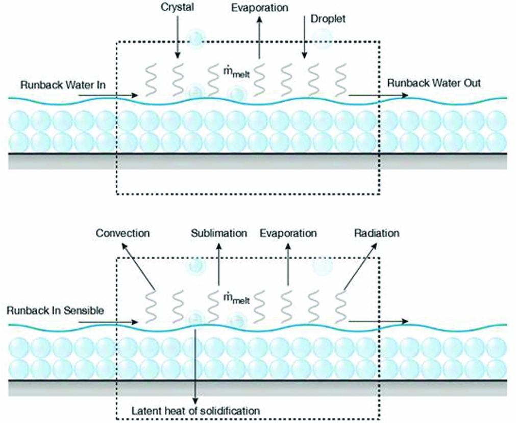
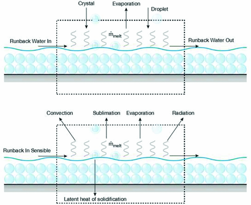
Thus, the melting ratio is an additional unknown and can be predicted by solving the energy balance equation. Energy and mass terms which are included in the control volume are depicted in Fig. 3.
Mass and energy terms in the balance equations.
The energy terms that contribute to the energy balance are as follows:
 $$\begin{equation}
\lambda _{h,w} = r_l \rho _l \beta _l V_\infty C_{pw}\left[T_f-T_l\right]+\dot{m}_{in}C_{pw}\left[T_f-T_{in}\right],\\
\end{equation}$$
 $$\begin{equation}
\lambda _{h,i} = r_c \rho _c \beta _c V_\infty (1-\eta _{melt})C_{pi}\left[T_f-T_c\right]+r_c \rho _c \beta _c V_\infty \eta _{melt}C_{pw}\left[T_f-T_c\right], \\
\end{equation}$$
 $$\begin{equation}
\lambda _{in} = r_l \beta _l V_\infty \frac{V_{imp,l}^2}{2}+r_c \beta _c V_\infty \frac{V_{imp,c}^2}{2}, \\
\end{equation}$$
 $$\begin{equation}
\lambda _{out} = h_c\left[T_{rec}-T_f\right]+\dot{m}_{ev}L_{ev}
\end{equation}$$
The first term in previous equations, λ h, w , refers to the heat transfer due to impinging droplets and runback water in. Heat transfer due to impinging solid and liquid parts of ice crystals are calculated by the second relation, λ h, i . On the other hand, λ in refers to the total kinetic energy of the upcoming particles and λ out shows heat transfer due to convection and evaporation. Inclusion of the heat loss by melting part of the incoming ice crystals causes an imbalance in the energy equation and this must be compensated by additional freezing. Thus, at melting temperature, the net energy before computing the melting ratio can be calculated as follows:
 $$\begin{equation}
\lambda _{net} = \lambda _{in}-\lambda _{out}-\lambda _{h,w}-\lambda _{h,i} \\
\end{equation}$$
 $$\begin{equation}
\alpha _{melt} = \frac{\lambda _{net}}{r_c \rho _c \beta _c V_\infty L_f}
\end{equation}$$
Three different scenarios are possible after calculating the net energy terms:
-
• When λ net > 0 and α melt < 1, some energy is available in the control volume and it will melt some part of the ice crystals. Surface temperature of the water layer will be equal to the melting temperature.
-
• When λ net > 0 and α melt > 1, some energy is available in the control volume and all ice crystals will melt. Remaining energy will increase the temperature of the water layer and the surface temperature of the water layer will be greater than the melting temperature.
-
• When λ net < 0, all upcoming ice crystals will stay as solid, even after impact. The surface temperature of the water layer will be less than the melting temperature.
Next, it is assumed that the temperature profile in the ice layer is linear:
 $$\begin{eqnarray}
\frac{\partial ^2 T}{\partial y^2}=0
\end{eqnarray}$$
Integrating twice T(y, t) can be obtained:
 $$\begin{eqnarray}
T(y,t)=a_3 y+a_4
\end{eqnarray}$$
Employing the condition defined in Equation (18) yields:
 $$\begin{eqnarray}
a_4=T_{subs}
\end{eqnarray}$$
Thus, at y = B:
 $$\begin{eqnarray}
T_f=a_3B+T_{subs}
\end{eqnarray}$$
Assume that the temperature profile in the water layer is linear as well:
 $$\begin{eqnarray}
\frac{\partial ^2 \theta }{\partial y^2}=0
\end{eqnarray}$$
Integrating twice:
 $$\begin{eqnarray}
\theta (y,t)=a_5 y+a_6
\end{eqnarray}$$
Employing Condition 14 yields:
 $$\begin{eqnarray}
T_f=a_5B+a_6
\end{eqnarray}$$
In Equation (68), the calculation of a 5 is not necessary when the temperature of the water layer surface is equal to the melting temperature, which corresponds to the 0 < α melt < 1 case. However, for other cases, the condition defined in Equation (18) needs to be imposed:
 $$\begin{eqnarray}
-k_wa_5=(Q_{con}+Q_{ev}+Q_{cl}+Q_{ccs}+Q_{ccl})-(Q_{aero}+Q_{kl}+Q_{kc}+Q_{in})
\end{eqnarray}$$
Substituting Q con , Q ev , Q cl , Q ccs , Q ccl and Q in from Equations (33) to (40):
 $$\begin{eqnarray}
a_5=\frac{-(a+b+c+e)\theta (B+h,t)+aT_a+bT_l+cT_c+eT_f+d}{k_w},
\end{eqnarray}$$
where
 $$\begin{equation}
a = h_c, \\
\end{equation}$$
 $$\begin{equation}
b = r_l \rho _l \beta _l V_\infty C_{pw}, \\
\end{equation}$$
 $$\begin{equation}
c = r_c \rho _c \beta _c V_\infty \left(\left(1-\eta _{melt}\right)C_{pi}+\eta _{melt}C_{pw}\right), \\
\end{equation}$$
 $$\begin{equation}
d = Q_{aero}+Q_{kl}+Q_{kc}+Q_{in}, \\
\end{equation}$$
 $$\begin{equation}
e = \dot{m}_{in}C_{pw}
\end{equation}$$
Evaluating Equation (67) at y = B + h, substituting a 5 from Equation (70):
 $$\begin{eqnarray}
\theta (B+h,t)=\frac{k_wT_f+(aT_a+bT_l+cT_c+eT_f+d)h}{k_w+(a+b+c+e)h}
\end{eqnarray}$$
For the calculation of Q ev in Equation (33), vapour pressure needs to be calculated. This is a function of θ(B + h, t). Therefore, θ(B + h, t) needs to be calculated through an iterative process until convergence in Q ev is reached.
Substituting θ(B + h, t) from Equation (76) back into Equation (67):
 $$\begin{equation}
a_5=\frac{a(T_a-T_f)+b(T_l-T_f)+c(T_c-T_f)+d+e(T_in-T_f)+f(T_a-T_f)}{k_w+(a+b+c+e)h}
\end{equation}$$
Therefore, Equation (67) becomes:
 $$\begin{eqnarray}
\theta (y,t)=a_5 y+T_f
\end{eqnarray}$$
Integrating Equation (16) yields:
 $$\begin{equation}
h=\frac{r_l \rho _l \beta _l V_\infty + \eta _{melt} r_c \rho _c \beta _c V_\infty + \alpha _{melt} r_c \rho _c \beta _c V_\infty + \dot{m}_{in}- \dot{m}_{ev}}{\rho _w}(t-t_g)-\frac{\rho _g}{\rho _w}(B_l-B_g)
\end{equation}$$
This integration involves B g and t g constants which are the ice thickness and time at which water first appears in glaze ice. Substituting Equation (55) and (78) into Equation (17) yields:
 $$\begin{eqnarray}
\rho _gL_f \frac{\partial B_l}{\partial t}&=&k_i\frac{T_f-T_{subs}}{B_l}-k_wa_5
\end{eqnarray}$$
Here, a 5 can be calculated from Equation (77) and h from Equation (79). In order to find B g (hence t g ), substitute ∂B l /∂t from Equation (42) into Equation (80). However, only the ice thickness due to liquid water coming from droplets or the liquid part of partially melted ice crystals is taken into account:
 $$\begin{eqnarray}
L_f\left(r_l \rho _l \beta _l V_\infty + \eta _{melt} r_c \rho _c \beta _c V_\infty + \dot{m}_{in}- \dot{m}_{sub}\right)=k_i\frac{T_f-T_{subs}}{B_g}-k_wa_5
\end{eqnarray}$$
Rearranging:
 $$\begin{eqnarray}
B_g=\frac{K_i(T_f-T_{subs})}{(r_l \rho _l \beta _l V_\infty + \eta _{melt} r_c \rho _c \beta _c V_\infty + \dot{m}_{in}- \dot{m}_{sub})L_f+k_wa_5}
\end{eqnarray}$$
Note, a 5 has to be calculated for h = 0 here because at B = B g , h = 0:
 $$\begin{equation}
a_5=\frac{a(T_a-T_f)+b(T_l-T_f)+c(T_c-T_f)+d}{k_w}
\end{equation}$$
The time at which glaze ice first appears is found from Equation (42):
 $$\begin{eqnarray}
t_g&=&\frac{\rho _r}{r_l \rho _l \beta _l V_\infty + r_c \rho _c \beta _c V_\infty + \dot{m}_{in}- \dot{m}_{sub}}B_g
\end{eqnarray}$$
When we collect all unfrozen water in one term, by rewriting
 $\dot{m}_{i}$
:
 $$\begin{eqnarray}
\dot{m}_{w}=\frac{\rho _wh}{t-t_g}
\end{eqnarray}$$
 $$\begin{eqnarray}
\dot{m}_{i}=\rho _g \frac{\partial B_l}{\partial t}
\end{eqnarray}$$
As discussed in the erosion model part, water and ice erosion rates can be related with the total erosion rates as follows:
 $$\begin{eqnarray}
\dot{m}_{er,i}&=&\dot{m}_{er}\frac{\dot{m}_{i}}{\dot{m}_{i}+\dot{m}_{w}}
\end{eqnarray}$$
 $$\begin{eqnarray}
\dot{m}_{er,w}&=&\dot{m}_{er}\frac{\dot{m}_{w}}{\dot{m}_{i}+\dot{m}_{w}}
\end{eqnarray}$$
Water and ice mass accumulation rates can be updated after calculating the erosion rates:
 $$\begin{eqnarray}
\dot{m}_{i,upd}&=&\dot{m}_{i}-\dot{m}_{er,i}
\end{eqnarray}$$
 $$\begin{eqnarray}
\dot{m}_{w,upd}&=&\dot{m}_{w}-\dot{m}_{er,w}
\end{eqnarray}$$
Moreover, Trontin suggested that some of the accreted water does not run downstream and is trapped inside the accumulated ice layer(Reference Trontin, Blanchard and Villedieu28).
 $$\begin{eqnarray}
\dot{m}_{out}&=&2\zeta \dot{m}_{w,upd}
\end{eqnarray}$$
 $$\begin{eqnarray}
\zeta &=&\frac{\psi _l+\eta _{melt}\epsilon _s\psi _c}{\psi _l+\epsilon _s\psi _c}
\end{eqnarray}$$
The above relation is applicable only when ζ ⩽ 0.5. Otherwise, all the accreted water is assumed to run downstream.
3.0 RESULTS
For validation studies, it is possible to find a wealth of experimental results in the literature to be used for ice accretion studies. However, most of these ice accretion experiments are done in liquid phase cloud conditions only. In other words, a very limited number of them can be applicable to mixed phase icing cases including ice crystals. In this study, the Cox and Technical University of Braunschweig (TUBS) experimental test conditions and results for mixed phase are used for erosion and impingement models calibration purposes. It should be noted that all reference values, all power terms and erosion efficiency terms in Equation (11) and K l in the impingement model are the free parameters for calibration.
3.1 Validation by Using Cox Icing Wind-Tunnel Experimental Results
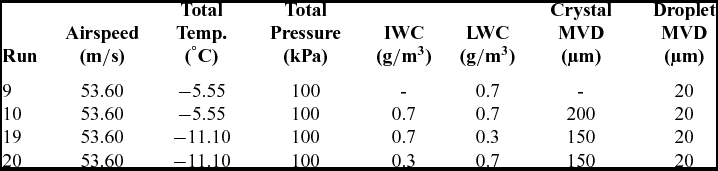
Al-Khalil et al(Reference Al-Khalil, Irabi and Miller1) performed mixed phase ice accretion experiments by using NACA 0012 aerofoil having a 0.9144 m chord length. The test section in the icing wind tunnel has a height of 1.83 m and a width of 2.74 m. Ice accretion was recorded with a high-speed camera system and photos of the corresponding ice shapes are included in the manuscript. The authors did not give any information about the error or standard deviation of the tests. Moreover, it is assumed that the included ice shapes belong to the mid-span of the test model. The aim of this comparison is to validate mixed phase ice accretion models and the erosion model implemented in the current computational tool. For validation purposes, two rime ice and two glaze ice test cases are selected. Experimental data is digitised from the given ice shapes in the manuscript(Reference Al-Khalil, Irabi and Miller1). Flow and icing parameters of the selected test cases are given in Table 1. The aerofoil is placed in the middle of the test section and mounted horizontally and the angle-of-attack is 0°.
Cox icing experiments run conditions

A mono-disperse distribution of the injected ice particles and water droplets is assumed. The MVD for ice crystals is 150 µm for runs 19 and 20 (snow gun) and around 200 µm for run 10. For the water droplets, the MVD is 20 µm. For all computations, the heat exchange between the particles and the surrounding air is neglected. Thus, mass loss of particles due to evaporation and sublimation is also neglected. Total experiment duration is 600 seconds for all run conditions.
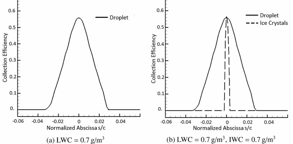
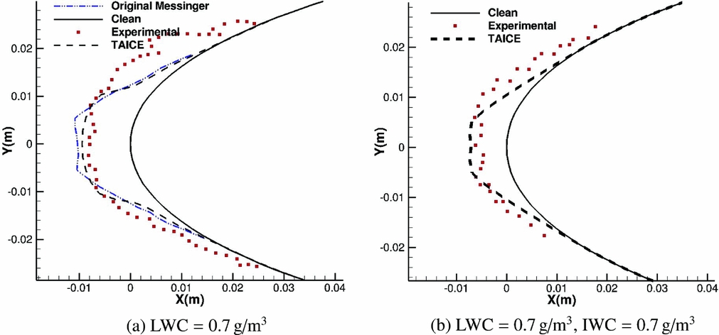
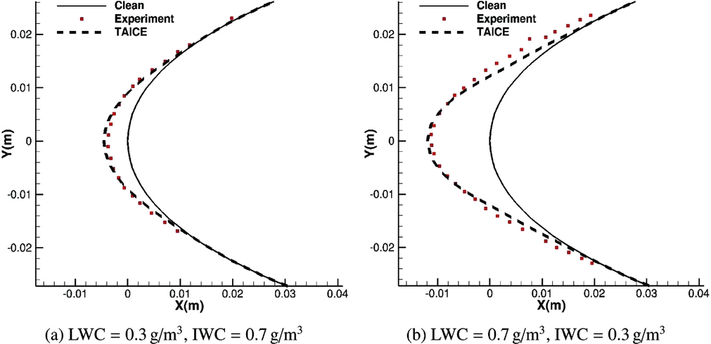
Collection efficiencies of runs 9 and 10 are depicted in Fig. 4 and corresponding ice shape comparisons with experimental shapes are shown in Fig. 5. These two cases correspond to glaze ice conditions due to high temperature, which is also made evident by the ice shapes depicted in Fig. 5. On the other hand, runs 19 and 20 correspond to rime ice conditions due to low temperatures which is evidenced by the ice shapes in Fig. 7.
Collection efficiency curves of liquid and solid cloud particles for (a) run 9 pure droplet case (b) run 10 mixed phase case.

Ice shape comparisons for (a) run 9 pure droplet case and (b) run 10 mixed phase case.
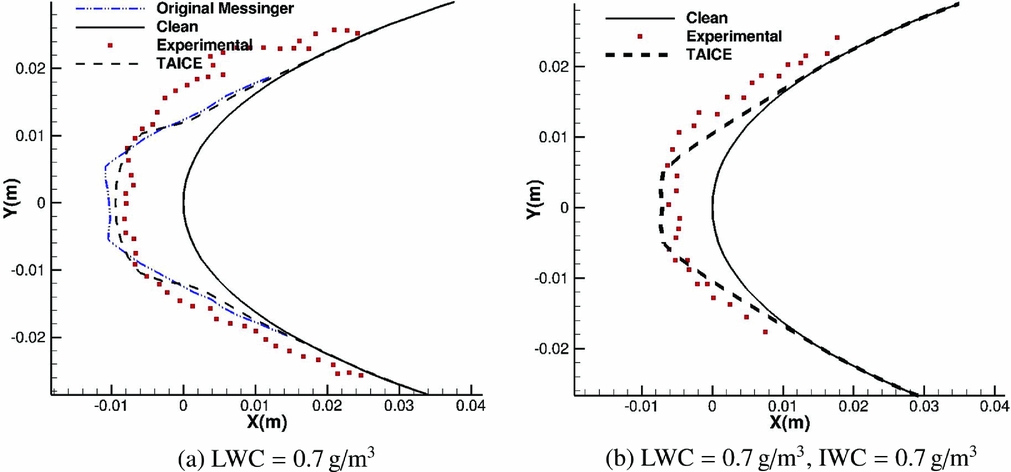
For the pure droplet case, Original Messinger Model predictions are also given in addition to the present model. By calibration, it is possible to obtain similar results with this method as well. Better predictions of the Extended Messinger Model has been validated for ice accretion due to water droplets only before(Reference Myers22,Reference Özgen and Canıbek24,Reference Özgen and Canıbek25) . Since rime to glaze ice transition is not modelled in the Original Messinger Model, the authors envisaged that accuracy of the predictions would be less and calibration would be difficult if more experimental results are used especially in glaze ice conditions with the Original Messinger Model.
When collection efficiencies of liquid and solid cloud particles are compared, quite different curves are obtained, mainly due to the bouncing solid particles as they are shown in Fig. 4. In run 9, only droplet particles were used as depicted in Fig. 7. Formation of horns indicates glaze ice accretion where excess water moves to the neighbouring cells as runback water. Moreover, Original Messinger Model results are given in this run condition as well. This comparison demonstrates marginal improvement in ice accretion prediction capability for the Extended Messinger Model.
Erosion effects on accreted ice are more significant than in rime ice conditions in these mixed phase tests. In run 10, in which frozen ice crystals are added, the accreted ice decreases significantly. A slight reduction in accreted ice around the stagnation area can be seen in the comparisons. Erosion phenomena might be the main reason for this reduction.
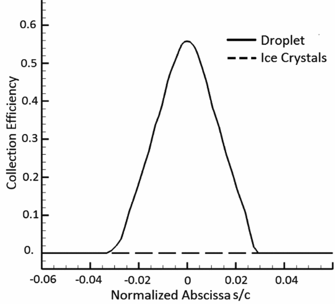
In Figs 6 and 7, it is clearly seen that for run 19 and run 20, ice accretion occurs only due to supercooled water droplets present in the cloud because the collection efficiency of the ice crystals is zero. Since liquid water does not accumulate above the ice layer, ice crystals do not stick to the surface and, hence, do not contribute to ice accretion. The only observable effect of the ice crystals is the erosion of the accreted ice near the impingement limits.
Collection efficiency curves of liquid and solid cloud particles for run 19 and run 20.

Ice shape comparisons for (a) run 19 and (b) run 20.

3.2 Comparisons by Using TUBS Experimental Data
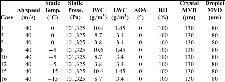
Icing experiments have been performed in the TUBS icing wind-tunnel facility. NACA 0012 aerofoil having 0.5 m chord has been used in these tests. Selected icing conditions for the validation analyses are given in Table 2 (Reference Bansmer and Baumert3,Reference Baumert, Trontine, Bansmer and Villedieu5) . Tests have been performed at three different temperatures, and at each temperature, LWC and IWC values are varied. Droplet clouds have been generated by a spray bar within 1.3 to 5 g/m 3. On the other hand, ice crystals have a wider range and IWC of the injected crystals have been increased up to 13.6 g/m 3. The accretion time is 2 minutes for all runs. Further details about the experiments and corresponding data can be found in the study of Baumert et al(Reference Baumert, Bansmer, Sattler, Pervier and Esposito4,Reference Baumert, Trontine, Bansmer and Villedieu5) and Bansmer et al(Reference Bansmer and Baumert3).
Experimental conditions in TUBS experiments

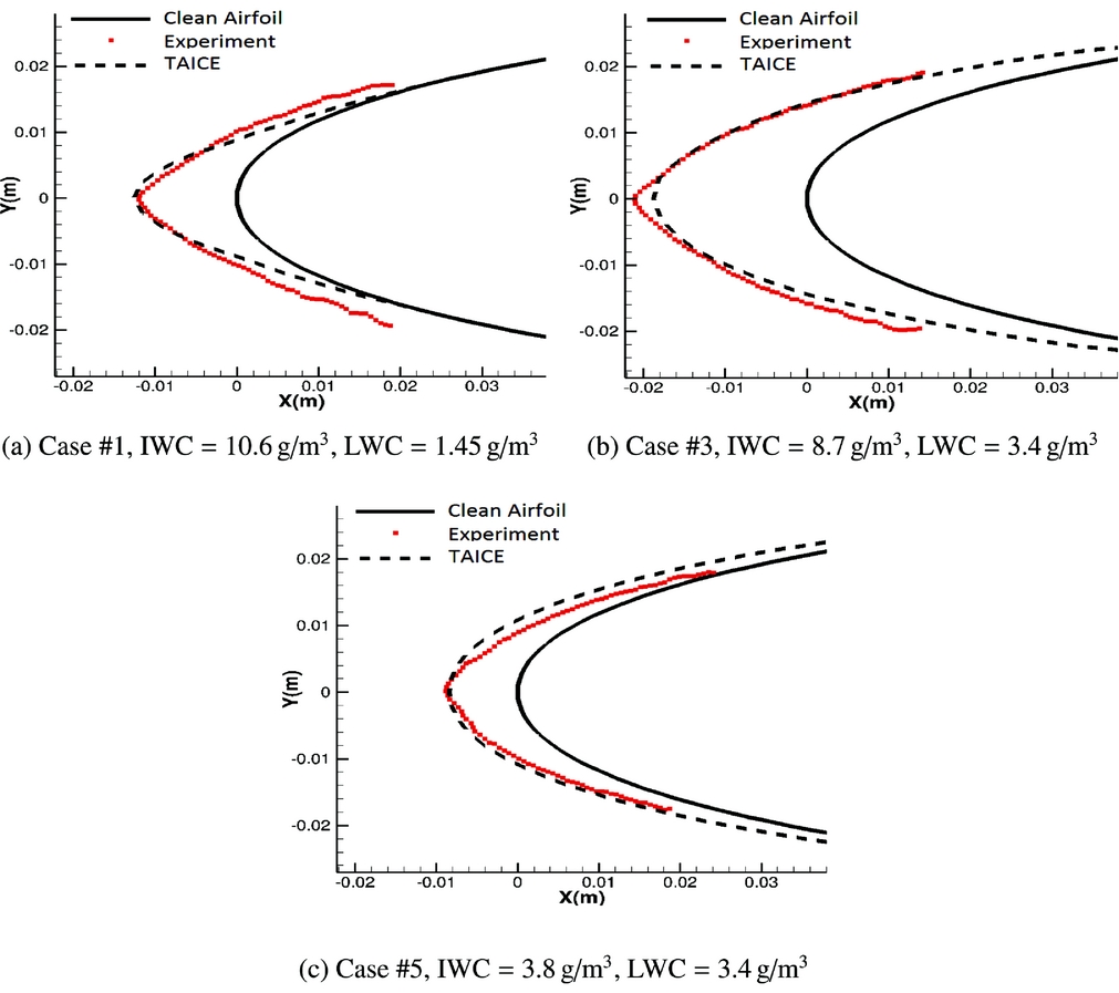
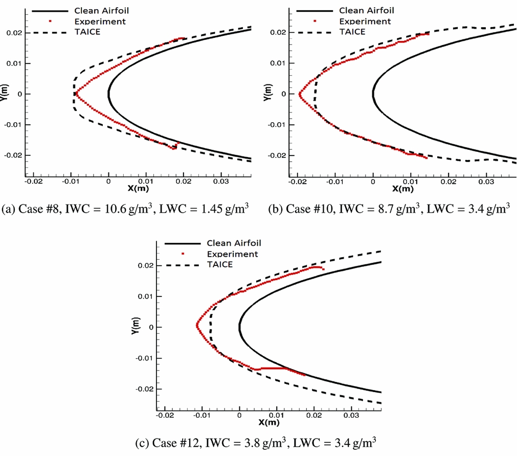
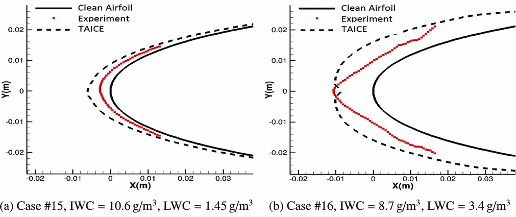
Calculated and experimental ice shapes on the NACA 0012 aerofoil are depicted in Figs 8–10. Differing from the COX experiments, IWC and LWC values are much higher here. Thus, erosion and impingement models require further calibration.
Ice shape comparisons at T s = 0 °C.

Ice shape comparisons at T s = −5 °C.

Ice shape comparisons at T s = −15 °C.

The following figures indicate that increasing the droplet ratio first causes more ice crystals to stick to the surface. However, further increase in the droplet ratio does not cause additional increase in the thickness of the accreted ice. On the contrary, reduction in the accumulated ice has been noted due to the erosion effect in these experimental tests. Analysis results seem consistent with the experimental data for all compared conditions. However, a few points should be emphasised here. First of all, accreted ice in the experiments have triangular shapes and sharp edges. On the other hand, ice shapes obtained with TAICE are more smooth. Moreover, at −15 ℃, TAICE overestimates the ice shapes, which indicates that the erosion effect is more than predicted at this temperature.
3.3 Assessment of Parameters Affecting Ice Shapes
This section gives information about the analysis parameters which affect the accreted ice shapes. Analyses are performed by varying each parameter and results are compared with glaze icing experimental case #10 in Table 1 (Reference Al-Khalil, Irabi and Miller1).
3.3.1 Number of time steps
It is known that accreted ice on a body has influence on the flowfield. Single step analyses mostly lead to wrong ice shapes due to this reason. Moreover, too much increase in the number of time steps is also not preferred due to possible numerical errors such as round-off. Thus, multi-step analyses should be performed in order to increase the accuracy of the predictions. Determining the number of time steps for each ice accretion analysis requires a preliminary assessment as stated in the LEWICE manual(Reference Wright20). A relation similar to the recommended one in the LEWICE manual is used in this study. It should be noted that in order to use this relation for mixed phase icing cases, IWC is also included in addition to the LWC. However, this relation is applicable only to glaze ice conditions. Since in rime ice conditions, the effect of ice crystals on accreted ice shapes can be negligible in most cases including IWC, in this relation, it may lead to wrong time-step numbers.
 $$\begin{eqnarray}
N=\frac{(LWC+IWC)(V)(Time)}{(chord)(\rho )(0.01)}
\end{eqnarray}$$
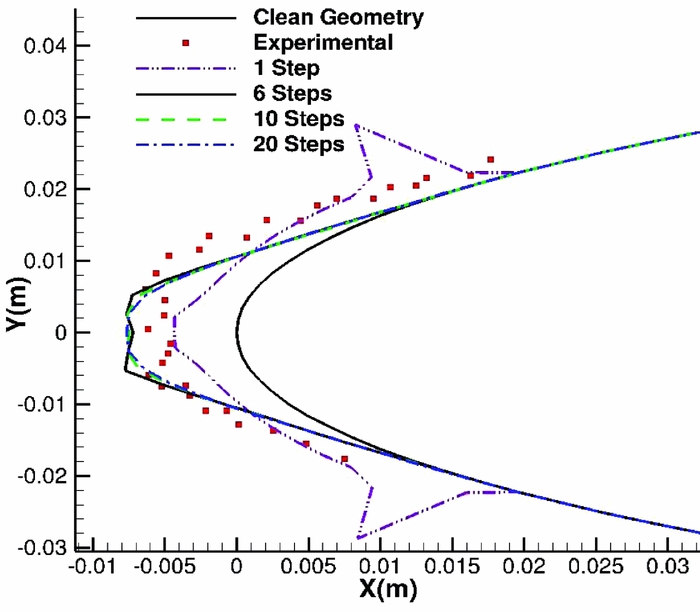
Analyses are performed for 1, 6, 10 and 20 multi-steps and corresponding comparisons are depicted in Fig. 11. Required number of time steps is six according to Equation (93) when the nearest integer number is chosen. As expected, a further increase in time-step number does not increase the accuracy of the predictions. Moreover, since the number of steps directly influences the analyses duration, it causes further increase in the cost of the analyses. On the other hand, results obtained with lower step numbers are unacceptable due to low accuracy.
Ice shape comparisons for varying time-step numbers from 1 to 20.

3.3.2 Number of panels
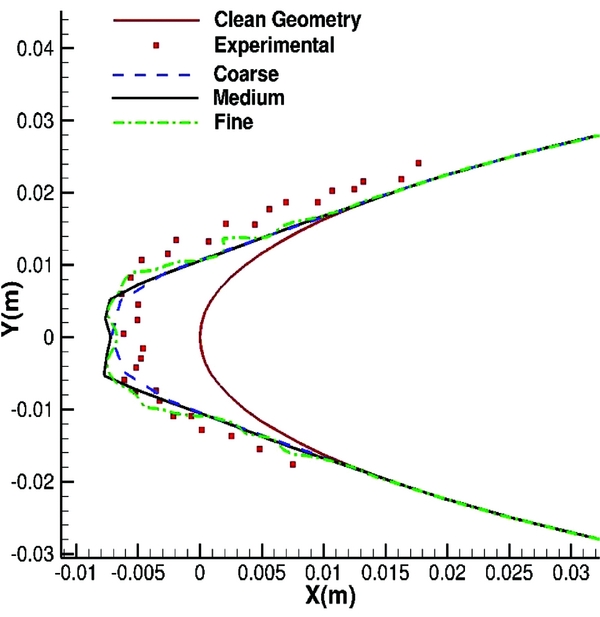
Number of panels and boundary-layer grids have direct influence on accreted ice on the surface. One reason is that they affect flowfield variables and heat transfer coefficients. Another reason is that the ice thicknesses are calculated for these points. A comparison is shown in Fig. 12 for three different panel numbers and corresponding computational times are given in Table 3.
Ice shape comparisons for varying panel numbers.

Number of panels and boundary-layer grids

As it is depicted in Fig. 12, varying numbers of panels change the accreted ice on the surface. The accuracy of the coarsest one is good, but capturing shape and amount of calculated complicated ice shapes will be difficult due to less number of panels. Predictions of the fine one is also acceptable, but it increases the computational time as shown in Table 3. Thus, having nearly the same accuracy, the medium one is chosen as the optimum number of panels and is used in the calibration studies.
4.0 CONCLUSION
A mathematical model which was initially developed by Myers(Reference Myers22) has been further extended in this study by including solid ice particles in the computations. In Myers approach, temperature variations along both ice and water layers are modelled. With a fixed and known temperature at the substrate, initially, rime ice grows until the surface temperature of the ice layer reaches the freezing temperature. At this time, substrate becomes totally insulated and this yields both ice and water accretion on the surface. In addition to separately modelled ice and water layers, another advantage of using this approach is that it provides an exact formula for the ice thickness in which glaze ice is first observed. However, up to now, this model has not been extended further for mixed cloud icing conditions to the authors’ best knowledge. This was a motivating factor for the authors to focus on this problem. On the other hand, in the Original Messinger Model, it is not possible to model the rime to glaze ice transition and this may lead to problems while taking into account the effect of ice crystals in glaze ice accretion.
The mentioned extension of the Extended Messinger Model is not sufficient for accurate prediction alone. To improve accuracy, particle trajectory and impingement calculations in TAICE have been modified as well. Initially, TAICE, which is an in-house developed ice accretion prediction tool, was applicable to icing conditions including only water droplets. Heat transfer, phase change, drag force coefficient, impingement and erosion models have been implemented in order to utilise this tool for mixed phase icing conditions thanks to the HAIC project.
Calibrated erosion and impingement models are used in the analyses with two different sets of experimental data and good predictions for the ice shapes have been noted for both cases. K l in the impingement model, erosion efficiency, reference velocity and reference surface temperature in the erosion model are the free parameters for calibration study. The same values are used for both of the experimental tests, and corresponding parameters are given in impingement and erosion model parts. However, the number of validation cases used is not enough to reach a final decision on the validity of the developed computational tool. Generally, rime ice predictions seem to agree better with experiment compared to the glaze ice predictions. The accuracy of the numerical results decreases when the influence of ice crystals on the accreted ice shape increases. Moreover, it should be noted that due to the lack of experimental mixed phase icing data, it is not possible to show the superiority of the Extended Messinger Model over the Original Messinger Model by making ice shape comparisons. However, for pure droplet cases, ice accretion prediction success of the Extended Messinger Model has been shown previously. Thus, in this study, a better model is used for mixed phase ice accretion prediction. Future work will focus on further validations of the tool by using new data and models developed using mixed phase icing experiments.
APPENDIX
A.0 TRAJECTORY MODELS
A.1 LIQUID DROPLETS
Drag force coefficient of the droplets is calculated with the following model as Gent et al suggested(Reference Gent, Dart and Cansdale13).
 $$\begin{equation}
C_D=\left(\frac{1}{24}\right) \left\lbrace \begin{array}{@{}l@{\quad }l@{}}1+0.197Re^{0.63}+2.6x10^{-4}Re_p^{1.38} ,& \text{if } {\it Re} \le {\it 3500} \\
(1.699x10^{-5})Re_p^{1.92} ,& \text{if } {\it Re} > {\it 3500} \\
\end{array}\right.
\end{equation}$$
 $$\begin{eqnarray}
Re_p=\frac{\rho _ad_pV_{rel}}{\mu }
\end{eqnarray}$$
 $$\begin{eqnarray}
V_{rel}=V-V_{\infty },
\end{eqnarray}$$
where V rel is the relative velocity of the particle with respect to the air flow and μ is the dynamic viscosity. Sutherland viscosity law is used for calculating this parameter.
A.2 ICE CRYSTALS
Before discussing the drag coefficient, heat transfer and phase change models in detail, geometrical properties of ice crystals are first given.
A.2.1 Ice crystal particle geometric properties
Since ice crystals are not exactly spherical, an equivalent volumetric diameter d p should be used for such particles which can be calculated as follows:
 $$\begin{eqnarray}
d_p= 3\sqrt{\frac{6v_p}{\pi }},
\end{eqnarray}$$
where v p is the volume of the ice crystal particle. Moreover, sphericity, which is a measure of how close an object is to a sphere should be introduced.
 $$\begin{eqnarray}
\phi =\frac{\pi d_p^{2}}{A_s}
\end{eqnarray}$$
In the above relation, A s denotes the surface area of the particle. Another parameter which is related with the orientation of the particle with respect to air flow, is crosswise sphericity and can be specified as follows:
 $$\begin{eqnarray}
\phi _\perp =\frac{\pi r_p^{2}}{A_\perp },
\end{eqnarray}$$
where A ⊥ is the projected area of the particle with respect to the flow.
Calculations of sphericity and crosswise sphericity are generally given in terms of two other important parameters, which are aspect ratio E and eccentricity e. They can be specified as follows:
 $$\begin{eqnarray}
E&=&\frac{d_1}{d_2}
\end{eqnarray}$$
 $$\begin{eqnarray}
e&=&\sqrt{1-\min \left[\frac{d_1}{d_2},\frac{d_2}{d_1}\right]^2},
\end{eqnarray}$$
where d 1 and d 2 are diameters of the particle, parallel and perpendicular to the revolution axis, respectively. In these equations, aspect ratio is used for classification of the spheroid geometry as oblate (E < 1) or prolate (E > 1).
Thus, sphericity for oblate particles is:
 $$\begin{eqnarray}
\phi &=&\frac{4E^{2/3}}{2+E^2e^{-1}\ln \bigg ((1+e)(1-e)^{-1}\bigg )}
\end{eqnarray}$$
and for prolate particles:
 $$\begin{eqnarray}
\phi &=&\frac{2E^{2/3}}{1+Ee^{-1}\arcsin {e}}
\end{eqnarray}$$
During the trajectory of the particle, it is assumed that once it reaches to a stable orientation, it stays in that orientation. Thus, crosswise sphericity can be reduced to the following relations for oblate and prolate particles, respectively:
 $$\begin{eqnarray}
\phi _\perp &=&E^{{2}/{3}}
\end{eqnarray}$$
 $$\begin{eqnarray}
\phi _\perp &=&E^{{-1}/{3}}
\end{eqnarray}$$
A2.2 Drag force coefficient models
Since ice crystal particles may not be spherical, lift force can appear depending on the orientation of the particle. Moreover, a particle may rotate and change its orientation during the trajectory. However, in order to reduce the computational cost of the analyses, it is assumed that a particle travels with fixed orientation without rotating. In the literature, it is possible to find several drag force coefficient models, but only some of them are applicable to non-spherical particles. In this study, only most widely used models are discussed.
Haider and Levenspiel suggest a model in terms of ϕ and Rep and it is supposed to be valid for the particles having crosswise sphericity around 1(Reference Haider and Levenspiel14):
 $$\begin{equation}
C_d = \left[\frac{24}{Re_p}\left[1+a\left(Re_p^{b}\right)\right]\right]+\frac{cRe_p}{Re_p+d} \\
\end{equation}$$
 $$\begin{equation}
Re_p = \frac{\rho _ad_pV_{rel}}{\mu },
\end{equation}$$
where ρ a is air density and V rel is the relative velocity of the particle, and μ is the dynamic viscosity.
The following terms should be defined:
 $$\begin{equation}
a = exp\left(2.4486 \phi ^{2} -6.5481 \phi +2.3288\right)\\
\end{equation}$$
 $$\begin{equation}
b = 0.5565 \phi + 0.0964\\
\end{equation}$$
 $$\begin{equation}
c = exp\left(-10.2599 \phi ^{3} +18.4222 \phi ^{2} -13.8944 \phi +4.905\right)\\
\end{equation}$$
 $$\begin{equation}
d = exp\left(15.8855 \phi ^{3} -20.7322 \phi ^{2} +12.2584 \phi + 1.4681\right)
\end{equation}$$
In the previous relation, crosswise sphericity ϕ⊥ is not included. Thus, Ganser(Reference Ganser12) has suggested another model which also takes crosswise sphericity into consideration.
 $$\begin{equation}
C_d = \left[\bigg [\left(24/Re^*_p\right)\left(1+0.1118Re^{*0.6567}_p\right)\bigg ]+\frac{0.4305 Re^*_p}{Re^*_p+3305}\right]C_{d,ct}\\
\end{equation}$$
 $$\begin{equation}
Re^*_p = \frac{Re_p}{\frac{2}{3}\phi ^{-1/2}+\frac{1}{3}\phi _\perp ^{-1/2}}C_{d,ct}\\
\end{equation}$$
 $$\begin{equation}
\log {C_{d,ct}} = 1.8148\left(-\log \phi \right)^{0.5743}
\end{equation}$$
Moreover, an additional drag model including ϕ⊥ is suggested by Hölzer and Sommerfeld(Reference Hölzer and Sommerfeld19):
 $$\begin{equation}
C_d=\frac{8}{Re_p}\frac{1}{\phi _\perp ^{1/2}}+\frac{16}{Re_p}\frac{1}{\phi ^{1/2}}+\frac{3}{Re_p^{1/2}}\frac{1}{\phi ^{3/4}}
\end{equation}$$
A.2.3 Heat transfer and phase change models
Temperatures of the particles may change due to heat transfer between particle and surrounding air along the trajectory of the ice crystals. Moreover, if their temperature increases up to the melting point, they may even change phase before impinging to the surface. Since this may lead to change in accumulated ice on the surface, it should be taken into consideration. In simplest form, the Nusselt number can be calculated with the following relation(Reference Villedieu, Trontin and Chauvin30):
 $$\begin{equation}
Nu=\frac{h_td_p}{k_a}
\end{equation}$$
Here, h t refers to the heat transfer coefficient and k a refers to air heat conductivity. Moreover, general form of the heat transfer equation in the absence of phase change relations:
 $$\begin{equation}
m_pC_p\frac{dT_{p,m}}{dt}=\pi d_p\frac{Nu}{\phi }k_a(T_a-T_{p,s}),
\end{equation}$$
where m p refers to particle mass, C p is specific heat at constant pressure, T a is air temperature, T p, m is the mean particle temperature and T p, s is the particle surface temperature.
On the other hand, the Nusselt number formulation can be defined in terms of ϕ, ϕ⊥, Re p and Pr:
 $$\begin{equation}
Nu=1.76+0.55\phi Re^{\frac{1}{3}}_p Pr^{\frac{1}{3}} \phi _\perp ^{0.0075}+0.014 Re^{\frac{2}{3}}_p Pr^{\frac{1}{3}}\left(\frac{\phi }{\phi _\perp }\right)^{7.2}
\end{equation}$$
Theoretically, the above relation can be applied to all particles. However, when the aspect ratio of the particle is less than 0.8, this relation produces unrealistic results. Thus, Villedue et al(Reference Trontin, Blanchard and Villedieu28) suggested an extension of the Frössling correlation that can be applied to all particles.
 $$\begin{equation}
Nu=2\sqrt{\phi }+0.55Pr^{\frac{1}{3}}\phi ^{0.25}Re_p^{0.5}
\end{equation}$$
Phase change equations can be divided into three parts according to Mason’s study(Reference Mason, Strapp and Chow21). Before proceeding to the relations, assumptions should be discussed.
-
• The ice core temperature is constant during melting phase and equal to T f .
-
• The melting process begins when the ice core temperature of the particle reaches T f .
-
• The ice core is spherical and concentric.
-
• Heat transfer between the ice core and surrounding liquid film is purely conductive.
-
• The ice crystals do not shed their liquid film during the melting phase.
Starting from Mason’s study, many improvements have been performed on this model. Rasmussen et al take eccentric location of the ice core and influence of an internal circulation into consideration(Reference Rasmussen, Levizzani and Pruppacher26). Furthermore, Villedue et al included the effect of non-sphericity and noted the decrease in the melting time(Reference Villedieu, Trontin and Chauvin30).
When T p < T f , the ice crystal temperature increases up to the melting temperature. Particle mass may change by sublimation in this step and can be calculated as follows:
 $$\begin{equation}
\frac{dm_p}{dt}=-\pi d_p\frac{Sh}{\phi }\rho _aD_{v,a}(y_{v,s}-y_{a,s})
\end{equation}$$
In the above relation, D v, a is vapour diffusivity of air and Sh is the Sherwood number and can be calculated with the Chilton-Colburn analogy. Again, in the same relation, y v, s and y a, s are vapour mass fractions at the particle surface and at free stream, respectively.
 $$\begin{equation}
D_{v,a} = 0.0000226\left(\frac{T_p}{273.15}\right)^{1.81}\left(\frac{10000}{P_a}\right)\\
\end{equation}$$
 $$\begin{equation}
Sh = 2\sqrt{\phi }+0.55Sc^{\frac{1}{3}}\phi ^{0.25}Re_p^{0.5}\\
\end{equation}$$
 $$\begin{equation}
y_{v,s} = \frac{M_v}{M_m}\frac{P_{sat}T_{p,s}}{P_a}\\
\end{equation}$$
 $$\begin{equation}
y_{v,a} = \frac{M_v}{M_m}\frac{P_{sat}T_a(RH)}{P_a},
\end{equation}$$
 $$\begin{equation}
Sc=\frac{\nu }{D_{v,a}}
\end{equation}$$
Moreover, saturated pressure relations (in Pa) over ice and over water are:
 $$\begin{equation}
P_{sat,w}(T)=exp\left(-6024.53 T^{-1}+29.32+1.06\times 10^{-2} T-1.32\times 10^{-5} T^{2}-0.49 \ln T\right)
\end{equation}$$
 $$\begin{equation}
P_{sat,i}(T)=exp\left(-6093.94 T^{-1}+24.10+2.71\times 10^{-2} T+1.67\times 10^{-5} T^{2}-2.43 \ln T\right)
\end{equation}$$
Thus, by assuming constant particle density ρ p , the final heat transfer equation becomes:
 $$\begin{equation}
\pi \rho _p\frac{dp^{3}}{6}C_i\frac{dT_p}{dt}=\pi d_p\frac{Nu}{\phi }k_a(T_a-T_p)-\dot{m}_{sub}(L_f+L_v)
\end{equation}$$
In the above relation, L f and L v are the latent heat of fusion and latent heat of evaporation at the particle temperature.
When T p = T f , the particle starts to melt at a constant temperature and is surrounded with concentric water film. Moreover, the particle mass may reduce due to evaporation and this step continues until the ice particle is completely melted. At the end of this step, the particle becomes completely spherical. Thus, the heat transfer relation is:
 $$\begin{equation}
\pi d_p \frac{Nu}{\phi }k_a(T_a-T_f)=\dot{m}_{ev}L_v+\dot{m}_{f}L_f,
\end{equation}$$
where
 $\dot{m}_{ev}$
is the evaporation rate and can be calculated with the following relation:
 $$\begin{equation}
\dot{m}_{ev}=-\frac{dm_p}{dt}=\pi d_p \frac{Sh}{\phi }\rho _aD_{v,a}(y_{v,s}-y_{a,s})
\end{equation}$$
Reduction in the mass of ice may be directly related with the melting rate as follows:
 $$\begin{equation}
m_{p,i}=\pi \rho _{p,i}\frac{d_{p,i}^{3}}{6}
\end{equation}$$
 $$\begin{equation}
\dot{m}_{f}=-\frac{dm_{p,i}}{dt}
\end{equation}$$
In the final step, when T p > T f , the particle is completely spherical and the droplet temperature increases starting from the melting point. In this step, the mass of the particle may reduce by evaporation. Thus, when the evaporation rate is considered in the heat transfer relation, the final equation becomes as follows:
 $$\begin{equation}
m_pC_w\frac{dT_p}{dt}=\pi d_pNuk_a(T_a-T_p)-\dot{m}_{ev}L_v
\end{equation}$$
ACKNOWLEDGEMENTS
This study was supported by the European Commission through project HAIC-High Altitude Ice Crystals, funded within Framework Program 7. This support is gratefully acknowledged.