1. Introduction
The deposition and spreading of fluid droplets on solid substrates is a ubiquitous physical process that remains poorly understood owing to its inherently multiscale nature (Yarin Reference Yarin2006). A rapid succession of drop arrivals creates complex drop-scale interactions, but molecular-scale phenomena govern fluid deposition and spreading, which means that the overall behaviour is crucially dependent on droplet size. Although microscale droplets present particular technical challenges in drop creation and imaging (Visser et al. Reference Visser, Tagawa, Sun and Lohse2012), the prospect of high-precision delivery of multiple microdroplets is of great interest for additive manufacturing, from tissue engineering to multilayer electronic components (Derby Reference Derby2010). These applications deliver material via carrier fluid which eventually evaporates or solidifies, but careful control of the initial fluid morphology is necessary to yield a geometrically precise product.
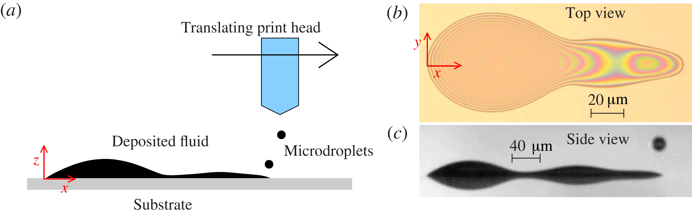
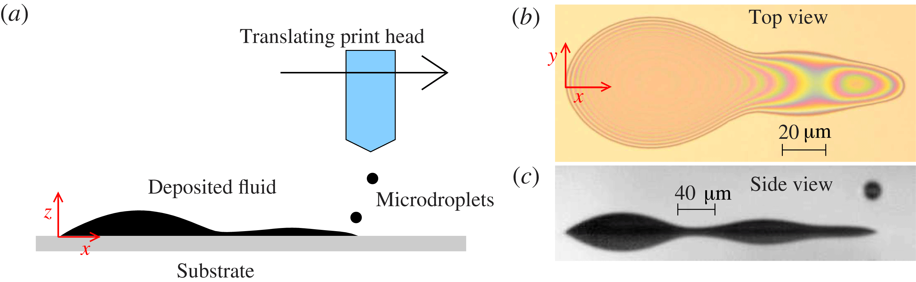
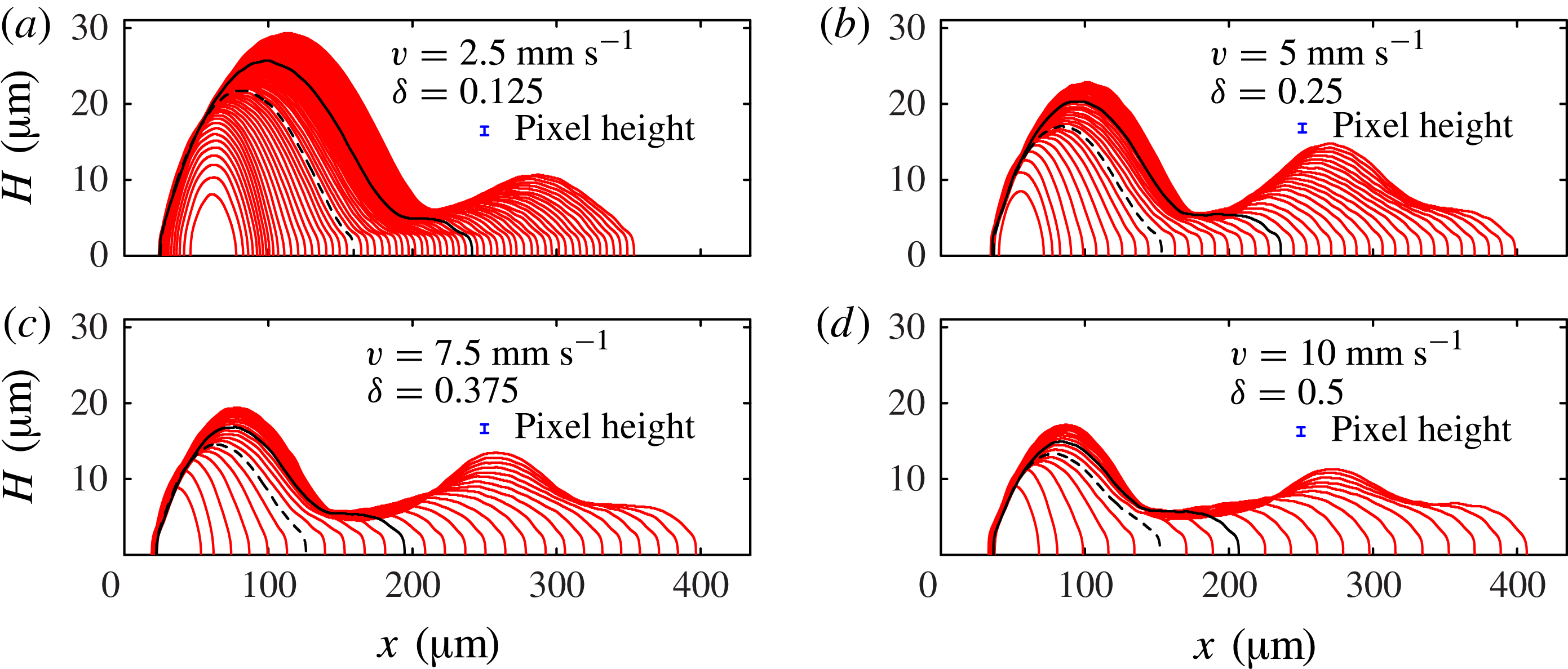
Here we use a combination of experiments and modelling to study a fundamental process in additive manufacturing: the consecutive deposition of a line of equally spaced, overlapping droplets onto a flat solid substrate. The motivating application is the use of ink-jet technology to print polymer organic light-emitting diode (p-OLED) displays, where a short, continuous, uniform line of polymer is required for each pixel. Our experiments were performed at Cambridge Display Technology Limited (CDT), and a Photron Fastcam SA5 digital high-speed camera fitted with long distance magnifying optics (Navitar) was used to record backlit images of the fluid side profile at 100 000 fps; our experimental set-up is shown in figure 1, and a typical range of results is shown in figure 2.
(a) Schematic diagram showing a side view of the experimental apparatus. (b) Top view of the deposited liquid, which wets a two-dimensional region of the substrate that we call the fluid footprint. The boundary of the footprint is the contact line, where air, fluid and substrate meet. (c) Snapshot of our high-speed images of the deposited liquid, showing the side view of the deposited liquid, and also its reflection in the substrate. We use edge-detection algorithms on side-view images such as (c) and those shown in figure 2 to determine the profile height, yielding the side-view profiles shown in figure 3.
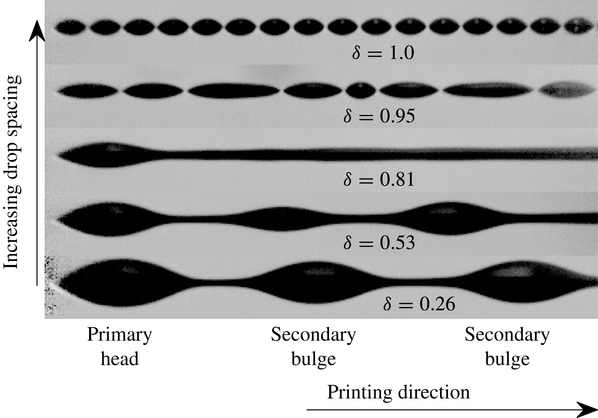
Side-view images (with reflection in substrate) of long printed lines. The centre-to-centre drop spacing ranges from 9 to
 $35\ {\rm\mu}\text{m}$
; each island in the top row is formed from a single printed drop.
 ${\it\delta}$
is proportional to the drop spacing and is defined in the text.
The deposited fluid never adopts a uniform configuration; instead a range of non-uniform morphologies is observed. For a given fluid, substrate and drop size, the observed morphology is principally dependent on the spacing between each drop, characterised by the parameter
 ${\it\delta}={\rm\Delta}x/(2R_{c})$
, where
 ${\rm\Delta}x$
is the centre-to-centre drop spacing and
 $R_{c}$
is the radius of a single drop at rest on the substrate. Each new drop merges very quickly with the deposited fluid; no splashing, oscillations or satellite drop formation is discernible at our frame rate. If
 ${\it\delta}=0$
, the drops are deposited concentrically; if
 ${\it\delta}\gtrapprox 1$
, the drops do not come into direct contact on the substrate but might interact through vapour-based mechanisms (Stringer & Derby Reference Stringer and Derby2010).
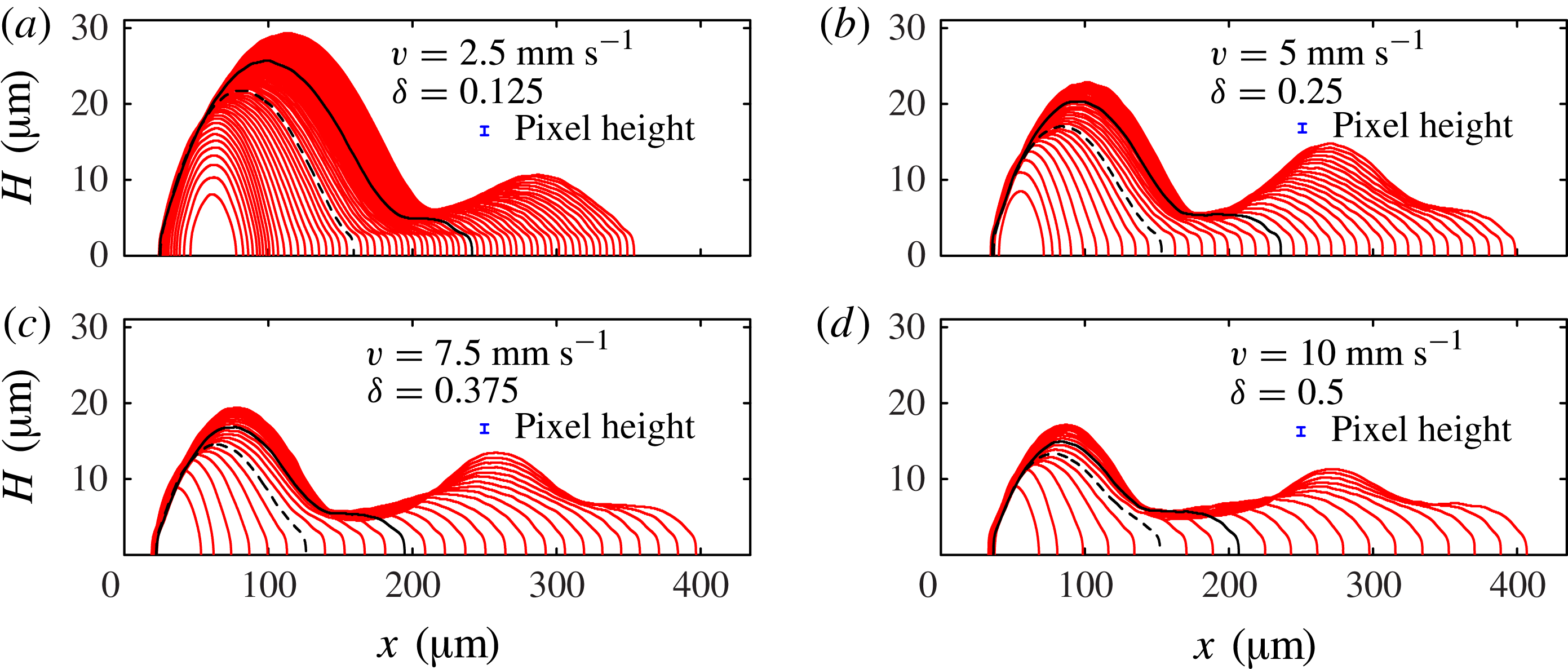
Side-view profiles of the deposited liquid extracted from images such as figure 1(c) just before each new drop is printed. The sequences in (a–d) are for different values of the drop spacing
 ${\rm\Delta}x$
, achieved by changing the horizontal head speed
 $v$
, showing profiles for the first 64, 38, 27 and 20 drops, respectively. In this figure only, the height scale is expanded for ease of visibility. We define
 $N$
as the number of printed drops. In each sequence we have marked profiles at
 $N_{1}$
(dashed black line), where the side profile is no longer convex and
 $N_{2}$
(solid black line), where the side profile first develops a second local maximum. The vertical error bars indicates the height of 1 pixel in our original images, which corresponds to
 $1.16\ {\rm\mu}\text{m}$
.
For small
 ${\it\delta}$
(bottom of figure 2), the droplets form a connected line with a distinctive initial wide bulge or ‘primary head’, followed by a sequence of secondary bulges, each much larger than any individual droplet. Thus, short lines are dominated by the large primary head, as shown in figure 1(b,c). As the drop spacing increases, both primary head and secondary bulges become less pronounced. At
 ${\it\delta}=0.81$
in figure 2, there is still a distinct primary head, but the fluid after the primary head appears to be relatively uniform when viewed from the side. However, top views at comparable
 ${\it\delta}$
show significant scalloped non-uniformities at the same wavelength as the drop spacing (Dalili et al.
Reference Dalili, Chandra, Mostaghimi, Fan and Simmer2014). For yet greater droplet spacing the fluid disconnects to form separate islands. The number of drops within each island generally decreases with further increase in drop spacing, but the precise morphology becomes extremely sensitive to small perturbations. In fact, sensitivity to fluctuations in droplet position (see § 2) was observed for
 ${\it\delta}\gtrsim 0.6$
, leading to isolated and unpredictable disconnections. Once
 ${\it\delta}\gtrapprox 1$
, the individual drops never merge.
Previous theoretical studies have focused on periodic instabilities of uniform lines of fluid (Davis Reference Davis1980; Schiaffino & Sonin Reference Schiaffino and Sonin1997; Stringer & Derby Reference Stringer and Derby2010), but we believe these models are inappropriate here because frame-by-frame analysis shows that the fluid is never in the uniform state. Instead, the fluid evolution must be considered after each drop is placed. Indeed, the configuration shown in figure 3(d) should lie in a stable printing regime according to a uniform line analysis (Stringer & Derby Reference Stringer and Derby2010), but yet there is a pronounced primary head and second bulge, as correctly captured by the new model that we will derive in § 3.3. In a related analysis, Duineveld (Reference Duineveld2003) showed that the existence of one bulge typically leads to further bulge formation through a viscous mechanism. He hypothesised that the initial drops join together to form a bulge that acts as a seed for future development, but did not explore the origin of the initial bulge nor formulate a closed predictive model.
Our intention here is to develop reduced-dimensional models that are flexible enough to allow the ink line shape to evolve naturally; this natural evolution has previously only been achieved in full three-dimensional (3D) simulations which are at present too costly to explore the interactions of more than a few printed drops. We are particularly concerned with ink morphology in relatively short lines, and for these lines the early evolution of the first drops in each line has a persistent effect on subsequent dynamics.
We show that the detailed drop-by-drop fluid morphology observed in our experiments (§ 2) can be quantitatively predicted by models invoking surprisingly few physical mechanisms: surface tension and contact line hysteresis alone predict primary head formation (§ 3.2); while secondary bulges require a competing effect of fluid viscosity (§ 3.3). The detailed impact dynamics can be lumped into an experimentally measurable parameter that characterises the droplet configuration immediately after the fast impact (§ 3.1), but before slower surface-tension-driven spreading. Contact line motion is controversial because the classical continuum model leads to a stress singularity (Huh & Scriven Reference Huh and Scriven1971; Snoeijer & Andreotti Reference Snoeijer and Andreotti2013). We avoid this problem by using a ‘quasi-static’ spreading law described in § 3. We perform a direct comparison between models and experiments in § 3, and in § 4, we discuss when our models are expected to break down, and the implications for the printing of uniform lines. The good quantitative agreement between our experimental and theoretical results, despite substantial simplifying assumptions for both droplet impact and contact line motion, establishes our drop-by-drop modelling approach as a promising theoretical tool that may be extended to gain insight into additional physical effects such as evaporation, substrate topography and wettability variations.
2. Experiments
The piezoelectric drop-on-demand ink-jet print head (Spectra SX3, Fujifilm Dimatix) produced drops with volume
 $V_{0}=4.6\pm 0.3\ \text{pl}$
at a deposition frequency
 $f=540\ \text{Hz}$
. The centre-to-centre drop spacing
 ${\rm\Delta}x$
was controlled by varying the horizontal printhead speed
 $v=f{\rm\Delta}x$
in the range
 $2.5{-}50\ \text{mm}\ \text{s}^{-1}$
. At impact, the drops have vertical speed
 $U_{i}=2.2\ \text{m}\ \text{s}^{-1}$
and are close to spherical, with radius
 $R_{f}=10.3\ {\rm\mu}\text{m}$
. Fluctuations in the position of the centre of mass of each droplet after impact were less than
 $1\ \text{pixel}=1.16\ {\rm\mu}\text{m}$
, i.e. less than 5 % of the initial droplet diameter, when measured in a sequence of disconnected droplets for
 ${\it\delta}\gtrapprox 1$
. The ink used is a CDT proprietary solution used in p-OLED printing, with dynamic viscosity
 ${\it\mu}=6.25\times 10^{-3}\ \text{Pa}\ \text{s}$
, density
 ${\it\rho}=1.066\times 10^{3}\ \text{kg}\ \text{m}^{-3}$
and surface tension
 ${\it\sigma}=44\times 10^{-3}\ \text{N}\ \text{m}^{-1}$
.
For a drop lying on the substrate, the fluid configuration with minimum energy is a spherical cap with constant contact angle
 ${\it\theta}$
. The persistence of non-spherical interfaces long after deposition is a consequence of contact angle hysteresis, where a stationary contact line is possible whenever
 ${\it\theta}_{R}<{\it\theta}<{\it\theta}_{A}$
, where
 ${\it\theta}_{A}$
is the advancing angle and
 ${\it\theta}_{R}$
is the receding angle. Contact angle hysteresis occurs on a wide variety of substrates due to the presence of surface defects. For liquid suspensions, hysteresis leads to the coffee-ring effect (Deegan et al.
Reference Deegan, Bakajin, Dupont, Huber, Nagel and Witten2000), which further enhances the contact line pinning.
In our experiments, the substrate is ozone-treated, indium–tin oxide (ITO)-coated glass. The deposition of the CDT proprietary solution is associated with significant contact angle hysteresis, where
 ${\it\theta}_{A}$
increases with the age of the substrate. Immediately after ozone treatment of the surface,
 ${\it\theta}_{A}$
is very low, and the fluid spreads into a wide, circular puddle which is sufficiently thin that variations in the layer height are within the tolerance of 1 pixel =
 $1.16\ {\rm\mu}\text{m}$
. In this study, we restrict our attention to an ‘aged’ substrate (i.e. where the time elapsed since ozone treatment is more than 4 weeks) for which
 ${\it\theta}_{A}\approx 50\pm 2^{\circ }$
and
 ${\it\theta}_{R}<4^{\circ }$
, and our images reveal significant non-uniformity in the fluid profile, such as shown in figure 1(c). This value of
 ${\it\theta}_{A}$
leads to the radius of a single drop at rest
 $R_{c}=18.0\pm 0.2\ {\rm\mu}\text{m}$
. Hereinafter, we concentrate on results for the dimensionless separation parameter
 ${\it\delta}={\rm\Delta}x/(2R_{c})$
in the range
 $0.125{-}0.5$
to avoid the geometric sensitivities due to droplet-position fluctuations observed at larger
 ${\it\delta}$
.
Figure 3 shows superimposed side profiles just before each new drop is printed (every
 $1/540$
s). To extract the profiles from the raw experimental images, we analyse each column of the image, and fit a hyperbolic tangent profile to the image intensity as a function of vertical position. This allows us to determine the position of the top edge and its reflection in the substrate, and we use the reflective symmetry of the image to ensure that the horizontal centreline is aligned between frames. When the fluid evolution is sufficiently rapid (certainly the case for the initial drops, see figure 4) these are the static fluid profiles that develop after each drop is added. The first few drops merge into a single bulge that is approximately elliptical when viewed from above. We define
 $N$
to be the number of deposited drops. At
 $N=N_{1}$
, an elongated shallow rivulet forms connecting a primary head to the moving deposition point and the profile is no longer convex. At
 $N=N_{2}$
, the profile develops a second local maximum, corresponding to a secondary bulge in the top view (similar to that shown in figure 1
b); the primary head stops growing some time after the secondary bulge begins to form. For all
 ${\it\delta}$
, a large primary head forms near the start of the line, which moves very little after the first few drop impacts.
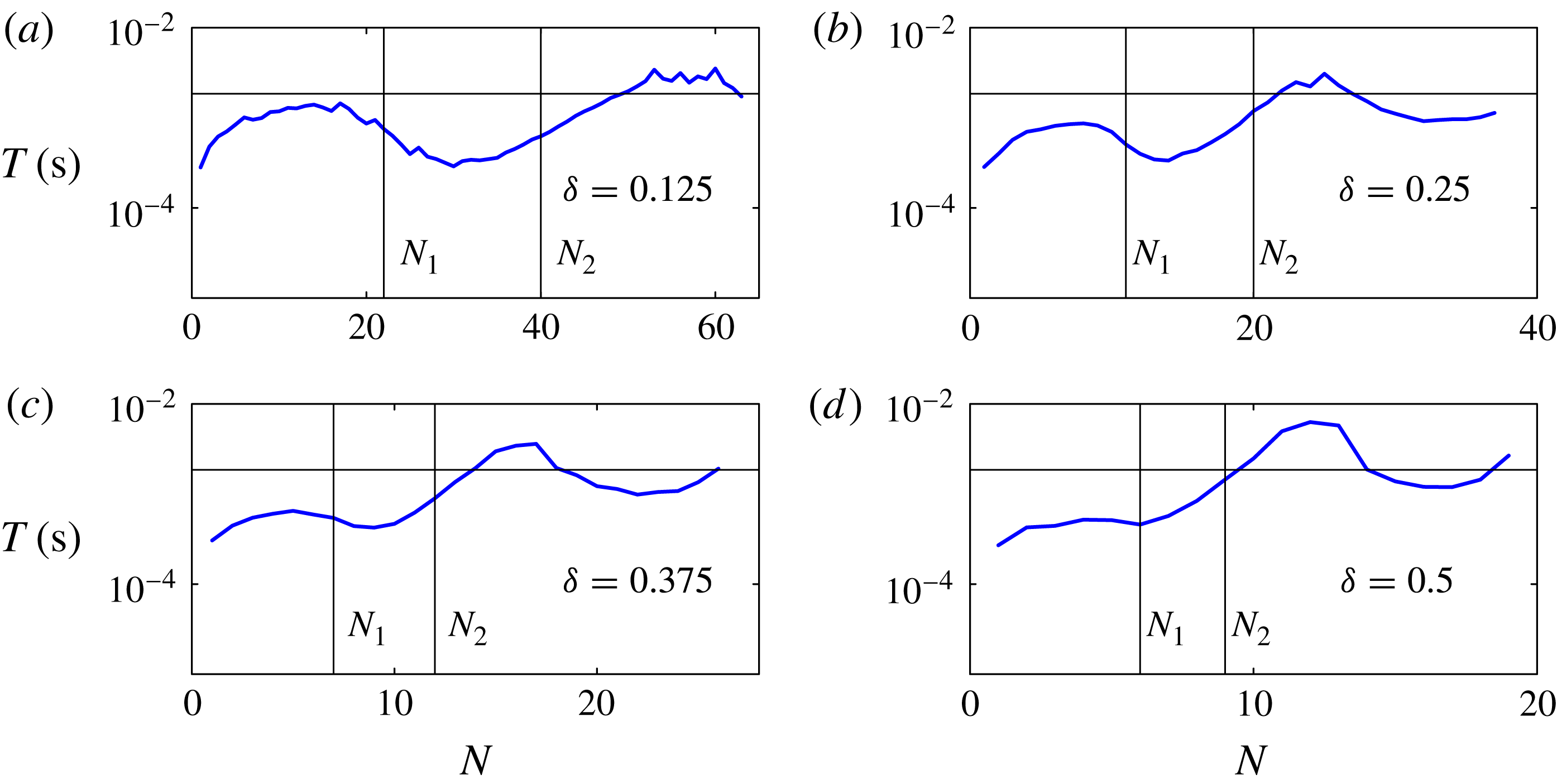
Characteristic timescale for the ink response to each printed drop, based on exponential fits to the evolution of the total area of ink viewable in the side-view images such as shown in figure 1(c) in the 180 frames after the initial impact of each drop, but before the next drop arrives. The vertical lines indicate drop numbers
 $N_{1}$
and
 $N_{2}$
at which an elongated rivulet, and a second local maximum are respectively first discernible. The horizontal line marks the interval
 $T_{p}=1.9\times 10^{-3}\ \text{s}$
at which successive drops are printed.
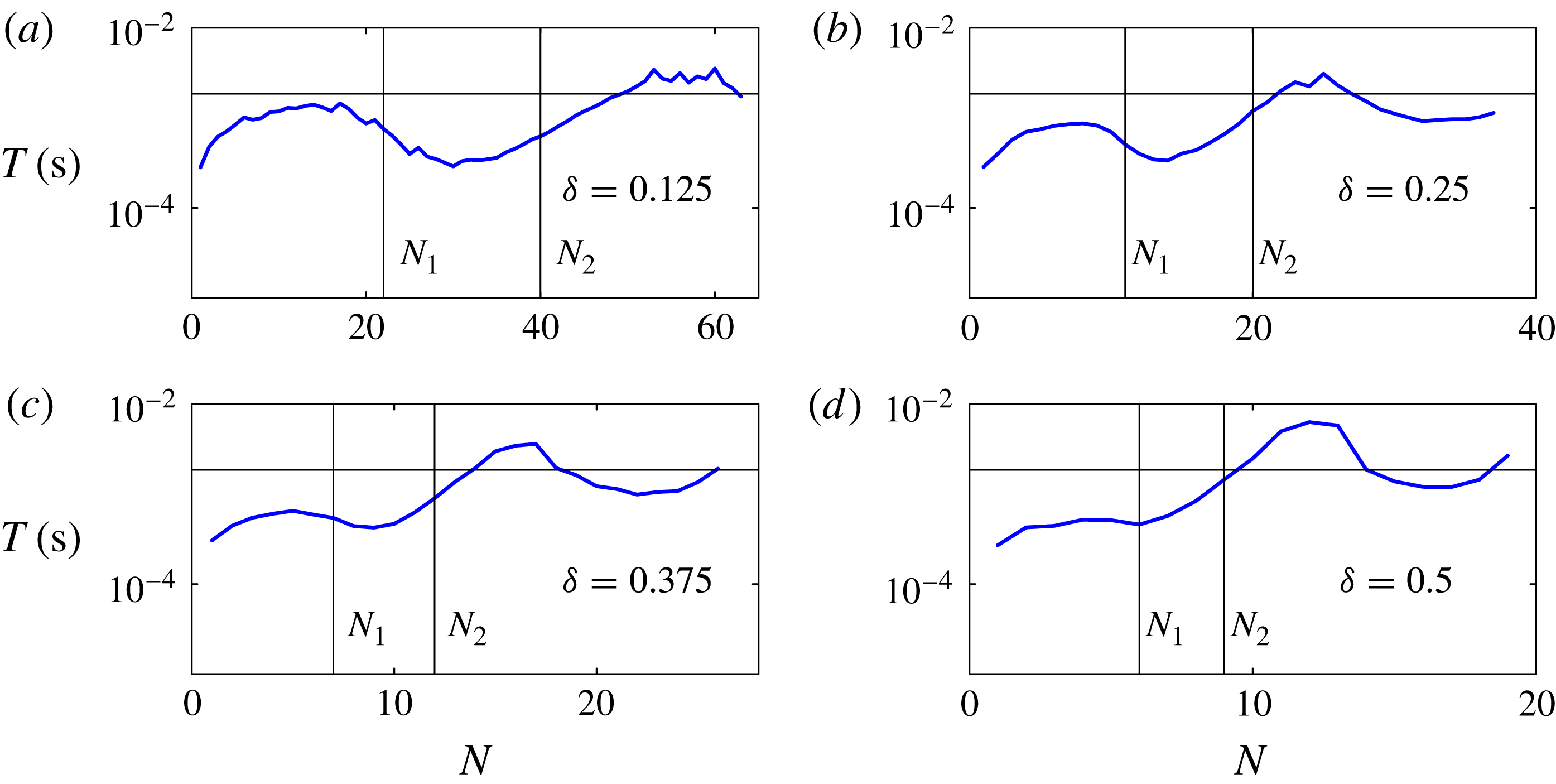
The complete evolution can be viewed in the supplementary movies available at http://dx.doi.org/10.1017/jfm.2014.621, which are analysed to estimate the characteristic timescales over which the fluid reacts to each printed drop. After impact, the first drops in each line are quickly absorbed into the quiescent fluid, over less than five frames at this frame rate. Figure 4 shows timescales
 $T(N)$
obtained by fitting an exponential decay to the area of ink visible in the side-view images as a function of time, based on the 180 frames between droplet arrivals given the deposition frequency of 540 Hz and frame rate of 100 000 fps, but excluding the first five frames for each drop. In each sequence, the measured
 $T$
is much smaller than the printing period
 $T_{p}=1/f$
for the first few drops, but soon becomes comparable to
 $T_{p}$
, suggesting that different physical processes are starting to dominate the dynamics. The measured timescale
 $T$
continues to vary as
 $N$
increases, even once a second local maximum in the profile height has appeared at
 $N_{2}$
. The maximum value of
 $T$
is around
 $4\times 10^{-3}\ \text{s}$
, which is greater than the drop deposition time interval. As
 ${\it\delta}$
increases, the value of
 $N$
at which
 $T$
becomes comparable to
 $T_{p}$
decreases. This contributes to growing sensitivity to perturbations as
 ${\it\delta}$
increases.
3. Simplified models
Line printing depends on a wide range of physical parameters including the mechanical properties set by the printing system (i.e. drop size, impact velocity and spacing), the material properties of the printing liquid and its vapour, and the properties associated with the interaction of the printing liquid with the substrate. The physical mechanisms governing contact-line motion are not yet fully established, but a significant number of parameters may be required to describe the motion of the contact-line. A simple Navier-slip model would at least require a slip length, advancing and receding contact angles, and the functional dependence of the dynamic contact angle on the contact-line speed.
Direct 3D numerical simulations of impact, deposition and spreading have been performed for up to four successive printed drops (Lee & Son Reference Lee and Son2011; Graham, Farhangi & Dolatabadi Reference Graham, Farhangi and Dolatabadi2012) but the scale of the computational effort prohibits both simulation of a wide range of parameters and extension to longer printed lines. Our aim is to show that the essential post-impact dynamics can be quantitatively captured by much simpler models based on a few key physical mechanisms, which dominate on the relatively slow time scale that characterises fluid redistribution and spreading on the substrate.
We use thin-film, incompressible, fluid mechanics to describe the drop-scale motion, and introduce Cartesian coordinates such that the fluid lies in the region
 $z=0$
(the substrate) to
 $z=h(x,y)$
(the interface). We define the footprint
 ${\rm\Omega}(t)$
to be the two-dimensional region where fluid and substrate meet.
We focus on modelling the continuous spreading that occurs in the intervals between the deposition of each droplet. The experimental timescale analysis shown in figure 4 suggests that the physical processes underlying the dynamics of the initial drops are different from those controlling the behaviour of subsequent drops. We find that viscous effects are not required to understand the post-impact fluid redistribution of the first few drops; and we develop a model (Model I) for this regime by taking the limit where surface tension is so strong that the interface curvature is spatially constant and the fluid rearranges itself instantaneously to reach equilibrium for any given contact-line position. As suggested by figure 4, additional physical mechanisms are required to understand the later dynamics and we develop a second model (Model II), in which the speed of fluid redistribution within the footprint is set by a balance between surface tension and viscosity. Although the physical mechanisms in Model II are the same as in the model of Duineveld (Reference Duineveld2003), our model can be used predictively because the assumptions made about the fluid geometry are less prescriptive.
We assume ‘quasi-static’ spreading, where viscous dissipation only occurs very close to the contact line; and the interface shape is the same as if the contact line were static. For simplicity, we choose a piecewise linear spreading law with zero receding angle:
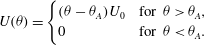 $$\begin{eqnarray}\displaystyle U({\it\theta})=\left\{\begin{array}{@{}ll@{}}({\it\theta}-{\it\theta}_{A})U_{0}\quad & \text{for }{\it\theta}>{\it\theta}_{A},\\ 0\quad & \text{for }{\it\theta}<{\it\theta}_{A}.\end{array}\right. & & \displaystyle\end{eqnarray}$$
The experimental receding contact angle is not zero, but when
 ${\it\delta}\leqslant 0.5$
the contact lines did not recede (the receding angle was always exceeded). Based on our contact angle goniometry measurements, we use the value
 $U_{0}=0.01\ \text{m}\ \text{s}^{-1}\ \text{rad}^{-1}$
, although these measurements only span variations of approximately 10 % in the advancing contact angle and we apply the spreading law in our models for contact angles up to twice the static advancing contact angle. We note that the commonly used Cox–Voinov law (Snoeijer & Andreotti Reference Snoeijer and Andreotti2013) would give
 $U_{0}\approx 0.3\ \text{m}\ \text{s}^{-1}\ \text{rad}^{-1}$
. This law is derived for the case of a pure fluid spreading on a flat substrate, with zero contact angles, but also holds surprisingly well in experiments with contact angles of up to 70–80° in the absence of hysteresis (Bonn et al.
Reference Bonn, Eggers, Indekeu, Meunier and Rolley2009). The reason for the significant deviation in contact-line speed
 $U_{0}$
between our system and the Cox–Voinov law is not clear, but contact angle hysteresis of
 ${\it\theta}_{A}-{\it\theta}_{R}\approx 50^{\circ }$
is quite large, and our printing fluid is not pure (as is the case for most applications involving deposition of a functional liquid). However, we find that our results are only weakly dependent on
 $U_{0}$
, as discussed in more detail for Models I and II in §§ 3.2 and 3.3, respectively. Naturally, more complex spreading laws could be included within the model framework.
3.1. Initial conditions due to impact of individual printed droplets
The presence of contact-angle hysteresis means that the final resting state depends on the initial conditions, which are chosen to approximate the successive printing of individual droplets. The initial conditions that are relevant for our models are the shape and location of the new wetted area, the increase in total fluid volume, and for Model II, the distribution of the fluid within the wetted area.
Visser et al. (Reference Visser, Tagawa, Sun and Lohse2012) describe several stages of impact of a single drop on a dry substrate. Prior to impact, the air layer between falling drop and substrate becomes strongly squeezed. The drop spreads over this air layer, reaching a maximum spreading radius before making contact with the substrate at its outer edge. Splashing may occur as the drop spreads over the layer, but is typically not observed in microscale experiments (Visser et al. Reference Visser, Tagawa, Sun and Lohse2012). During spreading over the air layer, the fluid is not in contact with the substrate. Hence, the maximum spreading radius can be limited either by viscosity or surface tension, but is only weakly dependent on the substrate properties such as contact angle.
In our experiments, the Weber and Reynolds numbers at impact have values of
 $\mathit{We}=2{\it\rho}\,R_{f}U_{i}^{2}/{\it\sigma}=2.4$
and
 $\mathit{Re}=2{\it\rho}\,R_{f}U_{i}/{\it\mu}=7.7$
. The results compiled by Visser et al. (Reference Visser, Tagawa, Sun and Lohse2012) from a variety of experimental studies indicate that our impacts are towards the lower end of the range of both
 $\mathit{We}$
and
 $\mathit{Re}$
, and thus may be interpreted as slow. Within this limit, the measurements of the maximum spreading radius presented by Visser et al. saturate at approximately 1.3 times the radius of the falling drop. In our experiments, the falling radius is
 $R_{f}=10.3\ {\rm\mu}\text{m}$
so that the maximum spreading radius achieved during impact would be
 $R_{i}=1.3\,R_{f}=13.4\ {\rm\mu}\text{m}$
based on this estimate. The radius
 $R_{i}$
is smaller than the contact radius
 $R_{c}=18.0\ {\rm\mu}\text{m}$
of a spherical cap with contact angle
 ${\it\theta}={\it\theta}_{A}$
. This implies that a single drop has a contact angle larger than
 ${\it\theta}_{A}$
at impact, and so will spread axisymmetrically until it reaches radius
 $R_{c}$
, at which point the contact line stops moving.
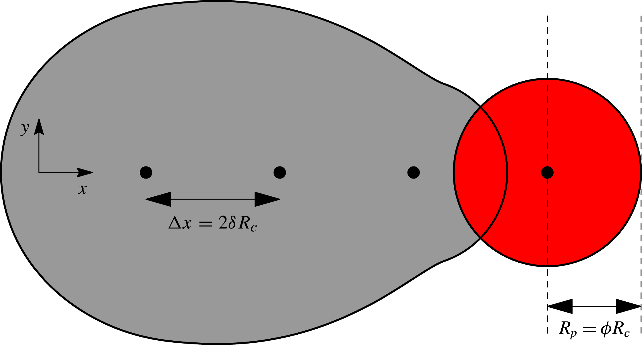
The first drop in each printed line lands on dry substrate, but the impacts of the second and subsequent drops are likely to be affected by interactions with the preexisting fluid layer. Full resolution of the interactions would require significant computation and will depend on modelling assumptions used to describe the incompletely understood physics. Instead, we approximate the impact process by choosing initial conditions for spreading according to a simple scheme that imitates the printing of circular, offset drops. When a new drop is printed, its volume
 $V_{0}$
is distributed over a circular region of radius
 $R_{p}$
offset in the
 $x$
direction by a distance
 ${\rm\Delta}x$
from the previous drop. The footprint
 ${\rm\Omega}$
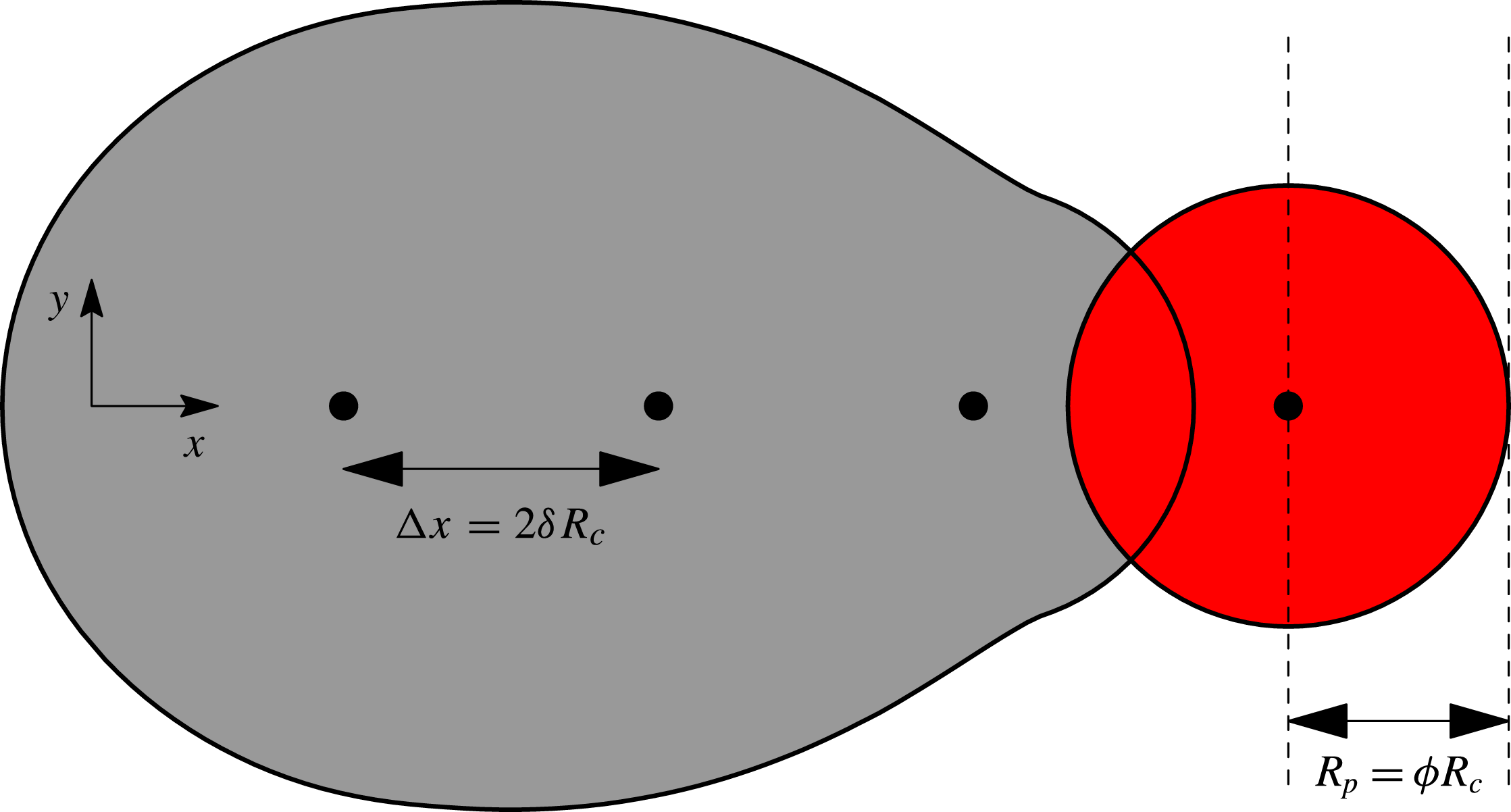
is then the union of all wetted regions and we increment the total volume accordingly. This scheme is illustrated in figure 5. Effectively, we lump the effects of drop impact into a single measurable parameter that sets the size
 $R_{p}$
of the circular region that each drop is spread over. In principle, the parameter could be determined from full impact simulations, but experimental measurement avoids the problem of modelling-assumption dependence.
An illustration of our scheme for ‘printing’ individual droplets. The centres of the drops are located at the filled black circles, each separated by a distance
 ${\rm\Delta}x=2{\it\delta}R_{c}$
from the previous drop. To determine the initial conditions for evolution just after drop impact, we spread the volume of each drop over a radius
 $R_{p}={\it\phi}R_{c}$
. We take the wetted area to be the union of the shaded regions. We calculate the dimensionless spreading parameter
 ${\it\phi}$
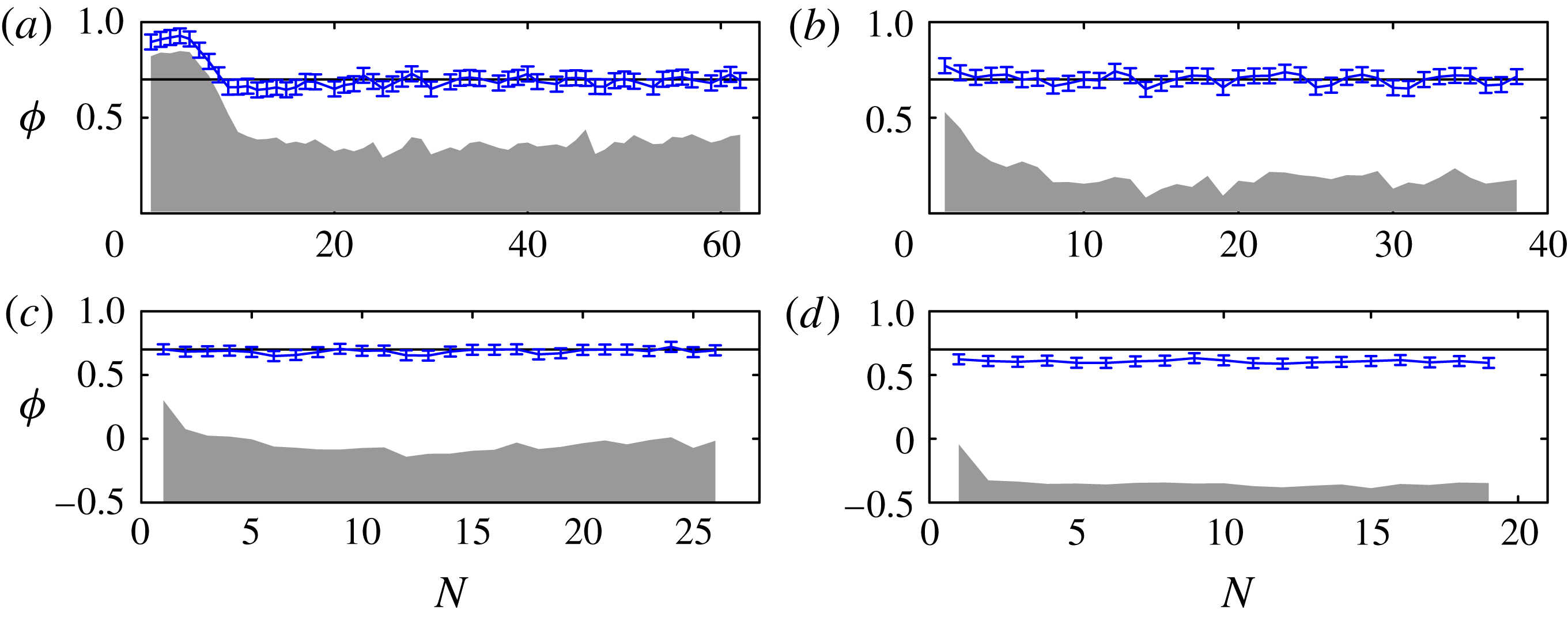
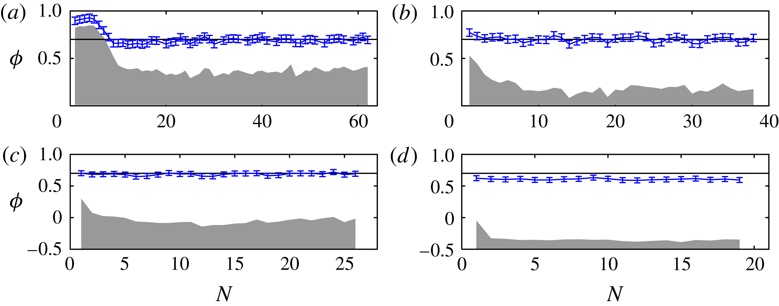
from our side-view experiments by measuring the distance between the dashed lines, i.e. the horizontal distance between the maximum extent of the fluid and the centre of the just-impacted drop. The values of
 ${\it\phi}$
measured in this way from our experiments are shown in figure 6.
Measurements of
 ${\it\phi}$
from each impact in our experiments, with (a–d) corresponding to figure 3. The error bars show the average contact-line position in the first five frames after each impact. The centre of the falling drop is at
 ${\it\phi}=0$
. The shaded region indicates the extent of the wetted region just before each impact; the centre of the falling drop is above the wetted region for (a,b), very close to the edge in (c), and above dry substrate in (d). The horizontal line indicates the value
 ${\it\phi}=0.7$
which we use in all our simulations except for the results for
 ${\it\phi}=1$
shown in figures 8 and 16.
We define the printing radius
 $R_{p}={\it\phi}R_{c}$
as the contact radius of the drop after initial impact, but before significant interaction with the sessile fluid. Detailed studies of impact dynamics when
 $N=2$
have shown that the spreading parameter
 ${\it\phi}$
can take a wide range of values (Graham et al.
Reference Graham, Farhangi and Dolatabadi2012; Lee et al.
Reference Lee, Kim, Chandra and Yoon2013). As our printed lines are substantially longer than in these detailed studies, we choose
 ${\it\phi}$
based on measurements from our experimental videos. To do so, we measure
 $R_{p}$
as the distance in the
 $x$
direction between the centre of mass of the impacting drop and the contact-line extent just after impact (these two locations are marked by dashed lines in figure 5). Figure 6 shows the resulting values for
 ${\it\phi}$
for each impact in the experimental sequences shown in figure 3. After the first few drops for figure 6(a,b), and for all impacts in (c), the results are clustered around
 ${\it\phi}=0.7$
, but in (d), the average value of
 ${\it\phi}$
is slightly lower. Within the margin of error in our measurements of
 ${\it\phi}$
, we note that the value
 ${\it\phi}=0.7$
is equal to the value we would obtain if we set
 $R_{p}=R_{i}=1.3\,R_{f}=0.74R_{c}$
based on Visser et al. (Reference Visser, Tagawa, Sun and Lohse2012). We also note that
 $2^{1/3}\,R_{f}\simeq 0.72R_{c}$
;
 $2^{1/3}$
is the radius ratio between a hemispherical drop and a spherical drop of identical volumes. Thus, the value
 ${\it\phi}=0.7$
can also be interpreted as each impacting drop being reconfigured into a hemisphere immediately post-impact.
The first drop will spread axisymmetrically until it reaches the advancing contact angle, so for the first drop, we set
 $R_{p}=R_{c}$
, the resting radius of a single drop. For subsequent drops, however, we set
 $R_{p}={\it\phi}R_{c}$
. As
 ${\it\phi}$
is largely independent of
 $N$
, we choose to use
 ${\it\phi}=0.7$
throughout the simulations, but we will also show selected results for
 ${\it\phi}=1$
. We would expect
 ${\it\phi}$
to increase for larger values of
 ${\it\delta}$
because the fluid will spread until either it comes into contact with the resting fluid, giving
 ${\it\phi}\geqslant {\it\delta}$
, or the advancing contact angle is reached at
 ${\it\phi}=1$
.
3.2. Model I: Strong surface tension limit
In Model I, we assume that there is no viscous resistance to movement of fluid within the footprint
 ${\rm\Omega}(t)$
. The fluid arranges itself so that pressure is spatially constant. The pressure within the fluid is linked to the interface curvature
 ${\it\kappa}(t)$
by the Young–Laplace equation, so that
 $p={\it\sigma}{\it\kappa}$
, and in the thin-film approximation
 ${\it\kappa}=-{\rm\nabla}^{2}h$
, where
 ${\rm\nabla}^{2}=\partial _{xx}+\partial _{yy}$
. If both
 ${\rm\Omega}$
and total fluid volume
 $V$
are known, we can determine
 $h(x,y,t)$
and
 $p(t)$
by solving the linear equations
 $$\begin{eqnarray}p(t)=-{\it\sigma}{\rm\nabla}^{2}h\quad \text{for }(x,y)\in {\rm\Omega},\quad V=\int _{{\rm\Omega}}h\text{d}x\text{d}y,\end{eqnarray}$$
with boundary condition
 $h=0$
on the contact line.
We calculate the contact angle
 ${\it\theta}$
from
 $\tan {\it\theta}=-\boldsymbol{n}\boldsymbol{\cdot }\boldsymbol{{\rm\nabla}}h$
, where
 $\boldsymbol{n}$
is the two-dimensional (2D) unit normal directed out of
 ${\rm\Omega}$
, and
 $h(x,y)$
is known from the solution of (3.2). Under the small-angle approximation, we use the linear expression
 ${\it\theta}=-\boldsymbol{n}\boldsymbol{\cdot }\boldsymbol{{\rm\nabla}}h$
. We allow the contact line to spread outwards with normal velocity controlled by the spreading law (3.1). Specifically, if a material point on the contact line is at
 $(x,y)=\boldsymbol{R}(t)$
, then
 $$\begin{eqnarray}\boldsymbol{n}\boldsymbol{\cdot }{\displaystyle \frac{\text{d}\boldsymbol{R}}{\text{d}t}}=U({\it\theta})\quad \text{for }{\it\theta}=-\boldsymbol{n}\boldsymbol{\cdot }\boldsymbol{{\rm\nabla}}h.\end{eqnarray}$$
At each time step, we use (3.3) to update the footprint
 ${\rm\Omega}$
, and then recalculate
 $h$
and
 ${\it\theta}$
. Andrieu et al. (Reference Andrieu, Beysens, Nikolayev and Pomeau2002) proposed a similar model for relaxation of near-spherical droplets towards equilibrium, but performed calculations only for circular contact lines. We solve the equations with a second-order accurate implicit scheme using the finite-element library oomph-lib (Heil & Hazel Reference Heil and Hazel2006). The domain is discretised via a triangular mesh that deforms as the ink spreads, and so the mesh boundary remains fitted to the contact line. We can therefore obtain results for arbitrary contact-line shapes.
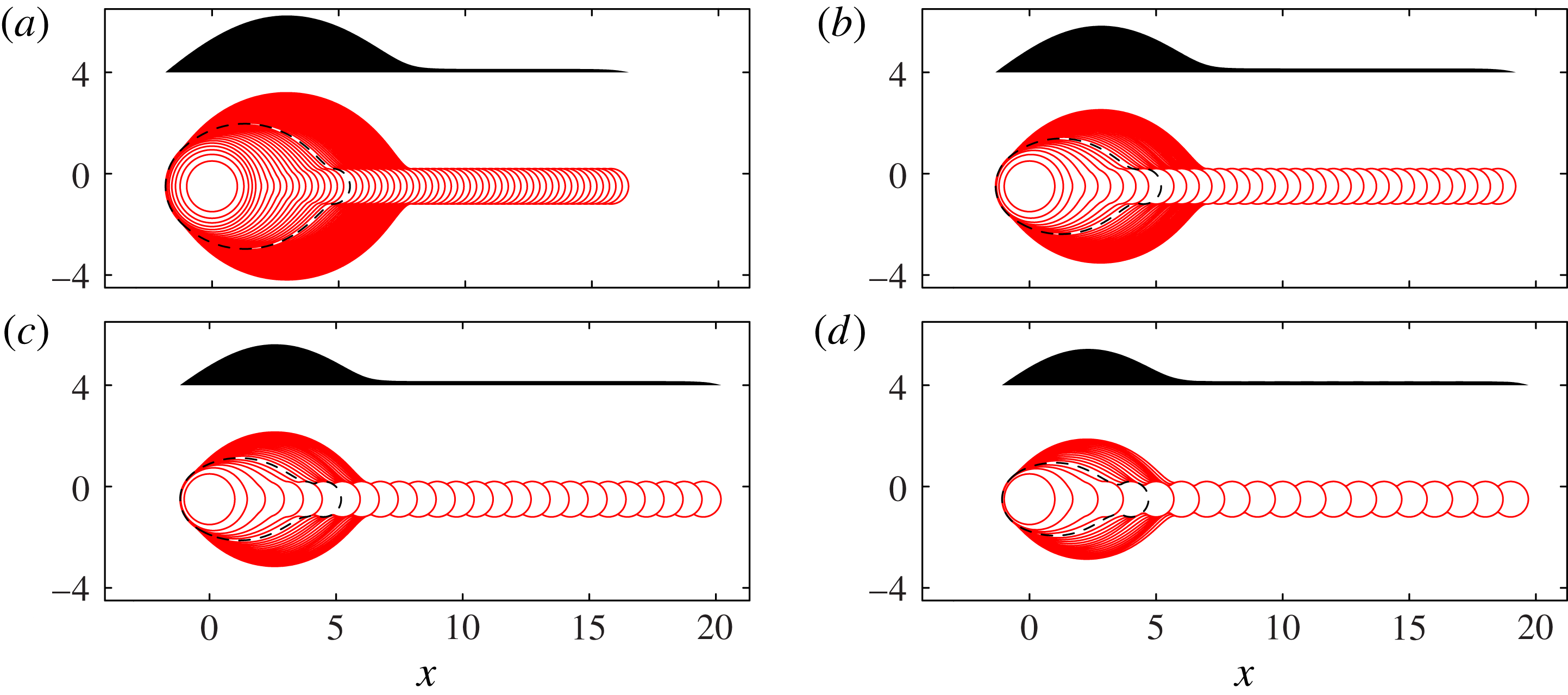
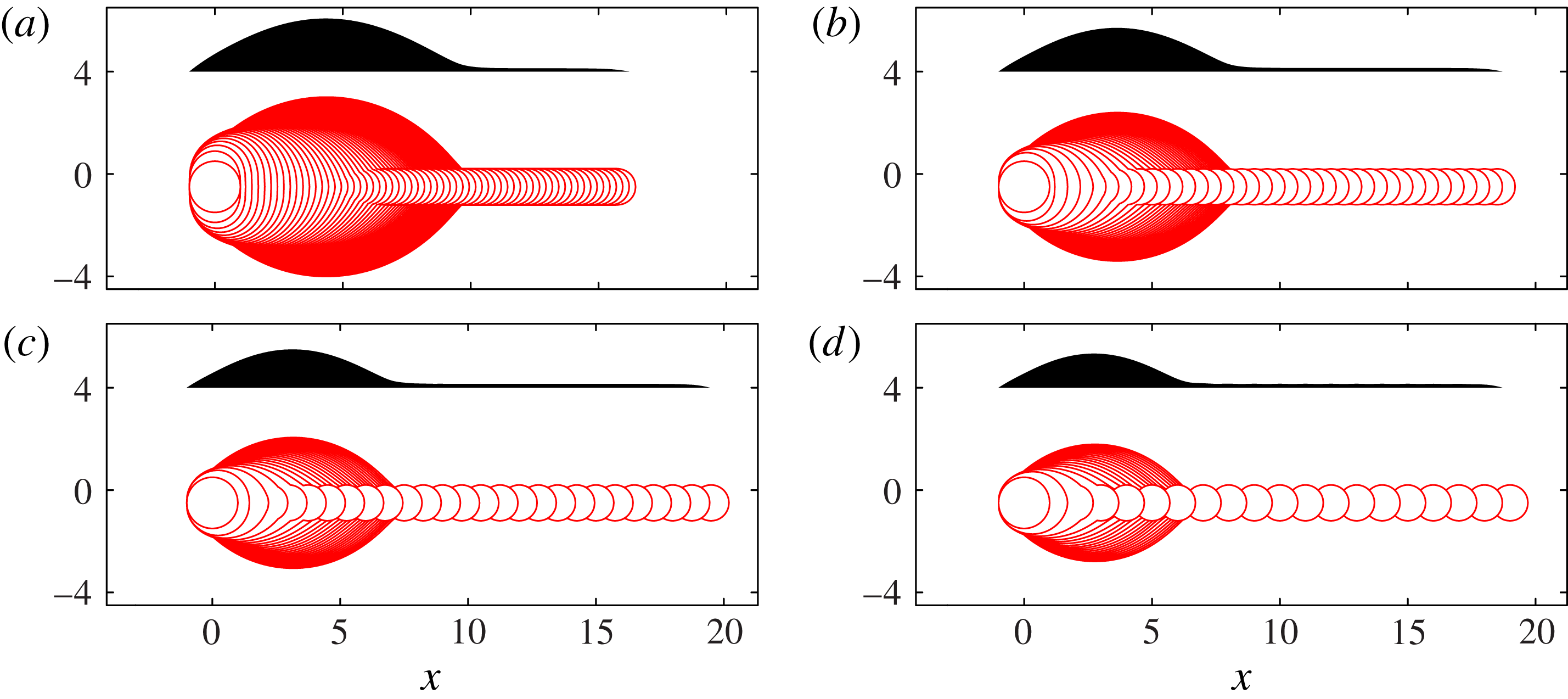
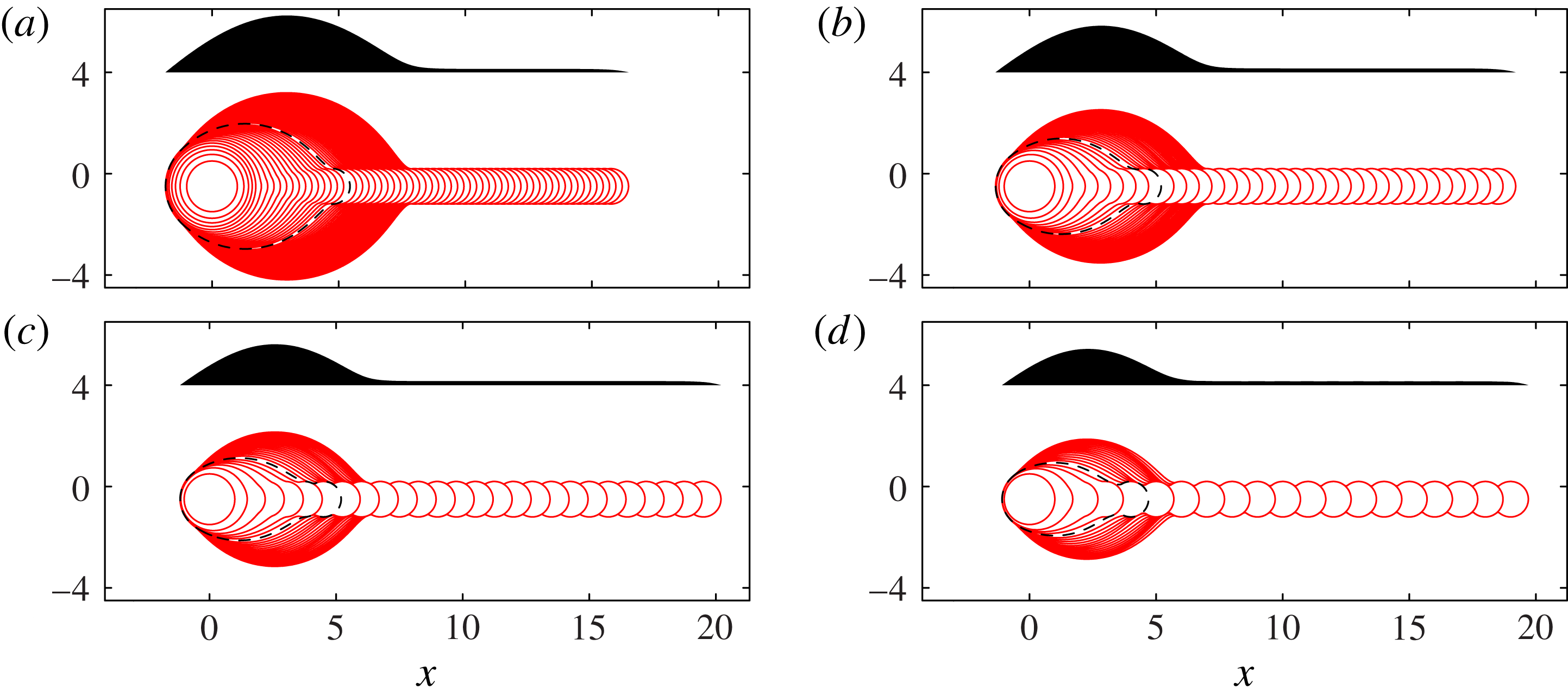
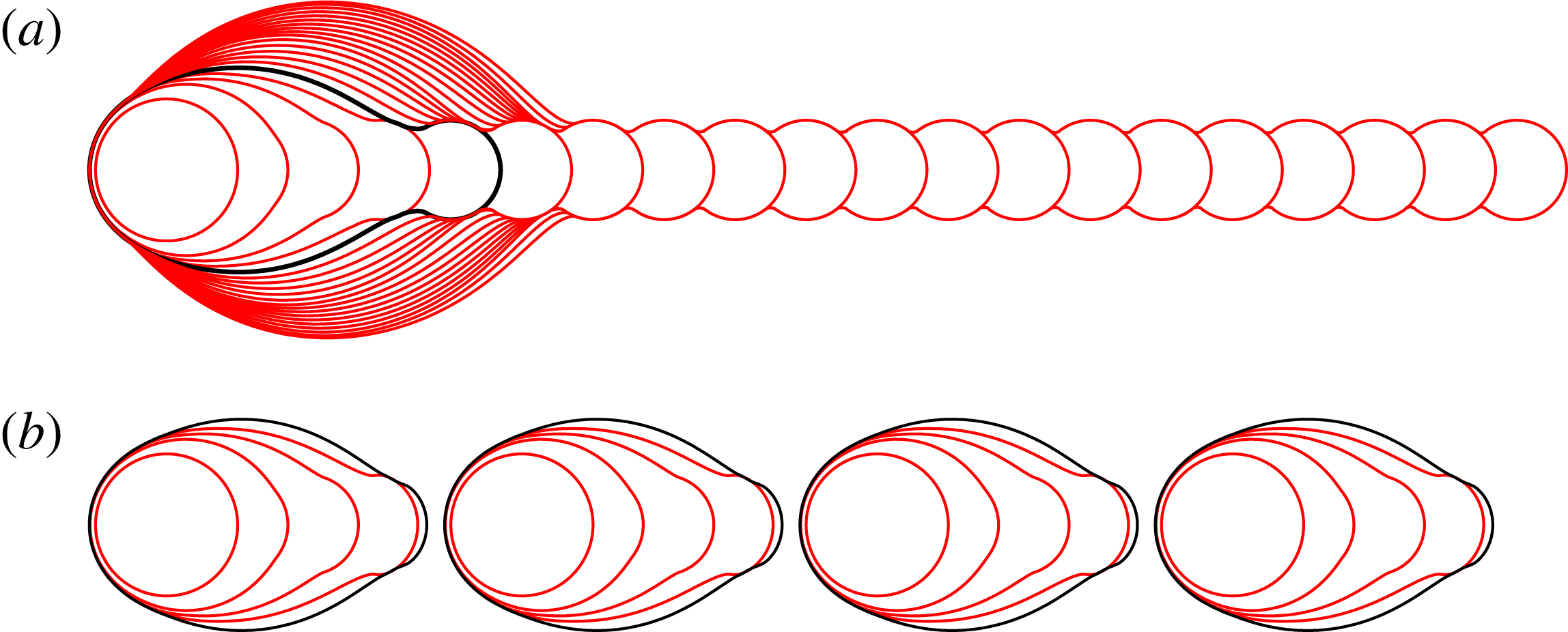
Top- and side-view results from Model I are shown in figure 7. For each value of
 ${\it\delta}$
, the sequence features a growing primary head that connects to a long, shallow rivulet extending to the deposition point. The general behaviour of the primary head is similar to the experimental images, with the head being most pronounced for small
 ${\it\delta}$
. In contrast to the experiments, however, there is no secondary bulge formation for any value of
 ${\it\delta}$
.
Superimposed contact-line positions (solid lines) and final side-view profile (shaded) for Model I, with (a)
 ${\it\delta}=0.125$
, (b)
 ${\it\delta}=0.25$
, (c)
 ${\it\delta}=0.375$
and (d)
 ${\it\delta}=0.5$
, matching figure 3. The dashed line indicates the contact line position at
 $N=N_{1}$
, where the side profile is no longer convex. For this calculation, we have used
 ${\it\phi}=0.7$
, infinite time between printed drops, and a receding angle of zero. Scalloping with the same wavelength as the drop spacing is visible along the edges of the rivulet in (c,d) and is more pronounced for larger
 ${\it\delta}$
. Similar scalloping is seen in the experimental top views shown by Soltman & Subramanian (Reference Soltman and Subramanian2008) for
 ${\it\delta}\approx 0.83$
and by Dalili et al. (Reference Dalili, Chandra, Mostaghimi, Fan and Simmer2014) for
 ${\it\delta}$
in the range 0.5–1, again more pronounced for larger
 ${\it\delta}$
. In this figure and also in figures 8, 11, 13 and 16, all lengths are scaled on
 $R_{c}$
.
For the results of Model I shown in figure 7, sufficient time is allowed between the printing of successive drops so that the contact line always comes to rest before the next drop is deposited, which renders the results independent of
 $U_{0}$
. More generally, in order to construct a timescale for contact-line spreading from
 $U_{0}$
, we use the distance
 $R_{c}$
and typical contact angle
 ${\it\theta}_{A}$
, to reach the dimensional timescale
 $T_{c}=R_{c}/({\it\theta}_{A}U_{0})$
. The competition between this spreading timescale and the period between successive drops
 $T_{p}$
is quantified by the dimensionless time parameter
 ${\it\tau}_{p}=T_{p}/T_{c}$
, which is approximately 1 if
 $U_{0}=0.01\ \text{m}\ \text{s}^{-1}\ \text{rad}^{-1}$
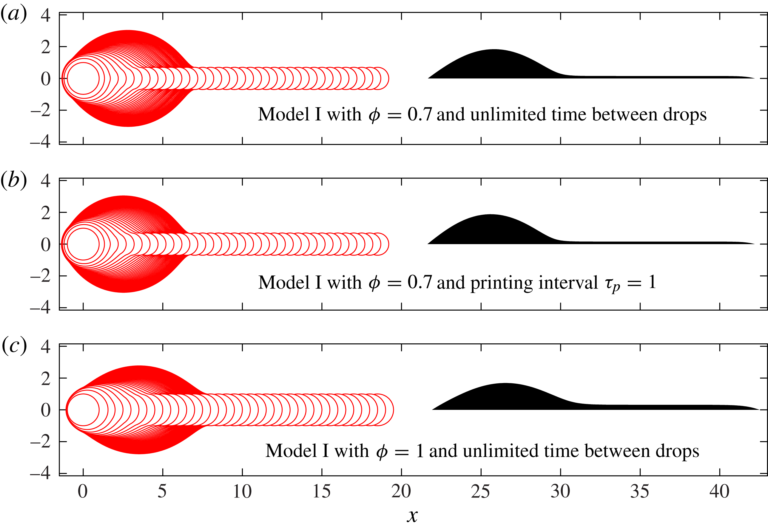
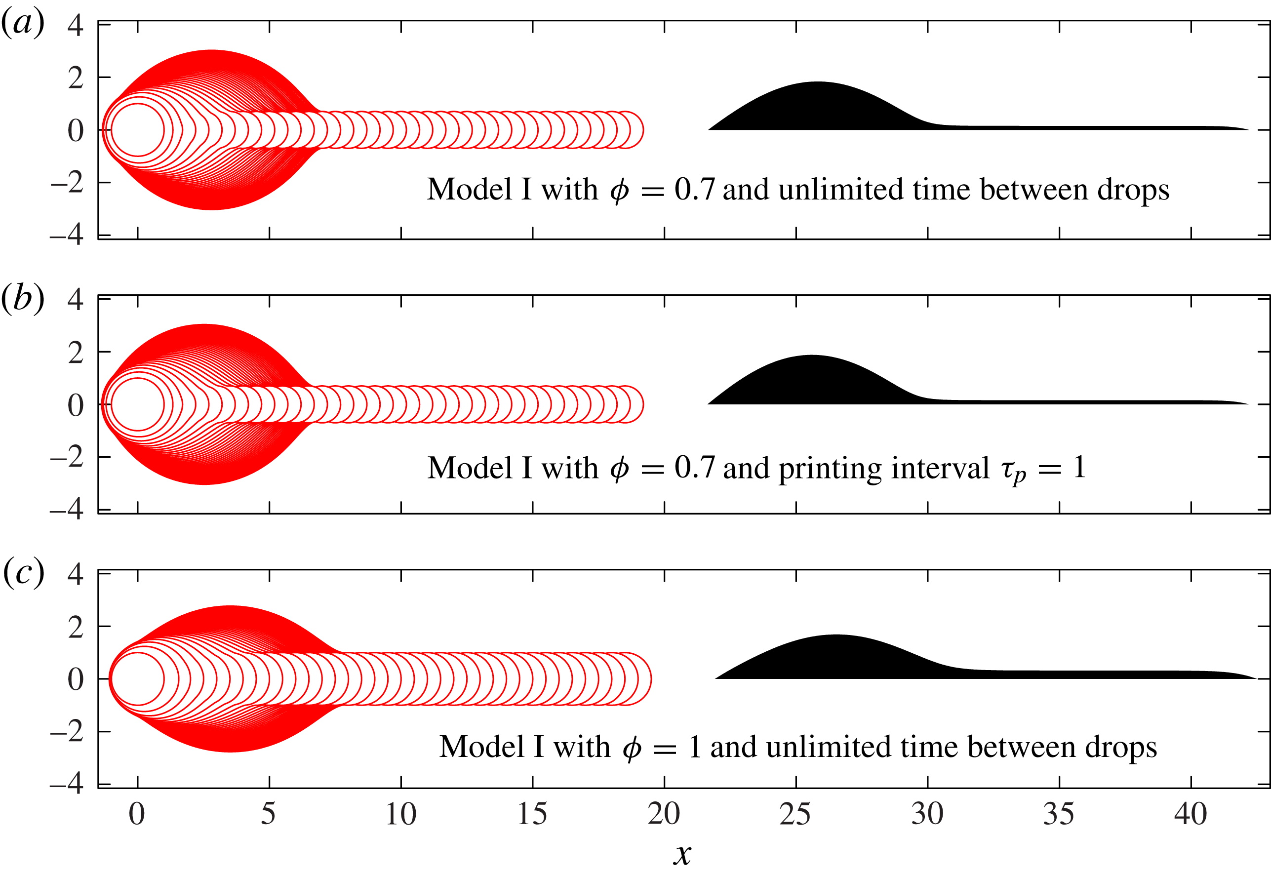
. Results with infinite
 ${\it\tau}_{p}$
and with
 ${\it\tau}_{p}=1$
, shown in figure 8(a,b), respectively, are virtually indistinguishable. In particular, the value of
 $U_{0}=0.3\ \text{m}\ \text{s}^{-1}\ \text{rad}^{-1}$
provided by the Cox–Voinov law leads to a relatively large dimensionless time
 ${\it\tau}_{p}=30$
between drops, which tends towards the infinite time results shown in figures 7 and 8(a). Furthermore, as shown in figure 8(c), increasing the value of
 ${\it\phi}$
from
 ${\it\phi}=0.7$
to
 ${\it\phi}=1.0$
leads to the formation of a wider rivulet because the pressure difference between bulk and drop is smaller and, hence, less fluid is driven into the bulk. Thus, the height difference between the primary bulge and the rivulet is reduced, but the qualitative features of the fluid footprint remain unchanged.
The effect on Model I results for
 ${\it\delta}=0.25$
of varying the time allowed between printed drops, and of setting
 ${\it\phi}=1$
rather than our standard value of
 ${\it\phi}=0.7$
. The dimensionless printing interval
 ${\it\tau}_{p}$
is defined as
 ${\it\tau}_{p}=T_{p}{\it\theta}_{A}U_{0}/R_{c}$
.
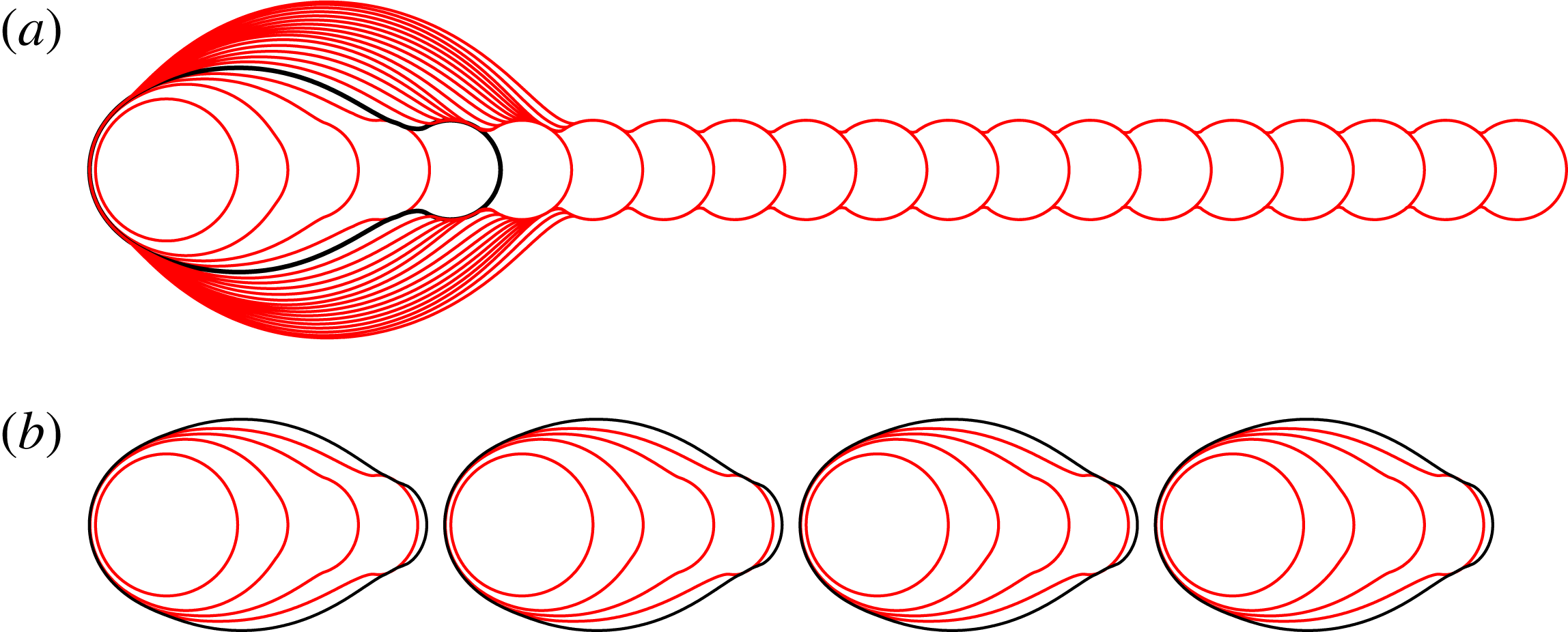
Our final investigation of Model I is to explore the effect of a non-zero receding contact angle
 ${\it\theta}_{R}$
, governed by the dimensionless parameter
 ${\it\epsilon}\equiv {\it\theta}_{R}/{\it\theta}_{A}$
. If
 ${\it\epsilon}=1$
, the only equilibrium configurations are circular islands. For
 ${\it\epsilon}=0$
, we obtain the non-receding system, in which a very long, very shallow rivulet can form. In figure 9, we show results for
 ${\it\epsilon}=0.5$
, calculated using the spreading law
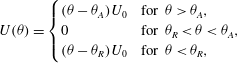 $$\begin{eqnarray}\displaystyle U({\it\theta})=\left\{\begin{array}{@{}ll@{}}({\it\theta}-{\it\theta}_{A})U_{0}\quad & \text{for }{\it\theta}>{\it\theta}_{A},\\ 0\quad & \text{for }{\it\theta}_{R}<{\it\theta}<{\it\theta}_{A},\\ ({\it\theta}-{\it\theta}_{R})U_{0}\quad & \text{for }{\it\theta}<{\it\theta}_{R},\end{array}\right. & & \displaystyle\end{eqnarray}$$
for the case
 ${\it\delta}=0.5$
,
 ${\it\phi}=0.7$
. We find that the deposited ink forms a sequence of identical, non-circular fluid islands, each consisting of exactly five fluid drops. These islands form because a non-zero receding angle allows very elongated rivulets to retract towards the primary head. Sufficient retraction prevents new drops from overlapping the existing fluid, resulting in the formation of a new line. If
 ${\it\delta}$
and
 ${\it\phi}$
are fixed and
 ${\it\epsilon}$
decreases, increasingly elongated rivulets can be sustained without retraction, so that the islands contain an increasing number of drops. It is possible that the retraction of elongated rivulets, rather than the breakup of a very long uniform line, may cause the regular disconnected islands of fluid observed at large drop spacing by Duineveld (Reference Duineveld2003) and also in our experiments, as shown in the second row of figure 2.
Model I simulations with and without a receding contact line. Here
 ${\it\delta}=0.5$
,
 ${\it\phi}=0.7$
, and there are 20 drops in each row. We define
 ${\it\epsilon}={\it\theta}_{R}/{\it\theta}_{A}$
, and show results for (a)
 ${\it\epsilon}=0$
and (b)
 ${\it\epsilon}=0.5$
. The shape of the contact line is exactly the same in both cases for the first three drops. The fourth contour shows small differences. The contact line after drop five is shown in black in each row; these differ significantly. In the case with
 ${\it\epsilon}=0.5$
, the extended rivulet has retracted sufficiently after the fifth drop to prevent overlap with the next printed drop. Instead, the next printed drop forms the start of a new line. Continuing to print equally spaced drops leads to an exactly repeated sequence of islands each containing five drops.
3.3. Model II: Viscosity regulates fluid redistribution within the footprint
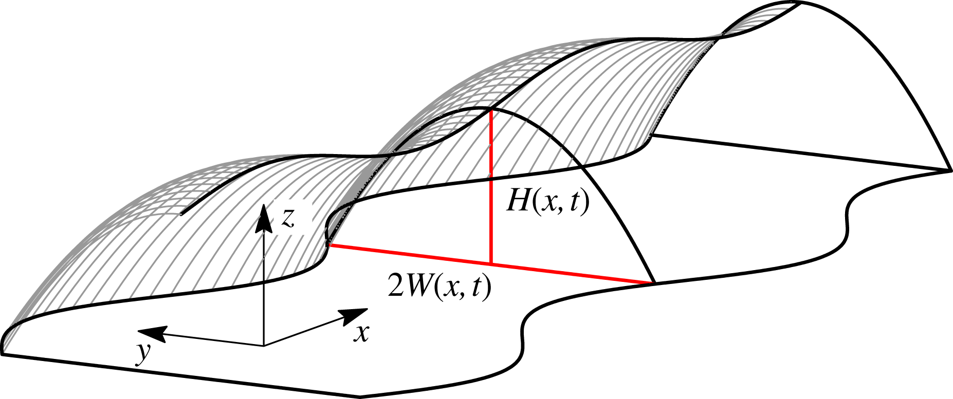
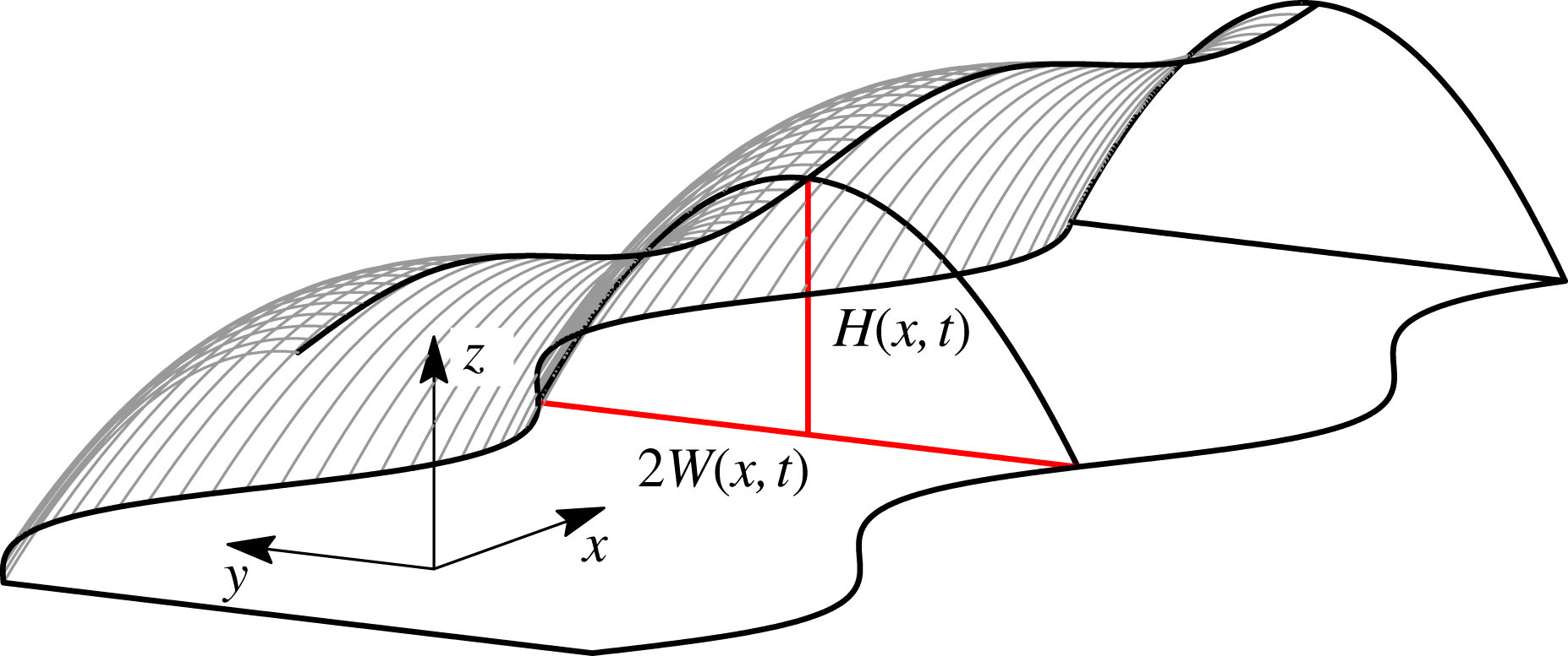
Secondary bulge formation requires viscous resistance to fluid redistribution within the footprint, which is the new effect incorporated in Model II. Our formulation uses a simplified description of the rivulet geometry, characterised by its width
 $W(x,t)$
and centreline height
 $H(x,t)$
, in order to avoid introducing additional slip mechanisms required for a full 2D viscous lubrication simulation, and to minimise computational cost. We use Cartesian coordinates, where the
 $x$
-axis is aligned with the direction of printing, the footprint lies in the
 $(x,y)$
plane and
 $z$
is directed out of the plane, as shown in figure 10. We will assume that the film is shallow and slowly varying, or equivalently that
 $L\gg W_{0}\gg H_{0}$
, where
 $L_{0}$
,
 $W_{0}$
and
 $H_{0}$
are typical lengthscales of the fluid island in the
 $x$
,
 $y$
and
 $z$
directions, respectively.
A 3D interface represented by the parabolic height profile (3.6), characterised by its width
 $W(x,t)$
and centreline height
 $H(x,t)$
.
Under the thin film assumptions (i.e.
 $H_{0}\ll W_{0}$
and
 $H_{0}\ll L$
), the evolution of the film height is governed by the free-surface version of the lubrication equations:
 $$\begin{eqnarray}\frac{\partial h}{\partial t}-\frac{1}{3{\it\mu}}\boldsymbol{{\rm\nabla}}\boldsymbol{\cdot }(h^{3}\boldsymbol{{\rm\nabla}}p)=0,\quad p=-{\it\sigma}{\rm\nabla}^{2}h,\end{eqnarray}$$
noting that the factor of three arises because we apply boundary conditions representing no slip on the solid substrate at
 $z=0$
, and no tangential stress on the free surface at
 $z=h$
.
We write the contact-line position as
 $y=\pm W(x,t)$
. If
 $W$
varies slowly with
 $x$
, the parameter
 ${\it\lambda}=W_{0}/L$
is small. Expanding (3.5) in powers of
 ${\it\lambda}$
, we find at leading order that any pressure gradients in the
 $y$
direction will be quickly driven to equilibrium. Pressure gradients in the
 $x$
direction decay over a timescale larger by a factor of
 ${\it\lambda}^{-2}$
. On this slow timescale, the pressure is effectively independent of
 $y$
, and the leading-order height profile is a solution to
 $h_{yyy}=0$
with boundary condition
 $h=0$
on
 $y=\pm W$
. We solve these equations to yield the parabolic profile
 $$\begin{eqnarray}h(x,y,t)=H(x,t)\left(1-\frac{y^{2}}{W(x,t)^{2}}\right).\end{eqnarray}$$
The fluid line is thus characterised by its width
 $W(x,t)$
and centreline height
 $H(x,t)$
. An example of a 3D free surface described by (3.6) is shown in figure 10.
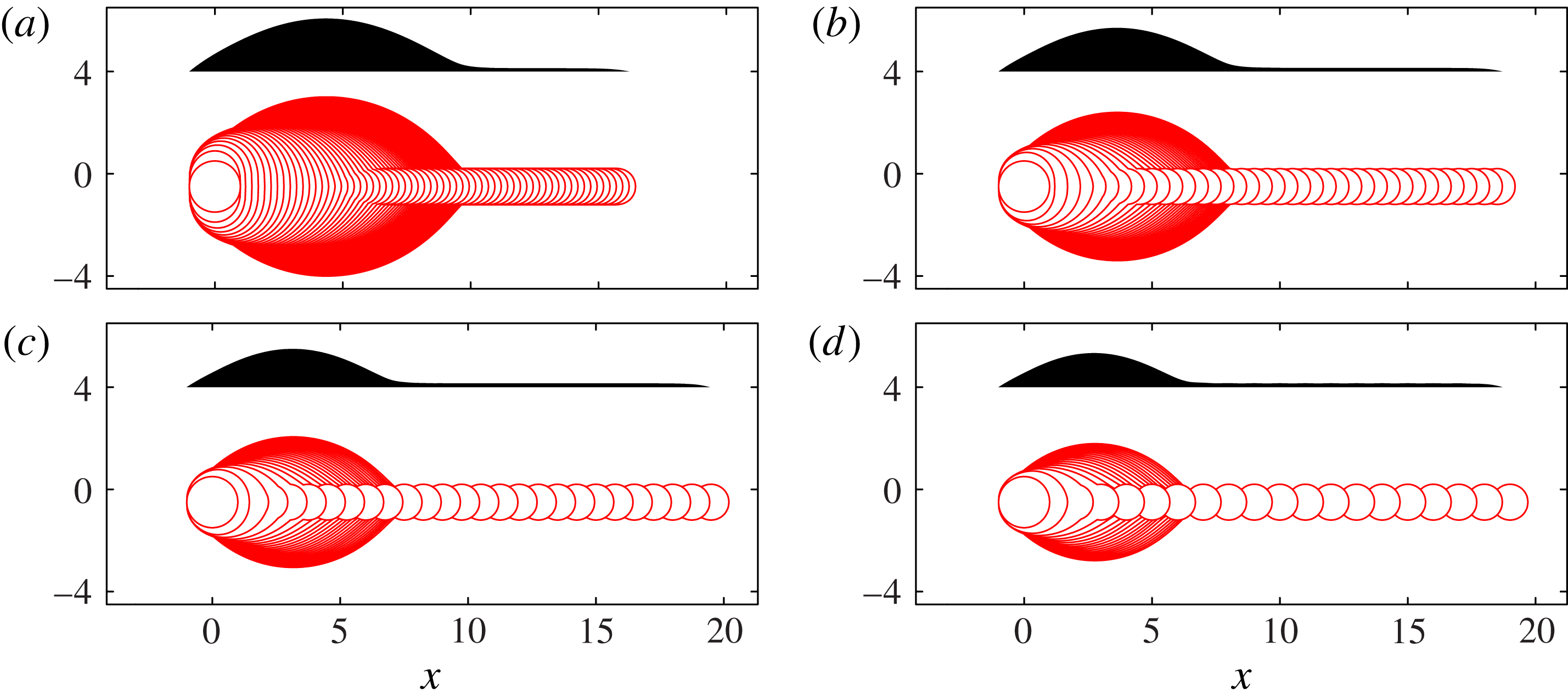
Model I results recalculated within the geometrical description of § 3.2, which exploits a slowly varying rivulet to describe the 3D geometry by 1D equations. The values of
 ${\it\delta}$
in (a–d) again match those in figure 3. These results should be compared with figure 7 for a less-restrictive geometrical description with the same physical mechanisms as here. Figure 13 uses the same geometrical description, but with the addition of viscous resistance to fluid motion in the
 $x$
-direction; we find that viscous resistance leads to secondary bulge development.
Any pressure gradients in the
 $x$
direction will drive a net flow resisted by viscosity. We obtain a one-dimensional (1D) viscous transport equation to describe this process by integrating (3.5) across a line of constant
 $x$
, thus relating the cross-sectional area
 $A$
and the net volume flux
 $Q$
:
 $$\begin{eqnarray}\frac{\partial A}{\partial t}+\frac{\partial Q}{\partial x}=0,\quad A\equiv \int _{-W}^{W}h\text{d}y,\quad Q\equiv -\frac{1}{3{\it\mu}}\int _{-W}^{W}h^{3}\frac{\partial p}{\partial x}\,\text{d}y.\end{eqnarray}$$
We now suppose that pressure is independent of
 $y$
,
 $p=P(x,t)$
, and use the parabolic height profile (3.6) to write
 $A$
and
 $Q$
in terms of
 $H$
and
 $W$
, which yields
 $$\begin{eqnarray}\frac{\partial }{\partial t}\left(HW\right)-\frac{\partial }{\partial x}\left(\frac{8}{35{\it\mu}}H^{3}W\frac{\partial P}{\partial x}\right)=0.\end{eqnarray}$$
In order to calculate
 $P(x,t)$
, we use the pressure along the fluid centreline:
 $$\begin{eqnarray}P(x,t)=-{\it\sigma}{\rm\nabla}^{2}h|_{y=0}={\it\sigma}\left(\frac{2H}{W^{2}}-H_{xx}\right).\end{eqnarray}$$
We will allow
 $W$
to evolve according to the same contact-line spreading scheme as used in Model I. In terms of
 $W$
, at
 $y=\pm W$
, we have
 $\boldsymbol{R}=(x,\pm W(x,t))$
and
 $\boldsymbol{n}=(-W_{x},\pm 1)/(1+W_{x}^{2})^{1/2}$
. We substitute these expressions for
 $\boldsymbol{R}$
and
 $\boldsymbol{n}$
, along with the height profile (3.6), into (3.3) to obtain
 $$\begin{eqnarray}\frac{W_{t}}{(1+W_{x}^{2})^{1/2}}=U({\it\theta})\quad \text{for }{\it\theta}=\frac{2H}{W}(1+W_{x}^{2})^{1/2}.\end{eqnarray}$$
We retain quasi-static contact-line dynamics as the spreading of
 $W$
is perpendicular to any pressure gradient, which would be along the length of the line. For simplicity, we do not allow spreading at the two ends of the domain, instead pinning
 $H=0$
and
 $W=0$
there. In order to allow uninhibited competition between drop arrival, viscous transport and contact-line spreading, we no longer wait for the contact line to come to rest before printing the next drop, but instead fix the printing time interval at
 $T_{p}=1/f$
.
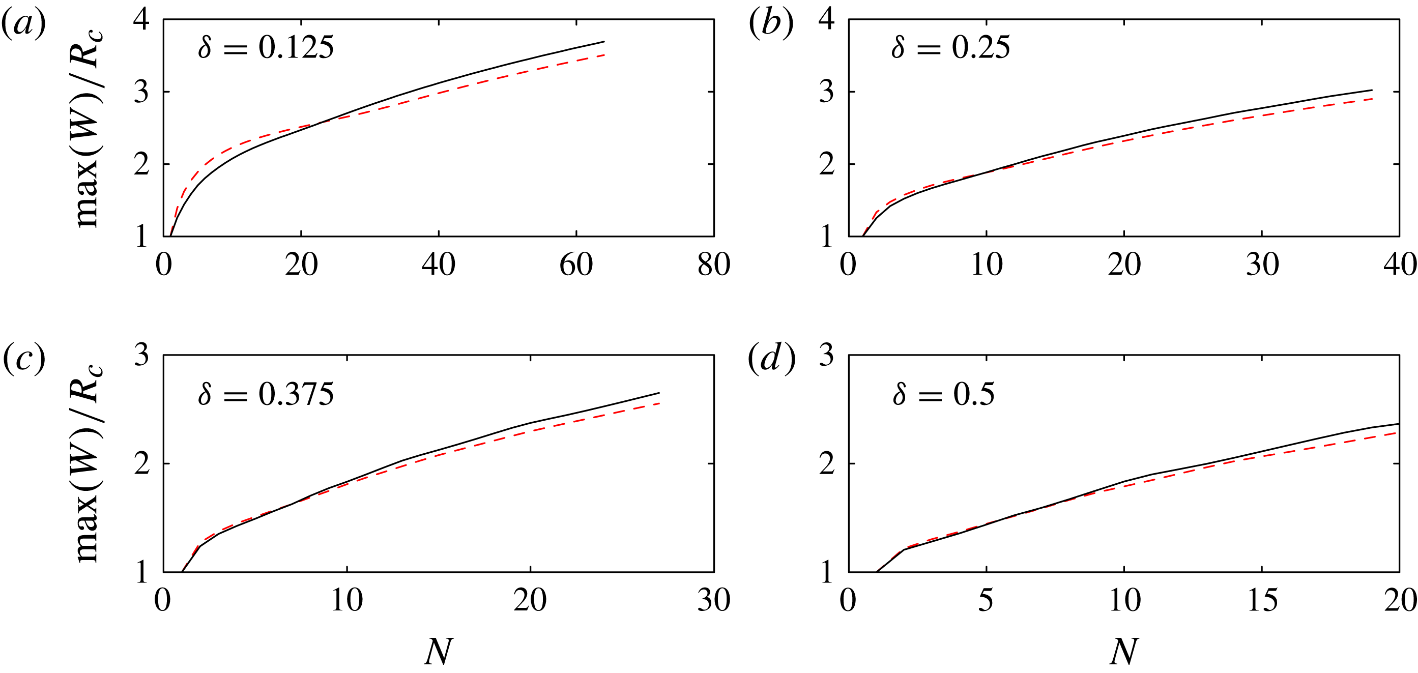
The predicted maximum bulge width for Model I, calculated according to the full 2D equations (solid line, full results shown in figure 7), and the 1D equations derived in § 3.3 (dashed line, full results shown in figure 11), with parameters in (a–d) matching figure 3. In both cases, we neglect viscous resistance, set
 ${\it\phi}=0.7$
, and allow sufficient time between successive drops for the contact line to come to rest.
The most important difference between Model II and a standard 1D lubrication model for fluid redistribution is the
 $2H/W^{2}$
term in (3.9), representing the curvature of the interface in the
 $y{-}z$
plane. Hernández-Sánchez et al. (Reference Hernández-Sánchez, Lubbers, Eddi and Snoeijer2012) used the standard 1D lubrication model to study flow in a connecting liquid bridge during coalescence of millimetre-sized droplets on a substrate, and found that the equations captured the correct similarity form. However, the
 $2H/W^{2}$
term is not negligible for slowly varying rivulets, as this term is typically much larger than
 $H_{xx}$
, and it supplies the only coupling between centreline height and contact line shape in the constant-pressure equilibrium state reached long after printing. The evolution equation (3.8) is also related to the equations for flow in a bounded rivulet on an inclined plane (Duffy & Moffatt Reference Duffy and Moffatt1995), although our system is driven by surface tension rather than gravity.
Both Model I and Model II involve descriptions of the 3D geometry of the air–fluid interface and its contact line. In Model I, we used 2D equations to describe the 3D system, with a contact line free to move in all directions. In Model II, we use 1D equations to describe the 3D system, and the contact line is pinned at the two end points of the fluid line. In order to clarify the effect of the different geometric descriptions, we recalculate Model I results using the 1D equations, but with the same physical ingredients as in § 3.2, so that the system evolves according to the spreading law (3.10), with spatially constant pressure computed according to (3.9), and the volume constraint calculated by integrating (3.6) over the length of the line. The recalculated Model I results are shown in figure 11, and a quantitative comparison of the bulge width as predicted by the two sets of equations is shown in figure 12. These results are in good agreement except that in our 1D description, we do not allow the end points of the domain to move and so the contact line can never spread behind the initial wetted region; this leads to some squashing of the first few drops in each line which widens the initial bulge. We note that the
 $(1+W_{x}^{2})^{1/2}$
terms in (3.10) were neglected by Duineveld (Reference Duineveld2003) in his analysis of bulge shapes. We find that retention of these terms leads to much better agreement with the fully 2D Model I results, particularly for the footprint shape of the primary bulge.
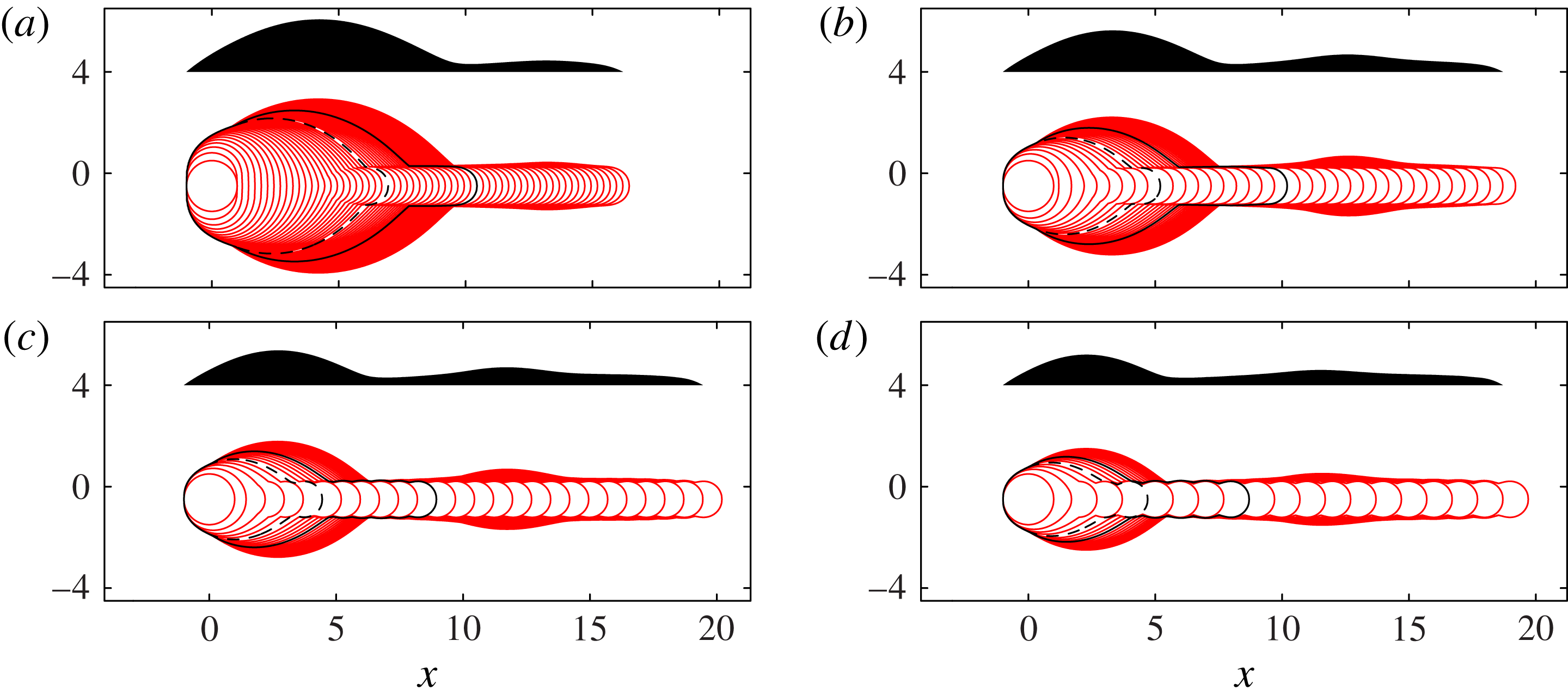
Figure 13 shows top- and side-view results from Model II, which includes viscous resistance to flow along the length of the rivulet. Comparing figures 11 and 13, we see that viscous resistance has very little effect on the contact-line shape for the first drops in each line, and does not affect the initial development of the primary bulge. However, in figure 13, a secondary bulge does eventually appear for large
 $N$
, and we find that the secondary bulge arises only in simulations with viscous resistance. The secondary bulge develops several drop lengths behind the rivulet tip, migrating to slightly larger
 $x$
as more drops are printed. The primary head continues to grow very slowly as the second bulge forms.
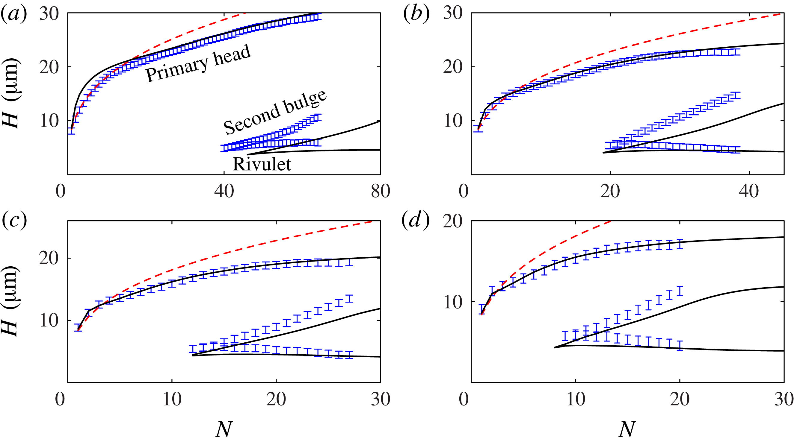
Drop-by-drop comparison of the experimentally observed and predicted side-view profiles, shown in figures 14 and 15, and also in the four supplementary movies, reveals that the numerical results for the full Model II, with
 ${\it\phi}=0.7$
and
 $U_{0}=0.01\ \text{m}\ \text{s}^{-1}\ \text{rad}^{-1}$
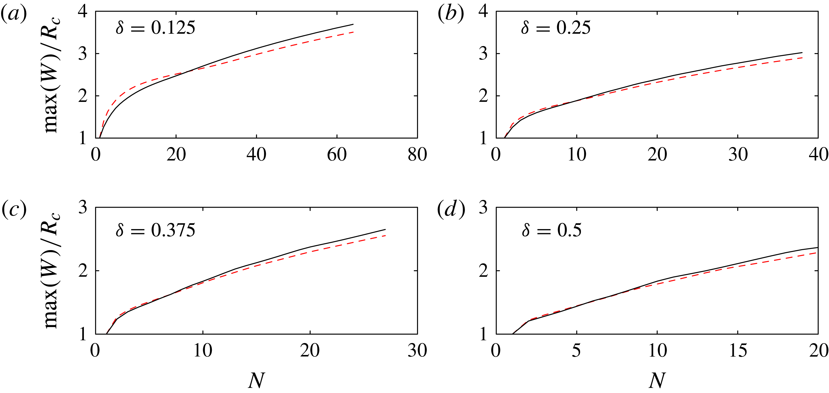
, are in good quantitative agreement with the experiments for both the primary head and secondary bulge. Figure 15 also includes results from a static calculation for the initial bulge height: a cube-root prediction obtained by gathering
 $N$
drops of volume
 $V_{0}$
into a spherical cap with contact angle
 ${\it\theta}_{A}=50^{\circ }$
. The Model II results are in better agreement with the experimental data than the static calculation except for small
 $N$
at the smallest drop separation, when the fixed end points leads to an artificially elevated drop in Model II.
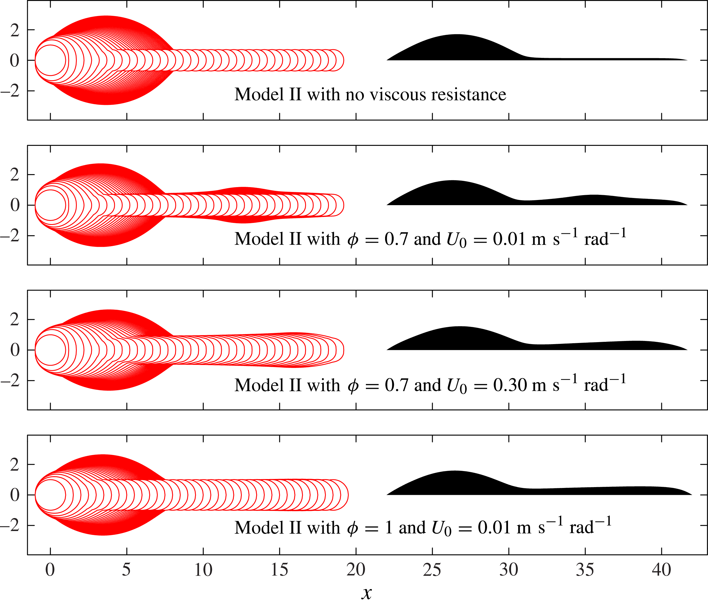
Superimposed contact-line positions (solid lines) and final side-view profile (shaded) for Model II, with parameters in (a–d) matching figure 3. Here
 ${\it\phi}=0.7$
and
 $U_{0}=0.01\ \text{m}\ \text{s}^{-1}\ \text{rad}^{-1}$
. These calculations include viscous resistance. As in figure 3, we indicate the contact-line position at
 $N_{1}$
(dashed black line), where the side profile is no longer convex and
 $N_{2}$
(solid black line), where the side profile first develops a second local maximum.
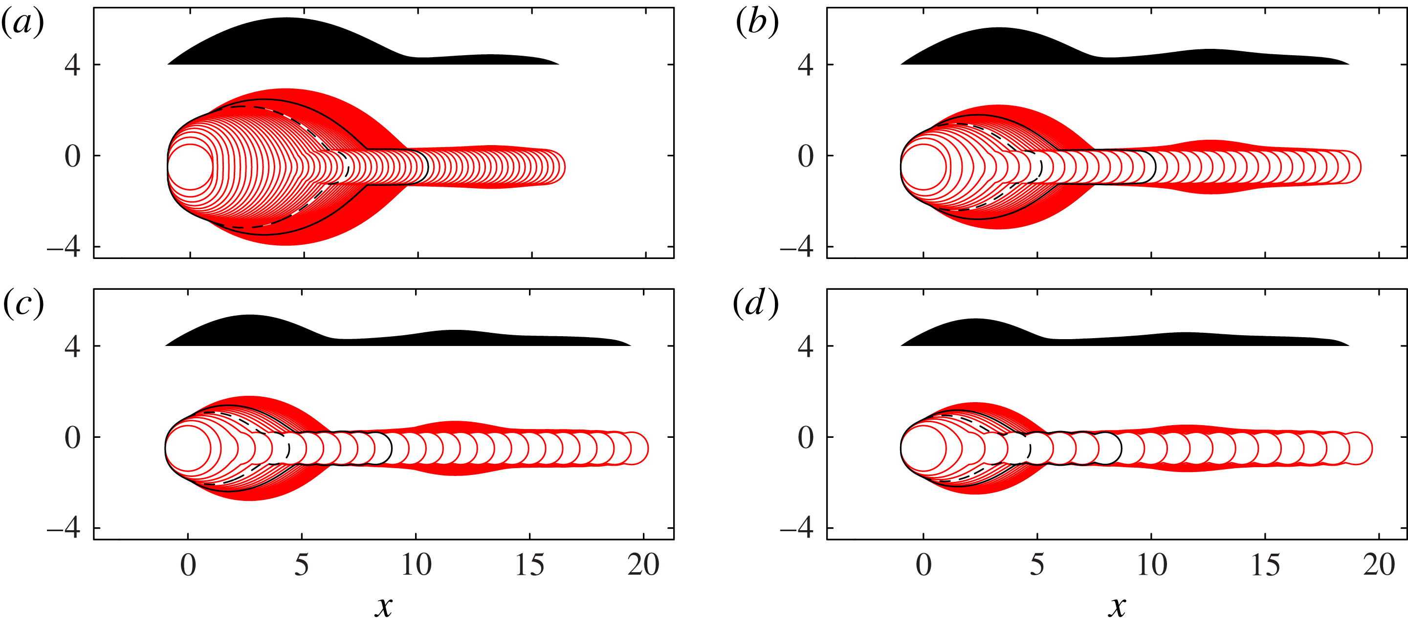
Comparison of top- and side-view Model I (from figure 7) and Model II (from figure 13) predictions to the side-view experimental results, after the final drop in each line is printed. A drop-by-drop comparison of Model II predictions and the side-view experimental results can be seen in the supplementary movies.

Maximum height of the primary head and second bulge, and minimum rivulet height, for experimental results from figure 3 (shown with error bars representing the height of a single pixel) and Model II results from figure 13 (solid lines). Parameters in (a–d) match figure 3. The (red online) dashed line shows a cube root height prediction for the primary bulge, based on arranging
 $N$
drops of volume
 $V_{0}$
into a spherical cap of angle
 ${\it\theta}_{A}=50^{\circ }$
.
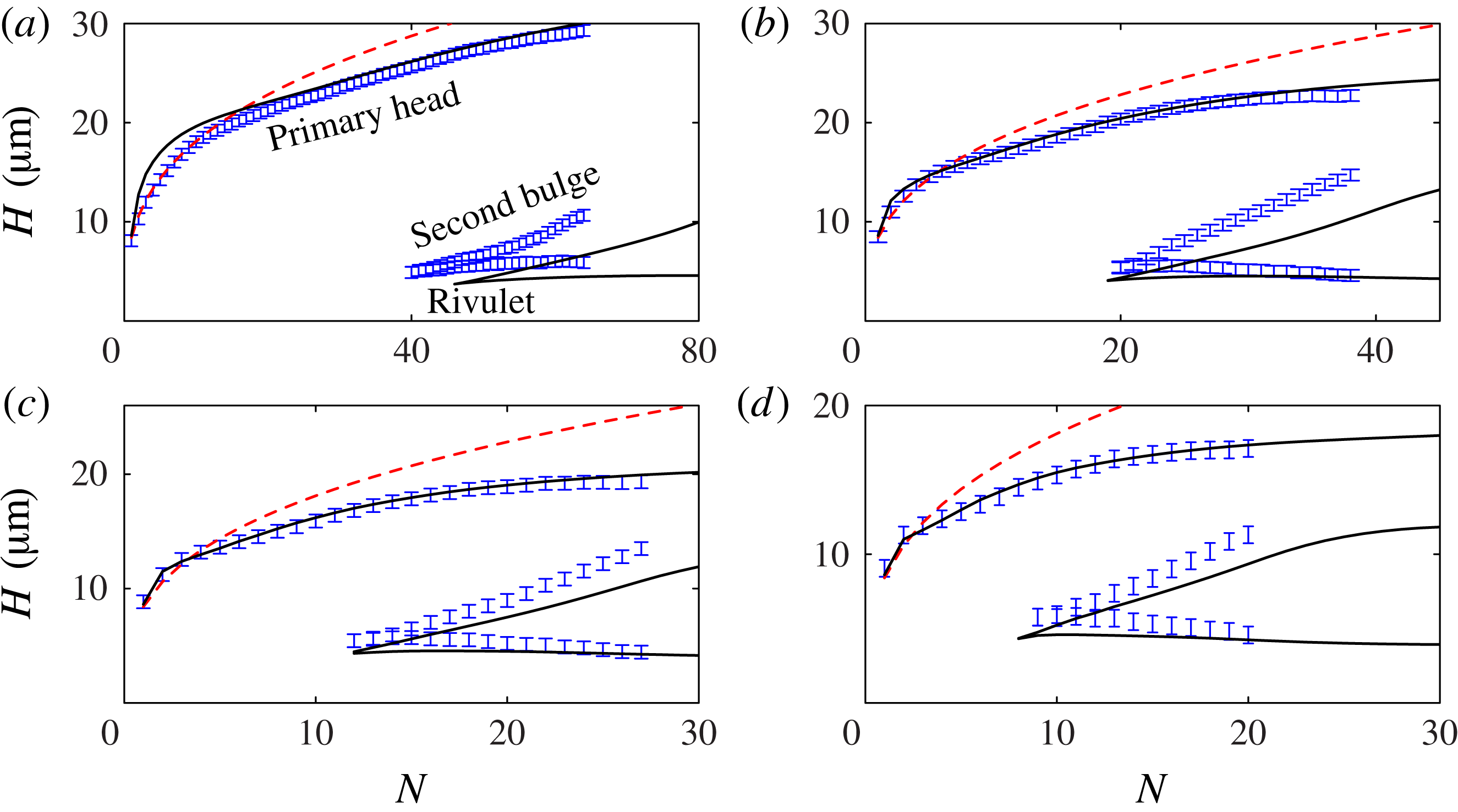
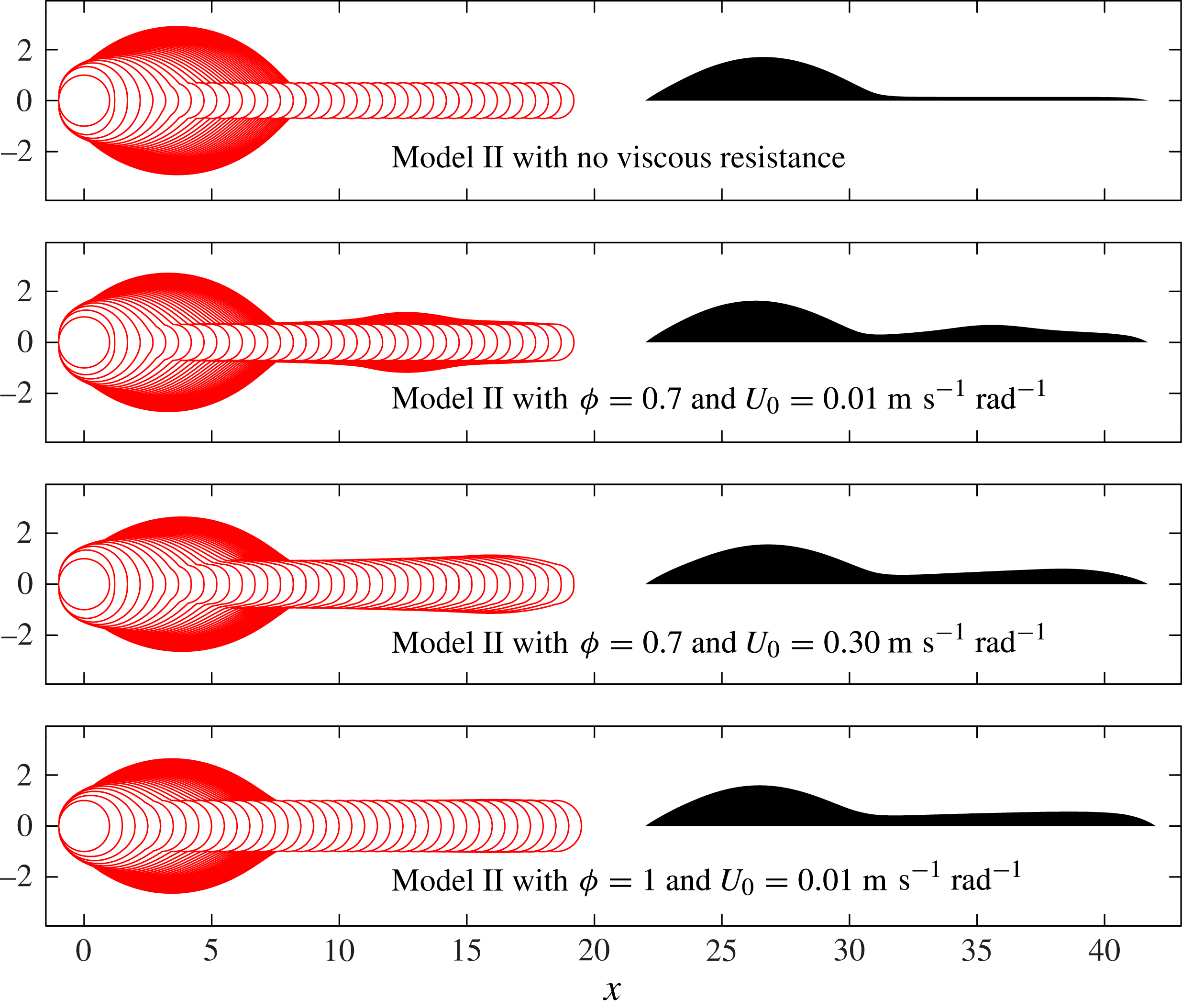
Figure 16 shows the effect of varying
 ${\it\phi}$
and
 $U_{0}$
on the Model II results. We find that bulge formation is not qualitatively affected by the spreading parameter
 ${\it\phi}$
, but decreasing
 ${\it\phi}$
reduces the wetted area, yields taller structures, and increases fluid mobility as a result of the increased contact angle. Figure 16 also shows Model II results for
 $U_{0}=0.3\ \text{m}\ \text{s}^{-1}\ \text{rad}^{-1}$
, which is the least well-established of the parameters in the model. This alternative value of
 $U_{0}$
is based on the Cox–Voinov law, and is 30 times larger than our experimentally measured value used for figure 13. However, for both values of
 $U_{0}$
with
 ${\it\phi}=0.7$
shown in figure 16, there is evidence of secondary bulge development, and so we conclude that the qualitative results are reasonably insensitive to
 $U_{0}$
, at least for the relatively short printed lines in our system.
A comparison of Model II results for
 ${\it\delta}=0.25$
with and without viscous effects, and also the effect of varying
 ${\it\phi}$
and
 $U_{0}$
. We find that viscous resistance causes fluid to accumulate in the rivulet, which enables possible formation of a secondary bulge. In all cases with viscous resistance presented here, there is a second local maximum in the height profile. Variations in
 ${\it\phi}$
and
 $U_{0}$
do not prevent fluid accumulating, but do affect the shape of the second bulge. A pictorial comparison of the Model II results with
 ${\it\phi}=0.7$
and
 $U_{0}=0.01\ \text{m}\ \text{s}^{-1}$
with the experimental results is shown in figure 14, and demonstrates good agreement for the shape of both the primary and secondary bulge with the experimental side views.
The parameters in Model II can be used to construct three timescales, corresponding to viscous resistance, contact line spreading, and the enforced printing interval
 $T_{p}=1.9\times 10^{-3}\ \text{s}$
. Contact line spreading is again characterised by
 $T_{c}=R_{c}/({\it\theta}_{A}U_{0})=2.1\times 10^{-3}\ \text{s}$
; the comparable values of
 $T_{p}$
and
 $T_{c}$
allow meaningful time for the contact line to spread before the next drop is deposited. Viscous resistance sets the timescale for fluid redistribution within the footprint, but depends strongly on the degree of elongation. If the rivulet varies in the axial direction over length
 $L$
, has typical height
 $H$
and width
 $W$
, we can use (3.8) and (3.9) to estimate the viscous timescale
 $T_{v}\sim {\rm\mu}L^{2}W^{2}/({\it\sigma}H^{3})$
. For a single drop with small contact angle, the appropriate lengthscales are
 $L\sim R_{c}$
,
 $W\sim R_{c}$
and
 $H\sim {\it\theta}_{A}R_{c}$
, and so the initial viscous timescale would be
 $T_{v}={\it\mu}R_{c}/({\it\sigma}{\it\theta}_{A}^{3})=4\times 10^{-6}\ \text{s}$
, which is much shorter than the timescale for contact-line spreading. However, after a large number of drops, Model I predicts that nearly all of the fluid is contained in the bulge, which is connected to a long shallow rivulet, of length
 $L=O({\it\delta}NR_{c})$
, height
 $H=O({\it\theta}_{A}R_{c}N^{-1/3})$
and width
 $W=O(R_{c})$
for large
 $N$
. This yields
 $T_{v}\sim {\it\mu}{\it\delta}^{2}N^{3}R_{c}/({\it\sigma}{\it\theta}_{A}^{3})$
, so that the viscous timescale increases strongly for large
 $N$
.
A simple estimate for the onset of secondary bulge formation could be obtained by setting
 $T_{v}$
equal to
 $T_{p}$
, so that the secondary bulge grows when fluid is deposited in the rivulet more quickly than it can be removed. According to this criterion, decreasing the fluid viscosity or allowing a greater time interval between printed drops would allow more fluid to reach the primary bulge, and thus increase the number of drops required for the onset of secondary bulge formation. However, this estimate neglects the continual evolution of the system and the sensitivities of contact-line motion.
4. Discussion
Our focus in § 3 has been on the development of simplified models that can quantitatively predict the development of relatively short ink-jet printed lines. These short lines are typically dominated by a large primary head which develops due to the merging of the first drops in each line. We have presented and analysed two models, which are both based on separation of scales between various processes in the printing dynamics.
In Model I, the system is dominated by a spreading law with hysteresis coupled to a fluid interface arranged at constant curvature. This quasi-static spreading is valid if the fluid within the ink footprint is redistributed to eliminate pressure variations at a rate much faster than the contact-line motion. We also assumed that the arrival rate of individual droplets is much slower than the contact-line speed. Based on our spreading law and the printing frequency, the drops have an
 $O(1)$
dimensionless time to spread between the arrival of each drop; this successive spreading is able to set a strong asymmetry between the first and last drops to arrive.
In Model II, we relax the quasi-static assumption in one direction only, which is needed to understand fluid motion along the length of the rivulet. Model II has three competing timescales, due to contact-line motion, fluid redistribution along the length of the rivulet, and the fixed frequency of droplet deposition. These three timescales may interact in complex ways, especially for very long lines. We note that previous models (Schiaffino & Sonin Reference Schiaffino and Sonin1997; Duineveld Reference Duineveld2003; Stringer & Derby Reference Stringer and Derby2010) do not assign a timescale to contact-line spreading, and so feature only one dimensionless timescale.
In our analysis, impact contributes only an initial condition for subsequent slow spreading of fluid on the substrate. In our calculations, all of the effects of impact are lumped into a single parameter
 ${\it\phi}$
, which defines the distance an impacting drop is spread across before appreciable interaction occurs with any fluid that has already been deposited. In principle, impact could result in a fully three-dimensional flow field with inertia, and so it is not obvious that impact characteristics can be crudely lumped in this way. However, for spreading in thin films, any fluid motion is in close proximity to a rigid substrate, and so we expect inertia to dissipate rapidly.
In both models, we have used small angle assumptions to characterise the geometry. Small angles allow us to use thin-film approximations for the interface curvature, the relationship between contact angle and the interface height profile, the cross-sectional area, and the fluid flux along the length of the rivulet. For larger contact angles, these expressions would be more complicated, e.g. each parabolic cross-section in figure 10 would become a circular arc, but could nonetheless be included within the general model framework.
The substrate in our experiments has a very low receding contact angle, and we have typically assumed that this angle is zero in our simulations. In figure 9, we simulated line development in the case of a non-zero receding angle. We find that a non-zero receding angle allows elongated rivulets to retract towards the primary head, and can thus prevent connection with the next printed drop. As a result, the sequence of printed droplets leads to a sequence of fluid islands, each containing a whole number of drops. Simulation of retracting rivulets in Model II would require modification of the mathematical formulation to allow the end points of the rivulet to move, and would also require a rupture criterion if the ink line were to ever break up into islands.
In general, we expect our models to work well for microscale systems with well-separated timescales between the dissipation of impact inertia, fluid redistribution within the footprint (at least for a circular drop), contact-line motion and drop arrival intervals. Other effects that are likely to become significant include evaporation, coffee-ring effects, non-Newtonian behaviour due to suspended particles, surface tension or viscosity variation, and gravity for millimetric drops. All of these effects could be included within our model framework allowing quantification of the relative importance of each on comparison with experimental data.
For our system, it appears that no choice of
 ${\it\delta}$
is able to yield a liquid line that is uniform along its whole length. The first drops will always merge together to form a primary bulge that sucks fluid from later drops, and so the base state is never a uniform line of static fluid. At very large drop spacing, the flow towards the bulge may be weak, but then the line becomes increasingly prone to scalloping and disconnections. We anticipate two circumstances when a uniform line might be achieved. First, if we discount the primary bulge, allowing a very long time between deposition of individual drops will drive the system towards Model I results, with a very shallow, but essentially uniform rivulet. The second approach is to use a very viscous fluid, so that there is no spreading between drops and no movement along the rivulet, allowing the whole line to spread uniformly.
5. Conclusion
We have used new experimental observations to develop novel models that quantitatively predict the evolution of post-impact line morphology during the printing of offset droplets. Model I demonstrates that the (previously unexplained) primary head forms as a consequence of contact angle hysteresis when surface tension is strong enough that spreading can occur between droplet arrivals. Once formed, the primary head fundamentally alters later dynamics because the relatively low pressure within the head drives a net internal fluid flow back towards the start of the line. The development of secondary bulges requires the inclusion of viscous resistance, which slows the capillary flow until the fluid cannot all be transported away from the rivulet tip before the next drop arrives.
Even for the purely fluid dynamical interactions described here, both experiments and models indicate rich morphology for longer printed lines. Moreover, the models can be easily extended to include additional physical effects such as evaporation, substrate topography or wettability variations, and adapted to account for larger contact angles or other forms of spreading law. Due to the simplicity, accuracy and flexibility of our approach, we are confident that closely related models can be developed to provide physical insight and predictive power for a wide range of significantly more complex systems.
Acknowledgements
We acknowledge funding from EPSRC (grant EP/H011579/1 and Pathway to Impact scheme). We are very grateful to Cambridge Display Technology Limited for the use of their printing facilities.
Supplementary movies
Supplementary movies are available at http://dx.doi.org/10.1017/jfm.2014.621.