1. Introduction

Philosophers, statisticians, and computer scientists, at least those who have abandoned the goal of producing a reductive account of causation, have come to largely agree on how to represent qualitative causal claims and how to connect such claims to statistical evidence through probabilistic independence and dependence (Glymour and Cooper Reference Glymour and Cooper1999; Pearl Reference Pearl2000; Spirtes et al. Reference Spirtes, Glymour and Scheines2000; Woodward Reference Woodward2003).Footnote ¹ Included in this scheme is a method for representing experimental interventions, and for clarifying what sorts of assumptions we must make about interventions in order to consider them ‘ideal’. With this apparatus, it is easy to show that if we have ideally intervened experimentally upon (X), then an association between X and Y entails that X is a cause of Y. Inferring that one variable is a cause of another is what I call ‘causal inference’.

With this apparatus, Spirtes et al. (Reference Spirtes, Glymour and Scheines2000), Pearl (Reference Pearl1988, Reference Pearl2000) and others have developed algorithms for determining the set of causal structures that are consistent with the independence relations assumed to hold over a set of measured variables in a non-experimental, or observational study, even causal structures that include latent, or unmeasured variables. In some instances all the causal structures in an equivalence class agree on some subset of the causal relations, and in some cases they all agree that one variable X is a cause or direct cause of another Y. In these cases we can, using basically the same assumptions as are made in experimental studies, infer that X is a cause of Y.

Although we have no general characterization of the conditions under which a causal inference to $X\rightarrow Y$ can be made in observational studies, it turns out that when the inference is possible it is often driven by the existence of what I call a detectible instrumental variable that stands in the same relationship to X and Y in the observational study as does the ideal intervention on X in the experimental study. In what follows, I briefly sketch the key ideas behind the representational system, I show how an experimental causal inference works in this system, how the typical observational causal inference works involving detectible instrumental variables, and the parallel between detectible instrumental variables and experimental interventions.

2. Representing Causation

2.1. Causal Graphs, Probability Distributions, and the Causal Markov Axiom

Recently from computer science, but as far back as Sewall Wright in the early twentieth century (Wright Reference Wright1934), the fundamental representational device for causal systems is the directed graph. A directed graph is simply a collection of vertices and directed edges over pairs of these vertices. In a directed graph interpreted as a causal graph, each directed edge (or arrow) from one vertex X to another Y is taken to assert that X is a direct cause of Y relative to the set of vertices in the graph. For example, Figure 1 represents a graph $\mathbf{G}=\langle \mathbf{V},\,\mathbf{E}\rangle $, with vertices V = {Exposure, Infection, Symptoms}, and edges E = {〈Exposure, Infection〉, 〈Infection, Symptoms〉}. We further assume that the vertices in such a graph can be interpreted as random variables with some probability distribution P, and that causal processes situated in some definite background context generate probability distributions over these variables.

Figure 1.

Causal graph.

A causal graph is assumed to be representationally complete in the following sense: if two variables in the graph are effects of a common cause C, then C is included in the graph. This does not require us to include all the causes of a variable in the graph, it only requires that we include all the common causes. To be clear, this is a representational assumption, not one concerning which variables we will measure when the goal is inference. The key assumption connecting causal graphs to probability distributions is an axiom that constrains the set of probability distributions that a given causal graph can generate (Spirtes et al. Reference Spirtes, Glymour and Scheines2000):

Causal Markov Axiom. In any probability distribution P generated by a given causal graph G, each variable X is probabilistically independent of the set Y consisting of all variables that are not effects of X, conditional on the direct causes of X. That is, ∀ $X\in \mathbf{G}$, X⌋ ⌊ Non-effects of X | Direct Causes of X, in P.

This entails, for example, that Exposure is independent of Symptoms conditional on Infection in any probability distribution that the causal graph in Figure 1 can generate. In acyclic causal graphs, the Causal Markov Axiom is equivalent to a graphical relation called d-separation (Pearl Reference Pearl1988). If X and Y are d-separated by Z, then the Causal Markov Axiom entails that X and Y are independent conditional on Z.

2.2. Interventions

To model experimental interventions on a causal system, we add a new variable representing the intervention, connect it to the graph in a particular way, and make an assumption about how ideal interventions change the causal graph (Spirtes et. al Reference Spirtes, Glymour and Scheines2000; Pearl Reference Pearl2000). For simplicity we restrict interventions to act only on one variable at a time. Let an intervention on X be called I _X, and model this by adding I _X to the graph as a direct cause of only X, and the effect of no variable. For example, to model an experimental intervention on Infection in the causal graph in Figure 1, we build the graph in Figure 2.

Figure 2.

Modeling an intervention.

Modeling an intervention as a direct cause makes explicit the fact that this account of causation does not attempt to reduce causation to intervention. It goes to the other extreme, it reduces intervention to the idea of a direct cause. Direct cause is left undefined, but connected to probability through the Causal Markov Axiom.

Finally, we say an intervention is ‘ideal’ if it totally determines the probability distribution of its target. For example, a medical trial assessing the effect of St. John's Wort on depression might assign either of two treatments: St. John's Wort or placebo, by flipping a fair coin to randomly assign subjects to one of these two treatments. This intervention is ideal if the coin flip totally determines the treatment, leaving no influence from the subject's disposition to take alternative medicines, etc.

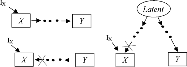
If I _X is an ideal intervention on X, then we eliminate, or ‘x-out’ any arrows in the original causal graph that point into X (Figure 3). This represents the idea that our ideal intervention has taken over X's probability distribution, overwriting any influence its direct causes might have had prior to our intervention. In contrast, we do not x-out arrows coming out of X. So ideal interventions on X annihilate the relationship between X and its direct causes, but leave intact the relationship between X and its direct effects.Footnote ²

Figure 3.

Modeling an ideal intervention.

3. Causal Inference in Experimental Studies

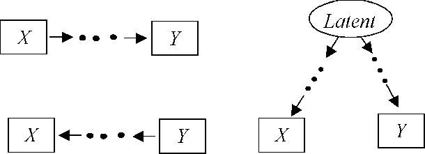
The problem of causal inference from association is underdetermination. If two variables X and Y are associated in a non-experimental study, then many different causal graphs can explain the association. In general, three kinds of causal connectionFootnote ³ (Figure 4) can produce an association (probabilistic dependence) between two variables X and Y:

1. 1. A pathFootnote ⁴ from X to Y

2. 2. A path from Y to X

3. 3. A pair of paths, one from some third variable C (possibly latent) to X and one from C to Y.

Figure 4.

Causal connections which explain an association between X and Y.

Consider the same problem after an ideal intervention on X, however. The intervention eliminates the influence of all the direct causes of X in the original graph, thus all causal connections save paths from X to Y are destroyed (Figure 5).

Figure 5.

Causal connections after an ideal intervention on X.

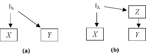
The result is incredibly simple, but incredibly powerful. If X and Y are associated after an ideal intervention on X, then X is a cause of Y. Further, the quantitative degree of association can be used to estimate the size of the effect of X on Y (Pearl Reference Pearl2000). The key to this type of simple experimental inference is that the intervention is: (i) a direct cause of X, (ii) not adjacent to Y, and (iii) ideal. Consider why it is desirable that it satisfy these conditions. First, if the intervention is a direct cause of X, but also of Y or some other cause of Y,Footnote ⁵ then X and Y will be associated in virtue of the intervention, not in virtue of the effect of X on Y (Figure 6). It is possible to handle the second form of fat-hand intervention (Figure 6b) by looking not just at whether X and Y are associated but also at whether X and Y are associated conditional on Z. The first type of fat-hand intervention (Figure 6a), in which I _X is a direct cause of Y is fatal to causal inference.

Figure 6.

Fat-hand interventions.

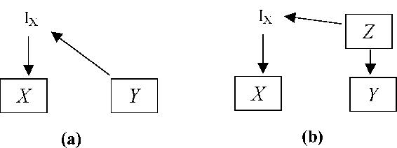
Similarly, the intervention must itself not be an effect of any other variable, a problem I will call treatment-bias (Figure 7). Again, in such cases X and Y would be associated after an intervention, but not because of an effect of X on Y. Again, we could handle the second form of treatment-bias (Figure 7b) by conditioning on Z, but the first form (Figure 7a) is fatal.

Figure 7.

Treatment-bias interventions.

Generally then, an intervention on X can be fat-hand or treatment-biased without making causal inference impossible, but I _X cannot be adjacent Footnote ⁶ to Y in the causal graph. Need the intervention be ideal? Is causal inference still possible in cases in which the intervention on X does not fully determine X's probability distribution and thereby x-out the influence of all other direct causes on X? For the argument as I have sketched it above, clearly yes, but in general the answer is no.

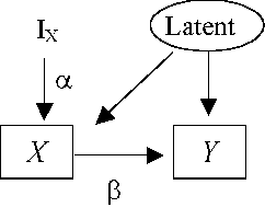
In cases where we know something about the parametric form of the dependence of effects on their causes, for example linear structural equation models (Bollen Reference Bollen1989), interventions need not be ideal. In linear structural equation models each effect is a linear combination of its direct causes plus Gaussian noise, and in certain such models instrumental variable estimators (Bowden and Turkington Reference Bowden and Turkington1984) can be used to estimate the strength of causal influence even in the presence of latent common causes. In Figure 8, for example, I _X is an instrumental variable for $X\rightarrow Y$, and the quantity $\rho _{IX,Y\,}/ \rho _{IX,X}=\alpha \beta / \alpha =\beta $ is a consistent estimator of the effect of X on Y, even though X and Y are confounded by a latent common cause. If I _X is an intervention, but not an ideal intervention, as in Figure 8, and the dependencies are linear, then the instrumental variable estimator can be used to do causal inference; we simply statistically test whether $\beta =0$. Whether or not the instrumental variable Z is an intervention, (i) Z must be adjacent to X but not an effect of X,Footnote ⁷ and (ii) Z may not be adjacent to Y.

Figure 8.

Instrumental variable I _X.

To summarize, in experimental settings causal inferences concerning whether X is a cause of Y are driven by interventions on X which are: (i) direct causes of X, (ii) not adjacent to Y, and (iii) ideal (they totally determine the probability of X).

4. Causal Inference in Non-experimental Studies

In non-experimental studies, we have no intervention variable with known relationships to the variables under study. We have only a set of measured variables governed by some causal structure that we assume satisfies the Causal Markov Axiom, but which might include unmeasured common causes of the variables we have measured. To set aside statistical difficulties, we will assume that we can determine which probabilistic independence relations hold over the measured variables with perfect reliability. Finally, we will assume that the probability distribution P is FaithfulFootnote ⁸ to the causal graph (Spirtes et al Reference Spirtes, Glymour and Scheines2000). That is, we assume that all independence relations that hold in P are entailed by the Causal Markov Axiom, thereby ruling out independence relations holding in P in virtue of particular settings for the probabilities in P.

In this setting, the underdetermination of causation can be characterized with an equivalence class of causal graphs, each member of which is a causal graph that entails all and only those independence relations observed to hold in some distribution P_O over the set of observed variables O. As you would expect, when we allow the equivalence class to include graphs that have unobserved common causes, that is, variables not in O, then the class is infinite. Spirtes and Richardson (Reference Spirtes and Richardson1996) describe a graphical object called a Partial Ancestral Graph or PAG, to compactly represent equivalence classes that include latent common causes.

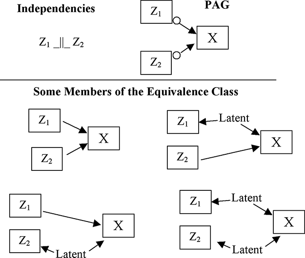
Fortunately, it is sometimes the case that all members of the equivalence class represented by a PAG share features of a causal relationship between two variables in O. For example, if we have measured three variables, Z ₁, Z ₂, and X, and find Z ₁ and Z ₂ to be unconditionally independent, then the PAG and some of the members of the equivalence class it represents are pictured in Figure 9. Even though X is associated with both Z ₁ and Z ₂, in no member of this equivalence class is X a cause of either Z ₁ or Z ₂. We can't, from three variables and no extra background knowledge make a positive causal inference, but we can make two negative ones: X is not a cause of Z ₁ nor is it a cause of Z ₂. With four variables we can actually make a positive causal inference. Adding Y, and assuming that Y is unconditionally associated with all the other variables but independent of Z ₁ and Z ₂ conditional on X, the PAG in Figure 10 represents the set of causal graphs that entail all and only these independencies. In every member of the equivalence class represented by the PAG in Figure 10, X is a cause of Y, and in no member of the equivalence class is there a latent common cause of X and Y, exactly the same conclusion we can reach by finding an association between X and Y in an experimental study in which we have ideally intervened upon X.

Figure 9.

Equivalence class.

Figure 10.

PAG that gives a causal inference.

The FCI algorithm (Spirtes et al Reference Spirtes, Glymour and Scheines2000) computes PAGs from given independencies, assuming the Causal Markov Axiom, Faithfulness, and that there is a graph that generated the independencies given. By examining one set of conditions required by the algorithm in order to determine that (i) X is cause of Y and (ii) there is no latent common cause of X and Y in every member of the equivalence class, I will try to illuminate the similarity between causal inference in experimental and non-experimental settings.

The FCI algorithm proceeds in two stages. In the first it identifies the adjacencies in the PAG, and in the second it orients any of these adjacencies it can. Any pair of variables that are not adjacent after the adjacency phase are not adjacent in any causal graph in the final equivalence class (Spirtes et al. Reference Spirtes, Glymour and Scheines2000). In a PAG, an unoriented adjacency is represented as Ao-oB. The possible orientations and what they represent about the members of the equivalence class are:

• • A o→ B means that B is not a cause of A in any member of the class, but either A is a cause of B or they have a latent common cause.

• • A ← → B means that A and B have a latent common cause in every member of the class.

• • A → B means that A is a cause of B with no latent common cause in every member, and

• • A o- $\underline{\mathrm{o}\,B\mathrm{o}\,}$-o C means that either (i) B is a cause of A and there is no latent common cause of A and B, or (ii) B a cause of C with no latent common cause.

In the orientation phase, the algorithm looks for triples A, B, C such that A and B are adjacent, B and C are adjacent, but A and C are not adjacent, i.e., A o-o B o-o C. If B is included in the set that made A and C independent,Footnote ⁹ then we orient this triple as a ‘non-collider’ at B: A o- $\underline{\mathrm{o}\,B\mathrm{o}\,}$-o C, else we orient the triple as a ‘collider’ at B: A o→ B ←o C. We call this orientation step the ‘collider rule’.

After going through all the triples and orienting them with the collider rule, we go through them again, this time looking for triples in which B was oriented as a non-collider from the triple A, B, C, but as collider from a triple A, B, D, that is Figure 11. We can then combine these orientations to fully orient the B o-o C adjacency as B → C, which is the only way to orient B o-o C in order to avoid making B a collider in the A, B, C triple. We call this the ‘away-from-collider rule’.Footnote ¹⁰

Figure 11.

Consider a concrete empirical case to illustrate. Sewall and Shah (Reference Sewall and Shah1968) collected data on over 10,000 Wisconsin high school seniors in order to study the relationship between parental encouragement (PE) and college plans (CP). They also measured socio-economic status (SES), Sex, and IQ. For simplicity I omit SES. The independence relations that hold statistically among PE, CP, Sex, and IQ are: Sex ⌋ ⌊ IQ, Sex ⌋ ⌊ CP|PE. After the adjacency phase of FCI, we have Figure 12. There are two triples that satisfy the requirements for orientation: (1) Sex o-o PE o-o IQ, and (2) Sex o-o PE o-o CP. In (1), we can orient PE as a collider,Footnote ¹¹ and in (2), we can orient PE as a non-collider.Footnote ¹² So after applying the collider rule we have the orientation in Figure 13. Going back through these two triples, we can apply the away-from-collider rule to the Sex, PE, CP triple, giving us a PAGFootnote ¹³ in which parental encouragement is an unconfounded cause of college plans (Figure 14).

Figure 12.

After adjacency phase.

Figure 13.

After applying the collider rule.

Figure 14.

PAG for college plans

5. The Similarities

Consider the inference to $X\rightarrow Y$ in a non-experimental setting with the away-from-collider rule. We need a triple $Z\,\mathrm{o}\,\underline{\rightarrow X\mathrm{o}\,}- \mathrm{o}\,\,Y$. Besides knowing that X and Y are adjacent,Footnote ¹⁴ this construction involves a detectible instrument Z that is: (i) adjacent to X but not an effect of X, and (ii) not adjacent to Y.

These conditions match precisely with those required of an instrumental variable as used commonly in econometrics (see Section 3 above), and they also match quite closely to the two conditions I specified for experimental studies, which I repeat here. Interventions I _X on X should at a minimum: (i) be direct causes of X, and (ii) not be adjacent to Y.

A variable V that satisfies the first condition will also satisfy the first condition for a detectible instrument Z, but structurally it is not necessary for V to directly cause X. It is enough that the adjacency between V and X be into X, that is, either V is a direct cause of X or there is a latent common cause of V and X. By intervening on X with I _X, we ensure that the adjacency between I _X and X is into X, but for the causal inference it is not strictly necessary.

I use the word ‘detectible’ to highlight the fact that, in a non-experimental study, the issue is finding a variable that detectibly satisfies the same basic conditions that we believe are satisfied in an experimental study. For example, in the case study involving college plans and parental encouragement above, we managed to detect that the adjacency between Sex and PE was into PE because Sex and IQ are independent, thus giving us a collider oriented triple: Sex o→ PE ←o IQ.

Suppose, however, that Sewall and Shah had not thought to measure IQ. Just measuring Sex, PE, and CP, and finding only that Sex ⌋ ⌊ CP|PE, we would have the following PAG: Sex o-o PE o-o CP, which does not support a causal inference between PE and CP. Why? Because we do not know that the Sex o-o PE adjacency is into PE. If, however, we add the perfectly plausible background knowledge that parental encouragement cannot be a cause of one's gender, then the variable Sex would satisfy the conditions for a detectible instrument: Sex is adjacent to PE but not an effect of PE (Sex o→ PE), and Sex is not adjacent to CP. In that case would have a detectible instrument and could, from the Causal Markov Axiom and Faithfulness assumptions, infer that parental encouragement is indeed a cause of college plans with no latent common cause between them.

The parallels between these forms of experimental and non-experimental inference are not complete, nor are they necessary. They do suggest, however, that faced with a causal question that does not permit, for ethical or practical reasons, an experimental intervention, a good causal scientist should not throw up his hands and proclaim that “only experimental studies can support causal conclusions.” Rather she should seek to systematically combine background knowledge and statistical analysis to find detectible instruments for causal inference.