





1. Introduction
The stellarator fusion concept is experiencing a renaissance fuelled by the success of Wendelstein 7-X (W7-X) (Wolf et al. Reference Wolf2017; Klinger et al. Reference Klinger2019), and enabled by theoretical and computational advances in obtaining quasi-symmetric and quasi-isodynamic configurations under various engineering constraints (Gates et al. Reference Gates2017; Landreman et al. Reference Landreman, Medasani, Wechsung, Giuliani, Jorge and Zhu2021; Landreman & Paul Reference Landreman and Paul2022; Wechsung et al. Reference Wechsung, Landreman, Giuliani, Cerfon and Stadler2022c ; Goodman et al. Reference Goodman, Camacho Mata, Henneberg, Jorge, Landreman, Plunk, Smith, Mackenbach, Beidler and Helander2023). An essential requirement of a commercially viable stellarator reactor is a divertor, which handles the escaping plasma, exhausting heat and steadily removing helium ‘ash’ and impurities (Burnett et al. Reference Burnett, Grove, Stix and Wakefield1958; König et al. Reference König2002; Gates et al. Reference Gates2018). One divertor concept is the island, or ‘resonant’ divertor, such as used by W7-X (Renner et al. (Reference Renner, Sharma, Kisslinger, Boscary, Grote and Schneider2004), which relies on a chain of magnetic islands at the plasma edge to divert escaping plasma away from the confined region. The experimental validation of the resonant island divertor in W7-X has established island divertors as a leading reactor-scale divertor concept (Warmer et al. Reference Warmer2022; Goodman et al. Reference Goodman2025; Hegna et al. Reference Hegna2025; Lion et al. Reference Lion2025).
However, recent W7-X experiments have highlighted challenges with the island divertor, specifically regarding neutral particle compression and a complex dependence of pumping efficiency on island geometry (Kremeyer et al. Reference Kremeyer2022). Additionally, the resonant divertor poses operational challenges: it relies on precise control of the edge rotational transform, which may be difficult to maintain as plasma currents evolve (Gates et al. Reference Gates2018; Gao et al. Reference Gao2019).
Alternatives to the island divertor include the helical divertor in the Large Helical Device (Ohyabu et al. Reference Ohyabu1994) or the ‘non-resonant divertor’ (NRD), a label which has been applied to the Helically Symmetric Experiment (HSX) (Bader et al. Reference Bader, Boozer, Hegna, Lazerson and Schmitt2017), the Compact Toroidal Hybrid (CTH) (Bader et al. Reference Bader, Hegna, Cianciosa and Hartwell2018; Garcia et al. Reference Garcia, Bader, Frerichs, Hartwell, Schmitt, Allen and Schmitz2023), the National Compact Stellarator Experiment (NCSX) and the ARIES-CS reactor concept (Boozer Reference Boozer2015), the WISTELL-A stellarator design (Bader et al. Reference Bader2020), some W7-X configurations (Boeyaert et al. Reference Boeyaert2025b ) and to a class of stellarator Hamiltonian models (Boozer & Punjabi Reference Boozer and Punjabi2018; Punjabi & Boozer Reference Punjabi and Boozer2020, Reference Punjabi and Boozer2022). The NRDs are often characterised as having resilient plasma strike locations (or heat footprints) on the plasma-facing components (PFCs), which offers an advantage over island divertors. Several studies of different NRD candidates have reported strike locations on the vessel walls falling on a small number of distinct, narrow bands, which are found to be independent of the distance of the wall from the last closed flux surface (LCFS) (Punjabi & Boozer Reference Punjabi and Boozer2022), coil currents (Bader et al. Reference Bader, Boozer, Hegna, Lazerson and Schmitt2017; Garcia et al. Reference Garcia, Bader, Boeyaert, Boozer, Frerichs, Gerard, Punjabi and Schmitz2025) or plasma current (Garcia et al. Reference Garcia, Bader, Frerichs, Hartwell, Schmitt, Allen and Schmitz2023). Despite the promising features of NRDs, there exist differences between the defining characteristics of these examples, and there is not a single unified understanding of how this resilient behaviour comes about (briefly reviewed in Appendix A). Consequently, a single precise NRD definition does not exist. In this paper, we adopt the following, functional, definition of an NRD:
An edge magnetic structure which reliably diverts plasma far from the confined region in collimated structures, such that the strike locations on plasma-facing components are a small number of distinct, narrow bands, that are resilient to equilibrium changes.
While this functional definition technically encompasses tokamak poloidal divertors and certain helical divertors due to their resilient and strike-line properties, the term ‘non-resonant’ is used here primarily to contrast with stellarator island divertors, emphasising that the exhaust topology does not rely on edge magnetic island chains. The NRDs following this definition have been studied experimentally in HSX (Akerson Reference Akerson2016) and CTH (Allen et al. Reference Allen, Garcia, Bader, Schmitt, Hartwell, Ennis and Maurer2023, Reference Allen, Garcia, Bader, Schmitt, Maurer, Ennis and Hartwell2024). However, the immense design space of stellarator magnetic topologies remains largely unexplored, suggesting that many NRD-compatible configurations exist beyond those currently reachable in existing devices. To bridge this gap, we introduce a new, university-scale stellarator experiment, STAR_Lite (conceptual design in figure 1), which is the central experiment of a new fusion research facility at Hampton University that aims to provide a platform for the rapid, cost-effective prototyping and verification of optimised coil geometries (Harrer et al. Reference Harrer2025). The primary scientific goal of this experiment is to evaluate the resilience of an NRD within a steady-state quasi-axisymmetric (QA) configuration. To this end, the facility is designed to fulfil three high-level objectives:
-
(Obj. 1) Identify and design a realisable magnetic configuration that possesses the qualities of an NRD: robust diversion of plasma away from the confined region and resilience to changes in plasma equilibrium.
-
(Obj. 2) Verify that the magnetic structure and divertor features of the built machine satisfy the NRD properties, i.e. that an NRD can be deliberately and reliably engineered.
-
(Obj. 3) Rigorously test the resilience of the NRD structure, i.e. the movement of X-points and strike lines, to various perturbations in a range of magnetic geometries.
This paper details the design of the first STAR_Lite coil configuration, STAR_Lite-A, denoted design A (in the future, the facility intends to feature additional coil configurations to fulfil other experimental objectives). Design A is intended to meet the three primary research objectives, while being practically buildable and operable within the means of a university-scale facility. The two-field-period, QA configuration features a double null-like NRD beyond the aspect ratio 6.6 surface (see figure 1). Diversion is provided by X-points at the top and bottom of the device (with rotational transform
 $\iota =0$
), which do not form magnetic island chains (referred to as unpaired X-points in Davies et al. (Reference Davies, Smiet, Punjabi, Boozer and Henneberg2025
b)), topologically similar to the poloidal divertor of tokamaks (Soboleva Reference Soboleva1997; Stangeby Reference Stangeby2000). Recently, QA configurations with poloidal divertors have been recognised in studies of commercial reactors (Swanson et al. Reference Swanson2025), increasing the relevance and potential impact of STAR_Lite.
(a–d) Design A viewed from different perspectives; the stable and unstable manifolds emanating from the X-point are shown in red, and the toroidal surface on which quasi-symmetry is optimised is shown in purple. The four
 $L$
-coils and two
 $T$
-coils are shown in black and blue, respectively. (e) Students winding a full size
 $T$
-coil at the HU Fusion Lab.

Figure 1. Long description
Panels (a) to (d) show computer renderings of design A: four grey L-coils and two blue T-coils encircle the red X-point manifold surfaces and the purple toroidal surface on which quasisymmetry is optimized. The manifold sheets form sharp wedges above and below the plasma with divertor legs extending outward. Panel (e) is a photograph of two students in the HU Fusion Lab winding black cable onto a full-size T-coil spine suspended from a hoist.
To produce a wide range of magnetic configurations and satisfy (Obj. 3), design A is optimised for experimental flexibility. By varying coil currents, a range of QA magnetic configurations can be produced, all of which preserve the NRD. The NRDs not only persist across these configurations, but numerical strike-line simulations confirm that heat exhaust remains resilient to changes in coil currents. In addition, numerical experiments demonstrate that the NRD in design A is robust to coil manufacturing and placement errors, as well as increases in the plasma current. To minimise manufacturing complexity and cost without compromising experimental fidelity, design A uses only two distinct coil geometries. The coils will be wound with a ‘spine-based’ winding technique (discussed in § 2), which reduces the need for high-precision milling and lowers fabrication costs. This approach allows the coils to be wound by students, who will be directly involved in building and operating the device.
The paper is structured as follows. We motivate the fundamental criteria guiding design decisions in § 2. In § 3, we describe the optimisation procedure, detailing the evolution from the initial equilibrium to the flexible, simplified coil set of design A. Section 4 presents a comprehensive analysis of the configuration’s physics properties, including magnetic topology, particle confinement and divertor performance. In § 5, we assess the configuration’s resilience to manufacturing errors, finite beta and changes in plasma current. We conclude with a summary and outlook on the future of the STAR_Lite experiment in § 6.
2. Key design criteria
The design of the first STAR_Lite coil configuration is driven by three broad requirements: to achieve (Obj. 1), the magnetic field must possess an NRD structure; to achieve (Obj. 2), the design must be practically buildable and operable within the means of the facility; to achieve (Obj. 3), the design must have sufficient experimental flexibility to produce multiple distinct magnetic geometries. This section motivates the specific design criteria used to find a satisfactory stellarator design (summarised in table 1).
Principal criteria guiding design A, in addition to the existence of stable X-point.

Table 1. Long description
Table 1: Twelve parameter-value pairs: major radius R0 = 0.5 m; mean field strength on axis B0 = 0.0875 T; minor radius a = 0.075 m; maximum coil current 60 kA-turns; aspect ratio of the optimization surface about 6.6; 18 coil turns; quasisymmetry type QA (quasi-axisymmetric); maximum coil length 3 m; coil-to-surface distance 0.06 m; coil-to-coil distance 0.15 m; maximum curvature 10.4 per metre; mean-squared curvature 20.0 per square metre.
Building on previous work on QA stellarator design (Giuliani, Rodríguez & Spivak Reference Giuliani, Rodríguez and Spivak2025) and
 $\iota =0$
X-point studies (Davies et al. Reference Davies, Smiet, Punjabi, Boozer and Henneberg2025b
), we restrict the field to be (approximately) QA. The remaining criteria on the size, scale and complexity of the design are determined by practical limitations due to funding, timing, space, available materials and operational limitations.
The scale of the device is determined by the space and supply availability at Hampton University. To fit the experiment on an existing
 $2\,\textrm {m}\times 3\,\textrm {m}$
optics table within the HU Fusion Lab, the plasma major radius must be within
 $R_0=0.5\,\mathrm{m}$
. Similarly, the on-axis magnetic field strength is bound by the available heating hardware: two
 $15\,\textrm {kW}$
magnetron systems. A
 $B_0 = 87.5\,\mathrm{mT}$
magnetic field is required for the magnetron’s
 $2.45\,\textrm {GHz}$
microwaves to resonate with the electron cyclotron frequency. Unlike the major radius, the aspect ratio is not constrained by space requirements. However, once an initial candidate design was found (device 0104183 from the QUASR database, [https://quasr.flatironinstitute.org/model/0104183]) the aspect ratio of the optimisation surface is kept fixed during the design process to
 $AR = 6.66$
(discussed further in § 3).
A central challenge for university-scale stellarators is minimising manufacturing complexity, manufacturing cost and operational cost without compromising experimental fidelity. To reduce costs and complexity, the coils are designed with a ‘spine-based’ winding technique in mind, where current-carrying conductors are guided along a stainless steel spine (shown in figure 2). The spine is formed using a free-form 6-axis bending machine and welded to match the precise coil curvature of the design. The limits of the bending machine place a loose constraint on the maximum curvature of the coils,
 $45.45\,\textrm {m}^{-1}$
; the final coil set had a maximum curvature
 $\kappa _{\max } = 10.4\,\textrm {m}^{-1}$
and mean-squared curvature
 $\kappa _{\text{msc}} = 20.0\,\textrm {m}^{-2}$
. The length of each spine is targeted to be
 $L_{\max } = 3\,\textrm {m}$
. The low magnetic field strength enables the use of copper cable instead of high-temperature superconducting tape, avoiding the need for cryogenics. During Phase I the coils are not actively cooled; the hollow central spine nonetheless integrates the capability for active water cooling, which could be added in a future upgrade should longer, high-field pulses be required. This hollow-spine concept also reduces manufacturing costs incurred during milling (Gil et al. Reference Gil, Brack, Schuler, Huslage and Stenson2025) and operational costs. In addition, the coil can be wound by students, who will be building and operating the device.
(Left) Visualisation of the copper cable (orange, blue, purple) wrapped around the stainless steel central spine (silver), demonstrating ‘spine-based’ coil winding. (Right) A cross-section of the winding pack showing three layers of copper cable (orange, blue, purple) forming a hexagonal lattice around the centre spine (silver).

Electrical and thermal constraints further define the coil cross-section. Preliminary estimates indicate that generating the target on-axis field requires roughly
 $50\,\textrm {kA}\,\mathrm{turns}$
of coil current – within the
 $I_{\max } = 60\,\textrm {kA}\,\text{turn}$
limit of available power supplies. To balance compactness with cooling, a high-current, low-turn-count design is selected with 18 turns of (4/0) American wire gauge, silicone-insulated, copper welding cable carrying a current of up to
 $3\,\textrm {kA}$
. The conductor is wound in a three-layer hexagonal lattice around the spine, forming an
 $a_{\text{coil}} = 54\,\textrm {mm}$
minor radius winding pack (visualised in figure 2 (right)). The diameter of the winding pack requires the coil spines to be at least
 $d_{\text{cc}} = 0.15\,\textrm {m}$
apart (roughly
 $3\times a_{\text{coil}}$
), and the coils and plasma must be at least
 $d_{\text{cs}} = 0.06\,\textrm {m}$
apart. A simplified adiabatic estimate – a worst case assuming purely Ohmic (
 $I^2 t$
) heating of the winding pack with no cooling whatsoever – suggests the coils can sustain a full-field, full-current pulse for approximately
 $70\,\textrm {s}$
before the temperature rises by
 $100\,^\circ {\textrm {C}}$
, well under the
 $200\,^\circ {\textrm {C}}$
material tolerance. Because the heating scales as
 $I^2 t$
, operating at reduced field substantially extends this limit (e.g. halving the current quadruples the sustainable pulse length), so thermal limits are not a constraint for the low-field mapping configurations.
The last requirement of the design is the flexibility to experimentally test the resilience of the NRD to magnetic perturbations in a range of magnetic geometries. This is accomplished by designing a coil set with multiple independent current groups; by varying the ratio between the current groups, the magnetic topology can be manipulated. Variable coil currents have been used to control magnetic topology before, for instance in HSX (Gerhardt Reference Gerhardt2004). In § 3, the coil set is optimised to produce multiple QA geometries with an X-point, across a wide range of rotational transform profiles, simply by varying the current ratios. Supporting multiple optimised magnetic configurations enables measurement of a range of divertor geometries and the response to changing plasma parameters.
3. Optimisation of design A
The design of STAR_Lite began with QUASR configuration 0104183 (Giuliani Reference Giuliani2024; Giuliani et al. Reference Giuliani, Rodríguez and Spivak2025). The QUASR configuration became a natural candidate after Davies et al. (Reference Davies, Smiet, Punjabi, Boozer and Henneberg2025b
) discovered the unpaired X-point structure beyond the volume of nested magnetic surfaces. In addition to satisfying the divertor criterion, the
 ${n_{\text{fp}}}=1$
stellarator symmetric device exhibits excellent QA (
 $0.16\,\%$
violation evaluated using the metric
 $f_{\rm QA}$
as defined in (3.3)) and has only
 ${n_{\text{{coils}}}} = 6$
modular coils with plenty of room for plasma access. Despite the good qualities of QUASR-0104183, it does not meet all design criteria. The manufacturing complexity of the device is higher than necessary given the three distinct coil geometries, and experimental flexibility is limited since we find that quasi-symmetry quality degrades significantly upon changing the coil current ratios (see figure 3). This prompted a redesign of QUASR-0104183 to improve quasi-symmetry and experimental flexibility, which we describe in the remainder of this section.
(a) The quasi-symmetry error as a function of the rotational transform on the optimised surface, obtained by varying the current ratio in
 $L$
- and
 $T$
-coils. The solid and dashed blue lines correspond to QUASR-0104183 before and after the symmetrisation procedure, respectively. (b) The currents in the
 $L$
- and
 $T$
-coils as a function of the rotational transform on the optimised surface. For each device, the field strength on the magnetic axis is
 $B_0$
. In (a,b), the vertical dashed lines correspond to the rotational transforms targeted on the optimisation surface. (c) The
 $(R, Z)$
positions of the upper X-points for the three
 $\iota _k$
-configurations as the cylindrical angle
 $\phi$
is varied from
 $0$
to
 $\pi$
. The circle indicates cylindrical
 $\phi =0$
, and
 $\phi$
increases in the clockwise direction, indicated by the arrow.

Figure 3. Long description
Figure 3: Panel (a): quasi-axisymmetry error in percent versus rotational transform iota on the optimization surface. The original QUASR-0104183 (solid blue) dips to near 0% at iota=0.19 but exceeds 15% away from it; its symmetrized version (dashed blue) is uniformly worse. Design A (red) varies weakly, about 3.5% at the medium-iota target and 5% at the low (0.13) and high (0.26) targets, marked by vertical dashed lines. Panel (b): as iota rises from 0.10 to 0.30 the L-coil current falls from about 44 to 32 kA-turns while the T-coil current rises from about 24 to 38 kA-turns, crossing near iota=0.27. Panel (c): closed (R,Z) loops traced by the upper X-point over half a field period for the low, medium and high-iota configurations; the loops span roughly R=0.49-0.61 m and Z=0.05-0.24 m and shift by a few centimetres between configurations.
3.1. Simplifying the initial coil configuration
To simplify QUASR-0104183, we begin by reducing the number of distinct coil geometries. In addition to exactly satisfying stellarator symmetry, the QUASR-0104183 coil set approximately satisfies two-field-period symmetry. This observation allows simplification of the device from three independent coil geometries to two, by imposing two-fold rotational symmetry exactly. Quasi-axisymmetric devices with one-field-period symmetry that resemble devices with two-field-period symmetry have been observed before by Landreman (Reference Landreman2022).
In QUASR-0104183, two of the six original coils are approximately stellarator-symmetric, while the remaining four coils are all approximately identical after stellarator and two-fold rotational symmetry is applied. We call a coil ‘stellarator-symmetric’ if its coordinates satisfy
 $x(t)=x(- t), y(t)=- y(- t)$
and
 $z(t)=- z(- t)$
, or, equivalently, if the Fourier representation of
 $x$
comprises only cosine harmonics, while that of
 $y, z$
comprises only sine harmonics. The concept of stellarator-symmetric coils has also been adopted for the Columbia Stellarator Experiment redesign (Baillod et al. Reference Baillod, Paul, Rawlinson, Haque, Freiberger and Thapa2025). Removing the stellarator-symmetry-breaking harmonics from the approximately stellarator-symmetric coil results in the
 $T$
-coil (figure 1). The
 $L$
-coils (figure 1) are obtained by retaining only one of the original coil geometries and applying symmetries to obtain the other three.
The symmetrised coil set, containing only two distinct coils, is polished with a FOCUS-like stage-II optimisation to ensure the resulting coil system has nested surfaces and retains the divertor structure (Zhu et al. Reference Zhu, Hudson, Song and Wan2017). The FOCUS-like optimisation minimises the quadratic flux between the coils and the boundary surface of QUASR-0104183, with the rotational and stellarator-symmetry-break harmonics removed. We observe that the X-point topology is preserved under the coil symmetrisation, though the quality of quasi-symmetry is degraded by more than an order of magnitude (see figure 3 a).
3.2. Direct coil re-optimisation for experimental flexibility
(Obj. 3) of the STAR_Lite experiment is to experimentally test the resilience of the NRD structure to magnetic perturbations, in a range of magnetic geometries. We achieve experimental flexibility by re-optimising the coil geometries, so distinct QA configurations can be attained by only varying the current ratios between the
 $T$
and
 $L$
coils. We now describe the partial differential equation (PDE)-constrained minimisation problem solved to find the first STAR_Lite coil configuration.
The optimisation problem maintains degrees of freedom,
 ${\boldsymbol{c}} = ({\boldsymbol{c}}_1, {\boldsymbol{c}}_2)$
, for the two distinct coil geometries (
 $L$
and
 $T$
coils), as well as degrees of freedom for three distinct groups of coil currents,
 ${\boldsymbol{I}} = ({\boldsymbol{I}}_1, {\boldsymbol{I}}_2, {\boldsymbol{I}}_3)$
. The optimisation seeks coil geometries such that for each current group, the device is QA on a surface with aspect ratio approximately 6.6 and that surface, called an optimisation surface, is constrained to have a specific rotational transform
 $\iota _1 = 0.13, \, \iota _2 = 0.18, \,\iota _3 = 0.26$
. We solve the following problem:
 \begin{align} \min _{\boldsymbol{c}, \boldsymbol{I}, \boldsymbol{s}} \,& f(\boldsymbol{c}, \boldsymbol{I}, \boldsymbol{s}) \notag \\ \text{s.t. } \boldsymbol{r}(\boldsymbol{c}, \boldsymbol{I}_k, \boldsymbol{s}_k) &= 0,\\[-10pt]\nonumber \end{align}
 \begin{align} \text{Vol}(\boldsymbol{s}_k) &= V, \end{align}
 \begin{align} \iota (\boldsymbol{s}_k) &= \iota _k,\\[-10pt]\nonumber \end{align}
 \begin{align} R(\boldsymbol{s}_2) &= R_0,\\[-10pt]\nonumber \end{align}
 \begin{align} \|\boldsymbol \varGamma _{\text{coil},i}({\boldsymbol{c}}) - \boldsymbol \varGamma _{\text{coil},j}({\boldsymbol{c}}) \|_2 &\geqslant d_{\text{cc}},\\[-10pt]\nonumber \end{align}
 \begin{align} \|\boldsymbol \varGamma _{\text{surface}}(\boldsymbol{s}_k) - \boldsymbol \varGamma _{\text{coil},i}({\boldsymbol{c}}) \|_2 &\geqslant d_{\rm cs} ,\\[-10pt]\nonumber \end{align}
 \begin{align} \text{Length}_i({\boldsymbol{c}}) &\leqslant L_{\max } ,\\[-10pt]\nonumber \end{align}
 \begin{align} \text{Curvature}_i({\boldsymbol{c}}) &\leqslant \kappa _{\max } ,\\[-10pt]\nonumber \end{align}
 \begin{align} \text{Mean-Squared Curvature}_i({\boldsymbol{c}}) &\leqslant \kappa _{\text{msc}},\\[-10pt]\nonumber \end{align}
 \begin{align} \| {\boldsymbol{I}}_k \|_\infty &\leqslant I_{\max } , \end{align}
for
 $k=1,2,3$
and
 $i,j=1,\ldots , {n_{\text{{coils}}}}$
. Here,
 $\boldsymbol{r}(\boldsymbol{c}, \boldsymbol{I}_k, \boldsymbol{s}_k) = 0$
represents the residual vector that enforces the state equations for the equilibrium of the Boozer magnetic surface under the given coil shapes
 $\boldsymbol{c}$
and currents
 $\boldsymbol{I}_k$
. The vectors
 $\boldsymbol{s}_1,\boldsymbol{s}_2,\boldsymbol{s}_3$
denote the degrees of freedom of the optimisation surfaces on which quasi-symmetry is targeted in the three different configurations, respectively. Surface
 $\boldsymbol{s}_k$
is computed from the coil geometries and currents
 ${\boldsymbol{I}}_k$
using the Boozer surface technique from Giuliani et al. Reference Giuliani, Wechsung, Stadler, Cerfon and Landreman(2022a
), in order to enforce the PDE constraint exactly, (3.1a
). The three surfaces are all constrained to have the same volume as QUASR-0104183 through (3.1b
). As shown in Giuliani et al. (Reference Giuliani, Wechsung, Stadler, Cerfon and Landreman2022a
), computing the magnetic surfaces facilitates computation of the quasi-symmetry metrics and the rotational transform
 $\iota (\boldsymbol{s}_k)$
. By adjusting the shared coil geometry degrees of freedom
 $\boldsymbol{c}$
across three sets of current pairs (corresponding to the two distinct coil geometries) simultaneously, the single-stage Boozer surface optimisation directly targets three distinct plasma equilibria at once. This demonstrates the utility of single-stage optimisation for designing multi-modal, highly flexible experimental devices.
The objective
 \begin{align} f(\boldsymbol{c}, \boldsymbol{I},\boldsymbol{s}) = \frac {1}{3}\sum _{k=1}^3 f_{\rm QA}(\boldsymbol{c}, \boldsymbol{I}_k, \boldsymbol{s}_k) \end{align}
measures the average violation from quasi-symmetry of the three configurations, where the individual quasi-symmetry violation is
 \begin{align} f_{\rm QA}(\boldsymbol{c}, \boldsymbol{I}_k, \boldsymbol{s}_k) = \frac {\iint _S(B(\varphi , \theta ;\boldsymbol{c}, \boldsymbol{I}_k, \boldsymbol{s}_k) - B_{\text{QA}}(\theta ;\boldsymbol{c}, \boldsymbol{I}_k, \boldsymbol{s}_k) )^2 \,{\rm d}S}{\iint _S B_{\text{QA}}(\theta ;\boldsymbol{c}, \boldsymbol{I}_k, \boldsymbol{s}_k)^2 \,{\rm d}S}, \end{align}
and
 \begin{align} B_{\text{QA}}(\theta ;\boldsymbol{c}, \boldsymbol{I}_k, \boldsymbol{s}_k) = \frac {\int _0^{1/n_{\text{fp}}} B(\varphi ,\theta ;\boldsymbol{c}, \boldsymbol{I}_k, \boldsymbol{s}_k) \|\boldsymbol{n}(\varphi , \theta ;\boldsymbol{s}_k) \|\,{\rm d}\varphi }{\int _0^{1/n_{\text{fp}}} \|\boldsymbol{n}(\varphi , \theta ; \boldsymbol{s}_k)\|\,{\rm d}\varphi } \end{align}
is the closest quasi-symmetric field strength, in a least-squares sense, to the true one generated by the coils. Here the integrals are taken over the targeted optimisation surface
 $S$
, parametrised by
 $\theta \in [0,1]$
and
 $\varphi \in [0,1/n_{\text{fp}}]$
. Note that
 $B_{\text{QA}}$
depends only on
 $\theta$
: for a QA field, the field strength on a flux surface is a function of
 $\theta$
alone in Boozer coordinates, so
 $B_{\text{QA}}(\theta )$
is the field strength of the closest QA field. See Giuliani et al. (Reference Giuliani, Wechsung, Stadler, Cerfon and Landreman2022b
) for the full derivation.
Equation (3.1c
) requires that the on-surface rotational transform in the three configurations is equal to the target values
 $\iota _1, \iota _2, \iota _3$
. Equation (3.1d
) reflects the design criteria that the major radius of the device is
 $R_0$
when current
 ${\boldsymbol{I}}_2$
is applied. The major radius is not constrained in the other two configurations since it does not vary substantially, given the volume constraints. Equation (3.1e
) requires that the coil-to-coil distance is greater than
 $d_{\text{cc}}$
. The notation
 ${\boldsymbol{\varGamma }}_{\text{coil},i}({\boldsymbol{c}}), {\boldsymbol{\varGamma }}_{\text{surface}}(\boldsymbol{s}_k)$
denotes the position vector of a point on coil
 $i$
and surface
 $k$
; the dependence on an arc length parameter which exactly define the position is neglected for brevity. Equation (3.1f
) requires that the coil-to-surface distance be at least
 $d_{\rm cs}$
. Constraint (3.1g
) requires the length of the coils be at most
 $L_{\max }$
; this is the approximate length of the coils in QUASR-0104183. Constraints (3.1h
) and (3.1i
) require the pointwise curvature and mean-squared curvature of the coils be at most
 $\kappa _{\max },\kappa _{\text{msc}}$
; these are the approximate curvature bounds on the coils in QUASR-0104183. Constraint (3.1j
) requires that that coil currents do not exceed
 $I_{\max }$
, reflecting manufacturing constraints discussed in § 2.
The optimisation problem (equation (3.1)) is solved by eliminating the degrees of freedom associated with the surfaces
 $\boldsymbol{s}_k$
by enforcing a PDE constraint in (3.1a
), and volume constraints, (3.1b
), exactly. The eliminated surface degrees of freedom correspond to the Fourier harmonics of the magnetic surface, parametrised in Boozer coordinates. The reduced objective
 $\hat f(\boldsymbol{c}, {\boldsymbol{I}}) = f(\boldsymbol{c}, {\boldsymbol{I}}, \boldsymbol{s}(\boldsymbol{c}, {\boldsymbol{I}}))$
is minimised using the L-BFGS-B minimisation algorithms. Discretely exact derivative information is obtained using an adjoint approach discussed in Giuliani et al. (Reference Giuliani, Wechsung, Stadler, Cerfon and Landreman2022a
).
The (in)equality constraints (3.1c
)–(3.1g
) are imposed inexactly using a quadratic penalty method: weighted quadratic penalties are added to the objective, and the corresponding weights are increased until the constraint violation is acceptable (Nocedal & Wright Reference Nocedal and Wright2006). The current constraint (3.1j) is a bound constraint, which can be enforced exactly using, for example, the L-BFGS-B minimisation algorithm. One current per configuration is held fixed during the optimisation to prevent the field strength from going to zero; after the optimisation, the currents are rescaled such that the on-axis field strength is
 $B_0$
. The final STAR_Lite device, which we refer to as design A, shown in figure 1, is visually similar to the starting configuration QUASR-0104183 but meets the design criteria in § 2.
4. Design A performance, magnetic topology and divertor analysis
We now investigate the physics properties of the final design produced by the direct re-optimisation. The primary goals of this analysis are twofold: demonstrate that the configuration meets the design criteria outlined in § 2, and ensure that the divertor structure is present and will meet the experimental goals. Some basic geometric properties of the three configurations for which the coilset is optimised (low, medium and high
 $\iota$
) are shown in table 2. These analyses are performed using a standard filamentary coil approximation. To verify the validity of this assumption, we compare with predictions using a finite-build coil model which consists of 18 filamentary winds in a hexagonal winding structure shown in figure 2. The difference between the model predictions is surprisingly small: the finite-build structure changes the quasi-symmetry violation by roughly
 $0.2\,\%$
, the mean field strength on axis by less than 1
 $\unicode{x03BC}$
T and moves the X-point by at most
 $1.1\,\textrm {mm}$
.
Geometric properties of the three primary design A configurations. The effective minor radius, plasma volume, surface area and aspect ratio are reported on the LCFS (not to be confused with the surface targeted in optimisation).

Table 2. Long description
Table 2: Low-iota configuration: effective minor radius 0.08 m, plasma volume 67 litres, surface area 2.18 square metres, aspect ratio 6.2. Medium-iota: 0.10 m, 96 litres, 2.55 square metres, 5.1. High-iota: 0.13 m, 166 litres, 3.32 square metres, 3.8.
4.1. Quasi-symmetry, configuration flexibility and particle loss estimates
The performance of the design produced by the direct re-optimisation is demonstrated in figure 3. Figure 3(a) shows the quasi-symmetry error as a function of the rotational transform on the optimisation surface, obtained by varying the current ratio in the
 $L$
- and
 $T$
-coils. The three curves represent the original QUASR-0104183 device (solid, blue line), its symmetrised counterpart (dashed, blue line) and design A (solid, red line). The vertical dashed lines correspond to the values of rotational transform targeted in the optimisation problem, given by (3.1). Figure 3(a) shows that the direct optimisation reduced the quasi-symmetry error by over 50 % for the low- and high-iota configurations, without any increase in quasi-symmetry error at the middle configuration (
 $\iota _2$
), relative to the symmetrised device. To generate the quasi-symmetry error curve in figure 3(a) for the QUASR-0104183 device, we uniformly scale the original T-coil and L-coil currents as a group.
Compared to the QUASR-0104183 device, design A exchanges quasi-symmetry quality at the middle configuration (
 $\iota _2$
) for quasi-symmetry quality at the low and high rotational transform configurations. Design A has quasi-symmetry error that varies much less with respect to the rotational transform: approximately
 $3.5\,\%$
QA error for the middle configuration, and approximately
 $5\,\%$
error for both the low- and high-iota configurations, respectively. Achieving sub-5 % quasi-symmetry error across a range of rotational transform variables, design A demonstrates experimental flexibility (Obj. 3). Figure 3(b) shows the currents in the
 $L$
and
 $T$
coils in design A used to generate the corresponding rotational transform. Figure 3(c) shows the cylindrical
 $(R, Z)$
positions of the upper X-points for the three
 $\iota _k$
configurations when
 $\phi \in [0, \pi /2]$
. The cylindrical angle,
 $\phi$
, increases in the clockwise direction from the circle, where
 $\phi =0$
. As seen in figure 3(c), the spatial displacement of the X-point is
 $\sim 2.5\text{ cm}$
and
 $\sim 6\text{ cm}$
for the medium-
 $\iota$
and high-
 $\iota$
cases with respect to the low-
 $\iota$
configuration. These displacements, compared with the minor radius variation of
 $8\text{ cm}$
to
 $13\text{ cm}$
, are relatively small and illustrate that the X-point displacement remains geometrically localised despite significant shifts in rotational transform.
Loss fraction as a function of time for two electron energies (
 $20\,\mathrm{eV}$
and
 $2.86\,\mathrm{keV}$
) for the three iota configurations. The solid and dashed blue lines correspond respectively to the original QUASR-0104183 design and its symmetrised counterpart, while the solid red line corresponds to design A.

Figure 4. Long description
Figure 4: Loss fraction in percent versus time on a logarithmic axis from 1e-6 to 2e-2 seconds. For 20 eV electrons (top row) losses start near 1e-4 s and plateau: design A (red) loses 17.2%, 12.3% and 18.8% in the low, medium and high-iota configurations, below the symmetrized device (dashed blue: 29.7%, 17.2%, 40.7%); the original QUASR device (solid blue) loses 23.0%, 0.0% and 26.3%. For 2.86 keV electrons (bottom row) losses start near 1e-6 s: design A loses 26.0%, 23.9% and 28.1%, versus 36.7%, 27.4% and 46.0% for the symmetrized device and 30.7%, 17.7% and 36.8% for the original.
We now evaluate the confinement capability of the configurations. To quantify particle confinement in design A, we trace collisionless guiding centre trajectories using SIMSOPT’s core particle tracing module by spawning 1000 electrons on the magnetic axis with the pitch
 $v_\parallel /v$
drawn uniformly from
 $[-1,1]$
, i.e. isotropically in velocity space, until a final time of
 $0.02\,\textrm {s}$
with two energies: a standard
 $20\,\textrm {eV}$
thermal electron and a
 $2.86\,\textrm {keV}$
‘fast electron’. A particle is considered lost if it leaves the
 $AR=6.6$
optimisation surface on which quasi-symmetry is targeted. Tracing standard electrons brings insight into the confinement time expected for electrons in experiments, whereas tracing fast electrons emulates fast ions in a reactor-scale design. The energy of the fast electron is selected so that the ratio of the Larmor radius to minor radius matches that of a fast ion in a reactor-scale design using
 \begin{align} E_e = E_\alpha \frac { m_\alpha Z_e^2 B_0^2 a^2}{m_e Z_\alpha ^2B_\alpha ^2 a_\alpha ^2} = 2.86 \,\text{keV}, \end{align}
with electrons (
 $Z_e =- 1, m_e = 9.1\times 10^{- 31}\,\text{kg}$
) in a device with a mean field strength on axis of
 $B_0 = 100$
mT and a minor radius,
 $a = 0.075$
m, at birth emulating
 $E_\alpha = 3.52\,\textrm {MeV}$
 $\alpha$
-particles (
 $Z_\alpha = 2, m_\alpha = 6.7\times 10^{- 27}\,\text{kg}$
) moving through an Infinity-Two (Hegna et al. Reference Hegna2025) scale device (
 $B_\alpha =9\,\text{T}$
average field strength,
 $a_\alpha = 1.25\,\text{m}$
minor radius). Electrons can be launched at this energy with an electron gun.
Figure 4 shows the loss fractions with respect to time, for each of the three rotational transform configurations (columns) and two electron energies (rows). The proportion of particles lost at the final time behaves similarly to the quasi-symmetry error in figure 3(a). Once again, design A (solid red line) improves particle confinement at all
 $\iota$
values compared with the symmetrised QUASR device (dashed blue line), and improves particle confinement at the high- and low-
 $\iota$
configurations relative to the original QUASR device (solid blue line).
4.2. Magnetic topology
(a) Rotational transform profiles for the three design A configurations all the way out to the LCFS, indicated by vertical lines. The inset shows the shape of the LCFS. (b–d) Poincaré sections and invariant manifolds associated with the X-points, for the three design A configurations (rows), at four values of
 $\phi$
(columns). The black curve on the Poincaré sections denotes the optimisation surface on which the rotational transform is targeted.

Figure 5. Long description
Figure 5: Panel (a): rotational transform decreases with minor radius from about 0.20, 0.24 and 0.30 on axis for the low, medium and high-iota configurations, ending at last-closed-flux-surface minor radii of 0.081, 0.098 and 0.130 m (aspect ratios 6.2, 5.1 and 3.8). The inset shows the nested, triangular-to-bean shaped surface cross-sections. Panels (b)-(d): Poincare sections at phi = 0, pi/6, pi/3 and pi/2 for each configuration. Nested flux surfaces (orange, purple or green) are bounded by the blue and magenta manifolds of the upper and lower X-points, whose branches cross and extend outward as divertor legs; the black curve is the optimization surface. In the low and medium-iota cases the manifold branches overlap, forming a separatrix; in the high-iota case (d) insets show non-overlapping lobes, indicating chaos.
We analyse topological aspects of the three targeted configurations: the rotational transform (
 $\iota$
) profile, the size/shape of magnetic flux surfaces, hyperbolic fixed points (referred to as the X-points), Greene’s residue of X-points and the invariant manifolds associated with the X-points that form the separatrix and divertor legs. The X-point and the associated invariant manifolds are calculated using a field line map analysis method implemented in pyoculus (https://github.com/akitzu/pyoculus). Figure 5(a) presents the rotational transform profiles for the low- (
 ), medium- (
 ) and high-
 $\iota$
(
 ) configurations, with vertical lines indicating the minor radius of the respective LCFS (shown in the inset) used to calculate the aspect ratio. This demonstrates the different aspect ratios of the magnetic field configurations that can be achieved in design A. Figure 5(b–d) shows Poincaré sections of the three configurations at four cylindrical angles, and the target optimisation surface. The Poincaré sections reveal that varying the coil currents induces significant changes in aspect ratio, also shown in table 2, and demonstrates that STAR_Lite can generate three distinct stellarator equilibria within a single device. Notably, a large volume of nested flux surfaces is preserved under the change in coil currents. Additionally (not shown here), we have found that coil currents can be varied to produce another configuration with nested flux surfaces, X-points and an
 $\iota$
-on-optimisation-surface as large as 0.4.
Figure 5(b–d) also shows the X-points – non-axisymmetric, closed field lines with zero rotational transform – as well as the unstable and stable invariant manifolds associated with the X-point on the same poloidal plane. The invariant manifolds form the set of all magnetic field lines that asymptotically move away from the X-point along the stable or unstable manifold when followed in either the negative or positive toroidal direction, respectively. Due to the invariance and orientation-preserving nature of the manifolds, they provide topological separation between field lines inside and outside the LCFS. In fact, the manifolds as barriers need an in-depth study of lobes and their iterates (Meiss Reference Meiss2015; Smiet et al. Reference Smiet, Rais, Loizu and Davies2025) which is beyond the scope of this article. From each X-point emerge four curves, two branches for each of the invariant manifolds. Two of these curves – the so-called divertor legs – are formed by the unstable and stable manifold and carry field lines away from the X-point towards the wall when followed in the positive and negative toroidal direction, respectively. The remaining two curves bound the confined plasma and form the LCFS, in the absence of chaos. Figure 5(b,c) shows that in the low- and medium-
 $\iota$
cases, the manifold branches enclosing the plasma overlap completely, forming a separatrix and implying the non-existence of chaotic trajectories in these configurations. However, in the high-
 $\iota$
case, these manifold branches do not completely overlap, and generate lobes as shown in the inset of figure 5(d) – which proves the existence of chaos due to Smale–Birkhoff homoclinic theorem. A detailed analysis of the lobe geometry and associated heteroclinic tangle dynamics is needed to better understand field-line transport in the high-
 $\iota$
configuration; this is left for future study. This analysis verifies the existence of the X-points and mapping the divertor legs shows that design A satisfies the desired NRD structure (Obj. 1).
Finally, we examine the rate at which magnetic field lines travel along the manifolds. The motion of field lines along manifolds determines the plasma transport to leading order, and therefore differences between magnetic configurations are likely to lead to differences in divertor performance. We observe that field lines travel faster along the manifolds in the high-
 $\iota$
case rather than the low-
 $\iota$
case. This is shown explicitly by figure 6, in which we sample a field line on the manifold,
 $0.1$
mm from the X-point for each configuration, and record the distance travelled along the manifold each time the field intersects
 $\phi =0$
or
 $\phi =180^\circ$
. The curve colours indicate which configuration the field line is in: low- (
), medium- (
) and high-
 $\iota$
(
) configurations. Figure 6(a) shows the trajectory of these field lines and figures 6(b) and 6(c) show the distance travelled along the manifold for selected field lines on the LCFS and divertor legs, respectively. The field lines traverse the manifolds fastest for the high-
 $\iota$
configuration. This is described by Greene’s residue, a quantity which describes the rate at which field lines traverse the manifolds in the immediate neighbourhood of the X-point. The Greene’s residue is directly related to the eigenvalues
 $\lambda$
of the linear tangent map around the hyperbolic X-point via
 $R = [2 - (\lambda + 1/\lambda )]/4$
. The Greene’s residue spans the range
 $-0.19$
to
 $- 0.35$
, from the low-
 $\iota$
to high-
 $\iota$
configuration, with the more negative value indicating faster motion of field lines away from the X-point neighbourhood along the invariant manifolds. Configuration flexibility allows these topological differences to be experimentally compared, which will be a valuable study.
Illustration of trajectories of field lines initialised
 $0.1$
mm along the bottom X-point manifolds. (a) Coloured curves showing the manifolds of the lower X-point at
 $\phi =0$
for low-
 $\iota$
, medium-
 $\iota$
and high-
 $\iota$
configurations (shown in orange, purple and green, respectively). Markers show an individual field line on a given manifold branch every time it intercepts this
 $\phi =0$
or
 $\phi =180^\circ$
. (b) For the field lines travelling along the LCFS, the distance travelled along the curve every time
 $\phi =0$
or
 $\phi =180^\circ$
is intersected. The x axis records the toroidal distance travelled by the field line and the distance is measured every
 $180^\circ$
. The X-point located at distance along the curve of
 $0$
. (c) Distance travelled by the selected field lines along the divertor legs each time
 $\phi =0$
or
 $\phi =180^\circ$
is intersected. Panels (b,c) show that these field lines move along the manifolds faster in the high-
 $\iota$
configuration which, near to the X-point, is predicted by Greene’s residue.

Figure 6. Long description
Figure 6: Panel (a): (R,Z) view of the lower X-point manifolds at phi=0 for the low (orange), medium (purple) and high-iota (green) configurations, with markers showing where a traced field line crosses the phi=0 or 180 degree planes; labels point to the last closed flux surface and the divertor legs. Panels (b) and (c): distance along the manifold, log scale from 1e-4 to about 0.5 m, versus accumulated toroidal angle in units of pi, for field lines started 0.1 mm from the X-point. Field lines recede exponentially, fastest in the high-iota configuration and slowest in the low-iota configuration, on both the last closed flux surface (b) and the divertor legs (c), consistent with the Greene’s residues of the X-points.
4.3. Divertor analysis
As described in § 1, we require the edge magnetic field to deposit the exhausted plasma on PFCs in a small number of resilient (to changes in equilibrium), distinct, narrow bands. We examine this by simulating the plasma heat loads on two vessel designs, described in § 4.3.1. The heat load analysis suggests placement of divertor plates, although divertor design is left as future work. Furthermore, the studies presented here may provide geometric insights applicable to a scaled-up, reactor-size version of the STAR_Lite configuration.
We employ EMC3-Lite (Feng & W7-X-team Reference Feng2022), which uses an anisotropic constant coefficient heat diffusion model:
 \begin{align} \frac {\kappa _e}{n_e} \boldsymbol{\nabla} _\parallel ^2 T + \chi \boldsymbol{\nabla} _\perp ^2 T = 0. \end{align}
The plasma temperature,
 $T$
, is assumed to be the same for ions and electrons. The heat equation is closed by assuming a given net heat flux
 $P_{\text{SOL}}$
landing on the PFCs and a Bohm sheath boundary condition (Bohm Reference Bohm1949; Riemann Reference Riemann1991):
 \begin{align} Q_{\parallel , \textrm {PFC}} = -\kappa _e \boldsymbol{\nabla} _\parallel T_{\textrm {PFC}} = n c_s \gamma T_{\textrm {PFC}}. \end{align}
In this model,
 $\kappa _e = \kappa _{e0}T_{\text{ref}}^{5/2}$
is the Spitzer heat conductivity (Cohen et al. Reference Cohen, Spitzer, Lyman and Paul1950; Spitzer Jr & Härm Reference Spitzer and Härm1953) (where
 $\kappa _{e0}= 1.3\times 10^{22}\,\text{eV}^{-5/2}\,\text{m}^{- 1}\,\text{s}^{- 1}$
is a constant),
 $T_{\text{ref}}$
is a ‘typical’ edge temperature,
 $n_e$
is the electron density,
 $\chi$
is the perpendicular thermal diffusivity,
 $Q_{\parallel , \textrm {PFC}}$
is the parallel heat flux (where
 $Q$
represents a power per unit area) on the vessel wall,
 $T_{\textrm {PFC}}$
is the plasma temperature at the wall,
 $c_s=\sqrt {2 k_B T_{\text{ref}}/m_i}$
is the ion sound speed (where
 $k_B$
is Boltzmann’s constant and
 $m_i$
is the ion mass) and
 $\gamma$
is the sheath transmission factor. Parameters
 $\kappa _e$
,
 $n_e$
and
 $\chi$
(and thus the parallel-to-perpendicular diffusivity strength,
 $\kappa _{e0}T_{\text{ref}}^{5/2}/(n_e \chi )$
) are taken to be spatially uniform.
EMC3-Lite has been benchmarked against W7-X experimental results in attached conditions (Gao et al. Reference Gao2023), although it should be emphasised that several physics effects (such as spatially varying transport coefficients, cross-field drifts and neutral and radiation dynamics) are not included. Given the compact size, low density and low temperature of STAR_Lite, edge transport is expected to be governed by a combination of effects not captured by this model, including strong neutral and radiation dynamics, as well as cross-field drifts with both time-averaged and turbulent components; the latter is a dominant cross-field transport channel in the edge of medium- and large-scale stellarators (Kriete et al. Reference Kriete2023) and in small-scale turbulence experiments such as TJ-K (Niedner Reference Niedner2003). Assessing the relative importance of these channels in STAR_Lite is left to future work. Higher-fidelity simulations incorporating these effects are beyond the scope of this initial design paper, and are planned for future work.
Here we present results using a parallel-to-perpendicular weight of
 $\kappa _{e0}T_{\text{ref}}^{5/2}/(n_e \chi ) = 4\times 10^{7}$
. This is consistent with the parameters (
 $T_{\text{ref}}=100$
eV,
 $n_e=10^{19}\,\text{m}^{-3}$
,
 $\chi =3\,\text{m}^2\,\text{s}^{- 1}$
) used in both W7-X (Gao et al. Reference Gao2023) and as the lower realistic bound of two candidates for stellarator reactors (Davies et al. Reference Davies, Smiet, Punjabi, Boozer and Henneberg2025a
; Goodman et al. Reference Goodman2025; Lion et al. Reference Lion2025). It is also consistent with
 $T_{\text{ref}}=10$
eV,
 $n_e=2\times 10^{17}\,\text{m}^{-3}$
,
 $\chi =0.5\,\text{m}^2\,\text{s}^{- 1}$
which for STAR_Lite probably represents the upper realistic bound of
 $\kappa _{e0}T^{5/2}/(n_e \chi )$
, i.e. the case where the parallel transport is strongest and, correspondingly, the area wetted by the plasma is smallest and the power per unit area greatest. In these simulations, we set the total non-radiated exhausted power (
 $P_{\text{SOL}}$
) to match the maximum available heating power,
 $30\,\mathrm{kW}$
.
4.3.1. Vacuum vessel design
The vacuum vessel design is primarily constrained by the necessity of fitting the vessel between the complex non-planar coil geometry and the magnetic field cage. The two candidate vessels examined (1/4 segment) are shown on the left-hand side of figure 7.
The first, referred to as the extended vessel, is numerically generated by scaling a surface near the LCFS of the medium-
 $\iota$
configuration by a factor of 3. This design maintains a conformal fit within the coils and avoids intersection with the invariant manifolds for the low- and medium-
 $\iota$
configurations, although it intersects the LCFS of the high-
 $\iota$
configuration over a small region. Manufacturing such a shape would likely require complex techniques such as casting, hydroforming, additive manufacturing or advanced CNC machining.
The second, the origami vessel, is designed for simplicity, utilising only straight faces to ease the integration of ports and internal components. This vessel design avoids intersection with the invariant manifolds for all three
 $\iota$
configurations. While the faces could be cut and bent from single metal sheets, the high number of required welds presents significant challenges regarding vacuum tightness and potential weld magnetisation.
Distribution of simulated wall heat flux for the two vacuum vessel candidates. Left: three-dimensional views of the magnetic X-point manifolds (red) relative to the L-coil (black), T-coil (blue) and the preliminary vacuum vessel designs (grey). The top row displays the ‘extended’ vessel design, while the bottom row shows the ‘origami’ vessel design. Right: heat flux footprints (
 $Q$
in MW m
 $^{-2}$
) on the surface of the extended vessel and the origami vessel, respectively. The dashed lines represent the manifold intersections with the vessel wall for all three iota configurations represented by different colours. The heat flux is plotted as a function of the toroidal angle
 $\phi$
and poloidal angle
 $\theta$
for a
 $90^\circ$
section of the machine. The colour scale highlights the strike-point patterns, showing a more continuous wetted area in outboard upper and lower divertor of the extended design compared with the more localised strike zones in the origami configuration.

Figure 7. Long description
Figure 7: Left: quarter-segment renderings of the smooth ‘extended’ vessel (top) and the flat-faceted ‘origami’ vessel (bottom) in grey, fitted between the blue T-coil and black L-coil, with red X-point manifolds passing through. Right: heat flux Q in MW per square metre over toroidal angle 0-90 degrees and poloidal angle, for the low, medium and high-iota configurations in orange, purple and green. Dashed lines mark where the divertor legs intersect each vessel. The heat lands in narrow, toroidally discontinuous stripes along these lines, near poloidal angles 45-110 degrees (upper legs) and 250-315 degrees (lower legs). On the extended vessel the high-iota configuration adds an isolated hotspot near 140-160 degrees where the last closed flux surface grazes the wall. Peak fluxes are of order 1 MW per square metre.
4.3.2. Heat flux footprints and connection length
The plasma strike patterns on the vessel walls for the low-, medium- and high-
 $\iota$
configurations are shown in figure 7 as a function of toroidal angle
 $\phi$
and poloidal angle
 $\theta$
over half a field period. We use a geometric poloidal angle defined with respect to the magnetic axis of the medium-
 $\iota$
configuration, i.e.
 $\tan (\theta ) = (Z-Z_{\text{MA}})/(R-R_{\text{MA}})$
, where
 $(R_{\text{MA}}(\phi ), Z_{\text{MA}}(\phi ))$
is the location of the magnetic axis. To guide the eye we also plot the points where the divertor legs intersect the vessel with dashed lines for all
 $\iota$
configurations.
For both vessels, the plasma strike pattern falls on discontinuous stripes which wrap around the vessel toroidally, coinciding with the intersection of the divertor legs with the vessel. Small variations in the divertor leg locations can cause strike location changes of several centimetres, but the heat deposition pattern is relatively stable. This appears to confirm the resilient behaviour required of NRDs. It should be noted that the high-
 $\iota$
configuration creates an additional hotspot on the extended vessel around
 $\theta =180^\circ$
, the result of the LCFS intersecting the wall over a small toroidal range and creating limiter-like conditions. We expect that this issue can be avoided by a more careful vessel design.
It might be surprising that, even though the divertor legs intersect the vessels at all toroidal locations, the heat pattern on the wall is toroidally discontinuous. The reason for this is an effect called target shadowing (Feng & W7-X-team Reference Feng2022; Kharwandikar Reference Kharwandikar2025). At certain locations, the three-dimensional geometry of the field and vessel dictates that magnetic field lines on divertor legs are intercepted by the vessel wall before they can reach the X-point. As a result, these field lines cannot be loaded with plasma by parallel transport and result in low heat loads in the so-called shadowed locations.
To illustrate these shadowing effects more clearly, we calculate the target-to-target connection length
 $L_C$
, defined as the total distance that can be travelled along a given field line before being interrupted by a solid component, using EMC3-Lite (see Smiet et al. (Reference Smiet, Rais, Loizu and Davies2025) for details). Connection length is often an informative quantity because, for a given magnetic configuration, the largest
 $L_C$
on the PFCs usually coincides with where the parallel heat fluxes on the PFCs are greatest (Effenberg et al. Reference Effenberg2019; Gao et al. Reference Gao2023; Boeyaert et al. Reference Boeyaert, Garcia, Frerichs, Gerard, Bader, Davies, Geiger, Schmitt and Schmitz2025a
; Kharwandikar Reference Kharwandikar2025). Lengths
 $L_C$
for the two vessels for the medium-
 $\iota$
configuration are shown in figure 8. Beyond the confined region (where
 $L_C$
is infinite),
 $L_C$
peaks on the four divertor legs, reaching tens of metres (strictly the connection length on the manifolds is infinite, because they asymptotically approach the X-point, but
 $L_C$
exceeds
 $50\,\textrm {m}$
only in a tiny region). Length
 $L_C$
shows discontinuous changes at certain points along the manifolds as a result of this target shadowing, i.e. dropping sharply from tens of metres to less than a metre. This is best seen on the inner divertor legs at
 $\phi =0$
in figure 8. To illustrate the physical mechanism behind the sharp drop in
 $L_C$
, figure 9 isolates a single in-vessel magnetic field line lying on the manifold, which corresponds to the coloured circles plotted in the top row of figure 8. If the magnetic field and vessel were perfectly axisymmetric, a field line on the manifold would intersect the vessel exactly once and asymptotically approach the X-point with an infinite connection length. However, as shown in figure 9, the three-dimensional geometry of the field and the origami vessel causes the field line to intersect the wall multiple times as it moves away from the X-point. These wall intersections, explicitly marked with red circles, physically divide the field line. The ‘unshadowed’ segment (green) successfully approaches the X-point with a long connection length, while the ‘shadowed’ segment (yellow) is blocked from accessing the core plasma. Consequently, points on the shadowed segment, such as the blue circle at
 $\phi =0^\circ$
and the cyan circle at
 $\phi =30^\circ$
seen in both figures 8 and 9, exhibit a near-zero (
 $\approx 36\,\mathrm{cm}$
)
 $L_C$
because they terminate at the wall almost immediately when traced. The geometric structure of the divertor legs, combined with connection length information, could be used to design divertor plates which spread the heat toroidally more uniformly. This will be important for reactor-scale devices, in which avoiding PFC thermal overloads can be challenging, and is left as future work.
Comparison of magnetic connection lengths and vacuum vessel geometries. Poloidal cross-sections showing the connection length (
 $L_{C}$
) of the medium-
 $\iota$
configuration calculated via EMC3-Lite across four toroidal angles (
 $\phi = 0.0^\circ , 30.0^\circ , 60.0^\circ , 90.0^\circ$
). The region within the LCFS is omitted (white central region) due to connection lengths exceeding the display scale. The colour scale indicates
 $L_{C}$
ranging from
 $0.1\,\textrm {m}$
to above
 $40\,\textrm {m}$
in the region enclosed by the X-point manifolds and the divertor legs. Regions along the vessel where the simulated heat flux exceeds
 $10\,\mathrm{kW\,m^{-2}}$
are marked in red. The coloured circles in the top row represent the field line used to visualise the concept of shadowing in figure 9.

Figure 8. Long description
Figure 8: Each panel maps target-to-target connection length L_C from 0.1 to above 40 m on a color scale inside the white vessel outline; the confined region is blank because its connection length diverges. Yellow bands of tens of metres trace the four divertor legs emanating from the upper and lower X-points, while shadowed sections of the legs drop abruptly to below one metre. Short red marks on the vessel outlines show where the simulated heat flux exceeds 10 kW per square metre, coinciding with the unshadowed leg intersections. Colored circles in the top row mark the field line used in figure 9 to illustrate shadowing.
Visualisation of magnetic field line shadowing within the origami vessel, which is cut open at a constant
 $z$
plane. (a) Isometric view showing the intersection of a single magnetic field line with the vessel wall. (b) Side view displaying the field line at various toroidal angles
 $\phi$
. Shadowing occurs because the field line, lying on the X-point manifold (red), intersects the wall more than once as it moves away from the X-point. These wall intersections (marked with red circles) divide the field line into an unshadowed segment (green, e.g. at
 $\phi =90^\circ$
) that approaches the X-point with a long connection length, and a shadowed segment (yellow, e.g. at
 $\phi =0^\circ$
) which has a very short connection length (
 $L_C = 36\,$
cm) due to vessel intersections.

Figure 9. Long description
Figure 9: The origami vessel is cut open at a constant-height plane; the dark red X-point manifold sheet runs along its top. A single field line lies on the manifold: the green ‘unshadowed’ segment approaches the X-point and has a long connection length, while the yellow ‘shadowed’ segment is intercepted by the wall, at intersections marked with red circles, and has a connection length of only 36 cm. Panel (b) is a side view with colored spheres marking the field line at toroidal angles 0, 30, 60 and 90 degrees, matching the circles in figure 8.
The comprehensive analysis of design A confirms that the direct re-optimisation procedure yields a configuration that is both physically robust and experimentally flexible. Maintaining high-quality quasi-symmetry and reliable particle confinement across a wide operational space ensures that STAR_Lite can move beyond a single equilibrium to explore a range of magnetic field topologies. Most importantly, we have verified that a stable NRD structure exists – characterised by resilient strike patterns despite the complex three-dimensional constraints of target shadowing, and this demonstrates that STAR_Lite is well equipped to meet its primary scientific mission. These results provide the technical assurance necessary to proceed from computational design to physical realisation of the STAR_Lite experiment.
5. Sensitivity analysis
The third research objective (Obj. 3) is to test the resilience of the X-points and divertor legs to various perturbations of the magnetic field. In the STAR_Lite experiment, perturbations to the magnetic field have two plausible sources: errors in the fabrication and placement of the coils, and non-zero plasma current. The sensitivity analysis to coil perturbations also informs the engineering design, placing tolerances on construction, and guiding the use of field correction mechanisms. In this section, we numerically evaluate the sensitivity of design A to coil perturbations and plasma current.
5.1. Sensitivity to manufacturing errors
We now evaluate how manufacturing errors in the coil fabrication process affect quasi-symmetry, rotational transform and the X-point position.
Manufactured coils are modelled by adding perturbation
 $\boldsymbol \varXi _i$
to the Cartesian coordinates of the unperturbed coils
 $\boldsymbol \varGamma _i$
:
 \begin{align} \tilde {\boldsymbol \varGamma }_i(t) = \boldsymbol \varGamma _i(t) + \boldsymbol \varXi _i(t), \end{align}
where each
 $\boldsymbol \varXi _i(t)$
are different samples from a Gaussian process (Wechsung et al. Reference Wechsung, Giuliani, Landreman, Cerfon and Stadler2022a
,
Reference Wechsung, Giuliani, Landreman, Cerfon and Stadlerb
). Note that the approach taken here is not equivalent to that in Glas et al. (Reference Glas, Padidar, Kellison and Bindel2022), where the perturbed device preserves stellarator and discrete rotational symmetry, which is not enforced in the current work. The Gaussian process perturbation model depends on two parameters:
 $\sigma , \ell$
. The magnitude of the fabrication errors is controlled by the standard deviation parameter,
 $\sigma$
, which we set to
 $\sigma =1\,\textrm {cm}$
unless otherwise stated. A second parameter,
 $\ell$
, controls the correlation length
 $\ell$
of the perturbation: larger
 $\ell$
leads to slower, smoother perturbations. We use a correlation length of
 $\ell =0.5\,\textrm {m}$
, following previous studies (Glas et al. Reference Glas, Padidar, Kellison and Bindel2022; Baillod et al. Reference Baillod, Veksler, Lopez, Schmeling, Campagna, Paul and Knyazev2026), as this value produces perturbations that are visually consistent with physical coil deformations. However, since the modular coils are fabricated in-house at Hampton University, we intend to empirically calibrate this parameter in future work. By performing high-resolution three-dimensional scans of the bent steel spines and the finalised windings, we can use the resulting point-cloud data to infer the actual spatial correlation of fabrication errors, ensuring our stochastic models remain grounded in our specific manufacturing process. We can compute the pointwise normal deviation
 $P(t) = \| (\boldsymbol \varXi _i(t)\cdot \boldsymbol{n}_i(t)) \boldsymbol{n}_i(t) +(\boldsymbol \varXi _i(t) \boldsymbol{\cdot }\boldsymbol{b}_i (t))\boldsymbol{b}_i(t)\|$
, which is Rayleigh
 $R(\sigma )$
distributed and where
 $\boldsymbol{n}_{i}(t)$
and
 $\textbf{b}_{i}(t)$
are the localised unit normal and unit binormal vectors tracking the curvature frame of the
 $i$
th unperturbed coil filament trajectory. This means that the expected normal deviation is
 $\mathbb{E}[P(t)]=\sigma \sqrt {\pi /2}$
(Wechsung et al. Reference Wechsung, Giuliani, Landreman, Cerfon and Stadler2022b
), and for
 $\sigma =1\,\textrm {cm}$
, this estimate becomes
 $\approx 1.25\,\textrm {cm}$
. It is worth noting that analysing the impact of such large deviations is a worst case analysis; recently, table-top stellarators with superconducting coils have been designed with much tighter tolerances (Gil et al. Reference Gil, Brack, Schuler, Huslage and Stenson2025; Baillod et al. Reference Baillod, Veksler, Lopez, Schmeling, Campagna, Paul and Knyazev2026), in alignment with large-scale stellarators like W7-X (Rummel et al. Reference Rummel, Risse, Viebke, Braeuer and Kisslinger2004). While we adopt the mathematical representation of random coil errors from Wechsung et al. Reference Wechsung, Giuliani, Landreman, Cerfon and Stadler(2022b
), the stochastic process is applied here strictly as a post-optimisation analysis tool to characterise sensitivity, rather than as an active component of the optimisation cost function.
Density of quasi-symmetry error (a), rotational transform on the optimisation surface (b) and maximum (over
 $\phi$
) displacement of X-points (c) due to manufacturing errors with (
 $\sigma =1\,\textrm {cm}, \ell =0.5$
). The dotted vertical lines (
 ) correspond to the value in the unperturbed design A, while the dashed lines (
 ) correspond to the expected value under manufacturing perturbations, computed with over 10 000 Monte Carlo (MC) samples.

Figure 10. Long description
Figure 10: Monte Carlo densities from over 10,000 perturbed coil sets, in orange, purple and green for the low, medium and high-iota configurations; dotted vertical lines mark unperturbed values and dashed lines the Monte Carlo means. (a) Quasisymmetry error distributions centre near 4% (medium) and 5.5% (low and high), within about one percentage point of the unperturbed values. (b) Rotational transform distributions centre near the targets 0.13, 0.18 and 0.26 but spread by roughly plus or minus 0.05, showing strong sensitivity. (c) Maximum X-point displacement is right-skewed, peaking near 2-2.5 cm with means near 3 cm and a tail beyond 8 cm.
Figure 10 shows the distribution of the quasi-symmetry, rotational transform on the optimisation surface and X-point displacement under the Gaussian process manufacturing error model. Figure 10(a) shows that the expected quasi-symmetry error (dashed vertical lines) is not substantially affected by
 $\mathcal{O}(1\,\text{cm})$
deviations, increasing from the unperturbed design (dotted lines) by less than one percentage point on average. Similarly, figure 10(c) shows the distribution of the maximum (over
 $\phi$
) X-point displacement, due to the manufacturing errors. We see that when the X-point structure is preserved, the expected displacement is around 3 cm. This encouraging result suggests that achieving (Obj. 2) is feasible, even under large manufacturing errors. While the magnitude of manufacturing errors greatly exceeds the stringent tolerances of large-scale devices like W7-X (Rummel et al. Reference Rummel, Risse, Viebke, Braeuer and Kisslinger2004), our analysis highlights the resilience of design A. This level of tolerance is particularly advantageous for university-scale prototyping, where it enables successful operation despite the practical constraints of rapid, cost-effective in-house fabrication. Figure 10(b) shows that coil perturbations cause substantial variability of the rotational transform on the optimisation surface. Therefore, we expect that precisely obtaining the desired rotational transform values will require implementing a correction mechanism.
For completeness, we have also examined the impact of smaller errors, with
 $\sigma =1\,\textrm {mm}$
(approximately
 $1.25\,\textrm {mm}$
expected pointwise deviations), but do not show the associated histograms. The quasi-symmetry error degradation, standard deviation of the edge rotational transform and X-point deviation behave commensurately to the reduction of
 $\sigma$
, decreasing by an order of magnitude.
It is difficult to determine an accurate probability with which nested surfaces and the X-point structure are preserved in the perturbed devices, but a useful proxy for this is the failure rate of our solvers that compute the X-points and Boozer surface. The Boozer surface solver is robust and can converge even if nested surfaces do not exist in the perturbed magnetic field, though the computed solution will be unphysical. The X-point solver relies on Newton’s method, which should not converge if the NRD structure does not exist or if an unsuitable initial guess is provided to the algorithm. With these caveats about the solvers in mind, we estimate that the probability of failure of the final build is less than 5 % based on samples drawn from a range of manufacturing errors. When the X-points and nested magnetic surfaces exist, and the solvers converge, it is reassuring to find that the hyperbolic fixed points persist under small perturbations as expected from normally hyperbolic invariant manifold theory (Fenichel & Moser Reference Fenichel and Moser1971).
A stochastic version of figure 3. Quasi-symmetry error (a), rotational transform (b) and X-point position (c) for coils with (
 $\sigma =1\,\textrm {cm}, \ell =0.5$
) manufacturing errors. The curves are generated by varying the current ratios between the
 $L$
and
 $T$
coils. The thick solid lines correspond to the original unperturbed design A, while the solid thin lines correspond to randomly sampled coil sets. The shaded region represents the distribution of sampled devices, generated using over 4000 Monte Carlo samples.

Figure 11. Long description
Figure 11: (a) Quasisymmetry error versus iota: thick red (design A) and blue (QUASR-0104183) unperturbed curves overlaid by thin sampled curves and shaded densities; perturbed devices stay within a few percentage points of the unperturbed error. (b) L- and T-coil currents versus iota form a narrow red band around the unperturbed curves. (c) The (R,Z) loops of the upper X-point for the three configurations, each surrounded by a cloud of perturbed loops several centimetres wide, showing that rotational transform and X-point position vary significantly while quasisymmetry is comparatively insensitive.
We generate a stochastic version of figure 3 in figure 11, by randomly sampling over 4000 coils with manufacturing errors (
 $\sigma =1\,\textrm {cm}, \ell =0.5\,\textrm {m}$
). For each (perturbed) coil set, we compute quasi-symmetry error, rotational transform and the X-point curves, over a range of current ratios in the
 $L$
- and
 $T$
-coils. The thick solid lines correspond to the original unperturbed design A, while the solid thin lines correspond to randomly sampled devices. The shaded regions emphasise the likelihood of an outcome. Figure 11 illustrates that although the original current ratios may not give us precisely the desired rotational transform, it appears likely that a different, nearby current ratio exists. Thus, we find that quasi-symmetry is relatively insensitive to coil perturbations as large as
 $1\,\mathrm{cm}$
. On the other hand, rotational transform and X-point position can vary significantly, suggesting the need for corrective mechanisms.
In figure 10(c), we observe that manufactured devices have a maximum X-point displacement that is of the order of a few centimetres. Devices with such magnitude of displacement have strong deviations from stellarator symmetry, as shown in figure 12. Magnetic variations can induce chaos into the magnetic field (as shown by the homoclinic tangle in the insets of figure 12). They can also perturb the X-points such that the divertor resembles an upper or lower single-null divertor, in which the plasma is bounded by the manifolds of one X-point but not the other (i.e. in presence of chaos, the X-point nearer the confined plasma creates a homoclinic tangle rather than a heteroclinic tangle as in figure 5 d). We also observe in figure 12(d) that large coil and X-point deviations do not necessarily result in augmented stochasticity near the top X-point. Figure 12 suggests that error field correction techniques beyond simply varying the current ratios may have to be implemented to obtain the planned double-null design, if large manufacturing errors are made in coil production. Possible remediation mechanisms include applying solid-body rotations and translations to the manufactured coils (Wechsung et al. Reference Wechsung, Giuliani, Landreman, Cerfon and Stadler2022b ), and constructing an array of small planar trim coils (Swanson et al. Reference Swanson2025). The upside of figure 12 is that STAR_Lite may be able to experiment on single-null divertor architectures, simply by perturbing the coil configuration.
Plasma parameters at desired experimental operating point.

Table 3. Long description
Table 3: Density 5x10^17 per cubic metre; ion temperature 1 electronvolt; electron temperature 10 electronvolts; plasma beta 0.01 percent.
Poincaré sections of four randomly sampled devices with different upper X-point deviations in the cylindrical
 $\phi =0$
plane,
 $\Delta \text{X-point} = \|\tilde {\boldsymbol \varGamma }_{\text{X-point}}(\phi =0)-\boldsymbol \varGamma _{\text{X-point}}(\phi =0)\|$
, ranging from approximately 1 to
 $4\,\mathrm{cm}$
, labelled at the top left of each panel
 $\Delta {\rm X}$
-point. We also quote the maximum normal deviation in the coils,
 $\max _{t\in [0, 1), i=1,\ldots ,6}\| (\boldsymbol \varXi _i(t) \boldsymbol{\cdot }\boldsymbol{n}_i(t)) \boldsymbol{n}_i(t) +(\boldsymbol \varXi _i(t) \boldsymbol{\cdot }\boldsymbol{b}_i(t)) \boldsymbol{b}_i(t)\|$
, where
 $\boldsymbol{n}_i(t), \boldsymbol{b}_i(t)$
are the normal and binormal unit vectors on the coil. The grey crosses correspond to the X-point and axis positions in the unperturbed design A, and the red crosses correspond to the perturbed device. Manifolds of perturbed X-points are also shown as solid and dashed lines. The coil currents used here match those used for the medium-
 $\iota$
configuration, and the black cross-section corresponds to the extended vacuum vessel.

Figure 12. Long description
Figure 12: Four panels, each labelled with its X-point displacement (1.4, 2.7, 3.4, 4.1 cm) and maximum coil normal deviation (2.8-3.9 cm). Blue and magenta curves are the manifolds of the perturbed upper and lower X-points; faint dashed curves show the unperturbed manifolds; grey and red crosses mark the unperturbed and perturbed X-point and axis positions; the black contour is the extended vessel cross-section. The nested flux surfaces shrink and distort as the displacement grows, and insets zooming on the lower X-point show oscillating, crossing manifolds - homoclinic tangles indicating chaos - so the plasma can become bounded by one X-point only, resembling a single-null divertor. In panel (d) the upper X-point region stays regular despite a 4.1 cm displacement. Coil currents match the medium-iota configuration.
5.2. Sensitivity to plasma pressure and current
In this section, we quantify the effect of including plasma on the otherwise vacuum magnetic field. To do so, we introduce pressure and toroidal current profiles
 $p(s), I(s)$
, where
 $s$
is normalised toroidal flux coordinate spanning from the axis to a boundary surface. We run free boundary VMEC with the
 $\iota _2$
current configurations using
 $\texttt {NS}=201$
surfaces, FTOL=
 $5\times 10^{- 14}$
and an MGRID file with
 $ n_\phi = 512, n_R = 512, n_Z = 512$
points. The size of the boundary is determined by the toroidal flux, which we set to be the vacuum toroidal flux through the aspect ratio
 $6.6$
surface used in optimisation. We compare the quasi-symmetry error,
 $\iota$
, and
 $X$
-point position with that of the vacuum configuration. We expect the vacuum field to be a good approximation to the low-density and low-temperature plasmas in STAR_Lite.
We consider plasmas with densities and temperatures similar to those of the TJ-K stellarator (Niedner Reference Niedner2003); see table 3. Profiles of the form
 \begin{align} p(s) & = p_0(1 - s), \end{align}
 \begin{align} I(s) & = I_0(s - s^2) \end{align}
are valid for small pressures and currents. A current profile that decays to zero at the boundary ensures that the fields generated by the plasma currents will have minimal effect on divertor topology. Assuming equal density of ions and electrons, the pressure is
 $p_0 = n(T_i + T_e) = 0.88$
Pa, which leads to
 $\beta \approx 0.01\,\%$
for design A.
We determine the expected plasma current,
 $I_0$
, with a first-principles calculation: solving the drift-kinetic equation for the STAR_Lite equilibrium with SFINCS (Landreman et al. Reference Landreman, Smith, Mollén and Helander2014) yields a total enclosed bootstrap current of
 $I_{\text{enc}} \approx 4.8\,\textrm {A}$
at
 $\rho = 0.9$
, four orders of magnitude below the coil currents. A drift-kinetic calculation is necessary here because STAR_Lite operates deep in the Pfirsch–Schlüter regime (
 $\nu _\star \approx 40$
), where the bootstrap current is collisionally suppressed and closed-form banana-regime fits such as those of Sauter (Sauter, Angioni & Lin-Liu Reference Sauter, Angioni and Lin-Liu1999) and the stellarator-extended Redl formula (Redl et al. Reference Redl, Angioni, Belli and Sauter2021) are not quantitatively applicable. The free boundary analysis reveals that quasi-symmetry and rotational transform are minimally affected by an increase in pressure and current. In the expected operational conditions (
 $\beta =0.01\,\%$
,
 $I_0 = 4\,\textrm {A}$
, consistent with the SFINCS bootstrap current estimated above), the quasi-symmetry error changes by less than
 $0.01$
percentage points, and the rotational transform changes by roughly
 $0.001$
. Similarly, the maximum (over
 $\phi$
) translation in the
 $X$
-point, due to non-zero pressure and current, is
 $0.19\,\textrm {mm}$
. This change will hardly be noticeable in experiment. In a theoretical, ‘high-current, high-pressure’ regime with ten times larger plasma pressure and current (
 $\beta =0.1\,\%, I_0 = 40\,\textrm {A}$
), the effects of pressure and current become more noticeable. The upper X-point translates up to
 $1.85\,\textrm {mm}$
, and the rotational transform on the boundary surface shifts by roughly
 $0.01$
. Importantly, even in this extreme case, the X-point still exists, and could be controlled by changes in the coil currents.
6. Summary and outlook
The design and analysis of design A, presented in this work, establish the foundation for the STAR_Lite experiment at Hampton University. By prioritising manufacturing simplicity through the spine-based winding technique, and experimental flexibility through independent coil current control, STAR_Lite is positioned to validate the NRD concept, experimentally. The realisation of this facility will proceed in a phased approach, moving from component fabrication to open-air magnetic validation, and finally to vacuum vessel integration and plasma operations.
The immediate next step is the construction and validation of the design A modular coil set. Once the coils are assembled, Phase I of operations will focus on high-fidelity magnetic field mapping, in the absence of a vacuum vessel, using a translatable Hall probe array. This campaign is critical to experimentally verify the magnetic field topology and the existence of the NRD structure. Rather than reconstructing field-line trajectories directly, the measured field components will be compared against the computational field from SIMSOPT to validate the structural accuracy of the coils and to evaluate error fields; three-axis Hall probe mapping of this kind has recently been demonstrated on table-top stellarator coils (Huslage et al. Reference Huslage, Gil, Schuler, Smoniewski, Deller, Nissl and Stenson2024). As a further check, flux surfaces computed from the measured field components will be compared with the computational flux surfaces. Direct topological visualisation of the nested flux surfaces and field-line strike locations is deferred to Phase II, using an electron-beam source incident on a fluorescent screen. Mapping the magnetic field structure will identify the effect of manufacturing errors, modelled in § 5, and will guide the implementation of field-corrective mechanisms.
Following magnetic validation, the subsequent phase focuses on the detailed design and fabrication of the vacuum vessel. As discussed in § 4.3, the choice between the ‘extended’ and ‘origami’ vessel or some compromise of those two extremes involves a trade-off between manufacturing feasibility and edge-physics fidelity. The results from the Hall probe mapping will inform this design process, ensuring the vessel wall conforms to the true magnetic configuration and accommodates the target divertor footprints. Phase II of operations will involve the installation of the vacuum vessel and the
 $2.45\,\textrm {GHz}$
magnetron heating system. The primary scientific objective of this campaign is to characterise the heat flux footprints on the divertor targets and compare them with the EMC3-Lite predictions (figure 7).
Looking beyond design A, STAR_Lite is envisioned not as a static experiment, but as a rapid prototyping facility. The moderate scale (
 $R_0\approx 0.5\,\textrm {m}$
), accessible coil design and simple manufacturing process allow for the future testing of alternative magnetic geometries. By enabling the iterative testing of optimised coil configurations, STAR_Lite aims to de-risk the engineering of stellarators with a variety of divertor topologies and contribute to the development of robust exhaust solutions for future stellarator power plants.
Acknowledgements
The authors acknowledge the use of various AI systems for assistance with manuscript formulation and plotting code. All AI-assisted content was reviewed, edited and verified by the authors, who take full responsibility for the integrity of the final work. We thank C. Smiet, A. Punjabi and A. Boozer for useful discussions. The authors would like to thank the anonymous reviewers for their constructive comments and insightful suggestions, which improved the clarity and quality of the manuscript.
Editor Per Helander thanks the referees for their advice in evaluating this article.
Funding
We gratefully acknowledge support from the Simons Foundation (1167550, C.L.), DOE-FAIR (DE-SC0024443) and DOE-RENEW (DE-SC0025698). This work has been partially funded by the European Union via the Euratom Research and Training Programme (Grant Agreement No. 101052200 – EUROfusion). Views and opinions expressed are, however, those of the authors only and do not necessarily reflect those of the European Union or the European Commission. Neither the European Union nor the European Commission can be held responsible for them.
Declaration of interests
The authors report no conflict of interest.
Data availability
Design A is designed and analysed using SIMSOPT (Landreman et al. Reference Landreman, Medasani, Wechsung, Giuliani, Jorge and Zhu2021). The design and analysis scripts are available on Zenodo at https://doi.org/10.5281/zenodo.19056413.
Appendix A. Brief literature review of non-resonant divertors
A common feature of NRDs in literature is resilient strike locations on PFCs. The concept of resilience was first introduced in early designs of W7-X (Strumberger Reference Strumberger1992a , Reference Strumbergerb ; Nührenberg & Strumberger Reference Nührenberg and Strumberger1992), where it was observed that the plasma boundary showed regions of large curvature which form sharp helical ridges. It was found that field lines outside the plasma boundary increased their radial separation in these high-curvature regions, independent of specific island chains in the edge. A ‘helical trough’ divertor was proposed, with divertor plates aligning with sharp edges of the plasma boundary. Similar observations were made in the divertor modelling of NCSX (Mioduszewski et al. Reference Mioduszewski, Owen, Spong, Fenstermacher, Koniges, Rognlien, Umansky, Grossman and Kugel2007) and the ARIES-CS reactor concept (Mau et al. Reference Mau, Kaiser, Grossman, Raffray, Wang, Lyon, Maingi, Ku and Zarnstorff2008). However, these examples pre-date the term ‘non-resonant divertor’, which first appeared in the literature in 2015 (Boozer Reference Boozer2015) and was then applied to NCSX and the ARIES-CS. Since 2015, the term NRD has also been given to HSX (Bader et al. Reference Bader, Boozer, Hegna, Lazerson and Schmitt2017), CTH (Bader et al. Reference Bader, Hegna, Cianciosa and Hartwell2018; Garcia et al. Reference Garcia, Bader, Frerichs, Hartwell, Schmitt, Allen and Schmitz2023) and the WISTELL-A stellarator design (Bader et al. Reference Bader2020). Simulations of these revealed helical footprints which show little change with respect to changes in the plasma equilibrium changes (e.g. the coil currents changes in HSX Garcia et al. (Reference Garcia, Bader, Boeyaert, Boozer, Frerichs, Gerard, Punjabi and Schmitz2025) or plasma current changes in CTH (Garcia et al. Reference Garcia, Bader, Frerichs, Hartwell, Schmitt, Allen and Schmitz2023)).
A mathematical approach to study NRDs was proposed by Boozer (Reference Boozer2015) by constructing a Hamiltonian system analogous to a stellarator magnetic field, extensively studied (Boozer & Punjabi Reference Boozer and Punjabi2018; Punjabi & Boozer Reference Punjabi and Boozer2020, Reference Punjabi and Boozer2022). In the Hamiltonian model, a similar resilience is found by following trajectories of the Hamiltonian system initialised a small distance outside the LCFS (or initialised within the LCFS and allowed to slowly move radially outwards as they are traced). Such trajectories strike the prescribed vessel wall in a small number of distinct, narrow toroidal bands, which are largely independent of the vessel wall.
Understanding how the magnetic field gives rise to these resilient structures has received considerable attention. One explanation is X-points (periodic magnetic field lines which are hyperbolic, i.e. exponentially attract/repel nearby field lines) and/or ‘sharp ridges’ which resemble X-points. For HSX, W7-X, NCSX and ARIES-CS it was noticed that the strike patterns tend to align with regions of sharp curvature on the LCFS, i.e. where the LCFS contains helical ridges. The helical ridges have been compared with the properties of X-points (Boozer Reference Boozer2015), but it was emphasised that these ridges are discontinuous, and have a rotational transform which is greater than the field lines on the surface (the ridges make approximately half a poloidal rotation per field period). Therefore, these sharp edges cannot strictly be X-points (they are not periodic magnetic field lines). A study of Davies et al. (Reference Davies, Smiet, Punjabi, Boozer and Henneberg2025b ) examined the NRD Hamiltonian system and concluded that the diverting structures in this model are a consequence of (actual) X-points, which have a rotational transform of zero. This situation is somewhat similar to the poloidal divertors of tokamaks (Stangeby Reference Stangeby2000).
Another feature often associated with NRDs is the presence of magnetic chaos, that is, regions where magnetic field lines do not lie on surfaces but ergodically sample a volume. Magnetic chaos has been reported and studied to some extent in all of the previous examples. In particular, in the NRD Hamiltonian system, field lines are found to be collimated by partial transport barriers (sometimes referred to as ‘cantori’) into escaping bundles known as magnetic turnstiles (Boozer & Punjabi Reference Boozer and Punjabi2018; Punjabi & Boozer Reference Punjabi and Boozer2020). The role of magnetic chaos in NRDs and its implications for stellarator divertor performance more generally have also motivated recent ‘NRD’ experiments in W7-X, in which a spatially large chaotic region exists in the plasma edge (Boeyaert et al. Reference Boeyaert2025b ).

 L
 T
 T
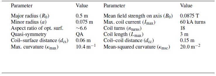


 L
 T
 L
 T
 B0
 (R,Z)
 ιk
 ϕ
 0
 π
 ϕ=0
 ϕ
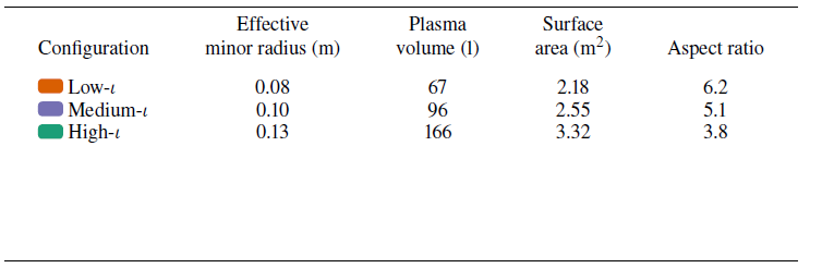

 20eV
 2.86keV

 ϕ

 0.1
 ϕ=0
 ι
 ι
 ι
 ϕ=0
 ϕ=180∘
 ϕ=0
 ϕ=180∘
 180∘
 0
 ϕ=0
 ϕ=180∘
 ι

 Q
 −2
 ϕ
 θ
 90∘

 LC
 ι
 ϕ=0.0∘,30.0∘,60.0∘,90.0∘
 LC
 0.1m
 40m
 10kWm−2

 z
 ϕ
 ϕ=90∘
 ϕ=0∘
 LC=36

 ϕ
 σ=1cm,ℓ=0.5

 σ=1cm,ℓ=0.5
 L
 T
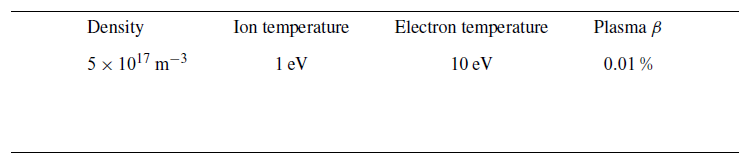

 ϕ=0
 ΔX-point=‖Γ~X-point(ϕ=0)−ΓX-point(ϕ=0)‖
 4cm
 ΔX
 maxt∈[0,1),i=1,…,6‖(Ξi(t)⋅ni(t))ni(t)+(Ξi(t)⋅bi(t))bi(t)‖
 ni(t),bi(t)
 ι

 Open access

